Improved Methods for Making Inferences About Multiple Skipped Correlations

ABSTRACT

A skipped correlation has the advantage of dealing with outliers in a manner that takes into account the overall structure of the data cloud. For p-variate data, $p\geq 2$, there is an extant method for testing the hypothesis of a zero correlation for each pair of variables that is designed to control the probability of one or more Type I errors. And there are methods for the related situation where the focus is on the association between a dependent variable and $p$ explanatory variables. However, there are limitations and several concerns with extant techniques. The paper describes alternative approaches that deal with these issues.

Keywords: Tests of independence, multivariate outliers, projection methods, Pearson’s correlation, Spearman’s rho

1 Introduction

For some unknown $p$-variate distribution, let $\tau_{jk}$ be some measure of association between variables $j$ and $k$, $1\leq j<k\leq p$. A basic goal is controlling the family wise error rate (FWE), meaning the probability of at least one Type I error, when testing

$$H_{0}:\tau_{jk}=0$$ (1)

for each $j<k$, where the alternative hypothesis is $H_{1}$: $\tau_{jk}\neq 0$.

Of course, one possibility is to take $\tau_{jk}$ to be Pearson’s correlation. It is well known, however, that Pearson’s correlation is not robust (e.g., Wilcox, 2017a). In particular, it has an unbounded influence function (Devlin et al., 1981). Roughly, this means that if one of the marginal distributions is altered slightly, the magnitude of $\rho$ can be changed substantially. A related concern is that the usual estimate of $\rho$, $r$, has a breakdown point of only $1/n$. This means, for example, that even a single outlier, properly placed, can completely dominate $r$.

Let $X_{1},\ldots,X_{p}$ denote $p$ random variables. As is evident, a goal related to methods design to test (1) is to test

$$H_{0}:X_{j}\,{\rm and}\,X_{k}\,{\rm are\,independent}$$ (2)

for each $j<k$, where the alternative hypothesis is that there is some type of dependence. Note that when a method is based on an estimate of $\tau_{jk}$, if it assumes homoscedasticity (the variance of $X_{j}$ does not depend on the value of $X_{k}$), it can detect dependence that would be missed by a method designed to test (1) that is insensitive to heteroscedasticity. Consider, for example, the classic Student’s t-test for testing (1) based on Pearson’s correlation, $\rho_{jk}$. Even when $\rho_{jk}=0$, if there is heteroscedasticity, the probability of rejecting increases as the sample size gets large (e.g., Wilcox, 2017b). The reason is that the test statistic, T, uses the wrong standard error. So if the goal is to detect dependence, T might be more effective than a method that is insensitive to heteroscedasticity. But if the goal is to compute a confidence interval for $\tau_{jk}$, methods that assume homoscedasticity can be highly unsatisfactory. The goal here is to consider both situations: testing (2) via some method based on an estimate of $\tau_{jk}$ as well as a method for testing (1) that allows heteroscedasticity.

Consider the usual linear regression model, where $X_{1},\ldots,X_{p}$ are $p$ predictors and $Y$ is some dependent variable of interest. Let $\tau_{yj}$ be some measure of association associated with $Y$ and $X_{j}$ ($j=1,\ldots,p$.) There is, of course, a goal related to (1), namely testing

$$H_{0}:\tau_{yj}=0$$ (3)

for each $j$ in a manner that controls FWE. Relevant results are included here.

Note that both (1) and (2) are not based on a linear model in the sense that no single variable is designated as the dependent variable with the remaining $p-1$ variables viewed as the explanatory variables. In the context of a linear model, an alternative to (3), with the goal of detecting dependence, is to test

$$H_{0}:\beta_{j}=0$$ (4)

for each $j$ ($j=1,\ldots,p$), using some robust regression estimator, where $\beta_{j}=0$ is the slope associated with the $j$th explanatory variable. From basic principles, the magnitude of the slopes can depend on which explanatory variables are included in the model. In particular, the magnitude of any slope can depend on the nature of the association between the corresponding explanatory variable and the other explanatory variables in the model. In contrast, the method used here to test (1) is not impacted in the same manner as will be made evident. So in terms of power, testing (1) can have more or less power than testing (4).

Now consider the situation where say $H_{0}$: $\beta_{1}=0$ is tested when the remaining explanatory variables are ignored. One could use some robust regression estimator to accomplish this goal. However, robust regression estimators can react differently to outliers, compared to the robust regression correlation used here. Details are described and illustrated in section 4.4 of this paper.

Numerous robust measures of association have been proposed that belong to one of two types (e.g., Wilcox, 2017a). The first, sometimes labeled Type M, are measures that guard against the deleterious impact of outliers among the marginal distributions. The two best-known Type M measures are Spearman’s rho and Kendall’s tau. A positive feature is that both have a bounded influence function (Croux & Dehon, 2010). Nevertheless, two outliers, properly placed, can have in inordinate impact on the estimate of these measures of association. In fact, imagine that boxplots are used to detect outliers among the first of two random variables, ignoring the second random variable, and none are found. Further imagine that no outliers among the second random variable are found, ignoring the first random variable. As illustrated in Wilcox (2017b, p. 239), it is still possible that there are outliers relative to the cloud of points that can have an inordinate impact on Spearman’s rho and Kendall’s tau. More generally, methods that deal only with outliers among each of the marginal distributions can be unsatisfactory.

Type O measures of association are designed to deal with the concern with Type M measures of association just described. A simple way to proceed is to use a skipped measure of association. That is, use a multivariate outlier detection method that takes into account the overall structure of the data cloud, remove any points flagged as outliers, and compute a measure of association (e.g., Pearson’s correlation) based on the remaining data. Skipped correlations are special cases of a general approach toward multivariate measures of location and scatter suggested by Stahel (1981) and Donoho (1982).

There are several outlier detection techniques that take into account the overall structure of a data cloud (e.g., Wilcox, 2017a, section 6.4). Consider a random sample of $n$ vectors from some multivariate distribution: $\mathbf{X}_{i}$ ($i=1,\ldots,n$). One general approach is to measure the distance of the point $\mathbf{X}_{i}$ from the center of the cloud of data with

$$D_{i}=\sqrt{({\bf X}_{i}-{\bf C})^{\prime}{\bf M}^{-1}({\bf X}_{i}-{\bf C})},$$

where $\mathbf{C}$ and $\mathbf{M}$ are robust measures of location and scatter, respectively, having reasonably high breakdown points. Among the many possible choices for $\mathbf{C}$ and $\mathbf{M}$ are the minimum volume ellipsoid estimator (Rousseeuw & van Zomeren, 1990), the minimum covariance determinant estimator (Rousseeuw & van Driessen,1999), the TBS estimator proposed by Rocke (1996). If $D_{i}$ is sufficiently large, $\mathbf{X}_{i}$ is flagged an outlier. There are several refinements of this approach, but the details go beyond the scope of this paper.

Here, following Wilcox (2003), a projection-type method is used, which is reviewed in section 2. The basic idea is that if a point is an outlier, then it should be an outlier for some projection of the $n$ points. This is not to suggest that it dominates all other methods. The only suggestion is that it is a reasonable choice with the understanding that there might be practical advantages to using some other technique. It will be evident that the approach used here is readily generalized to any measure of association that might be used in conjunction with any multivariate outlier detection technique that might be of interest.

Now, consider the strategy of removing points flagged as outliers using a projection method and then computing some measure of association based on the remaining data, say $\hat{\tau}_{jk}$. Wilcox (2003) describes a method for testing (1) when using Spearman’s rho. However, there are limitations and concerns that motivated this paper. First, a simple method for determining a 0.05 critical value for the test statistic, used by Wilcox, is available. In principle, simulations could be used to determine a critical value when testing at say the 0.01 level, but the efficacy of doing this is unknown. Second, when sampling form heavy-tailed distributions, the method avoids FWE greater than 0.055 in simulations reported by Wilcox (2003), but under normality the actual probability of one or more Type I errors can drop substantially below the nominal level. What would be desirable is a method that controls FWE in a manner that is less sensitive to changes in the distribution generating the data. Another issue that might be a concern is that the method is limited to using Spearman’s rho. It breaks down when using Pearson’s correlation instead. The goal here is to describe alternative approaches that deal with all of these limitations.

For $p=2$, Wilcox (2015) found that a percentile bootstrap method performed well in simulations, in terms of avoiding a Type I error probability greater than 0.05, when testing (1) at the 0.05 level, even when there is heteroscedasticity. So when $p>2$ a simple approach is to use this method in conjunction with some extant technique for controlling the probability of one or more Type I errors. However, as will be demonstrated, the actual level can be substantially smaller than the nominal level when the sample size is relatively small, which indicates that power can be relatively low. A method for dealing with this concern is derived.

The paper is organized as follows. Sections 2 and 3 review the approach used by Wilcox (2003). Section 2 describes the details of the outlier technique that was used and Section 3 reviews the method used to test (1). Section 4 describes the proposed methods. Section 5 reports simulation results and section 6 illustrates the methods using data from two studies. The first deals with the reading ability of children and the second deals with the processing speed in adults.

2 A Projection-Type Outlier Detection Method

The multivariate outlier detection technique used by Wilcox (2003) is computed as follows. Let $\hat{\xi}$ be some robust multivariate measure of location. Here, $\hat{\xi}$ is taken to be the marginal medians, but there is a collection of alternative estimators that might be used (e.g., Wilcox, 2017a, section 6.3). Let $\mathbf{X}_{1},\ldots,\mathbf{X}_{n}$ be a random sample from some multivariate distribution. Fix $i$ and for the point $\mathbf{X}_{i}$, project all $n$ points onto the line connecting $\hat{\xi}$ and $\mathbf{X}_{i}$ and let $D_{j}$ be the distance between the origin and the projection of $\mathbf{X}_{j}$. More formally, let

$$A_{i}=\mathbf{X}_{i}-\hat{\xi},$$

$$B_{j}=\mathbf{X}_{j}-\hat{\xi},$$

where both $A_{i}$ and $B_{j}$ are column vectors having length $p$, and let

$$C_{j}=\frac{A^{\prime}_{i}B_{j}}{B^{\prime}_{j}B_{j}}B_{j},$$

$j=1,\ldots,n$. Then when projecting the points onto the line between $X_{i}$ and $\hat{\xi}$, the distance of the $j$th projected point from the origin is

$$D_{j}=\|C_{j}\|,$$

where $\|C_{j}\|$ is the Euclidean norm of the vector $C_{j}$.

Next, a modification of the boxplot rule for detecting outliers is applied to the $D_{j}$ values, which has close similarities to one used by Carling (2000). Let $\ell=[n/4+5/12]$, where $[.]$ is the greatest integer function, let

$$h=\frac{n}{4}+\frac{5}{12}-\ell$$

and $k=n-\ell+1$. Let $D_{(1)}\leq\cdots\leq D_{(n)}$ be the $n$ distances written in ascending order. The so-called ideal fourths associated with the $D_{j}$ values are

$$q_{1}=(1-h)D_{(\ell)}+hD_{(\ell+1)}$$

and

$$q_{2}=(1-h)X_{(k)}+hX_{(k-1)}.$$

Then the jth point is declared an outlier if

$$D_{j}>M_{D}+\sqrt{\chi^{2}_{0.95,p}}(q_{2}-q_{1}),$$ (5)

where $M_{D}$ is the usual sample median based on the $D_{j}$ values and $\chi^{2}_{0.95,p}$ is the 0.95 quantile of a chi-squared distribution with $p$ degrees of freedom (cf. Rousseeuw and van Zomeren, 1999).

The process just described is for a single projection; for fixed $i$, points are projected onto the line connecting $\mathbf{X}_{i}$ to $\hat{\xi}$. Repeating this process for each $i$, $i=1,\ldots,n$, a point is declared an outlier if for any of these projections, it satisfies equation (4).

A simple and seemingly desirable modification of the method just described is to replace the interquartile range ($q_{2}-q_{1}$) with the median absolute deviation (MAD) measure of scale based on the $D_{j}$ values. So here, MAD is the median of the values

$$|D_{1}-M_{D}|,\ldots,|D_{n}-M_{D}|.$$

Then the jth point is declared an outlier if

$$D_{j}>M_{D}+\sqrt{\chi^{2}_{0.95,p}}\frac{{\rm MAD}}{0.6745},$$ (6)

where the constant 0.6745 is typically used because under normality, MAD/0.6745 estimates the standard deviation. One appealing feature of MAD is that it has a higher finite sample breakdown point versus the interquartile range. MAD has a finite sample breakdown point of approximately 0.5, while for the interquartile range it is only 0.25. Let $p_{n}$ be the outside rate per observation corresponding to some outlier detection method, which is the expected proportion of outliers based on a random sample of size $n$. A negative feature associated with (5) is that $p_{n}$ appears to be considerably less stable as a function of $n$. In the bivariate case, for example, it is approximately 0.09 with $n=10$ and drops below 0.02 as $n$ increases. For the same situations, $p_{n}$ based on equation (4) ranges between 0.043 and 0.038. Perhaps situations are encountered where the higher breakdown point associated with (5) is more important than having $p_{n}$ relatively stable as a function of the sample size $n$. But for present purposes, the approached based on (5) is not used.

3 A Review of an Extant Technique

Momentarily consider the bivariate case and let $r_{c}$ be skipped correlation when Pearson’s correlation is used after outliers are removed as described in section 2. An unsatisfactory approach to testing (1) is to simply use the test statistic

$$T=r_{c}\sqrt{\frac{m-2}{1-r^{2}_{c}}},$$

where $m$ is the number of observations left after outliers are discarded, and reject if $|T|$ exceeds the $1-\alpha/2$ quantile of Student’s T distribution with $m-2$ degrees of freedom. This approach is unsatisfactory, even under normality, roughly because the wrong standard error is being used. Wilcox (2003) illustrated that if this issue is ignored and this approach is used anyway, it results in poor control over the probability of a Type I error.

Returning to the general case $p\geq 2$, Wilcox (2003) proceeded as follows given the goal of controlling FWE. Let $\hat{\tau}_{cjk}$ be Spearman’s correlation between variables $j$ and $k$ after outliers are removed. Let

$$T_{jk}=\hat{\tau}_{cjk}\sqrt{\frac{n-2}{1-\hat{\tau}_{cjk}^{2}}},$$

and let

$$T_{{\rm max}}={\rm max}|T_{jk}|,$$ (7)

where the maximum is taken overall $j<k$. The initial strategy was to estimate, via simulations, the distribution of $T_{{\rm max}}$ under normality when all correlations are zero and $p<4$, determine the 0.95 quantile, say $q$, for $n=10$, 20, 30, 40, 60, 100 and 200, and then reject $H_{0}:\tau_{cjk}=0$ if $|T_{jk}|\geq q$. However, for $p\geq 4$, this approach was unsatisfactory when dealing with symmetric, heavy-tailed distributions, roughly meaning that outliers are relatively common. More precisely, the estimate of FWE exceeded 0.075. So instead, the critical value $q$ was determined via simulations where data are generated from a g-and-h distribution (described in the next section) with $(g,\,h)=(0,\,0.5)$, which is a symmetric and heavy-tailed distribution. This will be called method M henceforth. Using instead Pearson’s correlation, the method just described did not perform well in simulations. Moreover, there are at least three practical concerns with method M, which were reviewed in the introduction.

4 The Proposed Methods

This section describes a method for testing (2), based on a skipped correlation, which is sensitive to heteroscedasticity as well as the extent to which $\tau_{jk}$ differs from zero. This is followed by methods for testing (1) that is designed to control FWE even when there is heteroscedasticity. Results dealing with (3) are described as well.

4.1 A Homoscedastic Method for Testing (2)

An outline of the proposed method for testing (2) is as follows. Let $X_{ij}$ ($i=1,\dots,n$; $j=1,\ldots,p$) be a random sample of $n$ vectors from a $p$-variate distribution. The basic idea is to generate bootstrap samples from each marginal distribution in a manner for which there is no association. Next, compute $T_{{\rm max}}$ based on these bootstrap samples yielding say $T^{*}$. This process is repeated $B$ times, which can be used to estimate the $1-\alpha$ quantile of the distribution of $T_{{\rm max}}$ when the null hypothesis is true for all $j<k$.

To be more precise, let $X^{*}_{11},\ldots,X^{*}_{n1}$ be a bootstrap sample from the first column of the data matrix, which is obtained by randomly sampling with replacement $n$ values from $X_{11},\ldots,X_{n1}$. Next, take an independent bootstrap sample from the second column yielding $X^{*}_{12},\ldots,X^{*}_{n2}$ and continue in this manner for all $p$ columns. So information about the marginal distributions is maintained but the bootstrap samples are generated in a manner so that all correlations are zero. Next, compute $T^{*}$, the value of $T_{{\rm max}}$ based on these $p$ bootstrap samples and repeat this process $B$ times yielding $T^{*}_{1},\ldots,T^{*}_{B}$. Here, $B=500$ is used, which generally seems to suffice, in terms of controlling the probability of a Type I error, when dealing with related situations (Wilcox, 2017a).

Next, put the $T^{*}$ values in ascending order yielding $T^{*}_{(1)}\leq\cdots\leq T^{*}_{(B)}$. Let $c=(1-\alpha)B$, rounded to the nearest integer. Then an estimate of the $1-\alpha$ quantile of the null distribution of $T_{{\rm max}}$ is $T^{*}_{(c)}$. However, simulations indicated that the Harrell and Davis (1982) quantile estimator performs a bit better and so it is used henceforth. That is, the $q$th quantile is estimated with

$$\hat{\theta}_{q}=\sum W_{b}T^{*}_{(b)},$$

where

$$W_{b}=P\left(\frac{b-1}{B}\leq U\leq\frac{b}{B}\right),$$

and $U$ has a beta distribution with parameters $(B+1)q$ and $(B+1)(1-q)$. So if the goal is to have the probability of one or more Type I errors equal to $\alpha$, then for any $j<k$, reject (2) if $|T_{jk}|\geq\hat{\theta}_{1-\alpha}$.

Notice that an analog of a p-value can be computed. That is, one can determine the smallest $\alpha$ value for which one or more of the $(p^{2}-p)/2$ hypotheses is rejected. Here this is done by finding the value $q$ that minimizes $|\hat{\theta}_{q}-T_{{\rm max}}|$. When using Spearman’s rho after outliers are removed, this will be called method SS henceforth. Using Pearson’s correlation will be called method SP.

Note that methods SS and SP are based on a nonparametric estimate of the marginal distributions. However, the estimate of the $1-\alpha$ quantile of the null distribution of $T_{{\rm max}}$ is done for a situation where there is homoscedasticity. That is, based on how the bootstrap samples were generated, any information regarding how the variance of $X_{j}$ depends on the value of $X_{k}$ is lost. If there is in fact heteroscedasticity, meaning that the variance of $X_{j}$ depends on the value of $X_{k}$, and if the goal is to test (1), not (2), methods SS and SP can be unsatisfactory based on simulations reported in section 5. For example, when testing at the 0.05 level, the actual FWE can exceed 0.10.

4.2 A Heteroscedastic Method for Testing (1)

Results in Wilcox (2015) hint at how one might proceed when testing (1). Focusing on $p=2$, he found that when a skipped correlation based on Pearson’s correlation, a basic percentile bootstrap method performs reasonably well in terms of avoiding a Type I error probability greater than 0.05 when testing at the 0.05 level. So in contrast to methods SS and SP, a bootstrap sample is obtained by sampling with replacement $n$ rows from the $n$-by-$2$ matrix $X_{ij}$. Next, compute the skipped correlation based on this bootstrap sample and label the result $\hat{\tau}^{*}$. Repeat this process $B$ times yielding $\hat{\tau}^{*}_{1},\ldots,\hat{\tau}^{*}_{B}$. Put these $B$ values in ascending order yielding $\hat{\tau}^{*}_{(1)},\ldots,\hat{\tau}^{*}_{(B)}$. Let $\ell=\alpha B/2$, rounded to the nearest integer and $u=B-\ell$. Then the $1-\alpha$ confidence interval for $\tau_{jk}$ is taken to be

$$(\hat{\tau}^{*}_{(\ell+1)},\,\hat{\tau}^{*}_{(u)}).$$ (8)

Letting $Q$ denote the proportion of $\hat{\tau}^{*}_{b}$ ($b=1,\ldots,B$) values less than zero, a (generalized) p-value is given by 2min{$Q$, 1-$Q$}. (For general theoretical results related to this method, see Liu & Singh, 1997.) The striking feature of the method is that there is little variation in the estimated Type I error probability among the situations considered in the simulations. For $n=40$, the estimates ranged between 0.021 and 0.030. For $n=20$, estimates are less than 0.020.

The results just summarized suggest a simple modification for dealing with $p\geq 2$ and for $\alpha\neq 0.05$: use simulations to estimate a critical p-value, $p_{\alpha}$, such that FWE is equal to $\alpha$ under normality and homoscedasticity. To elaborate, for any $j<k$, let $p_{jk}$ be the percentile bootstrap p-value when testing (1). Then proceed as follows:

• Generate $n$ observations from a p-variate normal distribution for which the covariance matrix is equal to the identity matrix.

• For the data generated in step 1, compute the p-value for each of the $C=(p^{2}-p)/2$ hypotheses using a percentile bootstrap method. Let $V$ denote the minimum p-value among the $C$ p-values just computed.

• Repeat steps 1 and 2 $D$ times yielding the minimum p-values $V_{1},\ldots,V_{D}$.

• Let $\hat{p}_{\alpha}$ be an estimate of $\alpha$ quantile of the distribution of $V$. Here the Harrell and Davis estimator is used.

• Reject any hypothesis for which $p_{jk}\leq\hat{p}_{\alpha}$.

Here, $D=1000$, which was motivated in part by the execution time required to estimate $p_{\alpha}$. Using a four quad Mac Book Pro with 2.5 GHz processor, execution time is about 15 minutes when $n=20$ and $p=4$. (An R function was used that takes advantage of multicore processor via the R package parallel.) Increasing the sample size to $n=40$, execution time exceeds 36 minutes. This will be called method ECP henceforth.

Method H

Note that FWE could be controlled using the method derived by Hochberg (1988), which is applied as follows. Compute a p-value for each of the $C$ tests to be performed and label them $P_{1},\dots,P_{C}$. Next, put the p-values in descending order yielding $P_{[1]}\geq P_{[2]}\geq\cdots\geq P_{[C]}$. Proceed as follows:

• Set k = 1.

• If $P_{[k]}\leq d_{k}$, where $d_{k}=\alpha/k$, reject all $C$ hypotheses; otherwise, go to step 3.

• Increment $k$ by 1. If $P_{[k]}\leq d_{k}$, stop and reject all hypotheses having a p-value less than or equal to $d_{k}$.

• If $P_{[k]}>d_{k}$, repeat step 3.

This will be called method H henceforth.

Method H avoids the high execution time associated with estimating the critical p-value, $p_{\alpha}$, used by method ECP. But with a relatively small sample size, this approach will have relatively low power roughly because the actual FWE can be considerably less than the nominal level. This was expected because as previously noted, when $p=2$, the actual level can be considerably less than the nominal level. For example, with $p=4$ and $n=20$, FWE is approximately 0.007 under normality and homoscedasticity when the nominal level is 0.05. A modification of method H that deals with this issue, which also avoids the excessively high execution time due to estimating $p_{\alpha}$, is described in section 4.3. There are other methods for controlling FWE that are closely related to Hochberg’s method (e.g., Wilcox, 2017, section 12.1), but it is evident that again the actual level can be substantially smaller than the nominal level.

Method L

Observe that both methods H and ECP are readily extended to testing (3). Now a skipped correlation refers to the strategy of removing outliers based on $(Y_{i},\mathbf{X}_{i})$ ($i=1,\ldots,n$) and computing some measure of association using the remaining data. The modification of ECP, aimed at testing (3), is called method L henceforth. Another approach is, for each $j$, remove outliers among $(Y_{i},X_{ij})$, ignoring the other $p-1$ independent variables, and then compute a measure of association ($j=1,\ldots,p$). Perhaps there is some practical advantage to this latter approach, but it substantially increases execution time, so it is not pursued.

4.3 Improving Methods H and L: Methods L3 and H1

This section describes a modification of method H aimed at testing (1) and method L aimed at testing (3) that avoid the high execution time associated with method ECP. First consider testing (3) via method L in conjunction with Pearson’s correlation. Momentarily focus on the case of a single independent variable ($p=1$). Simulations indicate that $p_{\alpha}$ slowly decreases to $\alpha$ as $n$ increases. For $\alpha=0.05$ and $n=30$, $p_{\alpha}$ is estimated to 0.087. For $n=80$, 100 and 120 the estimates are 0.076, 0.062 and 0.049, respectively. So the basic idea is to use simulations to estimate the distribution of the p-value for a few selected sample sizes and use the results to get an adjusted p-value. The estimate is based on the approach used in conjunction with method ECP, only now $D=2000$ replications are used. Preliminary simulations suggest using estimates for $n=30$, 60, 80 and 100.

To elaborate (still focusing on $p=1$) let $V_{n}$ denote the vector of p-values corresponding to $n$ and stemming from the simulation just described. Let $p_{y1}$ be the bootstrap p-value when testing (3) via method L. Then given $V_{n}$, an adjusted p-value can be computed, which is simply the value $q$ such that $\hat{\theta}_{q}(V_{n})=p_{y1}$. For example, if the bootstrap p-value is 0.08, and $V_{n}$ indicates that the level of the test is 0.05 when $p_{\alpha}=0.08$ is used, then the adjusted p-value is 0.05. Here, adjusted p-values are computed in the following manner: use $V_{30}$ when $20\leq n\leq 40$, use $V_{60}$ when $41<n\leq 70$, use $V_{80}$ when $71<n\leq 100$ and $V_{100}$ when $101<n\leq 120$. For $n>120$, no adjustment is made.

Now consider $p>1$ and for each $j$ ($j=1,\ldots,p)$, let $\tilde{p}_{j}$ be the adjusted p-value when testing (3) via method L. The strategy is to use these adjusted p-values in conjunction with Hochberg’s method to control FWE. This will be called method L3. As is evident, the same strategy can be used when testing (1); this will be called method H1 henceforth.

4.4 Comments on Using a Robust Regression Estimator

Now consider the usual linear model involving a single explanatory variable and focus on the goal of testing $H_{0}$: $\beta_{1}=0$. There are several robust regression estimators that might be used that have a high breakdown point. They include the M-estimator derived by Coakley and Hettmansperger (1993), the MM-estimator derived by Yohai (1987), as well as the Theil (1950) and Sen (1964) estimator. The first two estimators have the highest possible breakdown point, 0.5. The breakdown point of the Theil–Sen estimator is approximately 0.29. Currently, a percentile bootstrap method appears to be a relatively good technique for testing $H_{0}$: $\beta_{1}=0$ when dealing with both non-normality and a heteroscedastic error term (Wilcox, 2017a). But despite the relatively high breakdown points, a few outliers among $(Y_{1},X_{1}),\ldots,(Y_{n},X_{n})$ can have an inordinate impact on the estimate of the slope as illustrated in Wilcox (2017a, section 10.14.1). Moreover, the impact of outliers on any of these robust regression estimator can differ substantially from the impact on the skipped correlation, which can translate into differences in power.

As an illustration, consider the situation where $Y=X+\epsilon$, where $\epsilon$ has a standard normal distribution, the sample size is $n=30$ and two outliers are introduced by setting $(X_{1},Y_{1})=(X_{2},Y_{2})=(2,1,-3.4)$. Power using methods L is 0.53 (based on a simulation with 2000 replications) compared to 0.33 using the MM-estimator. The reason is that the skipped correlation is better able to detect and eliminate the two outliers. But this is not to suggest that method L dominates in terms of power. When using the MM-estimator, outliers can inflate the estimate of the slope resulting in more power. The same issue arises using the other robust regression estimators previously listed—evidently no method dominates in terms of power. The only certainty is that the choice of method can make a practical difference.

5 Simulation Results

Simulations were used to check the small sample properties of method SS and SP for the exact same situations used by Wilcox (2003). Observations were generated where the marginal distributions are independent with each having one of four g-and-h distributions (Hoaglin, 1985), which contains the standard normal distribution as a special case. If $Z$ has a standard normal distribution, then

$$W=\left\{\begin{array}[]{ll}\frac{{\rm exp}(gZ)-1}{g}{\rm exp}(hZ^{2}/2),&\mbox{if $g>0$}\\ Z{\rm exp}(hZ^{2}/2),&\mbox{if $g=0.$}\end{array}\right.$$ (9)

has a g-and-h distribution where $g$ and $h$ are parameters that determine the first four moments. The four distributions used here were the standard normal ($g=h=0$), a symmetric heavy-tailed distribution ($h=0.5$, $g=0$), an asymmetric distribution with relatively light tails ($h=0$, $g=0.5$), and an asymmetric distribution with heavy tails ($g=h=0.5$).

Table 1 shows the theoretical skewness and kurtosis for each distribution considered. When $g>0$ and $h>1/k$, $E(W^{k})$ is not defined and the corresponding entry in Table 1 is left blank. Plots of the four distributions are shown in Figure 1. Additional properties of the g-and-h distribution are summarized by Hoaglin (1985).

Table 1: Some properties of the g-and-h distribution.

g	h	$\kappa_{1}$	$\kappa_{2}$
0.0	0.0	0.00	3.0
0.0	0.5	—	—
0.5	0.0	1.75	8.9
0.5	0.5	—	—

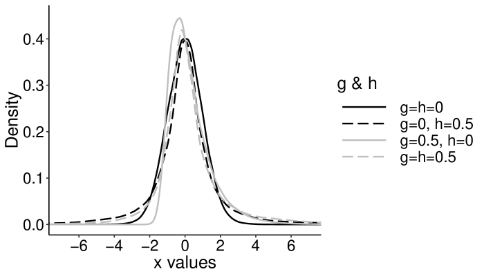
Figure 1: The four g-and-h distributions used in the simulations.

First consider methods SS and SP for testing (2). Each replication in the simulations consisted of generating $n$ observations and applying both methods SS and SP. The actual probability of one or more Type I errors was estimated with the proportion times there were one or more rejections among 5000 replications. Table 2 reports the estimated probability of one or more Type I errors when $n=20$, $p=4$ and 5, and $\alpha=0.05$, 0.025 and 0.01. The values in Table 2 for method M were taken from Wilcox (2003).

Table 2: Estimates of the actual FWE, $n=20$, using methods M, SP and SS

$p$	$g$	$h$	Method	$\alpha=0.05$	$\alpha=0.025$	$\alpha=0.01$
4	0.0	0.0	M	0.033	—-	—-
4	0.0	0.0	SP	0.058	0.023	0.011
4	0.0	0.0	SS	0.048	0.024	0.007
4	0.0	0.5	M	0.050	—-	—-
4	0.0	0.5	SP	0.060	0.031	0.013
4	0.0	0.5	SS	0.055	0.028	0.011
4	0.5	0.0	M	0.037	—-	—-
4	0.5	0.0	SP	0.064	0.031	0.013
4	0.5	0.0	SS	0.056	0.026	0.011
4	0.5	0.5	M	0.055	—-	—-
4	0.5	0.5	SP	0.050	0.026	0.010
4	0.5	0.0	SS	0.050	0.023	0.009
5	0.0	0.0	M	0.015	—-	—-
5	0.0	0.0	SP	0.065	0.030	0.014
5	0.0	0.0	SS	0.047	0.028	0.008
5	0.0	0.5	M	0.050	—-	—-
5	0.0	0.5	SP	0.049	0.024	0.008
5	0.0	0.5	SS	0.051	0.024	0.009
5	0.5	0.0	M	0.019	—-	—-
5	0.5	0.0	SP	0.069	0.034	0.013
5	0.5	0.0	SS	0.056	0.028	0.010
5	0.5	0.5	M	0.054	—-	—-
5	0.5	0.5	SP	0.042	0.020	0.008
5	0.5	0.0	SS	0.055	0.028	0.012
M=Wilcox’s method
SP=Pearson’s correlation
SS=Spearman’s correlation

Although the importance of a Type I error probability can depend on the situation, Bradley (1978) suggested that as a general guide, when testing at the $\alpha$ level, the actual level should be between $0.5\alpha$ and $1.5\alpha$. As can be seen, method SS always has estimates closer to the nominal level than method M when testing at the 0.05 level. Moreover, both SS and SP satisfy Bradley’s criterion with method SP a bit less satisfactory than method SS in terms of controlling FWE.

Note that when using method SP, the largest estimate in Table 2, when testing at the 0.05 level, occurs when $g=0.5$ and $h=0$. When $p=4$ the estimate is 0.064, and it is 0.069 when $p=5$. Increasing the sample size to $n=40$, the estimates were 0.054 and 0.062, respectively.

Table 3 reports results using method ECP that include situations where there is heteroscedasticty. The focus is on $p=2$ and $n=20$, so the results are relevant when testing (3) with method L. The number of replications was reduced to 2000 due to the high execution time. As a partial check on the impact of heteroscedasticty, data were generated where $X_{2}=\lambda(X_{1})\epsilon$, and $\epsilon$ has the same g-and-h distribution used to generate $X_{1}$. Three choices for $\lambda(X_{1})$ were used: $\lambda(X_{1})\equiv 1$ (homoscedasticity), $\lambda(X_{1})=|X_{1}|+1$, or $\lambda(X_{1})=1/(|X_{1}|+1)$. These three variance patterns are labeled VP 1, VP 2 and VP 3 henceforth. Estimates that do not satisfy Bradley’s criterion are in bold.

Table 3: Estimated Type I error probabilities using method ECP, $p=2$, $n=20$.

g	h	VP	Method	$\alpha=0.05$	$\alpha=0.025$	$\alpha=0.01$
0.0	0.0	1	HP	0.063	0.038	0.017
0.0	0.0	2	HP	0.061	0.032	0.017
0.0	0.0	3	HP	0.068	0.030	0.012
0.0	0.0	1	HS	0.051	0.023	0.014
0.0	0.0	2	HS	0.064	0.035	0.022
0.0	0.0	3	HS	0.055	0.032	0.016
0.0	0.5	1	HP	0.051	0.025	0.014
0.0	0.5	2	HP	0.049	0.024	0.014
0.0	0.5	3	HP	0.053	0.022	0.011
0.0	0.5	1	HS	0.050	0.035	0.019
0.0	0.5	2	HS	0.056	0.031	0.020
0.0	0.5	3	HS	0.053	0.030	0.021
0.5	0.0	1	HP	0.056	0.025	0.014
0.5	0.0	2	HP	0.061	0.029	0.016
0.5	0.0	3	HP	0.050	0.025	0.012
0.5	0.0	1	HS	0.051	0.032	0.022
0.5	0.0	2	HS	0.061	0.035	0.024
0.5	0.0	3	HS	0.047	0.027	0.016
0.5	0.5	1	HP	0.050	0.023	0.014
0.5	0.5	2	HP	0.048	0.023	0.011
0.5	0.5	3	HP	0.046	0.021	0.012
0.5	0.5	1	HS	0.047	0.029	0.016
0.5	0.5	2	HS	0.051	0.028	0.017
0.5	0.5	3	HS	0.050	0.028	0.017

Note that in Table 3, given $g$ and $h$, the estimates under homoscedasticity differ very little from the estimates when there is heteroscedasticity. All indications are that method ECP performs reasonably well when testing at the 0.05 or 0.025 level. However, with $n=20$, control over the Type I error probability might be viewed as being unsatisfactory in some situations when testing at the 0.01 level. But another issue is how well it performs, in terms of controlling FWE, when $p>2$. Table 4 reports results when $p=4$ and $n=20$. All of the estimates satisfy Bradley’s criterion.

Table 4: Estimates of FWE using method ECP, $p=4$, $n=20$

g	h	Method	$\alpha=0.05$	$\alpha=0.025$	$\alpha=0.01$
0.0	0.0	HP	0.051	0.025	0.011
0.0	0.0	HS	0.057	0.030	0.019
0.0	0.5	HP	0.043	0.024	0.008
0.0	0.5	HS	0.057	0.030	0.018
0.5	0.0	HP	0.043	0.021	0.011
0.5	0.0	HS	0.058	0.034	0.017
0.5	0.5	HP	0.050	0.019	0.008
0.5	0.5	HS	0.058	0.034	0.017

Of course, controlling FWE comes at the price of reducing power. Consider the situation where $p=5$ , $n=50$ and vectors of observations are sampled from a multivariate normal distribution having a common correlation of 0.3. If no adjustment aimed at controlling FWE is made, and $H_{0}$: $\tau_{12}=0$ is tested at the 0.05 level using HP, power was estimated to be 0.48. But if FWE is controlled, power is only 0.20.

Table 5 reports results for method L3 for $g=h=0$ (normality), $p=3(1)9$, and $n=30$ and 50. As can be seen, Bradley’s criterion is met for $p=3(1)8$ except for $p=7$ and $\alpha=0.05$, where the estimate is 0.078. For $p=9$, the method begins to breakdown. For $p=10$, not shown in Table 5, L3 performs well for $\alpha=0.05$, but the estimated level is substantially less than the nominal level for $\alpha=0.025$ and 0.01; the estimates are 0.014 and 0.000 respectively.

Table 5: Estimates of FWE using method L3, $g=h=0$

$p$	$n$	$\alpha=0.05$	$\alpha=0.025$	$\alpha=0.01$
3	30	0.057	0.031	0.010
3	50	0.065	0.040	0.015
4	30	0.057	0.028	0.018
4	50	0.056	0.024	0.005
5	30	0.060	0.035	0.012
5	50	0.064	0.025	0.009
6	30	0.066	0.033	0.013
6	50	0.062	0.020	0.010
7	30	0.063	0.038	0.015
7	50	0.078	0.022	0.013
8	30	0.065	0.031	0.018
8	50	0.060	0.020	0.011
9	30	0.077	0.041	0.026
9	50	0.061	0.024	0.023

As for method H1, the results are similar to those in Table 5 for $p=3$ and 4. For $p=5$, it performs well for $\alpha=0.05$ but the estimated level is unsatisfactory, based on Bradley’s criterion, for $\alpha=0.025$ and 0.01.

6 Two Illustrations

This section provides two illustrations. The first stems from Wilcox (2003) who used data dealing with reading abilities in children to illustrate method M. The variables were a measure of digit naming speed, a measure of letter naming speed, and a standardized test used to measure the ability to identify words. The sample size is $n=73$ after eliminating any row with missing values. The data are available in the file read_dat.txt at https://dornsife.usc.edu/labs/rwilcox/datasets/.

The estimates of Pearson’s correlation are 0.106, $-0.034$ and $-0.590$. Using the usual Student’s T test with Pearson’s correlation, with no attempt to control FWE or remove outliers, the p-values associated with $\rho_{12}$, $\rho_{13}$, $\rho_{23}$, are 0.37, 0.76 and $<0.001$, respectively, indicating a significant, negative association between a measure of letter naming speed and a standardized test used to measure the ability to identify words. Using method M with Pearson’s correlation, the test statistics were $|T_{12}|=8.13$, $|T_{13}|=3.18$, and $|T_{23}|=5.62$, with an estimated critical value of $q=2.9$. The skipped correlations are estimated to be 0.69, $-0.35$ and $-0.55$, respectively, all three of which are significant at the 0.01 level. As is evident, the first two correlations differ substantially from the situation where Pearson’s correlation is used with the outliers included.

As for Spearman’s rho, the estimates when outliers are included are 0.453, $-0.269$ and $-0.602$, all three of which are significant at the 0.028 level based on a percentile bootstrap method that allows heteroscedasticity (e.g., Wilcox, 2017a). Using method M instead, the corresponding estimates are 0.72, $-0.41$ and $-0.54$. Note that the first estimate differs substantially from the estimate of Spearman’s rho when the outliers are retained, which illustrates that outliers can have a substantial impact on Spearman’s rho. And there is a moderately large difference between the second two estimates. Again, using M, all three hypotheses given by (2) are significant when testing at the 0.01 level. Method SS (Spearman’s rho) also rejects all three when testing at the 0.05 level. Even when FWE is set equal to 0.0011, one association is still indicated.

Method M indicates that there are associations, but as previously explained, it can be unsatisfactory when the goal is to make inferences about the skipped correlation. Using instead method ECP, based on Pearson’s correlation, the three p-values are now $<$0.001, 0.028 and $<$0.001, respectively. The Hochberg adjusted p-values stemming from H1 are 0.002, 0.020 and 0.002. But for method ECP, the critical p-value was estimated to be 0.026. So the second hypothesis is not quite significant at the 0.05 level, illustrating that in some situations, Hochberg’s method might offer a power advantage. For the situation at hand, the critical p-value used by H1 is 0.0765. That is, it uses Hochberg’s method by testing at the 0.0765 level, which results in FWE approximately equal to 0.05. Note that the final step using Hochberg’s method would be to test at the $0.0765/3=0.0255$ level. That is, in this particular situation, Hochberg’s method will have as much or more power than method ECP. Put another way, method ECP corresponds to using the Bonferroni method at the $3\times 0.026=0.078$ level, which is approximately equal to the level used by H1, which is 0.0765. And it is well-known that Hochberg’s method has as much or more power than the Bonferroni method.

The second illustration stems from a study by Bieniek et al. (2016) who reported EEG data from a cross-sectional sample of 120 participants, aged 18-81, who categorized images of faces and textures. Based on these data, an integrative measure of visual processing speed was computed, using the approach described in Rousselet et al. (2010). A basic issue was understanding the association between the dependent variable (processing speed) and age. Two other independent variables are included here: years of education and visual acuity. Pearson’s correlation between processing speed and age, education and visual acuity was estimated to be 0.573, $-0.247$ and $-0.309$, respectively. The corresponding p-values were $<0.001$, 0.006 and 0.001. Using method L3 to control FWE, again all three independent variables have a significant association with the dependent variable. The Hochberg adjusted p-values ranged between 0.0021 and 0.0028. The skipped correlations were 0.621, $-0.280$ and $-0.407$. So all three skipped correlations indicate a stronger association versus Pearson’s correlation.

7 Concluding Remarks

As was demonstrated, methods SS and SP address the three concerns associated with method M. However, not all practical limitations have been eliminated. First, computational issues arise when using methods SS and SP with $n=10$. Using the projection-type outlier detection method based on a bootstrap sample can result in MAD or the interquartile range being zero. That is, a projection-type outlier detection method cannot be applied due to division by zero. Even with a large sample size, if there are many tied values, this issue might occur.

As for testing (3), all indications are that method L3 is reasonably satisfactory, in terms of controlling Type I error probabilities, when $p\leq 8$. For $p=9$ and 10, all indications that it continues to perform reasonably well when $\alpha=0.05$, but it can be unsatisfactory when testing at the 0.025 or 0.01 levels. As for testing (1), simulations indicate that method H1 is adequate when $p\leq 4$. Note that for $p=5$, ten hypotheses are being tested and that results related to method L3 suggest that it will not perform well when testing at the 0.025 and 0.01 levels. Simulation results confirm this. In contrast, methods SS and SP continue to perform reasonably well when $p=5$.

There are several other outlier detection methods that deserve serious consideration (e.g., Wilcox, 2017a). A few simulations were run where the projection-type outlier detection method was replaced by the method derived by Rousseeuw and van Zomeren (1990), as well as a method based in part on the minimum covariance determinant estimator (e.g., Wilcox, 2017a, section 6.3.2). Results were very similar to those presented here, but a more definitive study is needed.

Finally, the R function mscorpb applies SP by default, which is aimed at testing (2). Method SS can be applied by setting the argument corfun=spear. The function contains an option for using alternative outlier detection techniques. As for testing (1), the function mscorci applies method H by default in conjunction with Pearson’s correlation. Setting the argument hoch=FALSE, method ECP is used. Setting the argument corfun equal to spear, Spearman’s rho is used. To reduce execution time, method H1 can be used via the R function mscorciH. As for testing (3), the R function scorregci can be used. If the goal is merely to estimate the skipped correlations without testing hypotheses, use the R function scorreg. A Matlab implementation of the skipped correlation is also available (Pernet, et al., 2013.) The R function scorregciH applies method L3. All of these functions are being added to the R package WRS. For a more detailed description of how the data in section 6 were analyzed using these functions, see Wilcox et al. (2018).

References

Bieniek, M. M., Bennett, P. J., Sekuler, A. B. & Rousselet, G. A. (2016). A robust and representative lower bound on object processing speed in humans. European Journal of Neuroscience, 44, 1804–1814.

Bradley, J. V. (1978). Robustness? British Journal of Mathematical and Statistical Psychology, 31, 144–152.

Carling, K. (2000). Resistant outlier rules and the non-Gaussian case. Computational Statistics & Data Analysis, 33, 249–258.

Croux, C. & Dehon, C. (2010). Influence functions of the Spearman and Kendall Correlation measures. Statistical Methods and Applications, 19, 497–515.

Devlin, S. J., Gnanadesikan, R. & Kettenring, J. R. (1981). Robust estimation of dispersion matrices and principal components. Journal of the American Statistical Association, 76, 354–362.

Donoho, D. L. (1982). Breakdown properties of multivariate location estimators. PhD qualifying paper, Harvard University

Harrell, F. E. & Davis, C. E. (1982). A new distribution-free quantile estimator. Biometrika, 69, 635–640.

Hoaglin, D. C. (1985) Summarizing shape numerically: The g-and-h distributions. In D. Hoaglin, F. Mosteller & J. Tukey (Eds.) Exploring Data Tables, Trends and Shapes. New York: Wiley.

Hochberg, Y. (1988). A sharper Bonferroni procedure for multiple tests of significance. Biometrika, 75, 800–802.

Liu, R. G. & Singh, K. (1997). Notions of limiting P values based on data depth and bootstrap. Journal of the American Statistical Association, 92, 266–277.

Pernet, C. R., Wilcox, R. & Rousselet, G A. (2013). Robust correlation analyses: a Matlab toolbox for psychology research. Frontiers in Quantitative Psychology and Measurement. DOI=10.3389/fpsyg.2012.00606

Rousseeuw, P. J. & van Zomeren, B. C. (1990). Unmasking multivariate outliers and leverage points. Journal of the American Statistical Association, 85, 633–639.

Rousselet, G. A., Gaspar, C. M., Pernet, C. R., Husk, J. S., Bennett, P. J. & Sekuler, A. B. (2010). Healthy aging delays scalp EEG sensitivity to noise in a face discrimination task. Frontiers in psychology, 1.

Stahel, W. A. (1981). Breakdown of covariance estimators. Research report 31, Fachgruppe für Statistik, E.T.H Zurich.

Wilcox, R. R. (2003). Inferences based on multiple skipped correlations. Computational Statistics & Data Analysis, 44, 223–236.

Wilcox, R. R (2015). Inferences about the skipped correlation coefficient: Dealing with heteroscedasticity and non-normality. Journal of Modern and Applied Statistical Methods, 14, 2–8.

Wilcox, R. R. (2017a). Introduction to Robust Estimation and Hypothesis Testing, 4th Ed. San Diego, CA: Academic Press.

Wilcox, R. R. (2017b). Understanding and Applying Basic Statistical Methods Using R. New York: Wiley.

Wilcox, R., Pernet, C. & Rousselet, G. (2018). Improved methods for making inferences about multiple skipped correlations. figshare. https://doi.org/10.6084/m9.figshare.5768301.v1