Semi-Heuristic Parameter Choice Rules for Tikhonov Regularisation with Operator Perturbations

Abstract

We study the choice of the regularisation parameter for linear ill-posed problems in the presence of data noise and operator perturbations, for which a bound on the operator error is known but the data noise-level is unknown. We introduce a new family of semi-heuristic parameter choice rules that can be used in the stated scenario. We prove convergence of the new rules and provide numerical experiments that indicate an improvement compared to standard heuristic rules.

Keywords: regularisation, parameter choice rules, ill-posed problems, inverse problems, operator perturbations

1 Introduction

The framework of this study are linear ill-posed problems with noisy data and an operator perturbation. The basis is the following well-known abstract model equation

$$Ax=y,$$ (1)

with $A\in\mathcal{L}(X,Y)$, a continuous linear operator acting between two Hilbert spaces with non-closed range, which, for simplicity, is furthermore assumed to be injective. The contents of this paper remain valid for $A$ not injective, however. In the following we denote by $x^{\dagger}$ the minimum-norm least squares solution of (1).

We assume that both the data and the operator are perturbed, i.e.,

$${y_{\delta}}=y+e,\qquad\|e\|\leq\delta,$$

where $e$ denotes data error and $\delta$ the noise level. The model is further corrupted as a consequence of the operator error

$$A_{\eta}=A+\Delta A,\qquad\|\Delta A\|\leq\eta,$$

where $\Delta A$ is a bounded operator perturbation with magnitude bounded by $\eta$. We refer the reader to [15, 17, 14, 19] for further discussion regarding ill-posed problems with operator perturbations. There, one may find discussion of the generalised discrepancy principle which is an a-posteriori parameter choice rule requiring knowledge of both the data and operator noise levels.

The specific situation that we consider here, which is often met in practical situations, is that we suppose we have knowledge of the operator noise level, i.e., we assume $\eta$ known, but we do not know the level of the data error, $\delta$.

It is an obvious fact that such problems require regularisation, and for this study, we employ Tikhonov regularisation:

$${x_{\alpha,\delta,\eta}} =(A_{\eta}^{*}A_{\eta}+\alpha I)^{-1}A_{\eta}^{*}{y_{\delta}},$$ (2)

with a regularisation parameter $\alpha$ and only the mentioned bound on the perturbed operator available [18, 3]. For later reference, we furthermore define two auxiliary functions

$${x_{\alpha,\delta}} =(A^{*}A+\alpha I)^{-1}A^{*}{y_{\delta}},$$

$$x_{\alpha} =(A^{*}A+\alpha I)^{-1}A^{*}y.$$

The choice of the regularisation parameter (here $\alpha$) is an important and delicate issue for any regularisation method. The overall aim is to obtain convergence of the computed solution ${x_{\alpha,\delta,\eta}}$ to the exact solution when all error terms $\delta,\eta$ vanish:

$$\|{x_{\alpha,\delta,\eta}}-x^{\dagger}\|\to 0\qquad\text{ as }\delta\to 0,\eta\to 0.$$ (3)

To this end, one must select a rule for choosing the appropriate parameter $\alpha$. If $\delta$ was known, there are parameter choice rules that provide such a convergence and even rates of convergence.

However, when $\delta$ is unknown, as assumed in this paper, the choice of $\alpha$ is less standard and has to be done by heuristic rules, i.e., $\alpha$ is selected only depending on the given noisy data ${y_{\delta}}$ without explicit reference to $\delta$. The best-understood methods in this class are the minimisation-based ones, on which we build our methods as well.

The novelty of this paper is the use and analyis of semi-heuristic parameter choice rules, where an assumed known operator bound, $\eta$, is combined with the $\delta$-free heuristic rules. This paper is organised as follows: in Section 2, we introduce and motivate the use of semi-heuristic rules, and we provide a convergence analysis. In Section 3, we illustrate the theory by numerical results. Additionally, whilst the reader may be referred to [13] for the performance of the quasioptimality rule in the presence of a noisy operator, the performance of other heuristic rules in this setting has yet to be investigated. We subsequently shed new light on this as a byproduct of our comparison with the semi-heuristic rules.

2 Semi-heuristic parameter choice rules

As explained in the introduction, heuristic rules are employed in the case of unknown noise level $\delta$ (without operator perturbations).

Minimisation-based heuristic rules entail minimising a functional $\psi(\alpha,A,{y_{\delta}})$ with

$$\psi:[0,\alpha_{\text{max}}]\times\mathcal{L}(X,Y)\times Y\to\mathbb{R}\cup\{\infty\}.$$

The regularisation parameter is then selected as

$${\alpha_{*}}=\operatorname*{argmin}_{\alpha\in[0,\alpha_{\text{max}}]}\psi(\alpha,A,y_{\delta}),$$ (4)

which obviously does not depend on $\delta$.

Our methods use the following classical examples of $\psi$-functionals (see, e.g., [9]):

• The heuristic discrepancy functional

  $$\psi_{HD}(\alpha,A,y_{\delta}):=\frac{\|Ax_{\alpha,\delta,\eta}-y_{\delta}\|}{\sqrt{\alpha}}.$$ (5)

• The Hanke-Raus functional

  $$\psi_{HR}(\alpha,A,y_{\delta}):=\|(AA^{\ast}+\alpha I)^{-1/2}(Ax_{\alpha,\delta}-y_{\delta})\|.$$ (6)

• The quasioptimality functional

  $$\psi_{QO}(\alpha,A,y_{\delta}):=\left\|\alpha\frac{d}{d\alpha}x_{\alpha,\delta}\right\|.$$ (7)

In the linear case (as in the present setting), we can write these in terms of filter functions $\Psi$:

$$\psi(\alpha,A,{y_{\delta}})=\|\Psi(\alpha,A){y_{\delta}}\|.$$

In particular, the following filter functions

$$\Psi_{HD}(\alpha,A) :=\sqrt{\alpha}(AA^{*}+\alpha I)^{-1},$$

$$\Psi_{HR}(\alpha,A) :=\alpha(AA^{*}+\alpha I)^{-3/2},$$

$$\Psi_{QO}(\alpha,A) :=\alpha(A^{*}A+\alpha I)^{-2}A^{*}$$

may be associated with the heuristic discrepancy, Hanke-Raus and quasioptimality rules, respectively [7, 4].

Meanwhile, a convergence theory for such heuristic parameter choice rules has also been established. A central ingredient is that a noise condition has to be postulated in order for these methods to work. Such a condition, which links the operator, the data error and the solution, provides a deep understanding when such methods are successful. Essentially, a noise condition is satisfied if the data noise is sufficiently irregular. More precisely, we assume that for the specific choice of $\psi$, there exists a constant $C_{nc}$ such that for all given noisy data ${y_{\delta}}$ and exact data $y$, the following inequality is satisfied

$$\|{x_{\alpha,\delta}}-x_{\alpha}\|\leq C_{nc}\|\Psi(\alpha,A)({y_{\delta}}-y)\|\qquad\forall\alpha\in[0,\alpha_{\text{max}}],$$

or, equivalently,

$$\|(A^{*}A+\alpha I)^{-1}A^{*}({y_{\delta}}-y)\|\leq C_{nc}\psi(\alpha,A,{y_{\delta}}-y)\qquad\forall\alpha\in[0,\alpha_{\text{max}}].$$ (8)

See [9, 10] for a more detailed discussion which gives more explicit representations and justification for the noise conditions using spectral theory.

Such inequalities are satisfied for the above mentioned classical $\psi$-functionals for many realistic instances of “data noise”, e.g., for white or coloured noise [10, 11].

The fact that prohibits the direct use of a minimisation-based rule with, say, a functional of the form $\psi(\alpha,A_{\eta},y_{\delta}),$ in our case, is that we are faced with an additional operator error, which is usually not random or irregular and hence it would be unrealistic to assume that for the operator perturbation an analogous inequality holds. The remedy is to employ a modified functional, which uses the noisy operator $A_{\eta}$, but is designed to emulate a functional for the unperturbed operator. Therefore, we propose to subtract from the classical $\psi$-functional a term which should behave approximately like $\psi(\alpha,A,y_{\delta})-\psi(\alpha,A_{\eta},y_{\delta}).$

Thus, the semi-heuristic rule is of the following type: firstly, the regularisation parameter $\alpha={\alpha_{*}}$ is chosen similarly to (4) by a minimisation of

$$\bar{\psi}(\alpha,A_{\eta},{y_{\delta}}):=\psi(\alpha,A_{\eta},{y_{\delta}})-R(\alpha,A_{\eta},{y_{\delta}},\eta)$$ (9)

with $\psi$ being one of the classical heuristic functionals above, (5)–(7), and a functional $R$ (to be specified below) that compensates the operator error. Secondly, to guarantee a minimiser and convergence of the regularized solution, we restrict the minimisation to an interval $[\gamma,\alpha_{max}]$, where the lower bound $\gamma$ is selected depending on $\eta$ (but not on $\delta$):

$$\alpha_{*}:=\alpha(\eta,{y_{\delta}}):=\operatorname*{argmin}_{\alpha\in[\gamma,\alpha_{\text{max}}]}\bar{\psi}(\alpha,A_{\eta},{y_{\delta}}),\qquad\gamma=\gamma(\eta)>0.$$ (10)

In this way, we combine heuristic rules with an $\eta$-based choice.

We propose and investigate two classes of compensating functionals $R$ labelled as (SH1) and (SH2).

$$\bar{\psi}(\alpha,A_{\eta},{y_{\delta}})=\psi(\alpha,A_{\eta},y_{\delta})-D\eta\|{x_{\alpha,\delta,\eta}}\|,$$ (SH1) (11)

$$\bar{\psi}(\alpha,A_{\eta},{y_{\delta}})=\psi(\alpha,A_{\eta},y_{\delta})-D\frac{\eta}{\sqrt{\alpha}}.$$ (SH2) (12)

The constant $D$ should be chosen to obtain a scaling invariant functional. For instance, in the case of (SH1), we may choose $D\sim 1/\|A\|$ and for (SH2), as $D\sim\|y\|/\|A\|$. Note that the error estimate we derive is sharpest with the choice (11), although the numerical results are comparable.

The main goal of our analysis is to show convergence (3) for such semi-heuristic parameter choice rules.

2.1 Error estimates with operator noise

In the following, we assume the presence of operator noise. The following auxiliary result will be utilised extensively.

Lemma 1.

Let $\alpha\in[0,\alpha_{\text{max}}]$ and for $p\in\{0,\frac{1}{2},1\}$, define

$$B_{\eta,p}:=\begin{cases}(A^{\ast}_{\eta}A_{\eta})^{p}&\text{if }p\in\{0,1\},\\ A^{\ast}_{\eta}&\text{if }p=\frac{1}{2},\end{cases}\qquad B_{p}:=\begin{cases}(A^{\ast}A)^{p}&\text{if }p\in\{0,1\},\\ A^{\ast}&\text{if }p=\frac{1}{2}.\end{cases}$$

Let $\hat{B}_{\eta,p}$ and $\hat{B}_{p}$ be the operators we get from $B_{\eta,p}$ and $B_{p}$ by changing the roles of the operators $A_{\eta}\leftrightarrow A^{\ast}_{\eta}$ and $A\leftrightarrow A^{\ast}$, respectively. Then for $p\in\{0,\frac{1}{2},1\}$ and $q\in\{-1,-\frac{3}{2},-2\}$, there exist positive constants $C_{p,q}$ such that

$$\left\|(A^{\ast}_{\eta}A_{\eta}+\alpha I)^{q}B_{\eta,p}-(A^{\ast}A+\alpha I)^{q}B_{p}\right\|\leq C_{p,q}\frac{\eta}{\alpha^{\frac{1}{2}-p-q}}.$$ (13)

$$\left\|(A_{\eta}A^{\ast}_{\eta}+\alpha I)^{q}\hat{B}_{\eta,p}-(AA^{\ast}+\alpha I)^{q}\hat{B}_{p}\right\|\leq C_{p,q}\frac{\eta}{\alpha^{\frac{1}{2}-p-q}}.$$ (14)

Proof.

We prove (13), this gives (14) changing the roles of the operators $A_{\eta}\leftrightarrow A^{\ast}_{\eta}$ and $A\leftrightarrow A^{\ast}$. We recall the elementary estimates

$$\|(A^{\ast}A+\alpha I)^{-1}\|\leq\frac{1}{\alpha},\quad\|(A^{\ast}A+\alpha I)^{-1}A^{\ast}\|\leq\frac{1}{2\sqrt{\alpha}},\quad\|(A^{\ast}A+\alpha I)^{-1}A^{\ast}A\|\leq 1,$$ (15)

which also hold with $A$ and $A^{\ast}$ replaced by $A_{\eta}$ and $A_{\eta}^{\ast}$, respectively. For $p\in\{0,1\}$, it follows from some algebraic manipulations, the fact that $B_{p},B_{\eta.p}$ commute with the inverses below, and the previous estimates that

$$(A_{\eta}^{\ast}A_{\eta}+\alpha I)^{-1}B_{\eta,p}-B_{p}(A^{\ast}A+\alpha I)^{-1}$$

$$=(A_{\eta}^{\ast}A_{\eta}+\alpha I)^{-1}\left[B_{\eta,p}(A^{\ast}A+\alpha I)-(A_{\eta}^{\ast}A_{\eta}+\alpha I)B_{p}\right](A^{\ast}A+\alpha I)^{-1}$$

$$=(A_{\eta}^{\ast}A_{\eta}+\alpha I)^{-1}\left[B_{\eta,p}A^{\ast}A-A_{\eta}^{\ast}A_{\eta}B_{p}\right](A^{\ast}A+\alpha I)^{-1}$$

$$\qquad+\alpha(A_{\eta}^{\ast}A_{\eta}+\alpha I)^{-1}\left[B_{\eta,p}-B_{p}\right](A^{\ast}A+\alpha I)^{-1}.$$

In the case $p=0$ and $B_{\eta,0}=B_{0}=I$, we find

$$B_{\eta,0}A^{\ast}A-A_{\eta}^{\ast}A_{\eta}B_{0}=(A^{\ast}-A_{\eta}^{\ast})A+A_{\eta}^{\ast}(A-A_{\eta}),$$

which, using (15), gives $C_{0,-1}=1$. Similarly, we can prove that $C_{1,-1}=1$. For the case $p=\frac{1}{2}$, if $B_{\eta,p}=A_{\eta}^{\ast}$ and $B_{p}=A^{\ast}$, we obtain $C_{\frac{1}{2},-1}=\frac{5}{4}$ with minor modifications noting that $(A^{\ast}A+\alpha I)^{-1}A^{\ast}=A^{\ast}(AA^{\ast}+\alpha I)^{-1}$. The other cases of $q$ follow in a similar manner by

$$(A_{\eta}^{\ast}A_{\eta}+\alpha I)^{q}B_{\eta,p}-B_{p}(A^{\ast}A+\alpha I)^{q}$$

$$=(A_{\eta}^{\ast}A_{\eta}+\alpha I)^{q+1}\left[(A_{\eta}^{\ast}A_{\eta}+\alpha I)^{-1}B_{\eta,p}-B_{p}(A^{\ast}A+\alpha I)^{-1}\right]$$

$$+\left[(A_{\eta}^{\ast}A_{\eta}+\alpha I)^{q+1}-(A^{\ast}A+\alpha I)^{q+1}\right]B_{p}(A^{\ast}A+\alpha I)^{-1},$$

and by using (15) and the result for $q=-1$. For $q=-\frac{3}{2}$, we employ an additional identity from semigroup operator calculus [12],

$$(A_{\eta}^{\ast}A_{\eta}+\alpha I)^{-\frac{1}{2}}-(A^{\ast}A+\alpha I)^{-\frac{1}{2}}$$

$$\quad=\frac{\sin(\frac{\pi}{2})}{\pi}\int_{0}^{\infty}t^{-\frac{1}{2}}\left[(A_{\eta}^{\ast}A_{\eta}+(\alpha+t)I)^{-1}-(A^{\ast}A+(\alpha+t)I)^{-1}\right]\,\mathrm{d}t,$$

which leads to

$$\|(A_{\eta}^{\ast}A_{\eta}+\alpha I)^{-\frac{1}{2}}-(A^{\ast}A+\alpha I)^{-\frac{1}{2}}\| \leq\frac{C_{0,-1}\eta}{\pi}\int_{0}^{\infty}\frac{1}{\sqrt{t}(\alpha+t)^{\frac{3}{2}}}\,\mathrm{d}t$$

$$\leq\frac{2C_{0,-1}}{\pi}\frac{\eta}{\alpha},$$

thereby finishing the proof. ∎

As a consequence of the above lemma, we obtain some useful bounds.

Lemma 2.

For any of the parameter choice functionals $\psi\in\{\psi_{HD},\psi_{HR},\psi_{QO}\}$ (see (5)–(7)), any $\alpha\in[0,\alpha_{\text{max}}]$ we have

$$\psi(\alpha,A_{\eta},A_{\eta}x^{\dagger})\leq C_{p,q}\frac{\eta\|x^{\dagger}\|}{\sqrt{\alpha}}+\psi(\alpha,A,Ax^{\dagger}),$$ (16)

$$\psi(\alpha,A_{\eta},y_{\delta})\leq\frac{\delta}{\sqrt{\alpha}}+(1+C_{p,q})\frac{\eta\|x^{\dagger}\|}{\sqrt{\alpha}}+\psi(\alpha,A,Ax^{\dagger}),$$ (17)

with the constants $C_{p,q}$ from Lemma 1: $p=\frac{1}{2},$ $q=-1$ for the heuristic discrepancy, $p=\frac{1}{2},$ $q=-\frac{3}{2}$ for the Hanke-Raus, and $p=1,$ $q=-2$ for the quasioptimality functionals, respectively.

Proof.

The inequality (16) follows from (13) and (14), the inequality (17) from (16) and from the inequalities

$$\psi(\alpha,A_{\eta},y_{\delta}) \leq\psi(\alpha,A_{\eta},y_{\delta}-y)+\psi(\alpha,A_{\eta},(A-A_{\eta})x^{\dagger})+\psi(\alpha,A_{\eta},A_{\eta}x^{\dagger})$$

$$\leq\frac{\delta}{\sqrt{\alpha}}+\frac{\eta\|x^{\dagger}\|}{\sqrt{\alpha}}+\psi(\alpha,A_{\eta},A_{\eta}x^{\dagger}).$$

∎

We remark that the term $\psi(\alpha,A,Ax^{\dagger})$ converges to $0$ as $\alpha\to 0$; see, e.g., [10]. Furthermore, if $x^{\dagger}$ additionally satisfies a source condition [3], then the expression can be bounded by a convergence rate of order $\alpha$ (with some exponent depending on the source condition) that agrees with the standard rate for the approximation error $\|x_{\alpha}-x^{\dagger}\|$.

2.2 Convergence

Suppose that $\alpha_{*}$ is the selected parameter by the proposed parameter choice rules with the operator noise (10). In the following lemma, we show that for such a choice of parameter, it follows that ${\alpha_{*}}\to 0$ if all noise (with respect to both the data and the operator) vanishes:

Lemma 3.

Let $\alpha_{\ast}$ be selected as above, i.e., (10), with $\bar{\psi}$ as in (11) or (12) and $\psi\in\{\psi_{HD},\psi_{HR},\psi_{QO}\}$. Suppose there exist positive constants (not necessarily equal which we denote universally by $C$) such that $\|y_{\delta}\|\geq C$ for $\psi\in\{\psi_{HD},\psi_{HR}\}$ and $\|A_{\eta}^{\ast}y_{\delta}\|\geq C$ for $\psi=\psi_{QO}$.

If $\gamma=\gamma(\eta)$ is chosen such that $\frac{\eta}{\sqrt{\gamma}}\to 0$ as $\eta\to 0$ then

$$\alpha_{\ast}\to 0$$

as $\delta,\eta\to 0$.

Proof.

At first, we show some lower bounds for the parameter choice functionals. If $\|{y_{\delta}}\|\geq c_{0}$ and $\|A_{\eta}^{\ast}{y_{\delta}}\|\geq c_{0}$ then there exist constants such that

$$\psi(\alpha,A_{\eta},{y_{\delta}})\geq\begin{cases}C\sqrt{\alpha}&\text{ if }\psi=\psi_{HD},\\ C\alpha&\text{ if }\psi\in\{\psi_{HR},\psi_{QO}\}.\end{cases}$$ (18)

To see this, we get from the relation (here $s\geq 0$ arbitrary)

$$\|{y_{\delta}}\|=\|(A_{\eta}A_{\eta}^{\ast}+\alpha I)^{s}(A_{\eta}A_{\eta}^{\ast}+\alpha I)^{-s}{y_{\delta}}\|\leq\|(A_{\eta}A_{\eta}^{\ast}+\alpha I)^{s}\|\|(A_{\eta}A_{\eta}^{\ast}+\alpha I)^{-s}{y_{\delta}}\|$$

the inequality

$$\|(A_{\eta}A_{\eta}^{\ast}+\alpha I)^{-s}{y_{\delta}}\|\geq\frac{\|{y_{\delta}}\|}{\|(A_{\eta}A_{\eta}^{\ast}+\alpha I)^{s}\|}\geq\frac{c_{0}}{c_{1}^{s}},$$

with $c_{1}\geq\|A_{\eta}A_{\eta}^{\ast}+\alpha I\|$. This gives (18) for $\psi_{HD}$ ($s=1$) and $\psi_{HR}$ ($s=\frac{3}{2}$). The estimate (18) for $\psi_{QO}$ follows analogously:

$$\psi_{QO}=\alpha\|(A_{\eta}^{\ast}A_{\eta}+\alpha I)^{-2}A_{\eta}^{\ast}{y_{\delta}}\|\geq\alpha\frac{\|A_{\eta}^{\ast}{y_{\delta}}\|}{\|(\|A_{\eta}^{\ast}A_{\eta}+\alpha I)^{2}\|}\geq\alpha\frac{c_{0}}{c_{1}^{2}}.$$

By the standard error estimate

$$\|{x_{\alpha_{*},\delta,\eta}}\|\leq\frac{\|{y_{\delta}}\|}{\sqrt{\alpha_{\ast}}},$$

we find, for the case in which the compensating functional is chosen as in (11) using (18) and (17) with $t\in\{1/2,1\}$ suited to $\psi$ according to (18),

$$C{\alpha_{*}}^{t}-D\eta\frac{\|{y_{\delta}}\|}{\sqrt{{\alpha_{*}}}}\leq\bar{\psi}({\alpha_{*}},A_{\eta},y_{\delta})=\inf_{\alpha\in[\gamma,\alpha_{\text{max}}]}\bar{\psi}(\alpha,A_{\eta},y_{\delta})$$

$$\leq\inf_{\alpha\in[\gamma,\alpha_{\text{max}}]}\psi(\alpha,A_{\eta},y_{\delta})\leq\inf_{\alpha\in[\gamma,\alpha_{\text{max}}]}\left\{\frac{\delta}{\sqrt{\alpha}}+(1+C_{p,q})\frac{\eta\|x^{\dagger}\|}{\sqrt{\alpha}}+\psi(\alpha,A,Ax^{\dagger})\right\}$$

$$\leq\inf_{\alpha\in[\gamma,\alpha_{\text{max}}]}\left\{\frac{\delta}{\sqrt{\alpha}}++\psi(\alpha,A,Ax^{\dagger})\right\}+(1+C_{p,q})\frac{\eta\|x^{\dagger}\|}{\sqrt{\gamma}}.$$ (19)

Hence,

$$C{\alpha_{*}}^{t}\leq\inf_{\alpha\in[\gamma,\alpha_{\text{max}}]}\left\{\frac{\delta}{\sqrt{\alpha}}+\psi(\alpha,A,Ax^{\dagger})\right\}+(C+D)\frac{\eta}{\sqrt{\gamma}}\,.$$

It is not difficult to verify the same estimate analogously for the case in which the compensating functional is chosen according to (12).

Inserting the (nonoptimal) choice $\alpha=\delta+\gamma$ in the infimum, we obtain an upper bound that tends to $0$ as $\delta,\gamma\to 0$. By the hypothesis, the last two terms vanish, thereby proving the desired result. ∎

Remark.

If $\alpha_{\ast}$ is the minimizer of $\psi(\alpha,A_{\eta},y_{\delta})$, then this functional is the same as (11) and/or (12) with $D=0$ and one obtains the same result as above; namely, that $\alpha_{\ast}\to 0$ as $\delta,\eta\to 0$ provided that the conditions in the lemma are fulfilled.

Now, we can establish an estimate from above for the total error which is derived courtesy of a lower estimate of the parameter choice functional with the data error. Note that, due to Bakushinskii’s veto, this estimate cannot be derived without restricting the set of permissible noise [1], e.g., by a noise condition. At first we study bounds for the functional in (10).

Proposition 1.

Let ${\alpha_{*}}$ be selected according to (10) with $\bar{\psi}$ as in (11). Suppose that for the noisy data ${y_{\delta}}$, the noise condition (8) is satisfied. Then, for $\eta$ sufficiently small, we get the following error estimate for all $\psi\in\{\psi_{HD},\psi_{HR},\psi_{QO}\}$:

$$\|{x_{\alpha_{*},\delta,\eta}}-x^{\dagger}\|$$ (20)

$$\leq(1-D\eta C_{nc})^{-1}\bigg{[}C\frac{\eta\delta}{\alpha_{\ast}}+C_{nc}\inf_{\alpha\in[\gamma,\alpha_{\text{max}}]}\bar{\psi}(\alpha,A_{\eta},y_{\delta})+DC_{nc}\eta\|x^{\dagger}\|$$

$$\qquad\qquad+C\frac{\eta}{\sqrt{\alpha_{\ast}}}\|x^{\dagger}\|+C\psi(\alpha_{\ast},A,Ax^{\dagger})+{\alpha_{*}}\|(A^{*}A+{\alpha_{*}}I)^{-1}x^{\dagger}\|\bigg{]}.$$

Proof.

We begin by estimating the terms:

$$\|{x_{\alpha_{*},\delta,\eta}}-x^{\dagger}\|=\|(A_{\eta}^{*}A_{\eta}+{\alpha_{*}}I)^{-1}A_{\eta}^{*}{y_{\delta}}-(A_{\eta}^{*}A_{\eta}+{\alpha_{*}}I)^{-1}(A_{\eta}^{*}A_{\eta}+{\alpha_{*}}I)x^{\dagger}\|$$

$$\leq\|(A_{\eta}^{*}A_{\eta}+{\alpha_{*}}I)^{-1}\left[A_{\eta}^{*}{y_{\delta}}-A_{\eta}^{*}A_{\eta}x^{\dagger}-{\alpha_{*}}x^{\dagger}\right]\|$$

$$\leq\|(A_{\eta}^{*}A_{\eta}+{\alpha_{*}}I)^{-1}\left[A_{\eta}^{*}({y_{\delta}}-y)+A_{\eta}^{*}(A-A_{\eta})x^{\dagger}\right]\|+{\alpha_{*}}\|(A_{\eta}^{*}A_{\eta}+{\alpha_{*}}I)^{-1}x^{\dagger}\|$$

$$\leq\|(A_{\eta}^{*}A_{\eta}+{\alpha_{*}}I)^{-1}A_{\eta}^{*}({y_{\delta}}-y)\|+\frac{\eta}{2\sqrt{{\alpha_{*}}}}\|x^{\dagger}\|+{\alpha_{*}}\|(A_{\eta}^{*}A_{\eta}+{\alpha_{*}}I)^{-1}x^{\dagger}\|.$$

By (13), the last term can be bounded by

$${\alpha_{*}}\|(A_{\eta}^{*}A_{\eta}+{\alpha_{*}}I)^{-1}x^{\dagger}\| \leq{\alpha_{*}}\|\left[(A_{\eta}^{*}A_{\eta}+{\alpha_{*}}I)^{-1}-(A^{*}A+{\alpha_{*}}I)^{-1}\right]x^{\dagger}\|$$

$$\qquad\qquad\qquad\qquad+{\alpha_{*}}\|(A^{*}A+{\alpha_{*}}I)^{-1}x^{\dagger}\|$$

$$\leq C_{0,-1}\frac{\eta\|x^{\dagger}\|}{\sqrt{\alpha_{\ast}}}+{\alpha_{*}}\|(A^{*}A+{\alpha_{*}}I)^{-1}x^{\dagger}\|.$$

This leaves the remaining term:

$$\|(A_{\eta}^{*}A_{\eta}+{\alpha_{*}}I)^{-1}A_{\eta}^{*}({y_{\delta}}-y)\|$$

$$\leq\|\left[(A_{\eta}^{*}A_{\eta}+{\alpha_{*}}I)^{-1}A_{\eta}^{*}-(A^{*}A+{\alpha_{*}}I)^{-1}A^{*}\right]({y_{\delta}}-y)\|$$

$$\qquad\qquad\qquad+\|(A^{*}A+{\alpha_{*}}I)^{-1}A^{*}({y_{\delta}}-y)\|$$

$$\leq\frac{5\eta\delta}{4{\alpha_{*}}}+C_{nc}\psi({\alpha_{*}},A,{y_{\delta}}-y).$$

Combining the noise condition with the operator error estimates (13), (14) we obtain

$$\|(A_{\eta}^{*}A_{\eta}+{\alpha_{*}}I)^{-1}A_{\eta}^{*}({y_{\delta}}-y)\|\leq\frac{5\eta\delta}{4{\alpha_{*}}}+C_{nc}\psi({\alpha_{*}},A_{\eta},{y_{\delta}}-y)+C_{nc}C_{p,q}\frac{\delta\eta}{{\alpha_{*}}}$$

$$\leq\frac{(5+C_{nc}C_{p,q})\eta\delta}{4{\alpha_{*}}}+C_{nc}\psi({\alpha_{*}},A_{\eta},{y_{\delta}})+C_{nc}\psi({\alpha_{*}},A_{\eta},y)$$

$$\leq\frac{(5+C_{nc}C_{p,q})\eta\delta}{4{\alpha_{*}}}+C_{nc}\bar{\psi}({\alpha_{*}},A_{\eta},{y_{\delta}})+DC_{nc}\eta\|{x_{\alpha_{*},\delta,\eta}}\|+C_{nc}\psi({\alpha_{*}},A_{\eta},Ax^{\dagger})$$

$$\leq\frac{C\eta\delta}{{\alpha_{*}}}+C_{nc}\inf_{\alpha\in[\gamma,\alpha_{\text{max}}]}\bar{\psi}(\alpha,A_{\eta},{y_{\delta}})+DC_{nc}\eta\|{x_{\alpha_{*},\delta,\eta}}-x^{\dagger}\|+DC_{nc}\eta\|x^{\dagger}\|$$

$$\qquad+C_{nc}\psi({\alpha_{*}},A_{\eta},(A_{\eta}+A-A_{\eta})x^{\dagger})$$

$$\leq\frac{C\eta\delta}{{\alpha_{*}}}+C_{nc}\inf_{\alpha\in[\gamma,\alpha_{\text{max}}]}\bar{\psi}(\alpha,A_{\eta},{y_{\delta}})+DC_{nc}\eta\|{x_{\alpha_{*},\delta,\eta}}-x^{\dagger}\|+DC_{nc}\eta\|x^{\dagger}\|$$

$$\qquad\qquad+C_{nc}\psi(\alpha_{\ast},A_{\eta},A_{\eta}x^{\dagger})+C_{nc}\psi(\alpha_{\ast},A_{\eta},(A-A_{\eta})x^{\dagger}).$$

The last terms can be bounded using standard error estimates by

$$\psi(\alpha_{\ast},A_{\eta},(A-A_{\eta})x^{\dagger})\leq\frac{1}{\sqrt{\alpha}}\|(A-A_{\eta})x^{\dagger}\|=\frac{\eta\|x^{\dagger}\|}{\sqrt{\alpha}},$$

while for the other term we employ (13) and (16)

$$\psi(\alpha_{\ast},A_{\eta},A_{\eta}x^{\dagger})\leq C_{p,q}\frac{\eta\|x^{\dagger}\|}{\sqrt{\alpha}}+\psi(\alpha_{\ast},A,Ax^{\dagger}).$$

Hence, for all $\psi\in\{\psi_{HD},\psi_{HR},\psi_{QO}\}$, we obtain

$$(1-D\eta C_{nc})\|{x_{\alpha_{*},\delta,\eta}}-x^{\dagger}\|$$

$$\leq\frac{C\eta\delta}{\alpha_{\ast}}+C_{nc}\inf_{\alpha\in[\gamma,\alpha_{\text{max}}]}\bar{\psi}(\alpha,A_{\eta},y_{\delta})+DC_{nc}\eta\|x^{\dagger}\|$$

$$+C\frac{\eta}{\sqrt{\alpha_{\ast}}}\|x^{\dagger}\|+C\psi(\alpha_{\ast},A,Ax^{\dagger})+{\alpha_{*}}\|(A^{*}A+{\alpha_{*}}I)^{-1}x^{\dagger}\|.$$

∎

The proof is easily adapted to obtain a similar proposition for the alternative choice of compensating functional as in (12):

Proposition 2.

Let the assumptions of the Proposition 1 hold. Let ${\alpha_{*}}$ be selected according to (10) with $\bar{\psi}$ as in (12). Then for $\eta$ sufficiently small, we get

$$\|{x_{\alpha_{*},\delta,\eta}}-x^{\dagger}\|$$ (21)

$$\leq C\frac{\eta\delta}{\alpha_{\ast}}+C_{nc}\inf_{\alpha\in[\gamma,\alpha_{\text{max}}]}\bar{\psi}(\alpha,A_{\eta},y_{\delta})+C_{nc}C\frac{\eta}{\sqrt{{\alpha_{*}}}}$$

$$\qquad\qquad+C\frac{\eta}{\sqrt{\alpha_{\ast}}}\|x^{\dagger}\|+C\psi(\alpha_{\ast},A,Ax^{\dagger})+{\alpha_{*}}\|(A^{*}A+{\alpha_{*}}I)^{-1}x^{\dagger}\|.$$

Note that the setting $D=0$ in the previous propositions yields upper bounds for the total errors in the case of employing the unmodified heuristic rules.

Thus, with the estimate above, we can prove the desired convergence theorem providing that certain conditions are satisfied:

Theorem 1.

Let $\alpha_{\ast}$ be selected as in (10). Suppose that the noise condition (8) and the conditions of Lemma 3 are satisfied and furthermore suppose that $\gamma\in[0,\alpha_{\text{max}}]$ satisfies

$$\frac{\eta}{\gamma}\leq C\qquad\mbox{ as }\eta\to 0,$$

where $C$ is a constant. Then

$$\|x_{\alpha_{\ast},\delta,\eta}-x^{\dagger}\|\to 0$$

as $\delta,\eta\to 0$.

Proof.

Since we have that ${\alpha_{*}}\geq\gamma$, the conditions in the theorem imply that $\tfrac{\eta\delta}{\gamma}\to 0,$ $\tfrac{\eta}{\sqrt{\gamma}}\to 0$. The terms with $\psi(\alpha_{\ast},A,Ax^{\dagger})$ and ${\alpha_{*}}\|(A^{*}A+{\alpha_{*}}I)^{-1}x^{\dagger}\|$ vanish by standard arguments because ${\alpha_{*}}\to 0$ according to Lemma 3. Finally, $\inf_{\alpha\in[\gamma,\alpha_{\text{max}}]}\bar{\psi}(\alpha,A_{\eta},y_{\delta})$ tends to $0$ because of (19) and we may take an appropriate choice for $\alpha$ in the infimum. ∎

Remark.

Note that one might use more general functionals than those in (11) and (12) by replacing $\eta$ with $\eta^{s}$, $s\in(0,1)$. Still, in this case, similar convergence results are valid with a slightly adapted choice of $\gamma$ (depending on $s$). However, we observed through some numerical experimentation that $s=1$ appeared to be a natural choice, which is fully in line with our motivation that the compensating term should represent the error in $\psi$ due to operator perturbations.

We further remark that the unmodified heuristic choice (i.e., with $D=0$), stipulating the same condition as in the previous theorem, also yields convergence as the errors tend to zero. However, as will be observed in Section 3, the modified rules represent a substantial improvement.

3 Numerical experiments

In this section, we test the numerical performance of the various modified functionals, $\bar{\psi}$, on a series of test problems. We provide two types of experiments: one with random operator noise and the other with a smooth operator perturbation. Note that heuristic rules can fail in the case of smooth errors that do not satisfy a noise condition. Thus, a smooth operator perturbation is the most critical case for heuristic rules, and, as we will observe, the semi-heuristic methods will prove to be more effective in that case.

For each of the proposed heuristic rules, we compute the relative error with respect to the selected regularisation parameter $\alpha_{\ast}$

$$e_{\text{rel}}:=\frac{\|x_{\alpha_{\ast},\delta,\eta}-x^{\dagger}\|}{\|x^{\dagger}\|},$$

and the error obtained by the theoretically optimal choice of $\alpha$

$$e_{\text{opt}}:=\frac{\|x_{\alpha_{\text{opt}},\delta,\eta}-x^{\dagger}\|}{\|x^{\dagger}\|},\qquad\alpha_{\text{opt}}:=\operatorname*{argmin}_{\alpha}\|x_{\alpha,\delta,\eta}-x^{\dagger}\|.$$

Furthermore, we denote the ratio of these errors by

$$e_{\text{per}}:=\frac{\|x_{\alpha_{\ast},\delta,\eta}-x^{\dagger}\|}{\|x_{\alpha_{\text{opt}},\delta,\eta}-x^{\dagger}\|}.$$

Note that in our simulations, we are afforded the luxury of knowing $x^{\dagger}$, thereby allowing us to minimise the error and compute $\alpha_{\text{opt}}$ and $e_{\text{opt}}$.

For the standard heuristic rules, we search for $\alpha\in[\lambda_{\text{min}},\|A\|^{2}]$, where $\lambda_{\text{min}}$ is the minimum eigenvalue of the matrix $A^{\ast}A$. (However, if $\lambda_{\text{min}}$ is below $10^{-14}$, then we choose $\alpha_{\text{min}}=10^{-14}$ to avoid numerical instabilities). In some cases of large operator noise, the heuristic rules selected $\alpha_{\ast}=\alpha_{\text{max}}$; thus in this situation, we select the parameter corresponding to the smallest interior local minimum. For the semi-heuristic rules, however, we restrict our search to the interval $[\gamma,\alpha_{\text{max}}]$, where $\gamma=O(\eta)$ as above. Furthermore, in each experiment, we have scaled the operator and the exact solution so that $\|A\|=1$ and $\|x^{\dagger}\|=1$.

For numerical comparisons of standard heuristic rules in the absence of operator noise, we refer to [2, 4, 5, 6, 16].

3.1 Gaußian operator noise perturbation

Tomography operator perturbed by Gaußian operator.

In this experiment, we use the tomo package from Hansen’s Regularisation Tools [8] to define the finite-dimensional operator (i.e., matrix) $A_{\eta}\in\mathbb{R}^{n\times n}$, where $A_{\eta}=A+C\Delta A$, with $A$ the tomography operator, which is a penetration of a two dimensional domain by rays in random directions. We use random Gaußian distributed operator noise, i.e., $\Delta A\in\mathbb{R}^{n\times n}$ is a matrix with random entries. The data noise is defined as $\delta=C\|\epsilon\|$, where $\epsilon\in\mathbb{R}^{n}$ is a Gaußian distributed noise vector.

In the following configuration, we set $n=625$ and $\texttt{f}=1$, according to Hansen’s Tools.

We provide a dot plot, namely Figure 1, in which we compare the error $e_{\text{rel}}$ according to the relative error function for each parameter choice rule and for 100 different realisations of data errors and operator perturbations with values of $\delta$ and $\eta$ ranging from 1% to 10%. Each asterisk in the plot corresponds to the relative error, $e_{\text{rel}}$, for a realisation of operator and data noise.

Note that “semi-heuristic rule 1” and “semi-heuristic rule 2” in Figure 2 refer to the modified rules with $\eta\|x_{\alpha,\delta,\eta}\|$, cf. (11), and $\eta/\sqrt{\alpha}$, cf. (12), as compensating functionals, respectively. Recall that the standard heuristic rules (in blue) correspond to the semi-heuristic rules with $D=0$ and search for a parameter $\alpha$ in the interval $[\lambda_{\text{min}},\|A\|^{2}]$. The last row in the plot is then the dot plot of the relative error for the optimal choice of $\alpha$, namely $e_{\text{opt}}$. In each row, the green circles represent the median of the respective relative errors over the 100 realisations.

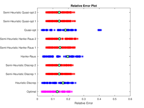
Figure 1: Tomography operator perturbed by random operator: $D=600$ for SH1, $D=0.05$ for SH2 and $\gamma=0.005\times\eta$.

We see that the semi-heuristic rules present a noticeable improvement for all parameter choice rules, although the discrepancy in performance seems to be slightly more pronounced for the quasioptimality and Hanke-Raus rules.

We also compare the difference between the values of $e_{\text{per}}$ with respect to the modified parameter choice rule and its unmodified counterpart, respectively as a percentage. For example, for any configuration of data and operator noise, we would compute the value

$$\theta(\delta,\eta)=(e_{\text{per}}-\bar{e}_{\text{per}})\times 100,$$ (22)

where $e_{\text{per}}$ and $\bar{e}_{\text{per}}$ denote the error ratio for the standard heuristic rule (i.e., $D=0$ and $\alpha_{\text{min}}=\lambda_{\text{min}}$) and the modified rule (11) or (12), respectively. This value is computed for several noise-levels $\delta$ and operator error levels $\eta$. Note that positive values indicate that the semi-heuristic rules outperform their heuristic counterparts and vice versa.

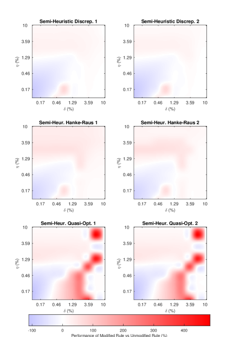
Figure 2: Tomography operator perturbed by random operator: set-up identical to Figure 1. Red indicates that the semi-heuristic rules perform better than their standard heuristic counterparts and vice versa.

The plots of Figure 2 indicate that the semi-heuristic rules do not necessarily offer improvements for small data and operator noise, but exhibit increased performance for larger noise of both aforementioned varieties. In particular, this is more pronounced for the quasioptimality rule where we may observe blotches of dark red which indicate significant improvement over the standard heuristic rule.

The standard heuristic rules also performed reasonably well and a possible explanation could be the argumentation for the use of the compensating functional was based on the regularity of the operator noise and therefore it is probable that the irregularity of the operator noise in this scenario did not aid the premise of using the modified rules.

3.2 Smooth Operator Perturbation

Fredholm integral operator perturbed by heat operator

To simulate a deterministic, possibly smooth, operator perturbation, we first consider the Fredholm integral operator of the first kind perturbed by a heat operator, which we think is an instance where the noise condition for $A_{\eta}$ might fail and where a semi-heuristic modification is highly advisable.

For the implementation, we use the baart and heat packages on Hansen’s Regularization Tools to define the finite dimensional operator $A_{\eta}\in\mathbb{R}^{n\times n}$, with $n=400$, where $A_{\eta}=A+C\Delta A$ is the superposition of the baart operator and scaled heat operator, respectively. More precisely, the baart operator is the discretisation of a Fredholm integral equation of the first kind with kernel $K_{1}:(s_{1},t_{1})\mapsto\exp(s_{1}\cos t_{1})$, where $s_{1}\in[0,\pi/2]$, $t_{1}\in[0,\pi]$, and the heat operator is taken to be the Volterra integral operator with kernel $K_{2}:(s_{2},t_{2})\mapsto k(s_{2}-t_{2})$, where

$$k(t):=\frac{t^{-\frac{3}{2}}}{2\sqrt{\pi}}\exp\left(-\frac{1}{4t}\right),$$

for $t\in[0,1]$. The exact solution is given by $y(s)=2\sin s/s$ and the data noise is defined as before.

We proceed similarly as in the previous experiment.

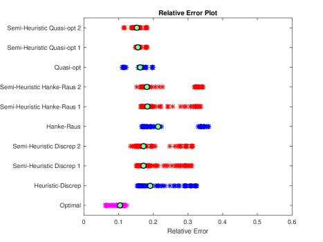
Figure 3: Fredholm operator of the first kind perturbed by heat operator: $D=600$ for SH1, $D=0.12$ for SH2 and $\gamma=0.07\times\eta$.

In Figure 3, we observe that the best performing rule is in fact the semi-heuristic quasioptimality rule (SH1). The semi-heuristic variants of the Hanke-Raus and heuristic discrepancy rules are also improvements on the original rules, although this is slightly more pronounced for the semi-heuristic Hanke-Raus rules.

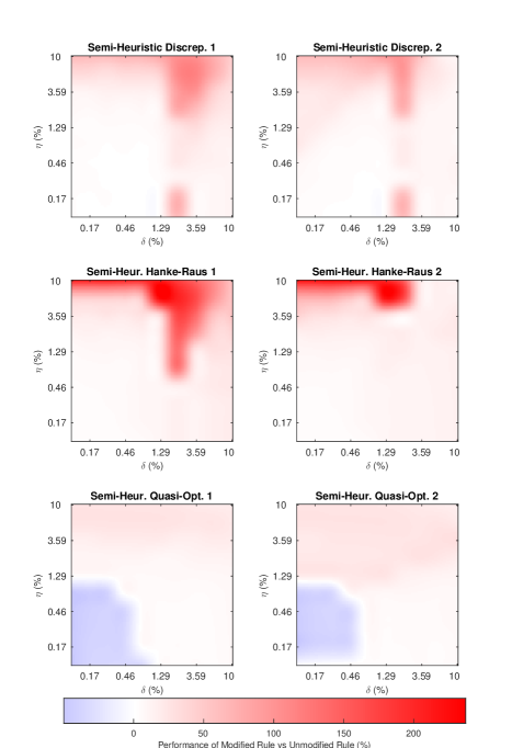
Figure 4: Fredholm operator of the first kind perturbed by heat operator: set-up identical to Figure 3. Red indicates that the semi-heuristic rules perform better than their standard heuristic counterparts and vice versa.

In Figure 4, the plots for the heuristic discrepancy and Hanke-Raus rules demonstrate that the semi-heuristic rules offer an overall improvement for all ranges of operator and data noise. However, we observe that the semi-heuristic quasioptimality rules performs slightly worse for small data and operator noise, but exhibit much better performance when both the mentioned noises are larger. Additionally, one may also observe that the semi-heuristic Hanke-Raus rules perform significantly better than their standard heuristic counterparts for very large operator noise.

Blur operator perturbed by tomography operator

In a next experiment, we again simulate a deterministic operator perturbation by considering the blur operator from Hansen’s tools and perturbing it by the tomography operator from before. For the blur operator, we set $\texttt{band}=8$ and $\texttt{sigma}=0.9$, which is modelled by the Gaußian point spread function:

$$h(x,y)=\frac{1}{2\pi\sigma^{2}}\exp\left(-\frac{x^{2}+y^{2}}{2\sigma^{2}}\right).$$

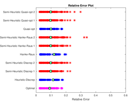
Figure 5: Blur operator perturbed by tomography operator: $D=500$ for SH1, $D=0.2$ for SH2 and $\gamma=0.01\times\eta$.

In Figure 5, we observe as before that the semi-heuristic rules exhibit improvements over their standard counterparts for the heuristic discrepancy and Hanke-Raus rules, although the standard quasioptimality rule performs quite well and in this case, its semi-heuristic variants do not necessarily present a better choice.

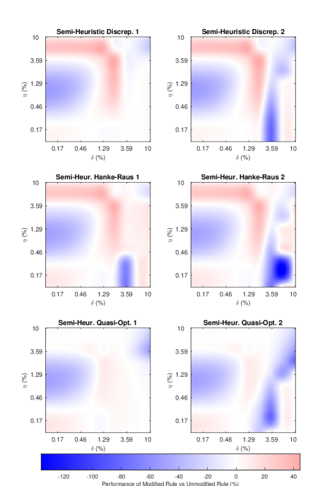
Figure 6: Blur operator perturbed by tomography operator: set-up identical to Figure 5. Red indicates that the semi-heuristic rules perform better than their standard heuristic counterparts and vice versa.

In Figure 6, it is difficult to draw any meaningful conclusions, although it seems that for large operator noise and reasonable data noise, the semi-heuristic discrepancy and Hanke-Raus rules perform better than the standard heuristic rules. Consequently, one may conclude that for many situations, the semi-heuristic rules offer an improvement on their standard heuristic counterparts.

Note that in all experiments, the minimiser in the range $[\lambda_{\text{min}},\alpha_{\text{max}}]$ of the standard heuristic functionals was occasionally $\alpha_{\text{max}}$; particularly when the operator noise was large. Note that we rectified this failure by the interior minima search as described above. Had we not rectified this failure, the improvement of the semi-heuristic methods would have been even greater pronounced.

4 Conclusion

In this paper, we presented a modification of the standard heuristic parameter choice rules in the case of a known bound on the operator perturbation but unknown data noise-level. In particular, the modifications were two-fold: the introduction of a compensating function and an appropriately selected lower bound, the motivations for which have been covered.

We proved convergence of the modified rules as the data and operator errors tend to zero provided that the noise condition holds and the lower bound of the regularisation parameter satisfies certain condition.

The numerical experiments confirmed that the semi-heuristic methods may yield an improvement over the standard parameter choice rules in many situations. Incidentally, the optimal choices of $D$ and $\gamma$ presents room for further research.

References

[1]A. Bakushinskiy, Remarks on choosing a regularization parameter
using quasi-optimality and ratio criterion, USSR Computational Mathematics
and Mathematical Physics, 24 (1985), pp. 181–182.
[2]F. Bauer and M. A. Lukas, Comparing parameter choice methods for
regularization of ill-posed problems, Math. Comput. Simulation, 81 (2011),
pp. 1795–1841.
[3]H. Engl, M. Hanke, and A. Neubauer, Regularization of Inverse
Problems, Mathematics and Its Applications, Springer Netherlands, 1996.
[4]U. Hämarik, R. Palm, and T. Raus, On minimization strategies for
choice of the regularization parameter in ill-posed problems, Numerical
Functional Analysis and Optimization, 30 (2009), pp. 924–950.
[5]U. Hämarik, R. Palm, and T. Raus, Comparison of parameter choices
in regularization algorithms in case of different information about noise
level, Calcolo, 48 (2011), pp. 47–59.
[6]M. Hanke and P. C. Hansen, Regularization methods for large-scale
problems, Surveys Math. Indust., 3 (1993), pp. 253–315.
[7]M. Hanke and T. Raus, A general heuristic for choosing the
regularization parameter in ill-posed problems, SIAM Journal on Scientific
Computing, 17 (1996), pp. 956–972.
[8]P. C. Hansen, Regularization tools: a Matlab package for analysis
and solution of discrete ill-posed problems, Numer. Algorithms, 6 (1994),
pp. 1–35.
[9]S. Kindermann, Convergence analysis of minimization-based noise
level-free parameter choice rules for linear ill-posed problems, Electron.
Trans. Numer. Anal., 38 (2011), pp. 233–257.
[10]S. Kindermann and A. Neubauer, On the convergence of the
quasioptimality criterion for (iterated) Tikhonov regularization, Inverse
Problems and Imaging, 2 (2008), pp. 291–299.
[11]S. Kindermann, S. Pereverzyev Jr., and A. Pilipenko, The
quasi-optimality criterion in the linear functional strategy, Inverse
Problems, (2018), p. 075001.
[12]M. A. Krasnoselskiĭ, P. P. Zabreĭ ko, E. I. Pustylnik, and P. E.
Sobolevskiĭ, Integral operators in spaces of summable functions,
Noordhoff International Publishing, Leiden, 1976.
Translated from the Russian by T. Ando, Monographs and Textbooks on
Mechanics of Solids and Fluids, Mechanics: Analysis.
[13]S. Lu, S. V. Pereverzev, and U. Tautenhahn, Regularized total least
squares: Computational aspects and error bounds, SIAM J. Matrix Anal. Appl.,
31 (2009), pp. 918–941.
[14]S. Lu, S. Pereverzyev, Y. Shao, and A. U Tautenhahn, On the
generalized discrepancy principle for Tikhonov regularization in Hilbert
scales, Journal of Integral Equations and Applications - J INTEGRAL EQU
APPL, 22 (2010).
[15]T. Raus and U. Hämarik, On the quasi-optimal rules for the
choice of the regularization parameter in case of a noisy operator, Advances
in Computational Mathematics, 36 (2012), pp. 221–233.
[16]T. Raus and U. Hämarik, Heuristic parameter choice in Tikhonov
method from minimizers of the quasi-optimality function, In: Hofmann B.,
Leitão A., Zubelli J. (eds) New Trends in Parameter Identification for
Mathematical Models. Trends in Mathematics. Birkhäuser, Cham, (2018),
pp. 227–244.
[17]U. Tautenhahn, Regularization of linear ill-posed problems with
noisy right hand side and noisy operator, Journal of Inverse and Ill-posed
Problems - J INVERSE ILL-POSED PROBL, 16 (2008), pp. 1–17.
[18]A. Tikhonov and V. Glasko, The approximate solution of Fredholm
integral equations of the first kind, USSR Computational Mathematics and
Mathematical Physics, 4 (1969), p. 236–247.
[19]G. M. Vaĭ nikko and A. Y. Veretennikov, Iteratsionnye protsedury
v nekorrektnykh zadachakh, “Nauka”, Moscow, 1986.