Conditional Masking to Numerical Data

Abstract

Protecting the privacy of data-sets has become hugely important these days. Many real-life data-sets like income data, medical data need to be secured before making it public. However, security comes at the cost of losing some useful statistical information about the data-set. Data obfuscation deals with this problem of masking a data-set in such a way that the utility of the data is maximized while minimizing the risk of the disclosure of sensitive information. Two popular approaches to data obfuscation for numerical data involves (i) data swapping and (ii) adding noise to data. While the former masks well sacrificing the whole of correlation information, the latter gives estimates for most of the popular statistics like mean, variance, quantiles, correlation but fails to give an unbiased estimate of the distribution curve of the original data. In this paper, we propose a mixed method of obfuscation combining the above two approaches and discuss how the proposed method succeeds in giving an unbiased estimation of the distribution curve while giving reliable estimates of the other well-known statistics like moments, correlation.

1 Introduction

Estimation of statistics like mean, variance, quantiles is fundamental for statistical analysis of data. But, if the data is sensitive to the individual bearing the information, it may be almost impossible to publish the data in its raw form. Data obfuscation calls for methods that can protect the individual information from any possible intruder while retaining as much statistical utility as possible. The two motives of data obfuscation are

1. Maximising data utility

2. Minimising risk of disclosure.

A typical data-set we are thinking of consists of $m$ variable values corresponding to $n$ individuals and among these $m$ variables one or a few variables have some sensitive information related to the individual. One may think, at first, that if the name or identification number of the individual is erased, there is no point in protecting the values as the intruder would not know who this value belongs to. But, in reality, the scenario is different from this intuitive belief. In many cases, even if the identification information is not given, looking at all the variable values in the row, the intruder often becomes successful in identifying the individual. The paper [7] discusses how the presence of a few non-sensitive attributes may jointly disclose the identity of an individual in a data-set consisting of several attributes. For example, in an official data-set, age-group, sex, birthplace may not individually leak the identity of an individual but suppose, it is known to the intruder that there is only one male in the data-set with age group 20-25 who comes from “Kerala”. Then jointly, these three attribute values will reveal the identity of the individual. Thus, practically, it is often very difficult to hide the identity of the individual in presence of many attributes. Moreover, in many practical cases, the identifier may be an essential attribute. Thus, the sensitive attributes, i.e., the ones that carry values that shall not be disclosed as for example income data, marksheet data etc. needs protection.

As an early reference one can go through the papers of Steinberg and Pritzker ( 1967) [1] Bachi and Banon ( 1969) [2] that discusses the importance of privacy protection in the case of sensitive data. Dalenius ( 1974)[3] discussed the importance of the disclosure problem in statistical studies. Mugge (1983) [5] discussed the issues in protecting confidentiality in National Health Statistics. Dalenius ( 1977a)[4] Fienberg ( 1994)[6] discusses the importance of the problem in Computers and individual privacy.

There are various methods of obfuscating data as discussed in [8][9][11][10]. Two of them involve swapping the data values among them and adding noise to individual values. While in a large data-set if values corressponding to only one sensitive variable are swapped, it does not harm the estimates of mean, variance, moments or quantiles for the data but, its correlation information with any other variable is completely erased after swapping. This gave rise to methods like rank swapping as discussed by Moore( 1996) in [11], and data shuffling by R. Sarathy and K. Muralidhar in [12]. To get satisfactory estimates after rank swapping, the disclosure risk gets very high. Hence, this method often fails to perform well. Data shuffling is a more reliable method of obfuscation; it shuffles the data in such a way that the correlation between variables is not harmed, but in case there are a large number of variables it may become impossible or much more tedious to shuffle even the non-sensitive variables to retain their correlation information with the sensitive one.

Adding noise to data, on the other hand, gives us estimates of the mean, variance and quantiles without doing much harm to the correlation information. But after sufficient obfuscation, there may be a considerable amount of loss of utility of the data. Also, there is no known procedure to get an unbiased estimation of the distribution curve in this model which makes quantile estimation, a hard problem.

In this paper, we introduce a new approach to data obfuscation, a method that combines data swapping and addition of noise. Here, a part of the data is swapped and to the rest of the data, we add noise from a normal distribution with mean zero and known variance. The resulting data in hand will be useful in giving an unbiased estimation procedure to the distribution curve of the original data resulting in very good quantile estimates while giving sufficient masking to the data values.

In Section 2, we discuss the basic model of the procedure, estimate the disclosure risk and also some useful statistics with the required proofs in the Appendix section. In Section 3, we simulate a data-set of size 2000 and apply our procedure to the given problem to see check how our process works. Also, a simulation study is given to see how the process works for increasing sample size. In Section 4, we apply the procedure to a real-life problem, a data-set of marks of 445 students of an institute and see how after sufficient obfuscation our procedure gives reliable estimates of various statistics, especially the quantiles. Finally, we conclude with some discussions in Section 5.

2 Basic Problem

Suppose we have a large data-set with $m$ variables, corresponding to $n$ individuals; and among these $m$ variables, there is some numerical variable which is sensitive and needs to be protected. Let the data values corresponding to this variable be $\{X_{i},1\leq i\leq n\}$, which is assumed to come from some unknown distribution function $\{G(x),x\in R\}$ which is continuous. The idea is to obfuscate the data in a way such that with some probability $p$ the obfuscated value $Z_{i}$ corresponding to $X_{i}$ takes any other value among $\{X_{i},1\leq i\leq n\}$ expect $X_{i}$ and with probability $1-p$ it adds a noise to the data values. To perform this method, we first simulate $\{B_{i},1\leq i\leq n\}$ independent of $\{X_{i},1\leq i\leq n\}$ where $B_{i}$ is a $Bin(1,p)$ variable, i.e, a binary variable with probability of success $p$. The obfuscated data $\{Z_{i},1\leq i\leq n\}$ then looks like the following

$$Z_{i}=\left\{\begin{array}[]{lr}X_{j}&\mbox{ $j\neq i$, if $B_{i}=1$ }\\ X_{i}+Y_{i}&\mbox{if $B_{i}=0$}\end{array}\right.$$ (1)

where $Y_{i}\sim N(0,\sigma^{2})$, $\sigma$ is known, $1\leq i\leq n$, and $j$ is chosen randomly from the set $\{\{1,2,\ldots,n\}\backslash\{i\}\}$ randomly, i.e., with probability $\frac{1}{n-1}$.

Note that $\{Z_{i},1\leq i\leq n\}$ is a set of independent variables, each data point $Z_{i}$ being dependent on $X_{i}$ and $B_{i}$ but not on each other. However, two $Z_{i}$s may take the same value but usually with a very low probability for large value of $n$. Hereafter, we will discuss the estimation of the raw moments( mean and variance especially) and quantiles of $X$ from the knowledge of $\{Z_{i},1\leq i\leq n\}$, $p$ and $\sigma$, its correlation with any other variable $X^{\prime}$ and also about the disclosure risk associated with such model. Usually, Laplace noise is used in additive noise model but here we use Normal error because under this model, estimation would become very hard for any other distribution of noise other than Normal.

2.1 Estimation of Moments

A fundamental problem in statistics is to estimate the moments of a data set especially the mean and variance. Here, we will see that even after sufficient obfuscation it is possible to get reliable estimates for the raw moments of the true data using the following theorem. Once we find the raw moments, central moments can be easily derived using the standard relation between moments.

Theorem 2.1.

If $\{X_{i},1\leq i\leq n\}$ is assumed to be an i.i.d. sample from some unknown distribution function $G(x)$ ( $G$ is a continuous function) with finite absolute raw moments, i.e.,

$$E(|X_{i}|^{k})<\infty\mbox{ , $\forall$ $k\in N$}.$$

and $\{Z_{i},1\leq i\leq n\}$ is obtained using Equation (1), then an unbiased estimator for the $k^{th}$ raw moment of $X$ ( $X\sim G(.)$, $k\in N$) is obtained from the recursion relation given below

$$\hat{\mu}_{(X,k)}=\hat{\mu}_{(Z,k)}-(1-p)\cdot({\mu}_{(Y,k)}+\binom{k}{1}\cdot{\mu}_{(Y,k-1)}\cdot\hat{\mu}_{(X,1)}+\cdots+\binom{k}{k-1}\cdot\hat{\mu}_{(X,k-1)}\cdot{\mu}_{(Y,1)})$$

where, $\hat{\mu}_{(X,1)}=\bar{Z}$, $\hat{\mu}_{(Z,k)}=\frac{1}{n}\cdot\sum_{j=1}^{n}{Z_{j}^{k}}$,

$$\begin{array}[]{lr}{\mu}_{(Y,k)}&=\mbox{$k^{th}$ raw moment of $N(0,\sigma^{2})$}\\ &=\left\{\begin{array}[]{lr}0&\mbox{ $k$ is odd }\\ {\frac{\sigma^{k}\cdot k!}{2^{k/2}\cdot{k/2}!}}&\mbox{ $k$ is even.}\end{array}\right.\end{array}$$

From Theorem 2.1, we have $\bar{Z}$ to be an unbiased estimate of $\mu_{X}$, mean of $X$.

Also, we have,

$$\begin{array}[]{lr}\hat{\mu}_{(X,2)}&=\hat{\mu}_{(Z,2)}-(1-p)\cdot({\mu}_{(Y,2)}+2\cdot{\mu}_{(Y,1)}\cdot\mu_{X})\\ &=\hat{\mu}_{(Z,2)}-(1-p)\cdot\sigma^{2}\end{array}$$

Define, $\hat{S}_{X}^{2}=\hat{S}_{Z}^{2}-(1-p)\cdot\sigma^{2}$ where ${\hat{S}_{Z}^{2}=\frac{1}{n-1}\sum_{i=1}^{n}{(Z_{i}-\bar{Z})^{2}}}$.

$$E(\hat{S}_{X}^{2})=\sigma_{Z}^{2}-(1-p)\cdot\sigma^{2}=\sigma_{X}^{2}\mbox{ , where ${\sigma_{X}^{2}=Var(X_{1}),\sigma_{Z}^{2}=Var(Z_{1})}$}$$

2.2 Estimation of Quantiles

In non-parametric studies, the estimation of the median, or in general, any quantile is most crucial. Moreover, quantiles are robust statistics and hence is not much affected by the presence of outlying data-points. To do the same we first estimate the c.d.f. of $X$ from the model using the following Theorem.

Theorem 2.2.

If $\{X_{i},1\leq i\leq n\}$ is assumed to come from some unknown d.f. $\{G(x),x\in R\}$ and $\{Z_{i},1\leq i\leq n\}$ is obtained using Equation (1) then, for $p>0.5$,

$$T_{1}(x)=\frac{1}{np}\sum_{j=1}^{n}{\sum_{t=0}^{\infty}{\lambda^{t}\cdot\Phi_{\sigma\sqrt{t}}(x-Z_{j})}}$$ (2)

is an unbiased estimator for $G(x)$ $\forall x\in R$ , where $\lambda=-\frac{1-p}{p}$ and $\Phi_{m}(i)$ is the cumulative distribution function of a Normal variable at $i$ with mean 0 and standard deviation $m$ for $m>0$ and for $m=0$, $\Phi_{0}(i)=\mathbb{I}(x-Z_{j})$ where $\mathbb{I}(i)=1$ if $i\geq 0$ and $0$ o.w.

Although Theorem 2.2 gives us an u.e. for $G(x)$, this estimator will give good results only for very large $n$. If $n$ is large but not very large, then sometimes the estimator we get to look at in the following Theorem may give us a smooth estimate to the curve of $G(x)$, i.e., $\hat{G}(x)$ is a smooth function or a function that has derivatives of all orders everywhere in its domain.

Theorem 2.3.

If $\{X_{i},1\leq i\leq n\}$ is assumed to come from some unknown distribution function $\{G(x),x\in R\}$, having a density function, and $\{Z_{i},1\leq i\leq n\}$ is obtained using Equation (1) then, for $p>0.5$,

$$T_{b}(x)=\frac{1}{np}\sum_{j=1}^{n}{\sum_{t=0}^{\infty}{\lambda^{t}\cdot\Phi_{b_{t}}(x-Z_{j})}}$$ (3)

is a smooth estimator for $G(x)$ $\forall x\in R$ , where $\lambda=-\frac{1-p}{p}$, $b_{t}=\sqrt{tb^{2}+\sigma^{2}}$ and $\Phi_{\upsilon}(i)$ is the cumulative distribution function of a Normal variable at $i$ with mean 0 and standard deviation $\upsilon$.

The estimator $T_{1}(x)$ is unbiased while $T_{b}(x)$ is not but is smooth and sometimes more useful than the former. However, we study the asymptotic properties of such estimators in the following theorem.

Theorem 2.4.

Both the estimators $T_{1}(x)$ and $T_{b}(x)$ are the mean of i.i.d. random variables with finite expectation and variances and are consistent in the sense

$$T_{i}(x)\overset{P}{\longrightarrow}G(x)\mbox{ , $\forall x$ as $n\rightarrow\infty$ , $i=1,b$}$$

To estimate the $\alpha^{th}$ quantile, we equate $\hat{G}(x)$ instead of $G(x)$ with $\alpha\in(0,1)$ using some numerical method, i.e., $\hat{\xi_{\alpha}}$ is such that

$$\hat{G}(\hat{\xi_{\alpha}})=\alpha$$

2.3 Estimation of correlation

While swapping of data values among them retains the exact information of the mean, variance and quantiles, it does completely erase any possible correlation information of the variable with any other variable. That is why additive noise model is used while obfuscating a single sensitive variable among many. However, our method gives us a reasonable estimate for the correlation coefficient.

Theorem 2.5.

Let $\{X^{\prime}_{i},1\leq i\leq n\}$ be the data points corresponding to some variable $X^{\prime}$ associated with $X$, correlation coefficient between $X$ and $X^{\prime}$ being $\rho_{(X,X^{\prime})}$. Then, if the variance of $X$ and $X^{\prime}$ exists and is finite and so is $d(X,X^{\prime})=E[(X-E(X))^{2}(X^{\prime}-E(X^{\prime}))^{2}]$,

$$\hat{\rho}_{(X,X^{\prime})}=\frac{1}{1-p}\cdot\frac{\hat{Cov}(Z,X^{\prime})}{\sqrt{\hat{Var}(X^{\prime})}\cdot\sqrt{\hat{Var}(X)}}$$

is a consistent estimator of $\rho$ where $\hat{Cov}(Z,X^{\prime})=\frac{1}{n}\cdot[\sum_{j=1}^{n}{Z_{j}\cdot X^{\prime}_{j}}-\bar{Z}\cdot\bar{X^{\prime}}]$.

2.4 Disclosure Risk

In data obfuscation, estimation is important but not at the cost of disclosure of data values. So to check the disclosure risk of data, obfuscated with this method, note that the possible estimators for $X_{i}$ from the available information of obfuscated data are $Z_{i}$ and $\bar{Z}$, both being unbiased estimators of $X_{i}$. $\bar{Z}$ can be shown to be a better estimator of $X_{i}$ than $Z_{i}$, as long as the minimum MSE is concerned, which means we get one estimate for each $X_{i}$ which is possibly its best estimator. Hence, the disclosure risk is not expected to be high for medium to large values of $n$.

$$MSE(Z_{i})=E(Z_{i}-X_{i})^{2} = \frac{p}{n-1}\cdot\sum_{j=1}^{n}{E(X_{i}-X_{j})^{2}}+(1-p)\cdot E(Y_{i}^{2})$$

$$= 2p\cdot\frac{n}{n-1}\sigma_{X}^{2}+(1-p)\cdot\sigma^{2}$$

$\begin{array}[]{ll}MSE(\bar{Z})&=E(\bar{Z}-X_{i})^{2}\\ &=E((\bar{Z}-E(X))-(X_{i}-E(X)))^{2}\\ &=E(\bar{Z}-E(X))^{2}+E(X_{i}-E(X))^{2}-2E(\bar{Z}-E(X))(X_{i}-E(X))\\ &=\sigma_{X}^{2}+\frac{p\sigma_{X}^{2}+(1-p)\sigma^{2}}{n}-2\frac{\sigma_{X}^{2}}{n}\\ &=\sigma_{X}^{2}(1-\frac{2-p}{n})+\frac{1-p}{n}\sigma^{2}\\ &\leq MSE(Z_{i})\mbox{ , since $2p\frac{n}{n-1}>1$ and $0\leq\frac{2-p}{n}\leq 1$ for $n>1$.}\end{array}$

Thus, $\bar{Z}$ is a better estimator of $X_{i}$ than $Z_{i}$ for all $n>1$ as far as MSE is concerned. However, the disclosure risk for any estimator $\tau$ for $X_{i}$ can be measured by,

$$P[|\tau-X_{i}|<d]\mbox{ , for $d>0$}$$

i.e., the probability that $X_{i}$ lies within a $d$-boundary of its estimator. This measure was used in our previous work as discussed in [13]. For $S$ simulations, an estimate of risk is given by,

$$\frac{\sum_{s=1}^{S}{I_{[\tau_{s}\in(X_{i}-d,X_{i}+d)]}}}{S}$$

where $\tau_{s}$ is the estimate of $X_{i}$ for $s^{th}$ simulation and $I_{[A]}=1$ if event $A$ occurs and $0$ otherwise.

3 Simulation Results

To apply the discussed method we simulate a sample of dimension $n\times 2$ for a given copula structure using the function mvdc in package copula of R 3.3.2. We take $n=2000$ and a copula structure such that the first variable is from Laplace($\mu_{1}=10$,$\sigma_{1}=1000$), the second variable from Laplace($\mu_{2}=50$,$\sigma_{2}=250$) and the correlation between these two variables is $\rho=-0.7$. Of the two samples of size $n$, we consider the first one to be the sensitive variable and the other one the variable correlated with the sensitive one. Now we obfuscate the sensitive variable, say, $\{X_{i},1\leq i\leq n\}$ with the method discussed (Equation (1)) to get the obfuscated variable $\{Z_{i},1\leq i\leq n\}$; we used $\sigma=\sigma_{1}$. Also, to compare the method with the general additive noise model, we also obfuscate $\{X_{i},1\leq i\leq n\}$ with addition of noise $\{Y_{1i},1\leq i\leq n\}$, $Y_{1i}\sim Laplace(0,\tilde{\sigma}^{2})$ to get $\{Z_{1i},1\leq i\leq n\}$. Note that, the noise is taken from Laplace because we need to estimate the quantiles from the obfuscated data and as discussed in our previous work [13], Laplace is till now the best possible choice for the obfuscating distribution. To keep the dispersion of the variables more or less same, we take $\tilde{\sigma}=\sigma_{1}$, although this is just a choice; in general, the method works well when the estimation of quantiles is needed from a large data-set with low disclosure risk. The method of obfuscation also works well for lower values of $\sigma$.

Figure 1 shows the true distribution curve $G(x)$ and estimates of ${G(x)}$ from the obfuscated data-sets as discussed in the previous paragraph. Table 1 shows the true and estimated values of the quantiles for $\alpha=\{0.1,0.2,0.3,0.4,0.5,0.6,0.7,0.8,0.9\}$ and also that of the mean, variance and correlation with the other variable for the same data-set. Although theoretically we only have $p>0.5$, a very high value of $p$ tends to make the procedure a data swapping process which completely erases the correlation information. Thus, throughout this section, we will take $p=0.6$.

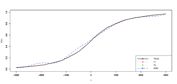
Figure 1: True and estimated distribution curve using Additive Noise Model and our method for simulated data

Table 1: Estimated Statistics from original and obfuscated data using additive noise model and our method for simulated data.

Statistic	TRUE	T1	Tb	ANM
0.1	-1599.438	-1720.259	-1768.946	-1818.652
0.2	-906.291	-942.292	-983.028	-1147.267
0.3	-500.826	-479.118	-545.852	-619.269
0.4	-213.144	-191.17	-217.001	-255.806
0.5	10	71.045	53.987	37.518
0.6	233.144	296.573	313.607	337.252
0.7	520.826	544.369	600.41	679.548
0.8	926.291	924.456	976.201	1123.431
0.9	1619.438	1631.023	1631.599	1814.377
Mean	10	10.27	10.27	10.834
s.d.	1414.214	1442.762	1442.762	1444.929
Cor	-0.7	-0.745	-0.745	-0.69

Looking at the graph, one can easily notice that the curves we get using $T_{1}$ and $T_{b}$ are comparatively closer to the cumulative distribution functions of $X$ than the one we get using the Additive Noise Model. Also, from the table we see the quantile estimates are improved from the Additive Noise Model without doing much harm to the mean, variance or correlation information. However, a single simulation does not show much insight to a process. So, we repeat the process $S$ times and found the estimates of bias and root mean-squared error for $S=\{500,800,1000\}$ [See Table 3 and 4].

Note that the values for different $S$ remain more or less same which means the bias and r.m.s.e. are consistent. One can now easily observe that the moments and correlation are well-estimated in both additive noise model and this method. However the quantile estimates are improved to a remarkable extent. Even for this large value of $\sigma$, this method still gives reliable estimate for the same. However, a reliable estimate is only relevant if the data is well protected against disclosure. To measure the disclosure risk we calculate the value of the statistic $\frac{\sum_{s=1}^{S}{I_{[\tau_{s}\in(X_{i}-d,X_{i}+d)]}}}{S}$ for $\tau=Z_{i}$ (as shown in Table 2), assuming $Z_{i}$ to be the best estimator of $X_{i}$.

Table 2: Disclosure risk for Additive Noise Model and our method for $S=1000$ simulations for simulated data

d	CM	ADM
250	0.153	0.221
500	0.298	0.393
1000	0.541	0.632
1500	0.712	0.777
2000	0.819	0.864

Note:The simulated values were same for $S=$ 500,800 and 1000.

One can easily observe that the average number of $Z_{i}$ that lies within $d$-boundary of $X_{i}$ is very small for average $d$. Even for $d$ as large as the dispersion of $X$, it is about $55\%$ for Conditional Masking and $60\%$ for Additive Noise Model. Hence the data is well masked for both the procedures however conditional masking gives even better result than additive noise model.

To illustrate consistency of the estimators we also simulate data-sets for increasing $n$. We calculate the bias, r.m.s.e. and disclosure risk values for $n=\{2000,5000,10000\}$ [See Table 5 and 6].

Looking at the tables one can easily see that the bias and r.m.s.e. for both the estimators decrease for increasing $n$ which shows numerically that the estimators are consistent.

Note

We only compare the results of Additive Noise Model (ADM) and our method but not data swapping, because a simple data swapping would result in exact estimates for mean, variance and quantiles, and complete loss of information in correlation information.

Table 3: Estimated bias from original and obfuscated data using additive noise model and our method for simulated data

Statistic		0.1	0.2	0.3	0.4	0.5	0.6	0.7	0.8	0.9	Mean	s.d.	Cor
TRUE		-1599.438	-906.291	-500.826	-213.144	10	233.144	520.826	926.291	1619.438	10	1414.214	-0.7
$T1$	$S=500$	-7.451	2.401	2.102	-1.863	0.521	0.432	2.108	2.427	6.227	0.775	2.323	0.017
	$S=800$	-8.471	-2.942	-1.879	-3.991	-1.4	-0.642	-0.442	0.144	3.795	-1.614	1.474	0.014
	$S=1000$	-7.352	-1.811	-0.905	-3.454	-1.258	-0.563	0.247	1.462	5.063	-0.867	0.823	0.014
$Tb$	$S=500$	-45.966	-38.447	-38.614	-30.765	0.246	31.645	41.11	42.056	44.454	0.775	2.323	0.017
	$S=800$	-47.689	-43.033	-41.884	-33.153	-1.689	29.832	39.034	40.259	42.477	-1.614	1.474	0.014
	$S=1000$	-46.583	-41.949	-41.176	-32.686	-1.434	29.986	39.394	41.137	44.209	-0.867	0.823	0.014
$ANM$	$S=500$	-94.454	-80.728	-71.085	-45.791	4.934	54.31	76.414	87.079	97.813	3.775	1.188	0.014
	$S=800$	-91.866	-81.986	-73.177	-47.933	3.475	53.422	75.265	82.036	88.739	0.677	0.508	0.012
	$S=1000$	-90.616	-81.279	-73.082	-48.576	2.916	53.972	77.217	84.69	88.395	1.858	0.369	0.013

Table 4: Estimated R.M.S.E. from original and obfuscated data using additive noise model and our method for simulated data

Statistic		0.1	0.2	0.3	0.4	0.5	0.6	0.7	0.8	0.9	Mean	s.d.	Cor
TRUE		-1599.438	-906.291	-500.826	-213.144	10	233.144	520.826	926.291	1619.438	10	1414.214	-0.7
$T1$	$S=500$	105.718	68.505	54.114	42.623	36.512	41.823	53.924	76.498	111.902	43.763	49.925	0.068
	$S=800$	107.288	71.566	54.496	43.241	36.921	43.596	54.859	75.663	112.72	45.169	50.679	0.068
	$S=1000$	107.782	72.018	55.38	43.688	37.324	43.612	54.631	75.574	111.266	45.644	51.006	0.068
$Tb$	$S=500$	104.803	76.242	63.377	51.001	36.652	49.97	62.705	77.296	107.898	45.169	50.679	0.068
	$S=800$	104.803	76.242	63.377	51.001	36.652	49.97	62.705	77.296	107.898	45.169	50.679	0.068
	$S=1000$	105.643	76.396	63.453	51.097	36.886	50.12	62.905	77.537	107.897	45.644	51.006	0.068
$ANM$	$S=500$	190.174	134.445	105.501	78.966	62.894	85.24	108.607	138.752	190.351	43.877	57.674	0
	$S=800$	191.034	134.439	107.09	80.88	62.741	83.996	106.855	136.38	185.941	45.013	57.753	0
	$S=1000$	192.051	133.318	106.236	81.216	62.656	85.37	109.275	136.992	186.095	44.98	57.573	0

Table 5: Estimated bias from obfuscated data using additive noise model and our method for simulated data

Statistic		0.1	0.2	0.3	0.4	0.5	0.6	0.7	0.8	0.9	Mean	s.d.	Cor
Original		-1599.438	-906.291	-500.826	-213.144	10	233.144	520.826	926.291	1619.438	10	1414.14	-0.7
$T1$	$n=2000$	-7.352	-1.811	-0.905	-3.454	-1.258	-0.563	0.247	1.462	5.063	18.791	-21.263	0.04
	$n=5000$	-1.588	0.801	0.751	0.796	1.349	0.745	1.43	0.945	1.799	-15.926	8.02	0.068
	$n=10000$	0.795	1.277	0.978	0.582	0.542	0.633	0.301	1.147	1	19.138	15.358	0.045
$Tb$	$n=2000$	-46.583	-41.949	-41.176	-32.686	-1.434	29.986	39.394	41.137	44.209	18.791	-21.263	0.04
	$n=5000$	-28.755	-27.651	-27.321	-22.492	1.039	24.445	29.197	29.306	29.454	-15.926	8.02	0.068
	$n=10000$	-20.704	-20.347	-20.296	-17.855	0.67	19.148	21.835	22.358	22.539	19.138	15.358	0.045
$ANM$	$n=2000$	0.795	1.277	0.978	0.582	0.542	0.633	0.301	1.147	1	19.138	15.358	0.045
	$n=5000$	-20.704	-20.347	-20.296	-17.855	0.67	19.148	21.835	22.358	22.539	19.138	15.358	0.045
	$n=10000$	-41.152	-42.353	-38.741	-30.838	0.355	31.815	40.871	44.796	40.295	18.227	16.06	0

Table 6: Estimated R.M.S.E. from obfuscated data using additive noise model and our method for simulated data

Statistic		0.1	0.2	0.3	0.4	0.5	0.6	0.7	0.8	0.9	Mean	s.d.	Cor
Original		-1599.438	-906.291	-500.826	-213.144	10	233.144	520.826	926.291	1619.438	10	1414.14	-0.7
$T1$	$n=2000$	107.782	72.018	55.38	43.688	37.324	43.612	54.631	75.574	111.266	45.644	418.158	0.068
	$n=5000$	68.685	46	35.846	27.968	23.005	27.244	34.355	45.338	68.205	28.834	415	0.045
	$n=10000$	47.506	32.43	24.543	20.041	16.651	19.614	25.245	33.946	49.787	20.032	414.052	0.033
$Tb$	$n=2000$	105.643	76.396	63.453	51.097	36.886	50.12	62.905	77.537	107.897	45.644	418.158	0.068
	$n=5000$	66.908	49.649	41.818	33.894	23.114	34.968	42.638	50.547	68.84	28.834	415	0.045
	$n=10000$	47.627	35.585	30.165	25.429	16.634	26.322	31.575	38.226	50.299	20.032	414.052	0.033
$ANM$	$n=2000$	192.051	133.318	106.236	81.216	62.656	85.37	109.275	136.992	186.095	44.98	418.561	0
	$n=5000$	137.767	92.931	75.809	60.332	42.601	59.007	77.473	94.47	141.541	28.109	415.072	0
	$n=10000$	112.455	75.626	60.848	49.98	35.015	49.508	62.339	78.12	111.537	19.876	414.997	0

4 Real-Life Data

We also consider a real-life example scenario to check the application of the discussed procedure. We collect a data-set of 1st and 2nd semester marks achieved by $445$ students in the M.Stat 2nd yr program of Indian Statistical Institute Kolkata over 10years 2006-2015. Now since marks is a sensitive data, it cannot be released in its raw form. So we apply the above problem to this data and try to find the results. Standard variation of the data was checked to be approximately $100$; so for obfuscating distribution we chose $\sigma=100$.

A problem we found while applying the procedure was that since the data points are integers, the obfuscated points that are swapped are integers while those with added noise had decimal parts. So, one can clearly see which values are swapped and which are added noise to. To avoid this, we only considered the nearest integer to the Normal noise added instead of the exact noise and carried the same procedure. The results are given below. Table 7 represents true and obfuscated values of 10 data points to show how the values are masked. Then from the obfuscated values the true distribution and quantiles are estimated as shown in Fig 2 and Table 8 respectively. Since $n$ is moderate here, we chose $p=0.55$.

Table 7: True and Obfuscated Values of 10 data points selected from the list of 445 students

Point	True	CM	ADM
”1”	761	671	760.422
”2”	856	669	770.865
”3”	808	748	816.227
”4”	880	720	885.171
”5”	933	781	807.114
”6”	946	498	988.723
”7”	901	737	819.712
”8”	791	767	855.312
”9”	739	937	775.343
”10”	720	625	638.888

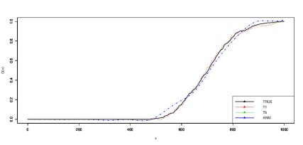
Figure 2: Estimated distribution curve for the data set of 445 students from true data set and obfuscated data-sets using Additive Noise Model and our method

Table 8: Estimates of different Statistics from original and obfuscated data-sets corresponding to 445 students

Statistic	Original	T1	Tb	ANM
”0.1”	580.8	577	574.716	543.663
”0.2”	612.8	617	613.072	604.883
”0.3”	645.2	645	643.845	654.71
”0.4”	675.6	673	671.655	684.003
”0.5”	700	699	698.033	709.56
”0.6”	727	720	724.572	736.245
”0.7”	750	750	753.56	765.846
”0.8”	786	782	789.721	798.864
”0.9”	826.6	850	850.935	836.601
”Mean”	703.047	706.189	706.189	701.878
”s.d.”	97.951	97.048	97.048	71.094
”Cor”	0.68	0.603	0.603	0.828

We can see that the process works well for real-data also.

5 Conclusion

This way of masking numerical data with a random method can be useful in various applications because it retains much of quantile and moment information even after obfuscating a data-set sufficiently, with not a huge loss in its correlation information with other non-sensitive variables. However, even if there are more than one sensitive variables, the Bernoulli variable should be chosen only once; if not, the correlation between the two sensitive variables may be hard to get back from the obfuscated data-set. If multiple sensitive attributes are present in a data-set, and some or few of them are obfuscated with this method, then studying correlation between the obfuscated variables can be an interesting problem for future work.

In our previous work, we had used Laplace Error to obfuscate the variables, but here we use Normal Error because lemma 6.1 would not hold for Laplace Error and it would become hard to get back the quantiles. Infact, any other Error distribution other than Normal may make it very hard to get back the quantiles.

Even after getting unbiased estimation for the distribution curve, the problem of performing a statistical hypothesis testing or getting a confidence interval is still a problem of concern because, even here, the variance is not easily estimable.

However, the estimation process works good for this method and gives very good estimates for large sample sizes.

6 Appendix

6.1 Proof of Theorem 2.1

Proof.

To find the raw moments of $X$, denoted by $\mu_{(X,k)}$, in terms of moments of $Z$, we first need to check that the moments of $Z$ exists whenever that of $X$ does. $k^{th}$ absolute raw moment of $Z_{i}$ is given by

$\begin{array}[]{ll}E[|Z_{i}^{k}|]&=E[|Z_{i}|^{k}\>\lvert\>B_{i}=1]\cdot P[B_{i}=1]+E[|Z_{i}|^{k}\>\lvert\>B_{i}=0]\cdot P[B_{i}=0]\\ &=p\cdot\frac{1}{n-1}\sum_{j=1,j\neq i}^{n}E[|X_{j}|^{k}\>\lvert\>j\mbox{ is chosen}]+(1-p)\cdot E[|X_{i}+Y_{i}|^{k}]\\ &=p\cdot\frac{1}{n-1}\sum_{j=1,j\neq i}^{n}{E[|X_{j}|^{k}]}+(1-p)\cdot E[|X_{i}+Y_{i}|^{k}]\\ &\leq p\cdot{E[|X_{1}|^{k}]}+(1-p)\cdot E[|X_{1}|^{k}+|Y_{1}|^{k}],\\ &\mbox{ [by Minkowski's Inequality and the fact that $X_{i}$ and $Y_{i}$'s are i.i.d.]}\\ &<\infty\end{array}$

since, $E|X_{j}|^{k}<\infty$, and $E|Y_{j}|^{k}=\frac{\sigma^{k}2^{\frac{k}{2}}\Gamma(\frac{k+1}{2})}{\sqrt{\pi}}<\infty$ $\forall k\in\mathbb{N}$.

Thus, the moments of $Z$ exists if that of $X$ exists. Now, we try to find the estimates of moments of $X$ in terms of moments of $Z$.

$\begin{array}[]{ll}\mu_{(Z,k)}&=E[Z_{i}^{k}]\\ &=E[Z_{i}^{k}\>\lvert\>B_{i}=1]\cdot P[B_{i}=1]+E[Z_{i}^{k}\>\lvert\>B_{i}=0]\cdot P[B_{i}=0]\\ &=p\cdot\frac{1}{n-1}\sum\limits_{j=1,j\neq i}^{n}{E[X_{j}^{k}]}+(1-p)\cdot E[(X_{i}+Y_{i})^{k}]\\ &=E[X_{i}^{k}]+(1-p)\{k.E[X_{i}^{k-1}]\cdot E[Y_{i}]+\ldots+E[Y_{i}^{k}]\}\\ &=\mu_{(X,k)}+(1-p)\cdot\sum\limits_{\begin{subarray}{c}j=2\\ j\mbox{ \scriptsize is even }\end{subarray}}^{2[\frac{k}{2}]}{{k\choose j}\mu_{(X,k-j)}\mu_{(Y,j)}}\end{array}$

The above equation follows since odd order moment of $Y_{i}$ is zero.

$\therefore\mu_{(X,k)}=\mu_{(Z,k)}-(1-p)\cdot\sum\limits_{j=1}^{[\frac{k}{2}]}{{k\choose 2j}{\mu_{(X,k-2j)}\mu_{(Y,2j)}}}$.

Now, $E[Z]=p\cdot E[X]+(1-p)\cdot E[X+Y]=E[X]$. $\therefore E[\frac{1}{n}\sum_{j=1}^{n}{Z_{j}}]=E[Z]=E[X]$.

$\therefore\frac{1}{n}\sum_{j=1}^{n}{Z_{j}}$ is an unbiased estimator of $E[X]$.

Define, in general,

$$\hat{\mu}_{(X,k)}=\frac{1}{n}\sum_{j=1}^{n}{Z_{j}^{k}}-(1-p)\cdot\sum\limits_{j=1}^{[\frac{k}{2}]}{{k\choose 2j}\mu_{(X,k-2j)}\mu_{(Y,2j)}}\mbox{ , $\mu_{(Y,2j)}=\sigma^{2j}\frac{2^{j}\Gamma(j+\frac{1}{2})}{\sqrt{\pi}}<\infty$}$$

If $E[\hat{\mu}_{(X,j)}]=\mu_{(X,j)}$ , $\forall j=1,2,\ldots k$ then,

$$E[\hat{\mu}_{(X,k+1)}]={\mu}_{(Z,k+1)}-(1-p)\cdot\sum_{j=1}^{[\frac{k}{2}]}{\mu_{(X,k-2j)}\mu_{(Y,2j)}}={\mu}_{(X,k+1)}$$

Thus, by induction, $\hat{\mu}_{(X,k)}$ is an unbiased estimator for ${\mu}_{(X,k)}$.

Also, note that $\hat{\mu}_{(X,k)}=\frac{1}{n}\sum_{j=1}^{n}{f(Z_{j})}$ , where $f(.)$ is a polynomial function of finite degree. Also $Var(Z_{j})=E(Z^{2j})-E(Z_{j})^{2}<\infty$ if the moments of $X$ and hence $Z$ exist and is finite $\forall n\in\mathbb{N}$. Thus $Var(\hat{\mu}_{(X,k)})=O(\frac{1}{n})$ and $\hat{\mu}_{(X,k)}$ is also a consistent estimator of $\mu_{(X,k)}$. ∎

Now, we state and prove the following lemma, which we will require while proving Theorem 2.2 and 2.3 in subsequent sections.

Lemma 6.1.

For $(x_{1},x_{2},x_{3})\in\mathbb{R}^{3}$ and $(\sigma_{1},\sigma_{2})\in\mathbb{R^{+}}^{2}$,

$$\int_{-\infty}^{\infty}{\phi_{\sigma_{1}}{(x_{1}-x_{2})}\cdot\phi_{\sigma_{2}}{(x_{2}-x_{3})}dx_{2}}=\phi_{\sqrt{\sigma_{1}^{2}+\sigma_{2}^{2}}}{(x_{1}-x_{3})}$$

where $\phi_{\sigma}(x)=$ normal density at $x\in\mathbb{R}$ for mean $0$ and standard deviation $\sigma$.

Proof.

To prove the given lemma we consider,

$\begin{array}[]{ll}L.H.S.&=\frac{1}{2\pi\sigma_{1}\sigma_{2}}\cdot\int_{-\infty}^{\infty}{e^{{-}\frac{1}{2}\cdot[(\frac{x_{1}-x_{2}}{\sigma_{1}})^{2}+(\frac{x_{2}-x_{2}}{\sigma_{2}})^{2}]}dx_{2}}\\ &=\frac{1}{2\pi\sigma_{1}\sigma_{2}}\cdot\int_{-\infty}^{\infty}{e^{{-}\frac{1}{2}\cdot[x_{2}^{2}(\frac{1}{\sigma_{1}^{2}}+\frac{1}{\sigma_{2}^{2}})-2x_{2}(\frac{x_{1}}{\sigma_{1}^{2}}+\frac{x_{3}}{\sigma_{2}^{2}})+\frac{x_{1}^{2}}{\sigma_{1}^{2}}+\frac{x_{3}^{2}}{\sigma_{2}^{2}}]}dx_{2}}\\ &=\frac{1}{\sqrt{2\pi}\sqrt{\sigma_{1}^{2}+\sigma_{2}^{2}}}\cdot e^{{-}\frac{1}{2(\frac{1}{\sigma_{1}^{2}}+\frac{1}{\sigma_{2}^{2}})}[(\frac{x_{1}}{\sigma_{1}^{2}}+\frac{x_{3}}{\sigma_{2}^{2}})^{2}-(\frac{x_{1}}{\sigma_{1}^{2}}+\frac{x_{3}}{\sigma_{2}^{2}})\cdot(\frac{1}{\sigma_{1}^{2}}+\frac{1}{\sigma_{2}^{2}})]}\\ &\hskip 71.13188pt\cdot\int_{-\infty}^{\infty}{\phi_{\frac{1}{\frac{1}{\sigma_{1}^{2}}+\frac{1}{\sigma_{2}^{2}}}}(x_{2}-(\frac{\frac{x_{1}}{\sigma_{1}^{2}}+\frac{x_{3}}{\sigma_{2}^{2}}}{\frac{1}{\sigma_{1}^{2}}+\frac{1}{\sigma_{2}^{2}}}))dx_{2}}\\ &=\frac{1}{\sqrt{2\pi}\sqrt{\sigma_{1}^{2}+\sigma_{2}^{2}}}\cdot e^{-\frac{(x_{1}-x_{3})^{2}}{2(\sigma_{1}^{2}+\sigma_{2}^{2})}}\\ &=R.H.S.\end{array}$

∎

6.2 Proof of Theorem 2.2

Proof.

Let $H(.)$ be the c.d.f. of $Z$. Then,
$\begin{array}[]{ll}H(x)&=P[Z_{i}\leq x]\\ &=P[Z_{i}\leq x\>\lvert\>B_{i}=1]\cdot P[B_{i}=1]+P[Z_{i}\leq x\>\lvert\>B_{i}=0]\cdot P[B_{i}=0]\\ &=p\cdot G(x)+(1-p)\cdot\int_{-\infty}^{\infty}{\phi_{\sigma}(x-y)G(y)dy}\\ \end{array}$
If $\tilde{G}(x)=p\cdot G(x)$, then we have the equation,

$$\tilde{G}(x)=H(x)+\lambda\int_{-\infty}^{\infty}{\phi_{\sigma}(x-y)\tilde{G}(y)dy}$$ (4)

To find a solution to Equation (4), note that this is a Fredholm Equation of second kind and a solution for such a problem for $|\lambda|<1$ is given by the famous Liouville-Neumann Series,

$$\tilde{G}(x)=\underset{n\rightarrow\infty}{lim}\sum_{t=0}^{n}{\lambda^{t}u_{t}(x)}\mbox{ , where, $u_{o}(x)=H(x)$ ,}$$ (5)

$u_{t}(x)=\int_{-\infty}^{\infty}\ldots\int_{-\infty}^{\infty}{\phi_{\sigma}(x-x_{1})\cdot\phi_{\sigma}(x_{2}-x_{1})\cdots\phi_{\sigma}(x_{t-1}-x_{t})H(x_{t})dx_{1}dx_{2}\ldots dx_{t}}$

Now $H(x)$ is unknown, so we use $\hat{H}(x)=\frac{1}{n}\sum_{j=1}^{n}{\mathbb{I}_{[Z_{j}\leq x]}}$ instead. Here, $\mathbb{I}_{A}$ is the indicator function for event $A$.
For $t\in\mathbb{N}$, the integrand in $\hat{u}_{t}(x)$ is integrable since,
$\begin{array}[]{ll}|\hat{u}_{t}(x)|&=|\int_{-\infty}^{\infty}\ldots\int_{-\infty}^{\infty}{\phi_{\sigma}(x-x_{1})\cdot\phi_{\sigma}(x_{2}-x_{1})\cdots\phi_{\sigma}(x_{t-1}-x_{t})\hat{H}(x_{t})dx_{1}dx_{2}\ldots dx_{t}}|\\ &\leq\int_{-\infty}^{\infty}\ldots\int_{-\infty}^{\infty}|{\phi_{\sigma}(x-x_{1})\cdot\phi_{\sigma}(x_{2}-x_{1})\cdots\phi_{\sigma}(x_{t-1}-x_{t})\hat{H}(x_{t})|dx_{1}dx_{2}\ldots dx_{t}}\\ &\leq\int_{-\infty}^{\infty}\ldots\int_{-\infty}^{\infty}{\phi_{\sigma}(x-x_{1})\cdot\phi_{\sigma}(x_{2}-x_{1})\cdots\phi_{\sigma}(x_{t-1}-x_{t})dx_{1}dx_{2}\ldots dx_{t}}\\ &=\int_{-\infty}^{\infty}{\phi_{\sigma\sqrt{t}}(x-x_{t})dx_{t}}\mbox{ , by lemma 5.1}\\ &=1<\infty\mbox{ , $\forall x\in\mathbb{R}$}\end{array}$
Also,

$\begin{array}[]{ll}\hat{u}_{t}(x)&=\int_{-\infty}^{\infty}\ldots\int_{-\infty}^{\infty}{\phi_{\sigma}(x-x_{1})\cdot\phi_{\sigma}(x_{2}-x_{1})\cdots\phi_{\sigma}(x_{t-1}-x_{t})\hat{H}(x_{t})dx_{1}dx_{2}\ldots dx_{t}}\\ &=\int_{-\infty}^{\infty}{\phi_{\sigma\sqrt{t}}(x-x_{t})\hat{H}(x_{t})dx_{t}}\mbox{ , by lemma 5.1}\\ &=\frac{1}{n}\sum_{j=1}^{n}{\int_{Z_{j}}^{\infty}{\phi_{\sigma\sqrt{t}}(x-x_{t})dx_{t}}}\\ &=\frac{1}{n}\sum_{j=1}^{n}{\int_{-\infty}^{x-Z_{j}}{\phi_{\sigma\sqrt{t}}(y)dy}}\mbox{ , Taking $y=x-x_{t}$}\\ &=\frac{1}{n}\sum_{j=1}^{n}{\Phi_{\sigma\sqrt{t}}(x-Z_{j})}\end{array}$

Thus $\hat{\tilde{G}}(x)=\sum_{t=0}^{\infty}{\lambda^{t}\hat{u}_{t}(x)}=\frac{1}{n}\sum_{j=1}^{n}{\sum_{t=0}^{\infty}{\lambda^{t}\Phi_{\sigma\sqrt{t}}(x-Z_{j})}}$ is an estimator of $\tilde{G}(x)$.

$\begin{array}[]{ll}E[\hat{\tilde{G}}(x)]&=\sum_{t=0}^{\infty}{\lambda^{t}E[\hat{u}_{t}(x)]}\\ &=\sum_{t=0}^{\infty}{\lambda^{t}E[\int_{-\infty}^{\infty}\ldots\int_{-\infty}^{\infty}{\phi_{\sigma}(x-x_{1})\cdots\phi_{\sigma}(x_{t-1}-x_{t})\hat{H}(x_{t})dx_{1}\ldots dx_{t}}]}\\ &=\sum_{t=0}^{\infty}{\lambda^{t}E[\int_{-\infty}^{\infty}{\phi_{\sigma\sqrt{t}}(x-x_{t})\hat{H}(x_{t})dx_{t}}]}\\ &=\sum_{t=0}^{\infty}{\lambda^{t}\int_{-\infty}^{\infty}{\phi_{\sigma\sqrt{t}}(x-x_{t})E[\hat{H}(x_{t})]dx_{t}}}\mbox{ , by Tonelli's Theorem}\\ &=\sum_{t=0}^{\infty}{\lambda^{t}\int_{-\infty}^{\infty}{\phi_{\sigma\sqrt{t}}(x-x_{t})H(x_{t})dx_{t}}}\\ &=\sum_{t=0}^{\infty}{\lambda^{t}\int_{-\infty}^{\infty}\ldots\int_{-\infty}^{\infty}{\phi_{\sigma}(x-x_{1})\cdots\phi_{\sigma}(x_{t-1}-x_{t})H(x_{t})dx_{1}\ldots dx_{t}}}\\ &=\tilde{G}(x)\end{array}$

Thus $\frac{\hat{G}(x)}{p}$ is an unbiased estimator for $G(x)$

∎

6.3 Proof of Theorem 2.3

Proof.

Note that in Equation (4), the integral term is a convolution of two functions and hence can be easily interchanged. Thus, taking derivatives on both sides we have,

$$\tilde{g}(x)=h(x)+\lambda\int_{-\infty}^{\infty}{\phi_{\sigma}(x-y)\tilde{g}(y)dy}$$ (6)

where $\tilde{g}(x)=\frac{d}{dx}\{\tilde{G}(x)\}=pg(x)$ and $g(x)$, $h(x)$ are density of $X$ and $Z$ respectively.

To find a solution to Equation (6), note that this is a Fredholm Equation of second kind and a solution for such a problem for $|\lambda|<1$ is given by the Liouville-Neumann Series,

$$\tilde{g}(x)=\underset{n\rightarrow\infty}{lim}\sum_{t=0}^{n}{\lambda^{t}u_{t}(x)}\mbox{ , where, $u_{o}(x)=h(x)$ ,}$$

$u_{t}(x)=\int_{-\infty}^{\infty}\ldots\int_{-\infty}^{\infty}{\phi_{\sigma}(x-x_{1})\cdot\phi_{\sigma}(x_{2}-x_{1})\cdots\phi_{\sigma}(x_{t-1}-x_{t})h(x_{t})dx_{1}dx_{2}\ldots dx_{t}}$

Now $h(x)$ is unknown, so we use $\hat{h}(x)=\frac{1}{n}\sum_{j=1}^{nb}{K(\frac{x-Z_{j}}{b})}$ instead. Here, $K(.)$ is the Gaussian Kernel function and $b$ is the bandwidth selected by Silvermans rule of thumb.
For $t\in\mathbb{N}$, the integrand in $\hat{u}_{t}(x)$ is integrable in a similar reason as in the proof of Theorem 2.1. Also,

$\begin{array}[]{ll}\hat{u}_{t}(x)&=\int_{-\infty}^{\infty}\ldots\int_{-\infty}^{\infty}{\phi_{\sigma}(x-x_{1})\cdot\phi_{\sigma}(x_{2}-x_{1})\cdots\phi_{\sigma}(x_{t-1}-x_{t})\hat{h}(x_{t})dx_{1}dx_{2}\ldots dx_{t}}\\ &=\int_{-\infty}^{\infty}{\phi_{\sigma\sqrt{t}}(x-x_{t})\hat{h}(x_{t})dx_{t}}\mbox{ , by lemma 5.1}\\ &=\frac{1}{n}\sum_{j=1}^{n}{\int_{-\infty}^{\infty}{\phi_{\sigma\sqrt{t}}(x-x_{t})\phi_{b}(x_{t}-Z_{j})dx_{t}}}\\ &=\frac{1}{n}\sum_{j=1}^{n}{\phi_{\sqrt{t\sigma^{2}+b^{2}}}(x-Z_{j})}\mbox{ , by lemma 5.1}\\ \end{array}$

Thus $\hat{\tilde{g}}(x)=\sum_{t=0}^{\infty}{\lambda^{t}\hat{u}_{t}(x)}=\frac{1}{n}\sum_{j=1}^{n}{\sum_{t=0}^{\infty}{\lambda^{t}\phi_{\sqrt{t\sigma^{2}+b^{2}}}(x-Z_{j})}}$ is an estimator of $\tilde{g}(x)$ and hence

$$\hat{G}(x)=\frac{1}{np}\sum_{j=1}^{n}{\sum_{t=0}^{\infty}{\lambda^{t}\Phi_{\sqrt{t\sigma^{2}+b^{2}}}(x-Z_{j})}}$$

is an estimator for $G(x)$.

Note that this estimator is a linear series of normal c.d.f.s each with positive variance and hence are smooth functions, which makes the function $\hat{G}(x)$, a smooth function.

∎

6.4 Proof of Theorem 2.4

Proof.

We have  $T_{i}(x)=\frac{1}{np}\sum_{j=1}^{n}{\sum_{t=0}^{\infty}{\lambda^{t}\Phi_{\sigma_{t}}(x-Z_{j})}}$ where $\sigma_{t}=\sigma\sqrt{t}$ for $T_{1}(x)$ and $\sqrt{t\sigma^{2}+b^{2}}$ for $T_{b}(x)$. Since, $\Phi_{\sigma_{t}}(x-Z_{j})\leq 1$ $\forall t\in\mathbb{N}$ and $\sum_{t=0}^{\infty}{\lambda^{t}}=p$, $\frac{1}{p}\sum_{t=0}^{\infty}{\lambda^{t}\Phi_{\sigma_{t}}(x-Z_{j})}=T_{ij}\mbox{ ( say)}\leq 1$.

$T_{i}(x)=\frac{1}{n}\sum_{j=1}^{n}{T_{ij}}$, i.e., average of $n$ i.i.d. random variables each of whose value is less than or equal to $1$. Thus,

$$Var(T_{i}(x))=\frac{1}{n}\cdot Var(T_{i1}(x))\leq\frac{1}{n}E(T_{i1}^{2})=O(\frac{1}{n})$$

Since $T_{1}(x)$ is unbiased, the last equation implies convergence in probability of $T_{1}(x)$ to its expected value $G(x)$. For the smooth estimator,

$$E(T_{b}(x))=E[\frac{1}{np}\sum_{j=1}^{n}{\sum_{t=0}^{\infty}{\lambda^{t}\cdot\Phi_{b_{t}}(x-Z_{j})}}]=\frac{1}{p}\sum_{t=0}^{\infty}{\lambda^{t}\int_{-\infty}^{\infty}{\Phi(\frac{x-z}{\sqrt{t\sigma^{2}+b^{2}}})h(z)dz}}$$

The true c.d.f. can be written as, (using Equation 4)

$\begin{array}[]{ll}G(x)&=\frac{1}{p}\sum\limits_{t=0}^{\infty}{\lambda^{t}\int_{-\infty}^{\infty}\ldots\int_{-\infty}^{\infty}{\phi_{\sigma}(x-x_{1})\cdots\phi_{\sigma}(x_{t-1}-x_{t})H(x_{t})dx_{1}\ldots dx_{t}}}\\ &=\frac{1}{p}\sum\limits_{t=0}^{\infty}{\lambda^{t}\int_{-\infty}^{\infty}{\phi_{\sqrt{t\sigma^{2}}}(x-x_{t})\cdot H(x_{t})dx_{t}}}\\ &=\frac{1}{p}\sum\limits_{t=0}^{\infty}{\lambda^{t}\int_{-\infty}^{\infty}{\Phi_{\sqrt{t\sigma^{2}}}(x-x_{t})h(x_{t})dx_{t}}}\\ &=\frac{1}{p}\sum\limits_{t=0}^{\infty}{\lambda^{t}\int_{-\infty}^{\infty}{\Phi(\frac{x-x_{t}}{\sqrt{t\sigma^{2}}})h(x_{t})dx_{t}}}\end{array}$

Since $\int_{-\infty}^{\infty}{\phi_{\sqrt{t\sigma^{2}}}(x-x_{t})\cdot H(x_{t})dx_{t}}=\int_{-\infty}^{\infty}{\Phi_{\sqrt{t\sigma^{2}}}(x-x_{t})\cdot h(x_{t})dx_{t}}$ both being c.d.f. of $Z+N(0,\sqrt{t\sigma^{2}})$.

Thus, we have an expression for the bias at point $x$, denoted by $B(x)$, as given below.

$\begin{array}[]{ll}|B(x)|&=|\frac{1}{p}\sum\limits_{t=0}^{\infty}{\lambda^{t}\int_{-\infty}^{\infty}[{{\Phi(\frac{x-z}{\sqrt{t\sigma^{2}+b^{2}}})}-\Phi(\frac{x-z}{\sqrt{t\sigma^{2}}})}h(z)]dz}|\\ &\leq\frac{1}{p}|\underbrace{\int_{-\infty}^{\infty}{\mathbb{I}(x-z)h(z)dz}-\int_{-\infty}^{\infty}{\Phi(\frac{x-z}{b})h(z)dz}|}_{\textsf{Tr}_{1}}\\ &~{}+\frac{1}{p}\underbrace{\sum_{t=1}^{\infty}{|\lambda|^{t}\int_{-\infty}^{\infty}{|{\Phi(\frac{x-z}{\sqrt{t\sigma^{2}+b^{2}}})}-\Phi(\frac{x-z}{\sqrt{t\sigma^{2}}})|}h(z)dz}}_{\textsf{Tr}_{2}}\end{array}$

$\begin{array}[]{ll}\textsf{Tr}_{1}&=|\int_{-\infty}^{\infty}{\mathbb{I}(x-z)h(z)dz}-\int_{-\infty}^{\infty}{\Phi(\frac{x-z}{b})h(z)dz}|\\ &=|H(x)-\int_{-\infty}^{\infty}{\Phi(x-z,0,b)h(z)dz}|\\ &=|H(x)-H^{\star}(x)|\end{array}$

where $H^{\star}(x)$ is the c.d.f. of $Z+N(0,b^{2})$, $Z$ is a r.v. with p.d.f. $h(.)$. As $n\rightarrow\infty$, $b\rightarrow 0$ and $N(0,b^{2})\overset{P}{\rightarrow}0$. Thus, by Slutsky’s theorem, $Z+N(0,b^{2})\Longrightarrow Z$ in distribution as $b\rightarrow 0$, or, $|H(x)-H^{\star}(x)|\rightarrow 0$ as $n\rightarrow\infty$.

For $\textsf{Tr}_{2}$, since $\Phi(\frac{x-z}{\sqrt{y}})$ is a continuous differentiable function in $y$, expanding the function by Taylor Series at $y=t\sigma^{2}$ we have $|{\Phi(\frac{x-z}{\sqrt{t\sigma^{2}+b^{2}}})}-\Phi(\frac{x-z}{\sqrt{t\sigma^{2}}})|=|(t\sigma^{2}+b^{2}-t\sigma^{2})(\phi(\frac{x-z}{\sqrt{y*}})\frac{x-z}{y*^{3/2}})|$ where $y^{*}$ is a point between $t\sigma^{2}$ and $t\sigma^{2}+b^{2}$. Also, it is easy to show that $|x\phi(x)|\leq 1$ for all $x\in\mathcal{R}$( as discussed in Note 5.1), which implies $|\phi(\frac{x-z}{\sqrt{y*}})\frac{x-z}{y*^{1/2}}|\leq 1$. Thus,

$\begin{array}[]{ll}\textsf{Tr}_{2}&=\sum_{t=1}^{\infty}{|\lambda|^{t}\int_{-\infty}^{\infty}{|{\Phi(\frac{x-z}{\sqrt{t\sigma^{2}+b^{2}}})}-\Phi(\frac{x-z}{\sqrt{t\sigma^{2}}})|}h(z)dz}\\ &\leq\sum_{t=1}^{\infty}{|\lambda|^{t}\frac{b^{2}}{t\sigma^{2}}}\\ &\leq\frac{b^{2}}{\sigma^{2}}\sum_{t=1}^{\infty}{\frac{|\lambda|^{t}}{t}}\\ &=\frac{b^{2}}{\sigma^{2}}\{-\log(1-|\lambda|)\}\mbox{ , where $0<|\lambda|<1$.}\\ &=C.b^{2}\rightarrow 0\mbox{ , as $b\rightarrow 0$ , where $C$ is a constant}\end{array}$

Thus $MSE(T_{b}(x))=Var(T_{b}(x))+Bias(x)^{2}\rightarrow 0\mbox{ , as $n\rightarrow\infty$}$. Hence, we have, $T_{b}(x)\overset{\mathbb{L}_{2}}{\longrightarrow}G(x)\mbox{ , $\forall x$ as $n\rightarrow\infty$ }$ which implies the result. ∎

Note 5.1: For $|x|\leq 1$, $\frac{1}{\sqrt{2\pi}}<1$, $e^{-x^{2}/2}\leq 1$ implies $|x\phi(x)|<1$. For $|x|>1$, since $|x\phi(x)|=|x|\phi(|x|)$, it can be written as $\frac{1}{\sqrt{2\pi}}\frac{|x|}{e^{|x|^{2}/2}}=\frac{1}{\sqrt{2\pi}}\frac{1}{\frac{1}{|x|}+\frac{|x|}{2}+\delta}\leq\frac{2}{\sqrt{2\pi}}<1$, where $\delta>0$.

6.5 Proof of Theorem 2.5

Proof.

For $1\leq i\leq n$, we have,

$$E[(Z_{i}-E(Z_{i}))^{2}(X^{\prime}_{i}-E(X^{\prime}_{i}))^{2}]$$

$$= pE[(Z_{i}-E(Z_{i}))^{2}(X^{\prime}_{i}-E(X^{\prime}_{i}))^{2}\>\lvert\>B_{i}=1]$$

$$~{}~{}~{}~{}+(1-p)E[(Z_{i}-E(Z_{i}))^{2}(X^{\prime}_{i}-E(X^{\prime}_{i}))^{2}\>\lvert\>B_{i}=0]$$

$$= pE[\frac{1}{n-1}\sum_{j=1,j\neq i}^{n}{[(X_{j}-E(X_{j}))^{2}(X^{\prime}_{i}-E(X^{\prime}_{i}))^{2}]}]$$

$$~{}~{}~{}~{}+(1-p)E[[(X_{i}+Y_{i}-E(X_{i}+Y_{i}))^{2}(X^{\prime}_{i}-E(X^{\prime}_{i}))^{2}]]$$

$$\mbox{ [$\because E[Y_{i}]=0$ and $E[Z_{i}]=E[X_{j}]$ $\forall 1\leq i,j\leq n$ as shown in Proof of Theorem 2.1 }]$$

$$= p\cdot Var(X^{\prime})\cdot Var(X)+(1-p)\cdot\{d(X,X^{\prime})+2\cdot 0+Var(Y)\cdot Var(X^{\prime})\}<\infty$$

Thus, $\hat{Cov}(Z,X^{\prime})=\frac{1}{n}\cdot\sum_{j=1}^{n}[{Z_{j}\cdot X^{\prime}_{j}}]-\bar{Z}\cdot\bar{X^{\prime}}$ exists and hence is a consistent estimator of the true covariance between $Z$ and $X^{\prime}$.

$$Cov(Z,X^{\prime}) = E(ZX^{\prime})-E(Z)\cdot E(X^{\prime})$$

$$= pE(X)\cdot E(X^{\prime})+(1-p)E((X+Y)\cdot X^{\prime})-E(Z)\cdot E(X^{\prime})$$

$$= (1-p)[E(X\cdot X^{\prime})-E(Z)\cdot E(X^{\prime})]$$

[$$\because E[Z]=E[X] E[YX^{\prime}]=E[Y]E[X^{\prime}]=0$$ and ]

$$= (1-p).Cov(X,X^{\prime})$$

Thus $\hat{Cov}(Z,X^{\prime})$ is a consistent estimator of $(1-p).Cov(X,X^{\prime})$, or $\frac{1}{1-p}\hat{Cov}(Z,X^{\prime})$ is a consistent estimator of $Cov(X,X^{\prime})$. Also, we have seen in Theorem 2.1, $Var(Z)$ exists if $Var(X)$ does. Thus $\sqrt{\hat{Var}(Z)}\overset{P}{\longrightarrow}\sqrt{Var(Z)}$ and since $Var(X^{\prime})$ exists, $\sqrt{\hat{Var}(X^{\prime})}\overset{P}{\longrightarrow}\sqrt{Var(X^{\prime})}$ Hence, by property of convergence in probability, the result follows.

∎

References

- [1] J. Steinberg L Pritzker. Some experiences with and reactions on data linkage in the united states, 1967, Bulletin of the International Statistical Institute, 786-808.
- [2] R. Bachi R. Baron. Confidentiality problems related to data banks, 1969, Bulletin of the International Statistical Institute, 43, pp. 225-241.
- [3] T. Dalenius The invasion of privacy problem and statistics production-an overview, 1974, Statistisk Tidskrzft, 213-225.A
- [4] T. Dalenius Computers and individual privacy some international implications, 1977a, Bulletin of the International Statistical Institute, 47, pp.203-211.
- [5] R.H. Mugge Issues in protecting confidentiality in national health statistics, 1983, Proceedings of the Section on Survey Research Methods, American Statistical Association, pp.592-594.
- [6] S.E. Fienberg Conflict between the needs for access to statistical information and demands for confidentiality, 1994, Journal of Official Statistics 10(2) pp.115-132.
- [7] S. Trabelsi V. Salzgeber M Bezzi G. Montagnon Data Disclosure Risk Evaluation, 2009, IEEE Xplore DOI: 10.1109/CRISIS.2009.5411979
- [8] W.A. Fuller Masking Procedures for Microdata Disclosure Limitation Journal of Official Statistics 1993 pp. 383-406
- [9] W.A. Fuller Measurement Error models. New York: John Wiley
- [10] T. Dalenius S. P. Reiss Data-Swapping: A Technique for Disclosure Control, 1982, Journal of Statistical Planning and Inference 6, 73-85.
-
[11]
R. A. Moore Controlled data Swapping Techniques for Masking Use Microdata Sets US Bureau of the Census, Statistical Research Division 1996
Available at http://www.census.gov/srd/www/byyear.html -
[12]
R. Sarathy & K. Muralidhar & R. Parsa Perturbing Non-normal Confidential Attributes: The Copula Approach Management Science, Vol. 48, No. 12 Dec. 2002 INFORMS pp. 1613-1627
Available at http://www.jstor.org/stable/822527 - [13] D. Ghatak & B. Roy Estimation of True Quantiles from Quantitative Data Obfuscated with Additive Noise Journal of Official Statistics In Press