Diophantine approximations on random fractals

Abstract.

We show that fractal percolation sets in $\mathbb{R}^{d}$ almost surely intersect every hyperplane absolutely winning (HAW) set with full Hausdorff dimension. In particular, if $E\subset\mathbb{R}^{d}$ is a realization of a fractal percolation process, then almost surely (conditioned on $E\neq\emptyset$), for every countable collection $\left(f_{i}\right)_{i\in\mathbb{N}}$ of $C^{1}$ diffeomorphisms of $\mathbb{R}^{d}$, $\dim_{H}\left(E\cap\left(\bigcap_{i\in\mathbb{N}}f_{i}\left(\text{BA}_{d}\right)\right)\right)=\dim_{H}\left(E\right)$, where $\text{BA}_{d}$ is the set of badly approximable vectors in $\mathbb{R}^{d}$. We show this by proving that $E$ almost surely contains hyperplane diffuse subsets which are Ahlfors-regular with dimensions arbitrarily close to $\dim_{H}\left(E\right)$.

We achieve this by analyzing Galton-Watson trees and showing that they almost surely contain appropriate subtrees whose projections to $\mathbb{R}^{d}$ yield the aforementioned subsets of $E$. This method allows us to obtain a more general result by projecting the Galton-Watson trees against any similarity IFS whose attractor is not contained in a single affine hyperplane. Thus our general result relates to a broader class of random fractals than fractal percolation.

1. Introduction

1.1. The set $\text{BA}_{d}$.

The field of Diophantine approximations deals with approximations of real numbers and vectors by rationals, where the idea is to keep the denominators as small as possible. A theorem by Dirichlet implies that for every $v\in\mathbb{R}^{d}$, there exist infinitely many $\left(P,q\right)\in\mathbb{Z}^{d}\times\mathbb{N}$, such that

$$\left\|v-\frac{P}{q}\right\|_{\infty}<\frac{1}{q^{1+\frac{1}{d}}}.$$

This result leads to one of the key definitions in the field - the badly approximable vectors.

Definition 1.1.

A vector $v\in\mathbb{R}^{d}$ is called badly approximable if there exists some $c>0$, s.t. for every $\left(P,q\right)\in\mathbb{Z}^{d}\times\mathbb{N}$,

$$\left\|v-\frac{P}{q}\right\|\geq\frac{c}{q^{1+\frac{1}{d}}}.$$

The set of all badly approximable vectors in $\mathbb{R}^{d}$ is denoted by $\text{BA}_{d}$.

Throughout this paper, $\left\|\cdot\right\|$ is the Euclidean norm, which is the only norm on $\mathbb{R}^{d}$ to be considered from this point forward. Given $x\in\mathbb{R}^{d}$ and $r>0$, $B_{r}\left(x\right)=\left\{y\in\mathbb{R}^{d}:\,\left\|x-y\right\|<r\right\}$, and finally, given a set $S\subseteq\mathbb{R}^{d}$, and $\varepsilon>0$, $S^{\left(\varepsilon\right)}$ is the $\varepsilon$-neighborhood of $S$ defined by $S^{\left(\varepsilon\right)}=\bigcup\limits_{x\in S}B_{\varepsilon}\left(x\right)$. Note that using any other norm in Definition 1.1 would result in an equivalent definition.

The set $\text{BA}_{d}$ is one of the most intensively investigated sets in the field of Diophantine approximations. It is well known that $\text{BA}_{d}$ has Lebesgue measure 0. On the other hand, it has Hausdorff dimension $d$, which makes it reasonable to surmise that it intersects various kinds of fractal sets. Indeed, in recent years there has been a lot of interest, and many results, about the intersection of $\text{BA}_{d}$ with fractal sets. A key result in this line of research is due to Broderick, Fishman, Kleinbock, Reich and Weiss [4], which deals with the intersection of $\text{BA}_{d}$ with a certain kind of fractals called hyperplane diffuse.

Definition 1.2.

Given $\beta>0$, a closed set $K\subseteq\mathbb{R}^{d}$ is called hyperplane $\beta$ - diffuse if the following holds:

$\exists\xi_{0}>0,\,\forall\xi\in\left(0,\,\xi_{0}\right),\,\forall x\in K,\,\forall\mathcal{L}\subset\mathbb{R}^{d}$ affine hyperplane,

$$K\cap B_{\xi}\left(x\right)\setminus\mathcal{L}^{\left(\beta\xi\right)}\neq\emptyset.$$

A set is called hyperplane diffuse if it is hyperplane $\beta$ - diffuse for some $\beta$.

This turns out to be a quite natural property for fractals and many interesting fractals are known to be hyperplane diffuse, especially when they have some self similarity. see Theorems 1.3 - 1.5 in [7] for some examples.

In [4] it was shown that if $K\subset\mathbb{R}^{d}$ is hyperplane diffuse, then $\dim_{H}\left(K\cap\text{BA}_{d}\right)>0$. Moreover, if $K$ is also Ahlfors-regular (defined below) then $\dim_{H}\left(K\cap\text{BA}_{d}\right)=\dim_{H}\left(K\right)$.

Definition 1.3.

For any $\delta>0$, a measure $\mu$ on $\mathbb{R}^{d}$ is called $\delta$-Ahlfors-regular , if $\exists c_{1},c_{2}>0$ s.t. $\forall\rho\in\left(0,1\right)$, $\forall x\in\text{supp}\left(\mu\right)$,

$$c_{1}\rho^{\delta}\leq\mu\left(B_{\rho}\left(x\right)\right)\leq c_{2}\rho^{\delta}$$

and Ahlfors-regular if it is $\delta$-Ahlfors-regular for some $\delta>0$. A set $K\subset\mathbb{R}^{d}$ is called Ahlfors-regular (resp. $\delta$-Ahlfors-regular) if there exists an Ahlfors-regular (resp. $\delta$-Ahlfors-regular) measure $\mu$ on $\mathbb{R}^{d}$ s.t. $\text{supp}\left(\mu\right)=K$.

This result became a main tool for studying intersections of $\text{BA}_{d}$ with fractals. The above statement is in fact a corollary of a more general theorem, where the set $\text{BA}_{d}$ is replaced by an arbitrary hyperplane absolute winning (HAW) set. These are sets which are winning in a certain game called the hyperplane absolute game, which we shall describe in section 3. Note that the set $\text{BA}_{d}$ is HAW [4]. Thus, the more general theorem is the following.

Theorem 1.4 ([4]).

Let $K\subset\mathbb{R}^{d}$ be hyperplane diffuse. Then there exists a constant $C>0$, s.t. $\forall S\subseteq\mathbb{R}^{d}$ HAW, $\dim_{H}\left(K\cap S\right)>C$. Moreover, if $K$ is Ahlfors-regular then $\dim_{H}\left(K\cap S\right)=\dim_{H}\left(K\right)$.

Two important properties of HAW sets are the following:

Theorem 1.5.

[4, Proposition 2.3]

1. Any countable intersection of HAW sets is HAW.

2. Any image of a HAW set under a $C^{1}$ diffeomorphism of $\mathbb{R}^{d}$ is HAW.

Theorem 1.5 implies for example that if $K\subseteq\mathbb{R}^{d}$ is hyperplane diffuse, then for every sequence $\left(f_{n}\right)_{n\in\mathbb{N}}$ of $C^{1}$ diffeomorphisms of $\mathbb{R}^{d}$, the intersection $K\cap\left(\bigcap_{i\in\mathbb{N}}f_{i}\left(\text{BA}_{d}\right)\right)$ has positive Hausdorff dimension, and if $K$ is also Ahlfors-regular then the Hausdorff dimension of the intersection is maximal, i.e., equal to $\dim_{H}\left(K\right)$.

1.2. Random fractals

In this paper we deal with a natural model of random fractals which we will refer to as Galton-Watson fractals. This model may be described as follows. Suppose we are given a finite IFS $\Phi=\left\{\varphi_{i}:\mathbb{R}^{d}\to\mathbb{R}^{d}\right\}_{i\in\Lambda}$ of contracting similarity maps with attractor $K$ (these notions will be explained in more detail in subsection 2.4. See also [9] for a good exposition of this topic). $\Phi$ defines a coding map $\gamma_{\Phi}:\Lambda^{\mathbb{N}}\to\mathbb{R}^{d}$ given by $\gamma_{\Phi}\left(i\right)=\bigcap\limits_{n=1}^{\infty}\varphi_{i_{1}}\circ...\circ\varphi_{i_{n}}\left(K\right)$$K$ is defined as the attractor which does not involve the coding map, so why is the definition circular? . Note that $\gamma_{\Phi}\left(\Lambda^{\mathbb{N}}\right)=K$. Let $W$ be a random variable taking values in the finite set $2^{\Lambda}$. We construct a Galton-Watson tree by iteratively choosing at random the children of each element of the tree as realizations of independent copies of $W$, starting from the root, namely $\emptyset$. By concatenating each child to its parent, this defines a random subset of the symbolic space $\Lambda^{\mathbb{N}}$ which we then project using $\gamma_{\Phi}$ to yield a random fractal $E\subset\mathbb{R}^{d}$ (which is contained in K). See Figure 1.1 for an illustrative example.

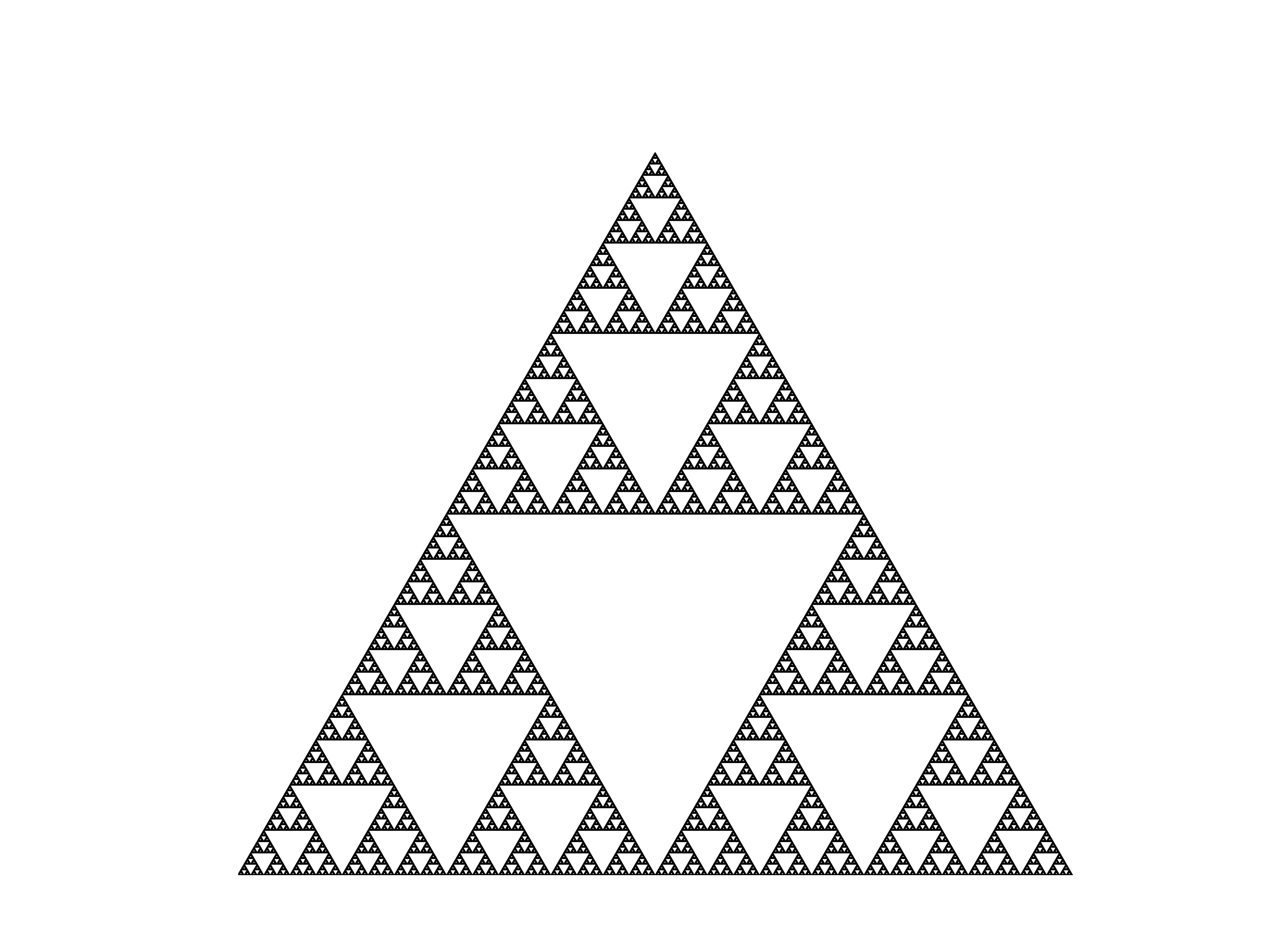
(a) The Sierpinski triangle

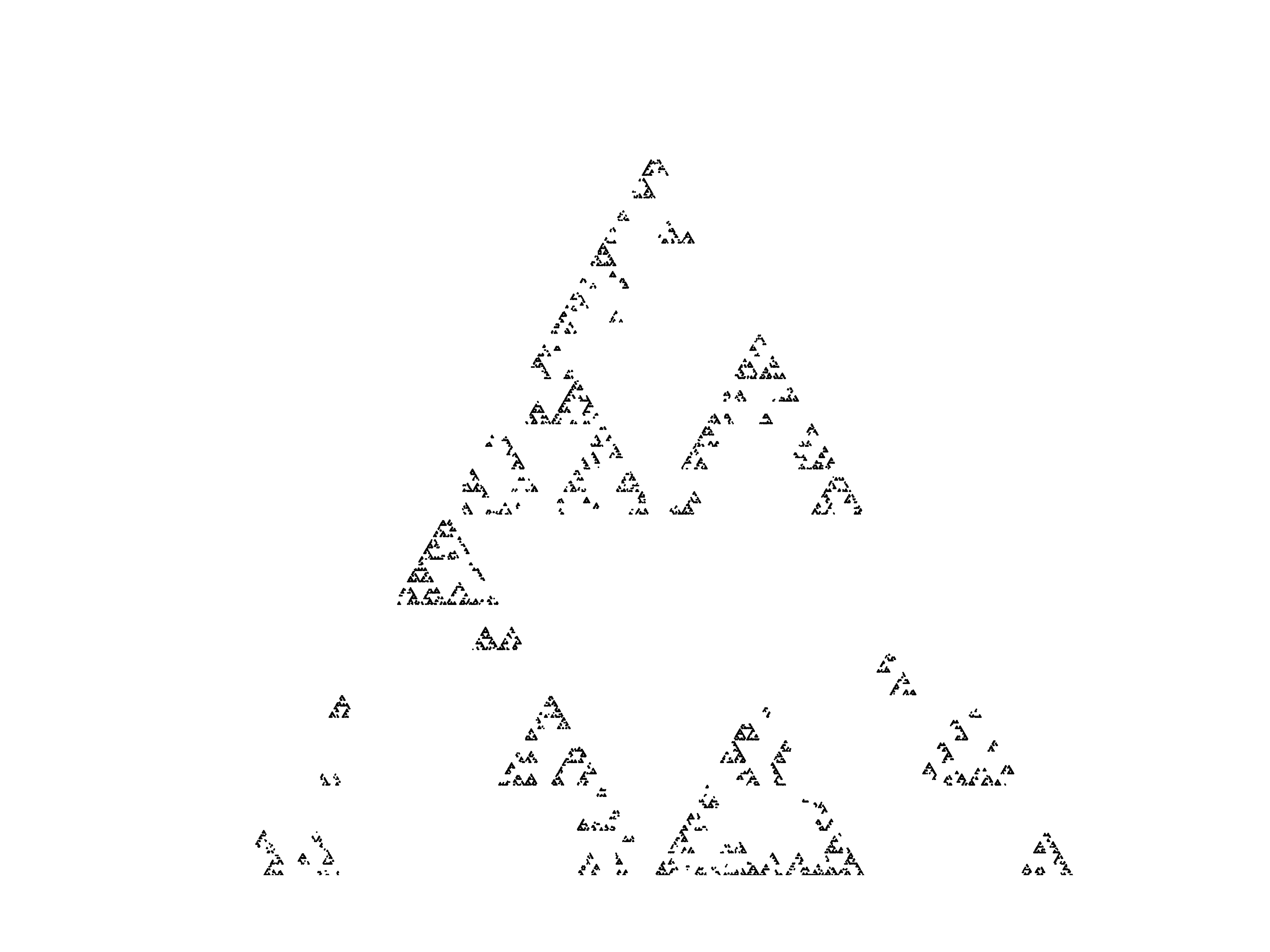
(b) The Galton-Watson fractal

Figure 1.1. An approximate realization of a Galton-Watson fractal which is constructed using an IFS whose attractor is the Sierpinski triangle, where $W$ has the distribution of a Bernoulli process on $\left\{0,1\right\}^{\Lambda}$ with parameter $p=0.8$.

Throughout the paper, we shall always assume that $\forall i\in\Lambda,\,\mathbb{P}\left(i\in W\right)>0$. Note that it is possible that at some level of the tree, no element survives and the process dies out. If this occurs we say that the process is extinct, and the resulting limit set is $E=\emptyset$. It is a well known fact that unless $\left|W\right|=1$ almost surely, $\mathbb{E}\left(\left|W\right|\right)\leq 1\iff E=\emptyset\text{ a.s.}$ (see e.g. [16, Proposition 5.1 ]). The case $\mathbb{E}\left(\left|W\right|\right)>1$ is called supercritical and we shall assume this property throughout this paper. Another well known fact is that if $\Phi$ satisfies the open set condition (abbreviated to OSC and will be defined in subsection 2.4), then a.s. conditioned on nonextinction $\dim_{H}\left(E\right)=\delta$ where $\delta$ is the unique number satisfying $\mathbb{E}\left(\sum\limits_{i\in W}r_{i}^{\delta}\right)=1$, and $r_{i}$ is the contraction ratio of $\varphi_{i}$ for each $i\in\Lambda$.

A specific example of Galton-Watson fractals that the reader should keep in mind is that of fractal percolation (AKA Mandelbrot percolation) which we now describe. Fix some $p\in[0,1]$ and some integer $b\geq 2$. Let $E_{0}\subseteq\mathbb{R}^{d}$ be the unit cube. Divide $E_{0}$ to $b^{d}$ closed subcubes of equal volume. Now, independently, retain each subcube with probability $p$ or discard it with probability $1-p$. Let $E_{1}$ be the union of all surviving subcubes. Next, for each surviving subcube in $E_{1}$ we follow the same procedure. The union of all surviving subcubes in this step will be denoted by $E_{2}$. We continue in the same fashion to produce a nested sequence $E_{0}\supseteq E_{1}\supseteq E_{2}\supseteq...$ where each set $E_{i}$ is the union of the surviving subcubes of level $i$ of the process. Eventually we take $E=\underset{i\in\mathbb{N}}{\bigcap}E_{i}$. See Figure 1.2 for an example.

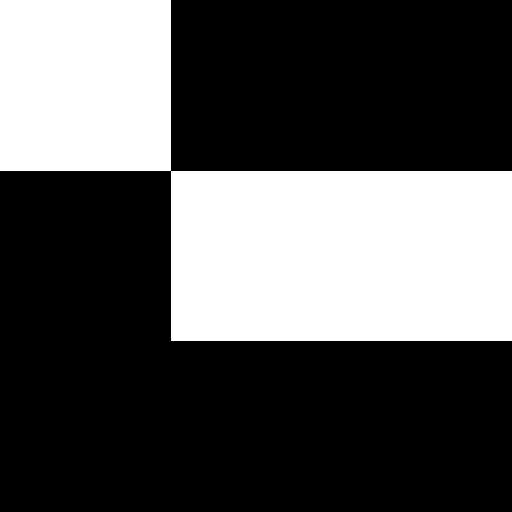
(a)

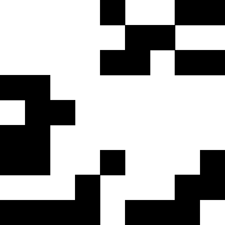
(b)

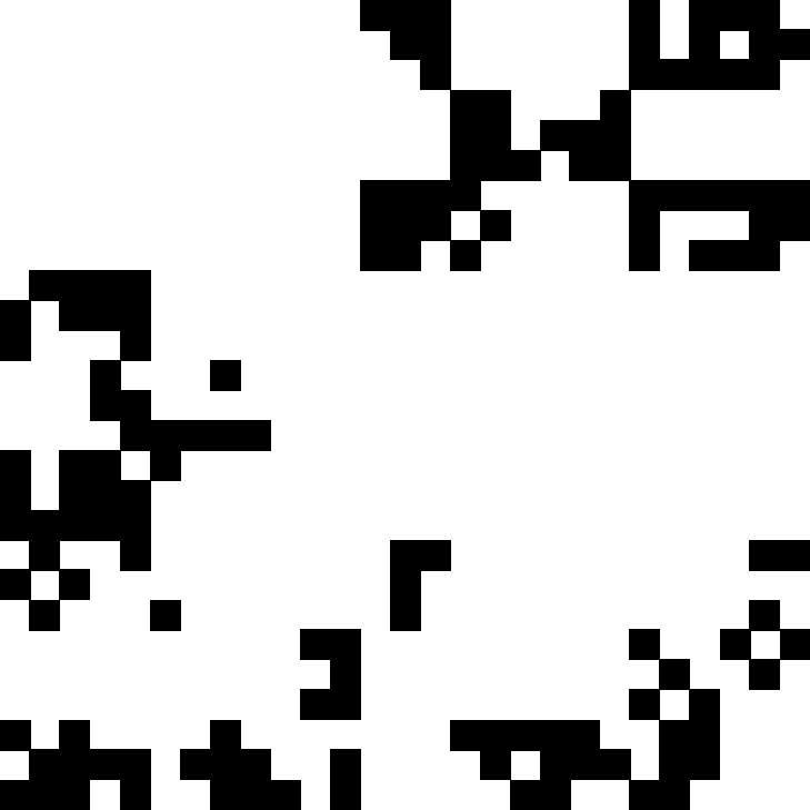
(c)

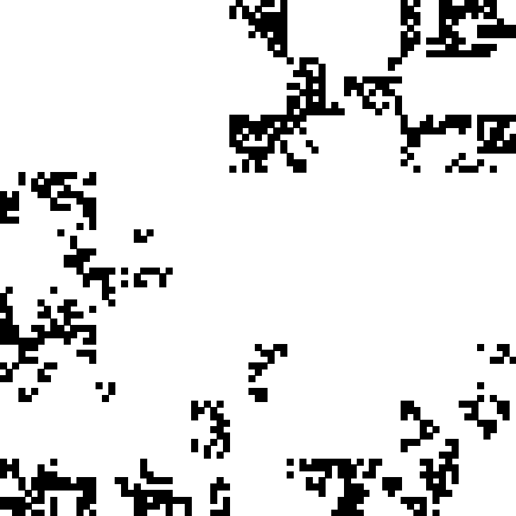
(d)

Figure 1.2. A realization of the first 4 steps of a fractal percolation process in $\mathbb{R}^{2}$ with $b=3$ and $p=0.6$.

Being a relatively simple and natural model, fractal percolation has been extensively studied over the yearsShould I add some references here? .

All the notions raised in this subsection will be defined in a more formal and detailed manner in section 2.

1.3. Main result and applications

1.3.1. Main theorem

A condition which will recur in this paper is that a Galton-Watson fractal is not a.s. contained in an affine hyperplane. Such a Galton-Watson fractal will be referred to as non-planar. Since we make the assumption that $\forall i\in\Lambda,\,\mathbb{P}\left(i\in W\right)>0$, non-planarity is essentially a property of the underlying IFS. More precisely, if $E$ is a supercritical Galton-Watson fractal w.r.t. a similarity IFS $\Phi=\left\{\varphi_{i}\right\}_{i\in\Lambda}$ and offspring distribution $W$, then $E$ is non-planar iff the attractor of $\Phi$ is not contained in an affine hyperplane. This fact as well as some other equivalent conditions to non-planarity are proved in Proposition 3.13. Note that by definition non-planar Galton-Watson fractals are supercritical.

The main theorem of this paper is the following:

Theorem 1.6.

Let E be a non-planar Galton-Watson fractal w.r.t. a similarity IFS $\Phi$. Then a.s. conditioned on nonextinction,

$$\exists C>0,\,\forall S\subset\mathbb{R}^{d}\text{ HAW, }\dim_{H}\left(E\cap S\right)>C.$$

Moreover, if in addition $\Phi$ satisfies the OSC, then a.s. conditioned on nonextinction,

$$\forall S\subset\mathbb{R}^{d}\text{ HAW, }\dim_{H}\left(E\cap S\right)=\dim_{H}\left(E\right).$$

The reader should pay special attention to the order of the quantifiers in Theorem 1.6 (a.s. $\forall S\subset\mathbb{R}^{d}$…) which is the stronger form as the collection of HAW sets is uncountable.

The proof of Theorem 1.6 is interesting mainly because in many cases (fractal percolation for example) the Galton-Watson fractal is a.s. not hyperplane diffuse (see Corollaries A.9, A.10 ). Therefore in order to prove Theorem 1.6 we prove the following:

Theorem 1.7.

Let E be a non-planar Galton-Watson fractal w.r.t. a similarity IFS $\Phi$. Then a.s. conditioned on nonextinction, $E$ contains a hyperplane diffuse subset. Moreover, if $\Phi$ satisfies the OSC, then a.s. conditioned on nonextinction, E contains a sequence of subsets $\left(D_{n}\right)_{n\in\mathbb{N}}$, s.t. for each $n\in\mathbb{N}$, $D_{n}\subseteq E$ is hyperplane diffuse and Ahlfors-regular, and $\dim_{H}\left(D_{n}\right)\nearrow\dim_{H}\left(E\right).$ Should I mention that this approach was taken before by Simmons et al?

1.3.2. Application to $\text{BA}_{d}$

Applying Theorem 1.6 to $\text{BA}_{d}$, together with Theorem 1.5, yields the following immediate corollary.

Corollary 1.8.

Let E be a non-planar Galton-Watson fractal w.r.t. a similarity IFS $\Phi$. Then a.s. conditioned on nonextinction, there exists a constant $C>0$ s.t. for every $\left(f_{i}\right)_{i\in\mathbb{N}}$ a sequence of $C^{1}$ diffeomorphisms of $\mathbb{R}^{d}$,

$$\dim_{H}\left(E\cap\left(\bigcap_{i\in\mathbb{N}}f_{i}\left(\text{BA}_{d}\right)\right)\right)>C.$$

Moreover, if in addition $\Phi$ satisfies the OSC, then a.s. conditioned on nonextinction, for every $\left(f_{i}\right)_{i\in\mathbb{N}}$ a sequence of $C^{1}$ diffeomorphisms of $\mathbb{R}^{d}$,

$$\dim_{H}\left(E\cap\left(\bigcap_{i\in\mathbb{N}}f_{i}\left(\text{BA}_{d}\right)\right)\right)=\dim_{H}\left(E\right).$$

1.3.3. Absolutely non-normal numbers and a generalization

Since Theorem 1.6 deals with any HAW set, one may consider other interesting sets which are known to be HAW. One such set is the set of absolutely non-normal numbers.

Definition 1.9.

Let $2\leq a\in\mathbb{N}$. For $x\in\mathbb{R}$, let $\left(x_{1},x_{2},...\right)$ be the digital expansion of the fractional part of $x$ in base $a$. Then $x$ is normal to base $a$ if $\forall n\in\mathbb{N},$ for every word $\omega\in\left\{0,1,...,a-1\right\}^{n}$,

$$\lim_{N\rightarrow\infty}\dfrac{1}{N}\left(\#\mbox{ occurrences of }\omega\mbox{ in }x_{1},x_{2},...,x_{N}\right)=a^{-n}$$

Following [6], $x$ will be called an absolutely non-normal number if it is normal to no base $2\leq a\in\mathbb{N}$. By ergodicity of Bernoulli shifts, the set of numbers in the unit interval which are normal to every integer base has Lebesgue measure 1. However, in [4, Theorem 2.6] following the ideas of Schmidt [22], it was shown that the set of absolutely non-normal numbers is HAW. In fact, a stronger result was proved - the set of points whose orbit under multiplication by any positive integer (mod 1) is not dense is HAW.

A generalization of this for higher dimensions is given by the following. Let $\mathbb{T}^{d}=\mathbb{R}^{d}/\mathbb{Z}^{d}$ be the $d$ - dimensional torus, and let $\pi:\mathbb{R}^{d}\rightarrow\mathbb{T}^{d}$ be the projection map. For every matrix $R\in GL_{d}\left(\mathbb{Q}\right)$ with integer entries, and every point $y\in\mathbb{T}^{d}$, we shall denote

$$\mathcal{E}\left(R,y\right)=\left\{x\in\mathbb{R}^{d}:\,y\notin\overline{\left\{\pi\left(R^{k}x\right):\,k\in\mathbb{N}\right\}}\right\}$$

Proposition 1.10.

[4, Theorem 2.6] For every nonsingular semisimple matrix with integer entries $R\in GL_{d}\left(\mathbb{Q}\right)$, and every point $y\in\mathbb{T}^{d}$, $\mathcal{E}\left(R,y\right)$ is HAW.

In particular, lifting to $\mathbb{R}^{d}$ the set of points whose orbit under $R$ is not dense in $\mathbb{T}^{d}$, yields a HAW set. A further generalization of this theorem which relates to lacunary sequences of matrices may be found in [3, Theorem 1.3].

Corollary 1.11.

Let E be a non-planar Galton-Watson fractal w.r.t. a similarity IFS $\Phi$. Then a.s. conditioned on non-extinction, $\exists C>0$ s.t. for every sequence of nonsingular semisimple matrices with integer entries $R_{i}\in GL_{d}\left(\mathbb{Q}\right)$, every sequence of points $y_{i}\in\mathbb{T}^{d}$, and every sequence $\left(f_{i}\right)_{i\in\mathbb{N}}$ of $C^{1}$ diffeomorphisms of $\mathbb{R}^{d}$,

$$\dim_{H}\left(E\cap\left(\bigcap_{i\in\mathbb{N}}f_{i}\left(\mathcal{E}\left(R_{i},y_{i}\right)\right)\right)\right)>C.$$

Moreover, if $\Phi$ satisfies the OSC, then a.s. conditioned on nonextinction, for every sequences $R_{i}$, $y_{i}$ and $f_{i}$ as above,

$$\dim_{H}\left(E\cap\left(\bigcap_{i\in\mathbb{N}}f_{i}\left(\mathcal{E}\left(R_{i},y_{i}\right)\right)\right)\right)=\dim_{H}\left(E\right).$$

Note that in the special case of $d=1$, under the above conditions, a.s. conditioned on nonextinction, the Hausdorff dimension of the absolutely non-normal numbers in $E$ is bounded from below by some positive constant, and in case $\Phi$ satisfies the OSC, this dimension is equal to $\dim_{H}\left(E\right)$.

1.4. Known results

In the special case of fractal percolation, a weaker version of Theorem 1.6 may be derived by known results. This goes through the following theorem by Hawkes [12] (see also [19, Theorem 9.5]).

Theorem 1.12.

Let E be a limit set of a supercritical fractal percolation process with parameters b,p. Let $A\subset\left[0,1\right]^{d}$ be a fixed set s.t. $\dim_{H}\left(A\right)+\log_{b}p>0$. Then

$$\text{esssup}\dim_{H}\left(A\cap E\right)=\dim_{H}A+\log_{b}p.$$

Using Hawkes’ theorem it is not hard to get the following.

Theorem 1.13.

Let E be a limit set of a supercritical fractal percolation process and let $S\subseteq\mathbb{R}^{d}$ be a HAW set. Then a.s. conditioned on non-extinction,

$$\dim_{H}\left(E\cap S\right)=\dim_{H}\left(E\right).$$

The proof of Theorem 1.13 follows immediately from Theorem 1.12 once the following general observation about HAW sets is made (see Remark 3.1): Let $S\subseteq\mathbb{R}^{d}$ be HAW, and consider the set

$$\tilde{S}=\bigcap\limits_{\left(r,q\right)\in\mathbb{Q}\times\mathbb{Q}^{d}}rS+q.$$

$\tilde{S}$ is also HAW, it is invariant under rational scaling and translations, and is contained in $S$.

The proof of Theorem 1.13 for $S$ follows from the proof for $\tilde{S}$ which is now left as an exercise for the reader.

Remark 1.14.

Note that supercritical fractal percolation processes satisfy the requirements of Theorem 1.6, i.e., the corresponding IFS satisfies the OSC, and the limit set is a.s. not contained in an affine hyperplane. Therefore, Theorem 1.6 is more general than Theorem 1.13.

Theorem 1.6 generalizes Theorem 1.13 in two aspects. First, the order of the quantifiers in Theorem 1.6 is stronger than in Theorem 1.13 and provides information about intersections of the random fractal in question with every HAW set simultaneously. Second, Theorem 1.6 allows arbitrary Galton-Watson fractals and is not restricted to fractal percolation.

1.5. Structure of the paper

The main goal of this paper is to prove Theorem 1.6. It is proved as a corollary of Theorem 1.7 which will be the focus of this paper. We first prove the theorem for the special case of fractal percolation sets as it includes most of the ideas of the proof of the general case, but is much cleaner and contains less complicated notations and definitions. This should make the ideas of the proof of the general case clearer. After that, we prove Theorem 1.7 in its full generality (the proof does not depend on the proof for fractal percolation, so the latter may be skipped).

The structure of the paper is as follows: In section 2 we define trees as subsets of a symbolic space. Then, we turn to the random setup and define Galton-Watson trees. We introduce some background and preliminary results. Then, geometry comes into play and we present the projection of trees to the Euclidean space. We introduce IFSs and the special case of fractal percolation. In section 3 we define the hyperplane absolute game and describe some related results. We then study the hyperplane diffuse property in the context of iterated function systems and Galton-Watson fractals. In section 4 we prove Theorem 1.7 for the special case of fractal percolation, and in section 5, after some required preparations, we prove the theorem in its general form. Finally, in the appendix, we provide an analysis of the microsets of Galton-Watson fractals (a notion which will be defined in Section 3) and show that in many cases (fractal percolation for example) Galton-Watson fractals are a.s. not hyperplane diffuse.

1.6. Acknowledgments

This work is a part of the author’s doctoral thesis written under the supervision of Prof. Barak Weiss. The author was partially supported by ISF grant 2095/15 and BSF grant 2016256.

2. Galton-Watson processes

2.1. Preliminaries - symbolic spaces and trees

We shall now fix some notations regarding the symbolic spaces we are about to use. Let $\mathbb{A}$ be some finite set considered as the alphabet. Denote $\mathbb{A}^{*}=\left\{\emptyset\right\}\cup\bigcup\limits_{n\in\mathbb{N}}\mathbb{A}^{n}$, this is the set of all finite words in the alphabet $\mathbb{A}$, with $\emptyset$ representing the word of length 0. Given a word $i\in\mathbb{A}^{*}$, we use subscript indexing to denote the letters comprising $i$, so that $i=i_{1}...i_{n}$ where $i_{k}\in\mathbb{A}$ for $k=1,...,n$. $\mathbb{A}^{*}$ is considered as a semigroup with the concatenation operation $\left(i_{1}...i_{n}\right)\cdot\left(j_{1}...j_{m}\right)=\left(i_{1}...i_{n},j_{1}...j_{m}\right)$ and with $\emptyset$ the identity element. The dot notation will usually be omitted so that the concatenation of two words $i,j\in\mathbb{A}^{*}$ will be denoted simply by $ij$. We will also consider the action of $\mathbb{A}^{*}$ on $\mathbb{A}^{\mathbb{N}}$ by concatenations denoted in the same way. We put a partial order on $\mathbb{A}^{*}\cup\mathbb{A}^{\mathbb{N}}$ by defining $\forall i\in\mathbb{A}^{*},\,\forall j\in\mathbb{A}^{*}\cup\mathbb{A}^{\mathbb{N}},\,i\leq j$ iff $\exists k\in\mathbb{A}^{*}\cup\mathbb{A}^{\mathbb{N}}$ with $ik=j$, that is to say $i\leq j$ iff $i$ is a prefix of $j$. Given any $i\in\mathbb{A}^{*}$ we shall denote the length of $i$ by $\left|i\right|=n$ where $n$ is the unique integer with the property $i\in\mathbb{A}^{n}$. Given any $i\in\mathbb{A}^{*}$, the corresponding cylinder set in $\mathbb{A}^{\mathbb{N}}$ is defined as $\left[i\right]=\left\{j\in\mathbb{A}^{\mathbb{N}}:\,i<j\right\}$.

Definition 2.1.

A subset $T\subseteq\mathbb{A}^{*}$ will be called a tree with alphabet $\mathbb{A}$ if $\emptyset\in T$, and for every $a\in T$, $\forall b\in\mathbb{A}^{*},\,b\leq a\implies b\in T$. We shall denote $T_{n}=T\cap\mathbb{A}^{n}$ for every $n\geq 1$, and $T_{0}=\left\{\emptyset\right\}$ so that $T=\bigcup\limits_{n\geq 0}T_{n}$. We also denote for each $a\in T$, $W_{T}\left(a\right)=\left\{i\in\mathbb{A}:\,ai\in T\right\}$. The boundary of a tree $T$ is denoted by $\partial T$ and is given by

$$\partial T=\left\{a\in\mathbb{A}^{\mathbb{N}}:\,\forall n\in\mathbb{N},\,a_{1}...a_{n}\in T_{n}\right\}.$$

The set of all trees with alphabet $\mathbb{A}$ will be denoted by $\mathscr{T}_{\mathbb{A}}\subset 2^{\mathbb{A}^{*}}$. A subtree of $T\in\mathscr{T}_{\mathbb{A}}$ is any tree $T^{\prime}\in\mathbb{\mathscr{T}_{\mathbb{A}}}$ s.t. $T^{\prime}\subseteq T$.

We continue with a few more definitions which will come in handy in what follows. Given a tree $T\in\mathscr{T}_{\mathbb{A}}$ and $a\in T$ some vertex of $T$, we denote $T^{a}=\left\{j\in\mathbb{A}^{*}:\,aj\in T\right\}\in\mathscr{T}_{\mathbb{A}}$, the descendants tree of $a$. The length of a tree $T\subseteq\mathbb{A}^{*}$ is defined by $\text{length}\left(T\right)=\sup\left\{n\in\mathbb{N}\setminus\left\{0\right\}:\,T_{n-1}\neq\emptyset\right\}$ and takes values in $\mathbb{N}\cup\left\{\infty\right\}$. A basic observation in this context is that $\forall T\in\mathscr{T}_{\mathbb{A}}$ with $\text{length}\left(T\right)=\infty$, $\partial T\neq\emptyset$.

Definition 2.2.

A finite set $\Pi\subset\mathbb{A}^{*}$ is called a section if $\bigcup\limits_{i\in\Pi}\left[i\right]=\mathbb{A}^{\mathbb{N}}$ and the union is a disjoint union. Given a tree $T\in\mathscr{T}_{\mathbb{A}}$ and a section $\Pi\subset\mathbb{A}^{*}$ we denote $T_{\Pi}=T\cap\Pi$.

Sections will play an important role in the proof of Theorem 1.7. In the fractal percolation case, it is enough to consider the sections $\mathbb{A}^{n}$ for $n\in\mathbb{N}$, therefore we postpone the discussion on sections and their intersections with random trees to subsection 5.1.

2.2. The random setup - Galton-Watson processes

Definition 2.3.

Let $\mathbb{A}$ be some finite alphabet. Let $W$ be a random variable with values in $2^{\mathbb{A}}$. Let $\left(W_{a}\right)_{a\in\mathbb{A}^{*}}$ be a (countable) collection of independent copies of $W$. We now define inductively:

• $T_{0}=\left\{\emptyset\right\}$.

• For $n\geq 1,$ $T_{n}=\bigcup\limits_{a\in T_{n-1}}\left\{aj:\,j\in W_{a}\right\}\subseteq\mathbb{A}^{n}$

If at some point $T_{n}=\emptyset$, then for every $l>n$, $T_{l}=\emptyset$ and we shall say that the process dies out or that extinction occurred. Finally we denote $T=\bigcup\limits_{n\geq 0}T_{n}$. We shall call the process $T_{0,}T_{1,}T_{2},...$ (and $T$ as well) a Galton-Watson process with alphabet $\mathbb{A}$ and offspring distribution $W$. We shall consider $T$ as a tree and refer to it as a Galton-Watson Tree (GWT). Note that $T$ is a random variable determined by the random variables $\left(W_{a}\right)_{a\in\mathbb{A}^{*}}$. As mentioned in the Introduction, we shall make the assumption that $\forall i\in\mathbb{A},\,\mathbb{P}\left(i\in W\right)>0$ (otherwise we may take a smaller alphabet without affecting the law of $T$).

By definition $\mathscr{T}_{\mathbb{A}}\subset 2^{\mathbb{A}^{*}}$. As sets, $2^{\mathbb{A}^{*}}\approx\prod\limits_{n=0}^{\infty}2^{\mathbb{A}^{n}}$ with the convention that $A^{0}=\left\{\emptyset\right\}$, thus $2^{\mathbb{A}^{*}}$ may be endowed with the product topology of $\prod\limits_{n=0}^{\infty}2^{\mathbb{A}^{n}}$ which is metrizable, separable and compact (where each $2^{\mathbb{A}^{n}}$ carries the discrete topology). With this topology, $\mathscr{T}_{\mathbb{A}}$ is a closed subset of $2^{\mathbb{A}^{*}}$, and from this point forward $\mathscr{T}_{\mathbb{A}}$ will carry the topologyThe definition of the topology is only required for the appendix. Should it be moved? induced by $2^{\mathbb{A}^{*}}$.

Given a finite tree $L\subset\mathbb{A}^{*}$, let $\left[L\right]\subset\mathscr{T}_{\mathbb{A}}$ be defined by

$$\left[L\right]=\left\{S\in\mathscr{T}_{\mathbb{A}}:\,\forall n\in\mathbb{N},\,L_{n}\neq\emptyset\implies S_{n}=L_{n}\right\}$$

These sets form a basis for the topology of $\mathscr{T}_{\mathbb{A}}$ and generate the Borel $\sigma$-algebra on $\mathscr{T}_{\mathbb{A}}$ which we denote by $\mathscr{B}$. By Kolmogorov’s extension theorem the Galton-Watson process yields a unique Borel measure on $\mathscr{T}_{\mathbb{A}}$ which we denote by $\mathscr{GW}$ and is the distribution of the random variable $T$. The careful reader will notice that all the events in this paper whose probability is analyzed are in $\mathscr{B}$. For any measurable property $\mathscr{T}^{\prime}\subseteq\mathscr{T}_{\mathbb{A}}$, the notation $\mathbb{P}\left(T\in\mathscr{T}^{\prime}\right)$ means $\mathscr{GW}\left(\mathscr{T}^{\prime}\right)$.

For each $n\geq 0$, we denote $Z_{n}=\left|T_{n}\right|$. We note that the usual definition of a Galton-Watson process (as defined e.g. in [16]) would be the random process $\left(Z_{n}\right)_{n\geq 1}$, but in our case it is important to keep track of the labels as later on we are going to project these trees to the Euclidean space (in the beginning of subsection 2.4). Nevertheless, in some cases where the labels aren’t important we shall refer to the process $\left(Z_{n}\right)_{n\geq 1}$ as a Galton-Watson process as well.

Given a Galton-Watson process, we shall denote $m=\mathbb{E}\left(Z_{1}\right)$. It is a basic fact that for every $n\geq 1$, $\mathbb{E}\left(Z_{n}\right)=m^{n}$. As mentioned in section 1, the process is called supercritical when $m>1$, in which case $\mathbb{P}\left(\text{nonextinction}\right)>0$.

The following is a basic result in the theory of Galton-Watson processes ([14], see also [16]).

Theorem 2.4 (Kesten-Stigum).

Let $\left(Z_{k}\right)_{k=1}^{\infty}$ be a supercritical Galton-Watson process, then $\dfrac{Z_{k}}{m^{k}}$ converges a.s. (as $k\to\infty$) to a random variable $L$, where $\mathbb{E}\left(L\right)=1$ and $L>0$ a.s. conditioned on nonextinction.

An immediate corollary of Theorem 2.4 is the following.

Corollary 2.5.

Let $\left(Z_{k}\right)_{k=1}^{\infty}$ be a supercritical Galton-Watson process, then the following holds.

$$\forall\varepsilon>0,\,\exists c>0,\,\exists K_{0}\in\mathbb{N},\,\forall k>K_{0},\,\mathbb{P}\left(\dfrac{Z_{k}}{m^{k}}>c\mid\,\text{nonextinction}\right)>1-\varepsilon.$$

The proof of Corollary 2.5 is standard and is left as an exercise to reader.

The following proposition is a result of the statistical self similarity of the Galton-Watson processes, that is, the fact that for every $v\in T$, the tree $T^{v}$ is itself a GWT with the same offspring distribution as $T$, and that for $v,w\in T$ which are not descendants of each other, $T^{v}$ and $T^{w}$ are independent.

Proposition 2.6.

Let $T$ be a supercritical Galton-Watson tree with alphabet $\mathbb{A}$ and let $\mathscr{T}^{\prime}\subseteq\mathscr{T}_{\mathbb{A}}$ be a measurable subset. Suppose that $\mathbb{P}\left(T\in\mathscr{T}^{\prime}\right)>0$, then a.s. conditioned on nonextinction, there exist infinitely many $v\in T$ s.t. $T^{v}\in\mathscr{T}^{\prime}$.

Proof.

By Corollary 2.5, given some $\varepsilon>0$, there exists a constant $c>0$ s.t.

$$\mathbb{P}\left(\left|T_{k}\right|>cm^{k}\mid\,\text{nonextinction}\right)>1-\varepsilon$$

whenever $k$ is large enough. Denote $\rho=\mathbb{P}\left(T\in\mathscr{T}^{\prime}\right)$. Given any $M>0$,

$$\begin{array}[]{l}\mathbb{P}\left(\left|\left\{v\in T_{k}:\,T^{v}\in\mathscr{T}^{\prime}\right\}\right|<M\mid\,\text{nonextinction},\,\left|T_{k}\right|>cm^{k}\right)\leq\\ {\displaystyle\mathbb{P}\left(\text{Bin}\left(cm^{k},\,\rho\right)<M\right)\leq}\\ \dfrac{\rho\left(1-\rho\right)cm^{k}}{\left[\rho cm^{k}-M\right]^{2}}\underset{k\rightarrow\infty}{\longrightarrow}0\end{array}$$

In the last inequality we used Chebyshev’s inequality assuming that $k$ is large enough so that $\rho cm^{k}>M$.∎

2.3. A generalization of Pakes-Dekking theorem

In this subsection we show how to prove the existence of certain subtrees in GWTs.

Definition 2.7.

Given a nonempty collection of nonempty subsets of the alphabet $\mathscr{A}\subseteq 2^{\mathbb{A}}$, a tree $T\in\mathscr{T}_{\mathbb{A}}$ is called an $\mathscr{A}$-tree if for every $a\in T$, $W_{T}\left(a\right)\in\mathscr{A}$. Note that by definition $\mathscr{A}$-trees are infinite. A finite tree $T$ will be called an $\mathscr{A}$-tree of length $n$, if $\text{length}\left(T\right)=n$ and $\forall a\in T\setminus T_{\text{length}\left(T\right)-1}$, $W_{T}\left(a\right)\in\mathscr{A}$. Given a tree $S\in\mathscr{T}_{\mathbb{A}}$, an $\mathscr{A}$-subtree (respectively, $\mathscr{A}$-subtree of length $n$) of $S$ is a subtree of $S$ which is an $\mathscr{A}$-tree (respectively, $\mathscr{A}$-tree of length $n$).

Given a collection $\mathscr{A}\subseteq 2^{\mathbb{A}}$ as above, we denote $\overline{\mathscr{A}}=\left\{S\in 2^{\mathbb{A}}:\,\exists X\in\mathscr{A},\,X\subseteq S\right\}$. It is obvious that $T$ has an $\overline{\mathscr{A}}$-subtree iff $T$ has an $\mathscr{A}$-subtree. $\mathscr{A}$ will be called monotonic if $\overline{\mathscr{A}}=\mathscr{A}$.

Lemma 2.8.

Let $T\in\mathscr{T}_{\mathbb{A}}$ be a tree with alphabet $\mathbb{A}$, and let $\mathscr{A}\subseteq 2^{\mathbb{A}}$ be some collection as above. Then $T$ has an infinite $\mathscr{A}$-subtree $\iff$ $\forall n\in\mathbb{N}$, $T$ has an $\mathscr{A}$-subtree of length $n$.

Proof.

For every $n\in\mathbb{N}$, let $S^{\left(n\right)}$ be an $\mathscr{A}$-subtree of $T$ of length $n$. Denote $S=\bigcup\limits_{n=1}^{\infty}S^{\left(n\right)}$. $S$ is a subtree of $T$, and since $\text{length}\left(S\right)=\infty$, $\partial S\neq\emptyset$. Define $S^{\prime}=\left\{v<w:\,w\in\partial S\right\}$. Then $S^{\prime}$ is an $\overline{\mathscr{A}}$-subtree of $T$, and therefore contains an $\mathscr{A}$-subtree. The other direction is trivial. ∎

The following theorem is the main tool we use to show that certain $\mathscr{A}$-subtrees exist in GWTs. This theorem is a generalization of a theorem by Pakes and Dekking ([21], see also [16]) which deals with the existence of a-ary subtrees (where each element has exactly a children) in Galton-Watson trees. First, we need the following definition.

Definition 2.9.

Let $A$ be some finite set, and $p\in\left[0,1\right]$. A random subset $Y\subseteq A$ is said to have a binomial distribution with parameter $p$ if

$$\forall B\subseteq A,\,\mathbb{P}\left(Y=B\right)=p^{\left|B\right|}\left(1-p\right)^{\left|A\setminus B\right|}.$$

In this case we denote $Y\sim\text{Bin}\left(A,\,p\right)$. Note that the notation $\text{Bin}\left(\cdot,\cdot\right)$ will also be used for the usual binomial distribution as well, where the first argument will be an integer and not a set.

The following notation will recur throughout the paper. Let $A$ be some fixed finite set, and let $X$ be a random subset of $A$. Given $s\in\left[0,1\right]$, we denote $X^{\left(s\right)}=X\cap Y$ where $Y\sim\text{Bin}\left(A,\,1-s\right)$.

Let $T$ be a GWT with alphabet $\mathbb{A}$ and any offspring distribution $W$. Let $\mathscr{A}\subseteq 2^{\mathbb{A}}$ be some nonempty collection of nonempty subsets of $\mathbb{A}$. Define the function $g_{\mathscr{A}}:\left[0,1\right]\rightarrow\left[0,1\right]$ by $g_{\mathscr{A}}\left(s\right)=\mathbb{P}\left(W^{\left(s\right)}\notin\overline{\mathscr{A}}\right)$. Finally, denote $\tau\left(\mathscr{A}\right)=\mathbb{P}\left(\text{$T$ has an $\mathscr{A}$-subtree}\right)$.

Theorem 2.10.

With notations as above, $1-\tau\left(\mathscr{A}\right)$ is the smallest fixed point of $g_{\mathscr{A}}$ in $\left[0,1\right]$.

Proof.

We follow the Proof given in [16, chapter 5] almost verbatim. Note that the following properties hold:

1. $g_{\mathscr{A}}$ is continuous and monotonically increasing.

2. $g_{\mathscr{A}}\left(1\right)=1$

3. $g_{\mathscr{A}}\left(0\right)=\mathbb{P}\left(W\notin\overline{\mathscr{A}}\right)$

If $g_{\mathscr{A}}\left(0\right)=0$, then $\mathbb{P}\left(W\in\overline{\mathscr{A}}\right)=1$ which implies the existence of an $\mathscr{A}$ - subtree a.s., i.e., $1-\tau\left(\mathscr{A}\right)=0$ and the claim follows. Otherwise, we assume that $g_{\mathscr{A}}\left(0\right)>0$. Let $q_{n}$ be the probability that $T$ does not contain an $\mathscr{A}-\text{subtree}$ of length $n$, where $q_{0}=0$. Then $1-q_{n}\searrow\mathbb{P}\left(T\text{ has an $\mathscr{A}$-subtree of every length}\right)$ and by Lemma 2.8 this is equivalent to $q_{n}\nearrow 1-\tau\left(\mathscr{A}\right)$.

Claim.

For every $n\geq 1$, $q_{n}=g_{\mathscr{A}}\left(q_{n-1}\right)$.

proof of claim.

Denote for every $n\geq 1$, the following random set:

$$V_{n}=\left\{v\in T_{1}:\,T^{v}\,\text{has an $\mathscr{A}$-subtree of length $n$}\right\}.$$

For each element $v\in\mathbb{A}$, $\mathbb{P}\left(v\in V_{n}|\,v\in T_{1}\right)=1-q_{n}$, and for every two distinct elements in $\mathbb{A}$ these events are independent, so $V_{n}\sim W^{\left(q_{n}\right)}$. Now, since $T$ has an $\mathscr{A}$-subtree of length $n$ iff $V_{n-1}\in\overline{\mathscr{A}}$,

$$q_{n}=\mathbb{P}\left(V_{n-1}\notin\overline{\mathscr{A}}\right)=\mathbb{P}\left(W^{\left(q_{n-1}\right)}\notin\overline{\mathscr{A}}\right)=g_{\mathscr{A}}\left(q_{n-1}\right).$$

∎

Since $g_{\mathscr{A}}$ is increasing and continuous, its smallest fixed point is $\lim\limits_{n\to\infty}g_{\mathscr{A}}^{n}\left(0\right)$, where $g_{\mathscr{A}}^{n}$ denotes the composition of $g_{\mathscr{A}}$ with itself $n$ times (this is a general property of increasing and continuous functions on $\left[0,1\right]$ whose proof is easy and left to the reader). By the claim above, $\lim\limits_{n\to\infty}g_{\mathscr{A}}^{n}\left(0\right)=\lim\limits_{n\to\infty}q_{n}$ which concludes the proof.

∎

Remark 2.11.

Given some integer $1\leq a\leq\left|\mathbb{A}\right|$, we may set $\mathscr{A}=\left\{S\subseteq\mathbb{A}:\,\left|S\right|=a\right\}$. In this case $\mathscr{A}$-subtrees are actually a-ary subtrees and Theorem 2.10 becomes exactly Pakes - Dekking theorem.

Combining Theorem 2.10 and Proposition 2.6 we obtain the following.

Corollary 2.12.

With notations as above, if $g_{\mathscr{A}}$ has some fixed point $<1$, then almost surely conditioned on nonextinction, there exist infinitely many $v\in T$ s.t. $T^{v}$ contains an $\mathscr{A}$-subtree.

2.4. IFSs and projections to $\mathbb{R}^{d}$

An iterated function system (IFS) is a finite collection $\left\{\varphi_{i}\right\}_{i\in\Lambda}$ of self maps of $\mathbb{R}^{d}$ which are Lipschitz continuous with Lipschitz constants smaller than 1. It is one of the most basic results in fractal theory (due to Hutchinson [13]) that every IFS $\left\{\varphi_{i}\right\}_{i\in\Lambda}$ gives rise to a unique nonempty compact set $K\subset\mathbb{R}^{d}$ which satisfies the equation $K=\bigcup\limits_{i\in\Lambda}\varphi_{i}K$. The set $K$ is called the attractor of the IFS.

A map $f:\mathbb{R}^{d}\rightarrow\mathbb{R}^{d}$ is called a contracting similarity if there exists a constant $r\in\left(0,1\right)$, referred to as the contraction ratio of $f$, s.t. $\forall x,y\in\mathbb{R}^{d},\,\left\|f\left(x\right)-f\left(y\right)\right\|=r\left\|x-y\right\|$, so that $f$ is a composition of a scaling by factor $r$, an orthogonal transformation and a translation. In this paper we shall only discuss IFSs which are formed by contracting similarity maps. Such IFSs shall be referred to as similarity IFSs.

When analyzing a similarity IFS $\Phi=\left\{\varphi_{i}\right\}_{i\in\Lambda}$ it is natural to work in the symbolic spaces $\Lambda^{\mathbb{N}}$ and $\Lambda^{*}$. In view of the setup above, in the abstract setting of trees with alphabet $\mathbb{A}$, we shall often assign weights to the alphabet $\left\{r_{i}\right\}_{i\in\mathbb{A}}$. These weights will correspond to the contraction ratios of similarity maps and therefore we shall always assume that $r_{i}\in\left(0,1\right)$ for every $i\in\mathbb{A}$.

Given an IFS $\left\{\varphi_{i}\right\}_{i\in\Lambda}$, the identification between the symbolic spaces $\Lambda^{\mathbb{N}},\,\Lambda^{*}$ and the Euclidean space is made via the coding map $\gamma_{\Phi}:\Lambda^{\mathbb{N}}\rightarrow\mathbb{R}^{d}$ which is given by

(2.1) $$\gamma_{\Phi}\left(j\right)=\bigcap\limits_{n=1}^{\infty}\varphi_{j_{1}...j_{n}}\left(K\right)$$

where $\varphi_{j_{1}...j_{n}}=\varphi_{j_{1}}\circ...\circ\varphi_{j_{n}}$. It may be easily seen that $K=\gamma_{\Phi}\left(\Lambda^{\mathbb{N}}\right)$. Moreover, given a tree $T\in\Lambda^{*}$, we may project the boundary of $T$ to the Euclidean space using $\gamma_{\Phi}$, where

(2.2) $$\gamma_{\Phi}\left(\partial T\right)=\bigcup_{j\in\partial T}\bigcap\limits_{n=1}^{\infty}\varphi_{j_{1}...j_{n}}\left(K\right)=\bigcap\limits_{n=1}^{\infty}\bigcup\limits_{i\in T_{n}}\varphi_{i}K$$

Note that for every compact set $F\subset\mathbb{R}^{d}$ s.t. $\forall i\in\Lambda,\,\varphi_{i}F\subseteq F$, we have $K=\bigcap\limits_{n=1}^{\infty}\bigcup\limits_{i\in\Lambda^{n}}\varphi_{i}F$, hence $K\subseteq F$ and the decreasing sequence of sets $\left(\bigcup\limits_{i\in\Lambda^{n}}\varphi_{i}F\right)_{n=1}^{\infty}$ may be thought of as approximating $K$. Since $K\subseteq F$, we may replace $K$ with $F$ in equations (2.1), (2.2) and the equations will remain true.

An IFS $\left\{\varphi_{i}\right\}_{i\in\Lambda}$ satisfies the open set condition (OSC) if there exists some nonempty open set $U\subset\mathbb{R}^{d}$ s.t. $\varphi_{i}U\subseteq U$ for every $i\in\Lambda$, and $\varphi_{i}U\cap\varphi_{j}U=\emptyset$ for distinct $i,\,j\in\Lambda$. A set U satisfying these conditions will be called an OSC set for $\Phi$. In case an IFS $\Phi=\left\{\varphi_{i}\right\}_{i\in\Lambda}$ with contraction ratios $\left\{r_{i}\right\}_{i\in\Lambda}$ satisfies the open set condition, it is well known that the Hausdorff dimension of the attractor of $\Phi$ is the unique number $\delta$ which satisfies the equation $\sum\limits_{i\in\Lambda}r_{i}^{\delta}=1$ . For convenience, $\forall i=i_{1}...i_{n}\in\Lambda^{*}$ we denote $r_{i}=r_{i_{1}}\cdots r_{i_{n}}$ which is the contraction ratio of the map $\varphi_{i}$. We also denote $r_{min}=\min\left\{r_{i}:\,i\in\Lambda\right\}$ and $r_{max}=\max\left\{r_{i}:\,i\in\Lambda\right\}$.

We shall now turn to the probabilistic setup.

Definition 2.13.

Let $\Phi=\left\{\varphi_{i}\right\}_{i\in\Lambda}$ be a similarity IFS, and let $W$ be some random variable with values in $2^{\Lambda}$. Let $T$ be a GWT with alphabet $\Lambda$ and offspring distribution $W$, and finally let $E$ be the random set $E=\gamma_{\Phi}\left(\partial T\right)$. The random set $E$ will be called a Galton-Watson fractal (GWF) w.r.t. the IFS $\Phi$ and offspring distribution $W$. We shall always assume that $\mathbb{E}\left(\left|W\right|\right)>1$ so that the Galton-Watson process is supercritical.

The following theorem is due to Falconer [8] and Mauldin and Williams [17]. See also [16, Theorem 15.10] for another elegant proof.

Theorem 2.14.

Let E be a Galton-Watson fractal w.r.t. a similarity IFS $\Phi=\left\{\varphi_{i}\right\}_{i\in\Lambda}$ satisfying the OSC, with contraction ratios $\left\{r_{i}\right\}_{i\in\Lambda}$ and offspring distribution W. Then a.s. conditioned on nonextinction, $\dim_{H}E=\delta$ where $\delta$ is the unique number satisfying

$$\mathbb{E}\left(\sum_{i\in W}r_{i}^{\delta}\right)=1.$$

2.5. Fractal percolation

Fractal percolation is an important special case of GWFs. In general, it is easier to analyze since it has more independence, the maps of the corresponding IFS have a trivial orthogonal component (i.e. they are only composed of scaling and translation transformations), and all the contraction ratios are equal. In our case, it is mainly the last property which makes things less complicated.

To describe fractal percolation in the framework defined above, fix an integer $b\geq 2$ and $p\in\left(0,1\right)$. Denote $\Lambda_{b}=\left\{0,\,1,\,...,\,b-1\right\}^{d}$ (since in this section $b$ is fixed we will not carry the subscript $b$ and just write $\Lambda$ instead of $\Lambda_{b}$). Construct a GWT with alphabet $\Lambda$ and binomial offspring distribution, i.e., $W\sim\text{Bin}\left(\Lambda,\,p\right)$.

The coding map is the $b$-adic coding map $\gamma_{b}:\Lambda^{\mathbb{N}}\rightarrow\left[0,1\right]^{d}$ given by

$$\gamma_{b}\left(i\right)=\sum\limits_{k=1}^{\infty}b^{-k}i_{k},\,\,\,\forall i\in\Lambda^{\mathbb{N}}.$$

Note that each $i_{k}$ in the above formula is a vector in $\mathbb{R}^{d}$.

This coding map corresponds to the similarity IFS consisted of the homotheties mapping the unit cube to each $b$-adic cube, i.e., $\varphi_{i}\left(x\right)=\frac{1}{b}\cdot x+\frac{i}{b}$ for every $i\in\Lambda,\,x\in\mathbb{R}^{d}$. Note that there is a correspondence between elements of $\Lambda^{n}$ and closed b-adic subcubes of the $n^{th}$ level, where for each element $j\in\Lambda^{n}$ the corresponding closed b-adic cube is given by $\gamma\left(\left[j\right]\right)$.

Set for each $n$, $E_{n}=\bigcup\limits_{j\in T_{n}}\gamma\left(\left[j\right]\right)$, then the limit set $E$ is given by

$$E=\bigcap_{n\in\mathbb{N}}E_{n}=\gamma_{b}\left(\partial T\right).$$

Note that in the supercritical case, by Theorem 2.14, a.s. conditioned on nonextinction,

$$\dim_{H}E=\log_{b}\left(m\right).$$

Recall that $m=\mathbb{E}\left(Z_{1}\right)$, and in case of fractal percolation in $\mathbb{R}^{d}$ with parameters $b,p$, $m=pb^{d}$.

3. Hyperplane diffuse sets

3.1. The hyperplane absolute game

The hyperplane absolute game, developed in [4], is a useful variant of Schmidt’s game which was invented by W. Schmidt in [22] and became a main tool for the study of $\text{BA}_{d}$.

The hyperplane absolute game is played between two players, Bob and Alice and has one fixed parameter $\beta\in\left(0,\frac{1}{3}\right)$. Bob starts by defining a closed ball $B_{1}=B_{\rho_{1}}\left(x_{1}\right)\subset\mathbb{R}^{d}$. Then, for every $i\in\mathbb{N}$, after Bob has chosen a ball $B_{i}=B_{\rho_{i}}\left(x_{i}\right)$, Alice chooses an affine hyperplane $\mathcal{L}_{i}\subset\mathbb{R}^{d}$ and an $\varepsilon_{i}\in\left(0,\beta\rho_{i}\right)$, and removes the $\varepsilon_{i}$-neighborhood of $\mathcal{L}_{i}$ denoted by $A_{i}=\mathcal{L}_{i}^{\left(\varepsilon_{i}\right)}$ from $B_{i}$. Then Bob chooses his next ball $B_{i+1}=B_{\rho_{i+1}}\left(x_{i+1}\right)\subset B_{i}\setminus A_{i}$ with the restriction on the radius $\rho_{i+1}\geq\beta\rho_{i}$. The game continues ad infinitum. A set $S\subset\mathbb{R}^{d}$ is called hyperplane absolute winning (HAW) if for every $\beta\in\left(0,\frac{1}{3}\right)$, Alice has a strategy guaranteeing that $\bigcap\limits_{n=1}^{\infty}B_{n}$ intersects $S$. Note that existence of such a strategy for some $\beta\in\left(0,\frac{1}{3}\right)$, implies the existence of a strategy for every $\beta^{\prime}\in\left(\beta,\frac{1}{3}\right)$.

Many interesting sets are known to be HAW (see e.g. [1, 10, 20]), including the set $\text{BA}_{d}$ [4, Theorem 2.5]. Note that HAW sets in $\mathbb{R}^{d}$ are always dense and have Hausdorff dimension $d$. Also, as stated in Theorem 1.5, the HAW property is preserved under countable intersections and $C^{1}$ diffeomorphisms, which make these sets “large”. The following observation may be found useful.

Remark 3.1.

Let $S\subseteq\mathbb{R}^{d}$ be HAW. Then for every countable group $G$ of $C^{1}$ diffeomorphisms of $\mathbb{R}^{d}$, $S$ contains a $G$ - invariant set $\tilde{S}$ which is also HAW. Indeed, we may take $\tilde{S}=\bigcap\limits_{g\in G}gS$, and by Theorem 1.5, $\tilde{S}$ is itself HAW. This property may be useful in some cases, and as an example we already saw a use for this property in Theorem 1.13.

Although HAW sets are “large” in the senses mentioned above, as in the case of $\text{BA}_{d}$, HAW sets may have Lebesgue measure 0.

A key feature of HAW sets is given in Theorem 1.4, which states, generally speaking, that HAW sets intersect hyperplane diffuse sets. While the definition of the hyperplane diffuse property given in the Introduction (Definition 1.2) may seem a bit technical and maybe tailored for the hyperplane absolute game, an equivalent definition of this property using the notion of microsets (which was coined by H. Furstenberg in [11]) indicates that it is actually quite natural.

Definition 3.2.

Given a compact set $C\subset\mathbb{R}^{d}$, we denote

$$\Omega_{C}=\left\{A\subseteq C:\,A\text{ is compact and nonempty}\right\}.$$

We equip $\Omega_{C}$ with the Hausdorff metric which we denote by $d_{H}$, and is given by

$$\forall A,B\in\Omega_{C},\,d_{H}\left(A,B\right)=\inf\left\{\varepsilon>0:\,A\subseteq B^{\left(\varepsilon\right)}\,\wedge\,B\subseteq A^{\left(\varepsilon\right)}\right\}.$$

It is a well known fact that as a metric space $\left(\Omega_{C},d_{H}\right)$ is compact.

Given a (closed or open) ball with radius $r>0$ and center point $x\in\mathbb{R}^{d}$, we define $F_{B}:\mathbb{R}^{d}\rightarrow\mathbb{R}^{d}$ by $F_{B}\left(t\right)=\frac{1}{r}\left(t-x\right)$, so that $F_{B}$ is the unique homothety mapping $B$ to the unit ball.

Definition 3.3.

Let $K\subseteq\mathbb{R}^{d}$ be a compact set. A set of the form $F_{B}\left(K\cap B\right)$ where $B$ is a closed ball centered in $K$ is called a miniset of $K$. Every limit of minisets of $K$ in the Hausdorff metric is called a microset.

Proposition 3.4.

[4, Lemma 4.4] A compact set $K\subset\mathbb{R}^{d}$ is hyperplane diffuse iff no microset of $K$ is contained in an affine hyperplane.

The following theorem was proved in [15].

Theorem 3.5.

[15, Theorem 2.3] Let $\Phi$ be a similarity IFS satisfying the OSC whose attractor $K$ is not contained in an affine hyperplane, then $K$ is hyperplane diffuse and Ahlfors-regular.

Remark 3.6.

Note that instead of the condition that $K$ is not contained in a single hyperplane, the original condition in [15, Theorem 2.3] is that no finite collection of affine hyperplanes is preserved by $\Phi$ (such an IFS is referred to as irreducible), but it turns out that these two conditions are in fact equivalent (regardless of the OSC). This fact is proved in [5, Proposition 3.1].

Ahlfors-regularity is important if one wants to get a full Hausdorff dimension of the intersection of $K$ with HAW sets. But in order to get a positive lower bound for the Hausdorff dimension of intersections of $K$ with HAW sets (which depends only on $K$) it is enough for $K$ to be hyperplane diffuse. In this case the OSC may be dropped (see Theorem 3.12).

3.2. Diffuseness in IFSs

Definition 3.7.

Let $\Phi=\left\{\varphi_{i}\right\}_{i\in\Lambda}$ be a similarity IFS, and let $F\subset\mathbb{R}^{d}$ be a non-empty compact set s.t. $\forall i\in\Lambda,\,\varphi_{i}F\subseteq F$. For any $c>0$, we say that $\Phi$ is $\left(F,c\right)$-diffuse if $\forall\mathcal{L}\subseteq\mathbb{R}^{d}$ affine hyperplane $\exists i\in\Lambda$ s.t. $\varphi_{i}F\cap\mathcal{L}^{\left(c\right)}=\emptyset$. Moreover, we say that $\Phi$ is $F$-diffuse if it is $\left(F,c\right)$-diffuse for some $c>0$.

Obviously, the attractor of $\Phi$ is a natural candidate for $F$ in the definition above.

Lemma 3.8.

Let $\Phi=\left\{\varphi_{i}\right\}_{i\in\Lambda}$ be a similarity IFS whose attractor is denoted by $K$. Let $F\subset\mathbb{R}^{d}$ be as above, and $c>0$.

1. If $\Phi$ is $\left(F,c\right)$-diffuse, then $\Phi$ is also $\left(K,c\right)$-diffuse.

2. If $\Phi$ is $\left(K,c\right)$-diffuse, then $\forall c^{\prime}\in\left(0,c\right)$, for a large enough $n$, the IFS $\left\{\varphi_{i}\right\}_{i\in\Lambda^{n}}$ is $\left(F,c^{\prime}\right)$-diffuse.

Proof.

(1) is trivial since $K\subseteq F$. (2) follows directly from the fact that the decreasing sequence of sets $\bigcup\limits_{i\in\Lambda^{n}}\varphi_{i}F$ converges to $K$ as $n\to\infty$.∎

In view of the above, we say that $\Phi$ is $c$-diffuse if it is $\left(K,c\right)$-diffuse where $K$ is the attractor of $\Phi$, and we say that $\Phi$ is diffuse if it is $c$-diffuse for some $c>0$.

Given an IFS $\left\{\varphi_{i}\right\}_{i\in\Lambda}$ in the background, we shall call a finite subset $A\subset\Lambda^{*}$ diffuse (resp. $c$-diffuse and $\left(F,c\right)$-diffuse) if the IFS $\left\{\varphi_{i}\right\}_{i\in A}$ is diffuse (resp. $c$-diffuse and $\left(F,c\right)$-diffuse). Moreover, Given a tree $T\in\mathscr{T}_{\Lambda}$, we say that $T$ is diffuse (resp. $c$-diffuse and $\left(F,c\right)$-diffuse) if for each $i\in T$, $W_{T}\left(i\right)$ is diffuse (resp. $c$-diffuse and $\left(F,c\right)$-diffuse). Note that a tree $T\in\mathscr{T}_{\Lambda}$ is diffuse iff it is $c$-diffuse for some $c>0$.

The following lemma will be useful in what follows.

Lemma 3.9.

$\forall A\subseteq\mathbb{R}^{d}$, A is contained in an affine hyperplane $\Longleftrightarrow$

$$\inf\left\{\varepsilon>0:\,\exists\mathcal{L}\subset\mathbb{R}^{d}\text{ affine hyperplane s.t. }A\subseteq\text{$\mathcal{L}$}^{\left(\varepsilon\right)}\right\}=0.$$

Proof.

The implication $\left(\implies\right)$ is trivial. For the other direction, assume that $A$ is not contained in an affine hyperplane. Then there exist $x_{1},...,x_{d+1}\in A$ which are not contained in a single affine hyperplane, that is to say that the vectors $v_{1}=x_{2}-x_{1},...,v_{d}=x_{d+1}-x_{1}$ are linearly independent, so the matrix $M=\left(\begin{array}[]{c}-\,v_{1}\,-\\ ...\\ -\,v_{d}\,-\end{array}\right)$ is nonsingular. Since $\det(\cdot)$ is a continuous function, small perturbations of $M$ are still nonsingular, so for $\varepsilon>0$ small enough, no affine hyperplane intersects all the balls $B_{\varepsilon}\left(x_{i}\right)$ for $i=1,...,d+1$, and there is no affine hyperplane $\mathcal{L}\subset\mathbb{R}^{d}$, s.t. $A\subseteq\text{$\mathcal{L}$}^{\left(\varepsilon\right)}$. ∎

Proposition 3.10.

Let $\Phi=$$\left\{\varphi_{i}\right\}_{i\in\Lambda}$ be a similarity IFS and let $F\subset\mathbb{R}^{d}$ be a nonempty compact set s.t. $\varphi_{i}F\subseteq F$ for every $i\in\Lambda$. Then $\Phi$ is $\left(F,c\right)$-diffuse for some $c>0$ $\iff$ for every affine hyperplane $\mathcal{L}\subseteq\mathbb{R}^{d}$, there exists some $i\in\Lambda$ s.t. $\varphi_{i}F\cap\mathcal{L}=\emptyset$.

Proof.

The implication $\left(\implies\right)$ is true by definition. For the other direction, assume that $\Phi$ is not diffuse, i.e., $\Phi$ is not $\left(F,c\right)$-diffuse for any $c$. Take any decreasing sequence $\left(c_{n}\right)$ s.t. $c_{n}\searrow 0$. Then there exists a sequence of affine hyperplanes $\left(\mathcal{L}_{n}\right)_{n\in\mathbb{N}}$ s.t. $\forall n\in\mathbb{N},\,\forall i\in\Lambda,\,\varphi_{i}F\cap\mathcal{L}_{n}^{\left(c_{n}\right)}\neq\emptyset$. Let $C\subset\mathbb{R}^{d}$ be a closed ball containing $F^{\left(c_{0}\right)}$ (hence intersecting all the affine hyperplanes $\mathcal{L}_{n}$), and denote $\mathcal{L}_{n}^{\prime}=\mathcal{L}_{n}\cap C$ for every $n$. By compactness of $\Omega_{C}$, taking a subsequence we may assume that $\mathcal{L}_{n}^{\prime}\rightarrow A$ for some $A\in\Omega_{C}$. By Lemma 3.9, $A$ is contained in some affine hyperplane $\mathcal{L}$. Now, given $\varepsilon>0$, taking $n$ large enough s.t. $d_{H}\left(\mathcal{L}_{n}^{\prime},A\right)<\varepsilon/2$ and $c_{n}<\varepsilon/2$, we obtain $\mathcal{L}^{\left(\varepsilon\right)}\cap\varphi_{i}F\neq\emptyset$ for every $i\in\Lambda$. Since this is true for every $\varepsilon>0$ and each $\varphi_{i}F$ is closed, this implies that $\mathcal{L}\cap\varphi_{i}F\neq\emptyset$ for every $i\in\Lambda$. ∎

The following Proposition relates the concept of diffuseness of IFSs with that of diffuseness of subsets of $\mathbb{R}^{d}$ as defined in Definition 1.2.

Proposition 3.11.

Let $\Phi=\left\{\varphi_{i}\right\}_{i\in\Lambda}$ be a similarity IFS with contracting ratios $\left\{r_{i}\right\}_{i\in\Lambda}$ and attractor $K$. Let $T\in\mathscr{T}_{\Lambda}$ be a $\left(K,c\right)$-diffuse tree, then $\gamma_{\Phi}\left(\partial T\right)$ is hyperplane $c\frac{r_{min}}{\text{diam}\left(K\right)}$-diffuse.

Proof.

Denote $E=\gamma_{\Phi}\left(\partial T\right)$ and $\Delta=\text{diam}\left(K\right)$. Assume we are given some $\xi\in\left(0,\,\Delta\cdot r_{min}\right)$, $x\in E$, and an affine hyperplane $\mathcal{L}\subset\mathbb{R}^{d}$. Let $i=i_{1}...i_{n}\in\Lambda^{n}$ be a finite word s.t. $x\in\varphi_{i}K$ and $\frac{\xi}{\Delta}r_{min}<r_{i}\leq\frac{\xi}{\Delta}$ (in order to find such $i$, let $k=k_{1}k_{2}...\in\Lambda^{\mathbb{N}}$ be s.t. $\gamma_{\Phi}\left(k\right)=x$, and let $n\in\mathbb{N}$ be the unique integer s.t. $r_{k_{1}}\cdots r_{k_{n}}\leq\frac{\xi}{\Delta}<r_{k_{1}}\cdots r_{k_{n-1}}$, then take $i=k_{1}...k_{n}\in\Lambda^{n}$). Since $\varphi_{i}^{-1}\left(\mathcal{L}\right)$ is still an affine hyperplane, there exists some $j\in W_{T}\left(i\right)$ s.t. $\varphi_{j}K\cap\left(\varphi_{i}^{-1}\left(\mathcal{L}\right)\right)^{\left(c\right)}=\emptyset$. Applying $\varphi_{i}$ we get that $\varphi_{ij}K\cap\mathcal{L}^{\left(r_{i}c\right)}=\emptyset$. Since $r_{i}\leq\frac{\xi}{\Delta}$, $\text{diam}\left(\varphi_{i}K\right)=r_{i}\Delta\leq\xi$ and therefore $\varphi_{ij}K\subseteq\varphi_{i}K\subseteq B_{\xi}\left(x\right)$. Noting that $\varphi_{ij}K\cap K\neq\emptyset$ we have shown that $K\cap B_{\xi}\left(x\right)\setminus\mathcal{L}^{\left(r_{i}c\right)}\neq\emptyset$, and since $r_{i}>\frac{\xi}{\Delta}r_{min}$ we are done. ∎

Proposition 3.11 implies in particular that whenever a similarity IFS is diffuse, its attractor is hyperplane diffuse.

Theorem 3.12.

Let $\Phi=\left\{\varphi_{i}\right\}_{i\in\Lambda}$ be a similarity IFS in $\mathbb{R}^{d}$ with attractor $K$. The following are equivalent.

1. $K$ is not contained in an affine hyperplane.

2. There exists a diffuse section $\Pi\subset\Lambda^{*}$ (i.e., such that the IFS $\left\{\varphi_{i}\right\}_{i\in\Pi}$ is diffuse).

3. $K$ is hyperplane diffuse.

Proof.

$\eqref{enu:not contained in a hyperplane}\implies\eqref{enu:exists a diffuse section}:$ Assume that (2) does not hold, so that every section $\Pi$ is not diffuse. So given some $\varepsilon>0$, let $\Pi$ be a section s.t. $\forall i\in\Pi,\,\text{diam}\left(\varphi_{i}K\right)<\varepsilon/2$. Since $\Pi$ is not $\varepsilon/2$-diffuse, there is some affine hyperplane $\mathcal{L}$, s.t. $\mathcal{L}^{\left(\varepsilon/2\right)}\cap\varphi_{i}K\neq\emptyset$ for every $i\in\Pi$. Since $\text{diam}\left(\varphi_{i}K\right)<\varepsilon/2$ this implies that $\forall i\in\Pi,\,\varphi_{i}K\subset\mathcal{L}^{\left(\varepsilon\right)}$, hence $K\subset\mathcal{L}^{\left(\varepsilon\right)}$. Taking $\varepsilon$ to 0 implies that $K$ is a.s. contained in an affine hyperplane by Lemma 3.9.
$\eqref{enu:exists a diffuse section}\implies\eqref{enu:-K is hyperplane diffuse}:$ This follows immediately from Proposition 3.11.
$\eqref{enu:-K is hyperplane diffuse}\implies\eqref{enu:not contained in a hyperplane}$: Follows from the definition of the hyperplane diffuse property. ∎

Note that the OSC is not needed for Theorem 3.12. It is also worth mentioning that the above conditions are equivalent to irreducibility of $\Phi$ as defined in [15] (see Remark 3.6).

One of the conditions of Theorem 1.6 is that the GWF is non-planar. We now list a few equivalent conditions to non-planarity of supercritical GWFs.

Proposition 3.13.

Let E be a supercritical GWF w.r.t. a similarity IFS $\Phi=\left\{\varphi_{i}\right\}_{i\in\Lambda}$ and offspring distribution $W$, and let $T$ be the corresponding GWT. Denote by $K$ the attractor of $\Phi$. The following conditions are equivalent.

1. E is non-planar.

2. $\mathbb{P}\left(E\text{ is not contained in an affine hyperplane$|$ nonextinction}\right)=1.$

3. $K$ is not contained in an affine hyperplane.

4. $\exists\Pi\subseteq\Lambda^{*}$ section, and $c>0$ s.t. $\mathbb{P}\left(T_{\Pi}\text{ is \emph{$\left(K,c\right)$}-diffuse}\right)>0$.

Proof.

First note that since there are only countably many sections (for every $n$ there is only a finite number of sections of size $n$), (4) is equivalent to the following statement:

$$\mathbb{P}\left(\text{$\exists\Pi\subseteq\Lambda^{*}$ section, and \emph{c>0} s.t. }T_{\Pi}\text{ is \emph{$\left(K,c\right)$}-diffuse}\right)>0.$$

$\eqref{enu:non planar}\implies\eqref{enu:E not contained in affine hyperplane}$: Follows from Proposition 2.6, namely, since

$$\mathbb{P}\left(E\text{ is not contained in an affine hyperplane}\right)>0,$$

almost surely given nonextinction $\exists v\in T$ s.t. $\gamma_{\Phi}\left(\partial T^{v}\right)$ is not contained in an affine hyperplane, which implies that $E$ is not contained in an affine hyperplane.
$\eqref{enu:E not contained in affine hyperplane}\implies\eqref{enu:K not contained in affine hyperplane}$: Trivial
$\eqref{enu:K not contained in affine hyperplane}\implies\eqref{enu:exists diffuse section}$: We first prove the following claim by induction:

Claim.

For every integer $0\leq k\leq d-1$ there exists $\left\{i^{1},...,i^{k+2}\right\}\subseteq\Lambda^{*}$ s.t. the following hold:

1. $\forall i,j\in\left\{i^{1},...,i^{k+2}\right\}$, $\varphi_{i}K\cap\varphi_{j}K=\emptyset$ (hence $i\ngeq j$ and $j\ngeq i$).

2. $\mathbb{P}\left(\left\{i^{1},...,i^{k+2}\right\}\subseteq T\right)>0$

3. For every integer $0\leq n\leq k$, for every $n$-dimensional affine subspace $\mathcal{L}\subseteq\mathbb{R}^{d}$ that intersects $\varphi_{i^{1}}K,...,\varphi_{i^{n+1}}K$, we have $\varphi_{i^{n+2}}K\cap\mathcal{L}=\emptyset$.

Proof of claim.

For $k=0$: since the process is supercritical, there exist $i,j\in\Lambda$ s.t. $\mathbb{P}\left(\left\{i,j\right\}\subseteq W\right)>0$. Therefore, for some $i^{\prime}>i$ and $j^{\prime}>j$, $\varphi_{i^{\prime}}K\cap\varphi_{j^{\prime}}K=\emptyset$ and all 3 conditions are fulfilled by $\left\{i^{\prime},j^{\prime}\right\}$.

Assume $\left\{i^{1},...,i^{k+1}\right\}\subseteq\Lambda^{*}$ satisfies (a), (b), (c) for $k-1$. By the case $k=0$, there are $a,\,b>i^{k+1}$ s.t. $\varphi_{a}K\cap\varphi_{b}K=\emptyset$, and $\mathbb{P}\left(\left\{a,b\right\}\subseteq T\right)>0$. Pick any $x_{1}\in\varphi_{i^{1}}K,...,\,x_{k}\in\varphi_{i^{k}}K,\,x_{k+1}\in\varphi_{a}K$. By assumption $x_{1},...,x_{k+1}$ are affinely independent, and thus span a unique $k$-dimensional affine subspace $\mathcal{L}\subset\mathbb{R}^{d}$. By Theorem 3.12, $\Phi$ has some diffuse section, so there is some $j\in\Lambda^{*}$ s.t. $\varphi_{bj}K\cap\mathcal{L}=\emptyset$. Therefore, $\varphi_{bj}K$ does not intersect small enough perturbations of $\mathcal{L}$ as well. So there are $j^{1}>i^{1},...,\,j^{k}>i^{k},\,j^{k+1}>a$ s.t. $\varphi_{bj}K\cap\mathcal{L}^{\prime}=\emptyset$ for every $k$-dimensional affine subspace $\mathcal{L}^{\prime}$ which intersects the sets $\varphi_{j^{1}}K,...,\varphi_{j^{k+1}}K$. Denoting $j^{k+2}=bj$, the set $\left\{j^{1},...,j^{k+2}\right\}$ satisfies conditions (a), (b), (c) for $k$. ∎

Let $i^{1},...,i^{d+1}\in\Lambda^{*}$ be the elements whose existence is guaranteed by the claim for $k=d-1$. By property (a), there is some section $\Pi\subset\Lambda^{*}$ s.t. $i^{1},...,i^{d+1}\in\Pi$. By property (b), $\mathbb{P}\left(\left\{i^{1},...,i^{d+1}\right\}\subseteq T_{\Pi}\right)>0$. And by property (c) combined with Proposition 3.10, $\left\{i^{1},...,i^{d+1}\right\}$ is $\left(K,c\right)$-diffuse for some $c>0$. Since $\mathbb{P}\left(\left\{i^{1},...,i^{d+1}\right\}\subseteq T_{\Pi}\right)>0$, then $\mathbb{P}\left(\left\{i^{1},...,i^{d+1}\right\}^{n}\subseteq T_{\Pi^{n}}\right)>0$. To summarize, we have found a section $\Pi^{n}\subset\Lambda^{*}$ and $c>0$ s.t. $\mathbb{P}\left(T_{\Pi^{n}}\text{ is \emph{$\left(K,c\right)$}-diffuse}\right)>0$.
$\eqref{enu:exists diffuse section}\implies\eqref{enu:non planar}$: By Lemma 3.8 and Theorem 3.12, Assuming (4) implies that there exists some section $\Pi$ s.t.

$$\mathbb{P}\left(\text{the attractor of $\left\{\varphi_{i}\right\}_{i\in T_{\Pi}}$ is not contained in an affine hyperplane}\right)>0.$$

Consider the GWF with IFS $\left\{\varphi_{i}\right\}_{i\in T_{\Pi}}$ and offspring distribution $\sim T_{\Pi}$. Obviously it has the same law as E. So without loss of generality we may assume that

$$\mathbb{P}\left(\text{the attractor of $\left\{\varphi_{i}\right\}_{i\in W}$ is not contained in an affine hyperplane}\right)>0$$

and take $\Lambda$ instead of $\Pi$ for convenience of notations. Let $A\subseteq\Lambda$ be s.t. the attractor of $\left\{\varphi_{i}\right\}_{i\in A}$, which we denote by $K_{A}$, is not contained in an affine hyperplane and $\mathbb{P}\left(W=A\right)>0$. Since $K_{A}$ is not contained in an affine hyperplane, by Lemma 3.9 there exists some $\varepsilon>0$ s.t. $\forall\mathcal{L}\subset\mathbb{R}^{d}$ affine hyperplane, $K_{A}\nsubseteq\mathcal{L}^{\left(\varepsilon\right)}$. Therefore, taking $n\in\mathbb{N}$ large enough, for every affine hyperplane $\mathcal{L}$ there exists some $i\in A^{n}$ s.t. $\varphi_{i}K\cap\mathcal{L}^{\left(\varepsilon/2\right)}=\emptyset$. Now, since $\mathbb{P}\left(W=A\right)>0$, there exists a positive probability that $A^{n}\subset T_{n}$ and for every $i\in A^{n}$, $T^{i}$ is infinite. Obviously, in this case $E$ is not contained in an affine hyperplane. ∎

A discussion about hyperplane diffuseness of GWFs is postponed to the Appendix for the sake of a more fluent reading of the paper. The main point of this discussion is that in many cases, GWFs are a.s. not hyperplane diffuse. In particular, fractal percolation sets are almost surely not hyperplane diffuse.

4. The fractal percolation case

4.1. Strategy

In this section we are going to prove Theorem 1.6 for the special case of fractal percolation. In order to do that, we want to use Theorem 1.4, but as mentioned earlier, fractal percolation sets are a.s. not hyperplane diffuse (see Appendix A, specifically Corollary A.10). So the next best thing we can do is to show that fractal percolation sets have diffuse subsets. Therefore, what we are going to prove is the following theorem (which is just Theorem 1.7 stated for the case of fractal percolation):

Theorem 4.1.

Let $E$ be the limit set of a supercritical fractal percolation process in $\left[0,1\right]^{d}$ with parameters $b,p$. Then a.s. conditioned on nonextinction, there exists a sequence of subsets $D_{n}\subseteq E$ which are hyperplane diffuse and Ahlfors-regular with $\dim_{H}\left(D_{n}\right)\nearrow\log_{b}m$.

In order to find the subsets $D_{n}$, we find appropriate subsets of $\partial T$ (where $T$ is the corresponding GWT) and project them using the coding map $\gamma_{b}$. Our way of doing so goes through the following definition.

Definition 4.2.

Let $T\in\mathscr{T}_{\mathbb{A}}$ be a tree with alphabet $\mathbb{A}$. For any integer $1\leq k$ we define the $k$-compressed Find a better name than k-compressed tree tree w.r.t. to $T$ as the tree with alphabet $\mathbb{A}^{k}$ given by $T_{\left(k\right)}=\bigcup\limits_{n\geq 0}T_{k\cdot n}\in\mathscr{T}_{\mathbb{A}^{k}}$.

Note that in the above definition we identify $\mathbb{A}^{k\cdot n}\thickapprox\left(\mathbb{A}^{k}\right)^{n}$ by the correspondence $\left(a_{1},...,a_{nk}\right)\longleftrightarrow\left(\left(a_{1},...,a_{k}\right),...,\left(a_{\left(n-1\right)k+1},...,a_{nk}\right)\right)$. We shall make this identification as well as $\left(\mathbb{A}^{k}\right)^{\mathbb{N}}\thickapprox\mathbb{A}^{\mathbb{N}}$ throughout the paper without farther mention.

It is important to note that when $T$ is a GWT with alphabet $\mathbb{A}$, $T_{\left(k\right)}$ is itself a GWT with alphabet $\mathbb{A}^{k}$ and offspring distribution $\sim T_{k}$. However, one needs to be careful and notice that if $T$ is a GWT with a binomial offspring distribution, then $T_{\left(k\right)}$, although being a GWT, no longer has a binomial offspring distribution due to the dependencies between the generations. Also note that if we identify $\left(\mathbb{A}^{k}\right)^{\mathbb{N}}$ with $\mathbb{A^{N}}$ as mentioned above, then $T$ and $T_{\left(k\right)}$ have the same boundaries.

The strategy of the proof is going to be as follows: Choose some $c\in\left(1,m\right)$ s.t. for some $k_{0}\in\mathbb{N}$, $c^{k_{0}}\in\mathbb{Z}$ where $m=pb^{d}$. We are going to show that taking a very large $k$ (this may be thought of as dividing each cube into many many small subcubes of the same sidelength at each step), the tree $T_{\left(k\right)}$ will almost surely have a vertex $v\in T_{\left(k\right)}$ s.t. the tree $\left(T_{\left(k\right)}\right)^{v}$ has a subtree $S$ with the following 2 properties:

1. Each element of $S$ has exactly $c^{k}$ children (assuming $k=tk_{0}$ for some $t\in\mathbb{N}$, $c^{k}$ is an integer).

2. $S$ is diffuse.

We then take $D=\varphi_{v}\left(\gamma_{b}\left(\partial S\right)\right)$.

The first property listed above implies that the natural measure constructed on $\gamma_{b}\left(\partial S\right)$ is $\log_{b}c$-Ahlfors-regular, hence $D$ is $\log_{b}c$-Ahlfors-regular. The second property ensures that $\gamma_{b}\left(\partial S\right)$ is hyperplane diffuse, and therefore so is $D$. Finally, we take $c\nearrow m$ through any sequence.

4.2. a-ary subtrees of compressed GWTs

In this subsection we deal with the existence of a-ary subtrees in k-compressed supercritical GWTs, where we are actually going to be interested in the asymptotics as $k\rightarrow\infty$. We will use Theorem 2.10, which in this case reduces to Pakes-Dekking theorem in its original formulation since we are only interested in a-ary subtrees. The reader should keep in mind that when $T$ is a GWT with alphabet $\mathbb{A}$, $T_{\left(k\right)}$ may also be considered a GWT with alphabet $\mathbb{A}^{k}$ and offspring distribution $\sim T_{k}$. Hence, applying Theorem 2.10 to the tree $T_{\left(k\right)}$ requires the investigation of the random set $T_{k}^{\left(s\right)}$. Since in this subsection we are only interested in the size of the set $T_{k}^{\left(s\right)}$, we denote $Z_{k}^{\left(s\right)}=\left|T_{k}^{\left(s\right)}\right|$ (this is a number valued random variable).

Let $T$ be a GWT with offspring distribution $W$, s.t. $\mathbb{E}\left(\left|W\right|\right)=m>1$. Given any integers $k,\,a>0$ , we define the function $g_{k,a}:\left[0,1\right]\rightarrow\left[0,1\right]$ by

$$g_{k,a}\left(s\right)=\mathbb{P}\left(Z_{k}^{\left(s\right)}<a\right).$$

The following lemma is one of the main ingredients for the proof of Theorem 4.1.

Lemma 4.3.

Let $\left(a_{k}\right)_{k\in\mathbb{N}}$ be a sequence of positive integers s.t. $\limsup\limits_{k\rightarrow\infty}\sqrt[\scriptstyle k]{a_{k}}<m$, then $g_{k,a_{k}}\left(s\right)\underset{k\rightarrow\infty}{\longrightarrow}\mathbb{P}\left(\text{extinction}\right)$ for every $s\in\left(0,1\right)$.

Proof.

Let $\alpha\in\left(0,1\right)$ be s.t. $\limsup\limits_{k\rightarrow\infty}\sqrt[\scriptstyle k]{a_{k}}<\alpha m$. This implies that $a_{k}<\alpha^{k}m^{k}$ whenever $k$ is large enough . Given some $\varepsilon>0$, by Corollary 2.5 there is some $c>0$ s.t.

$$\mathbb{P}\left(\dfrac{Z_{k}}{m^{k}}>c\mid\,\text{nonextinction}\right)>1-\varepsilon$$

whenever $k$ is large enough.

Fix some $s\in\left(0,1\right)$.

$$\begin{array}[]{l}g_{k,a_{k}}\left(s\right)=\mathbb{P}\left(Z_{k}^{\left(s\right)}<a_{k}\right)=\\ \mathbb{P}\left(Z_{k}^{\left(s\right)}<a_{k}\mid\text{extinction}\right)\cdot\mathbb{P}\left(\text{extinction}\right)+\\ \mathbb{P}\left(Z_{k}^{\left(s\right)}<a_{k}\mid\text{nonextinction}\right)\cdot\mathbb{P}\left(\text{nonextinction}\right)\end{array}$$

Clearly $\mathbb{P}\left(Z_{k}^{\left(s\right)}<a_{k}\mid\text{extinction}\right)\underset{k\rightarrow\infty}{\longrightarrow}1$.

On the other hand,

$$\begin{array}[]{l}\mathbb{P}\left(Z_{k}^{\left(s\right)}<a_{k}\mid\text{nonextinction}\right)=\\ \mathbb{P}\left(Z_{k}^{\left(s\right)}<a_{k}\mid\text{nonextinction},\,Z_{k}>cm^{k}\right)\cdot\mathbb{P}\left(Z_{k}>cm^{k}\mid\text{nonextinction}\right)+\\ \mathbb{P}\left(Z_{k}^{\left(s\right)}<a_{k}\mid\text{nonextinction},\,Z_{k}\leq cm^{k}\right)\cdot\mathbb{P}\left(Z_{k}\leq cm^{k}\mid\text{nonextinction}\right)\end{array}$$

Now, for $k$ large enough, $\mathbb{P}\left(Z_{k}\leq cm^{k}\mid\text{nonextinction}\right)<\varepsilon$. Finally, by Chebyshev’s inequality we get:

$$\begin{array}[]{l}{\displaystyle\mathbb{P}\left(Z_{k}^{\left(s\right)}<a_{k}\mid\text{nonextinction},\,Z_{k}>cm^{k}\right)\leq}\\ {\displaystyle\mathbb{P}\left(\text{Bin}\left(cm^{k},\,\left(1-s\right)\right)<\alpha^{k}m^{k}\right)\leq}\\ {\displaystyle\dfrac{s\left(1-s\right)cm^{k}}{\left[\left(1-s\right)cm^{k}-\alpha^{k}m^{k}\right]^{2}}=}\\ {\displaystyle\dfrac{1}{m^{k}}\cdot\dfrac{s\left(1-s\right)c}{\left[\left(1-s\right)c-\alpha^{k}\right]^{2}}}\end{array}$$

Since $\alpha<1$, the last term goes to $0$ as $k\rightarrow\infty$, and overall we get

$$g_{k,a_{k}}\left(s\right)\underset{k\rightarrow\infty}{\longrightarrow}\mathbb{P}\left(\text{extinction}\right)$$

as claimed. ∎

Since $\mathbb{P}\left(\text{extinction}\right)<1$ and for every $k$, $g_{k,a_{k}}$ is continuous, the result of Lemma 4.3 implies that the graph of $g_{k,a_{k}}$ has to intersect the graph of $y=x$ in the interval $\left(0,1\right)$ when $k$ gets large enough, which means that it has a fixed point smaller than 1. In fact, it shows that the smallest fixed point of $g_{k,a_{k}}$ converges to $\mathbb{P}\left(\text{extinction}\right)$ as $k\rightarrow\infty$, which implies by Theorem 2.10 that

$$\mathbb{P}\left(T_{\left(k\right)}\text{ contains an }a_{k}\text{-ary subtree}|\text{ nonextinction}\right)\underset{k\rightarrow\infty}{\longrightarrow}1.$$

Moreover, by Corollary 2.12 , choosing $k$ large enough, almost surely conditioned on nonextinction, there exists some vertex $v\in T_{\left(k\right)}$ (actually infinitely many vertices) s.t. the descendants tree $\left(T_{\left(k\right)}\right)^{v}$ has an $a_{k}$-ary subtree.

Since this reasoning will recur in what follows, we now state a general lemma which fits the situation described above.

Lemma 4.4.

Let $T$ be a supercritical GWT with alphabet $\mathbb{A}$. Given a sequence $\left(\mathscr{A}_{k}\right)_{k\in\mathbb{N}}$ s.t. for each $k$, $\mathscr{A}_{k}$ is a nonempty collection of nonempty subsets of $\mathbb{A}^{k}$, define $g_{\mathscr{A}_{k}}:\left[0,1\right]\to\left[0,1\right]$ by $g_{\mathscr{A}_{k}}\left(s\right)=\mathbb{P}\left(T_{k}^{\left(s\right)}\notin\overline{\mathscr{A}_{k}}\right)$. Assume that $\forall s\in\left(0,1\right)$, $g_{\mathscr{A}_{k}}\left(s\right)\underset{k\to\infty}{\longrightarrow}\mathbb{P}\left(\text{extinction}\right)$. Then $\exists K\in\mathbb{N}$ s.t. $\forall k>K$, almost surely conditioned on nonextinction, there exist infinitely many vertices $v\in T_{\left(k\right)}$ s.t. the descendants tree $\left(T_{\left(k\right)}\right)^{v}$ has an $\mathscr{A}_{k}$-subtree.

Remark 4.5.

Conversely, for any $k\in\mathbb{N}$, assume that $a>m^{k}$, then there exists some $\alpha>1$ s.t. $a>\alpha m^{k}$. In this case, if $T_{\left(k\right)}$ has an $a$-ary subtree, then $Z_{nk}>\alpha^{n}m^{kn}$ for every $n\in\mathbb{N}$, which implies that $\frac{Z_{l}}{m^{l}}$ can’t converge to a finite number as $l\to\infty$, and by Kesten-Stigum theorem this has probability 0 of occurring.

The following lemma is the reason we are interested in a-ary subtrees.

Lemma 4.6.

Let $S\in\mathscr{T}_{\Lambda_{b}}$ be an a-ary tree, then $\gamma_{b}\left(\partial S\right)$ is $\log_{b}a$-Ahlfors-regular.

To prove this lemma one should construct the natural measure on $\gamma_{b}\left(\partial S\right)$ by equally distributing mass at each level of the tree. It is not hard to show that this measure is Ahlfors regular with dimension $\log_{b}a$. For more details see the proof of the more general Lemma 5.21 in Section 5.

4.3. Diffuse subtrees

In this subsection we show the existence of diffuse subtrees of $T_{\left(k\right)}$ when $k$ is large enough. In fact we are going to show the existence of $I^{d}$-diffuse subtrees (where $I^{d}=\left[0,1\right]^{d}\subset\mathbb{R}^{d}$ is the unite cube), so that for each vertex of the tree, the b-adic cubes corresponding to its children do not all intersect the same affine hyperplane. As before, we denote $\Lambda_{b}=\left\{0,1,...,b-1\right\}^{d}$, and $\gamma_{b}$ the corresponding coding map given by

$$\gamma_{b}\left(a\right)=\sum\limits_{k=1}^{\infty}b^{-k}a_{k},\,\,\,\forall a\in\left(\Lambda_{b}\right)^{\mathbb{N}}.$$

Given any positive integer $k$, we shall identify $\Lambda_{b^{k}}$ with $\left(\Lambda_{b}\right)^{k}$ in the obvious way.

We denote

$$\mathscr{D}_{b}=\left\{X\subseteq\Lambda_{b}:\,X\text{ is $I^{d}$-diffuse }\right\}$$

By definition $\mathscr{D}_{b}$-trees are diffuse, therefore by Proposition 3.11 they are projected by $\gamma_{b}$ to hyperplane diffuse sets.

We now show the existence of $\mathscr{D}_{b^{k}}$-subtrees in $k$-compressed GWTs whenever $k$ gets large enough. In fact, we are going to show the existence of $\mathscr{D}_{b,k}$-subtrees where

$$\mathscr{D}_{b,k}=\left\{X\subseteq\left(\Lambda_{b}\right)^{k}:\,\exists a\in\left(\Lambda_{b}\right)^{k-2},\,a\left(\Lambda_{b}\right)^{2}\subseteq X\right\}.$$

Since $\forall b\geq 2$, $\left(\Lambda_{b}\right)^{2}$ is $I^{d}$-diffuse, $\mathscr{D}_{b,k}\subset\mathscr{D}_{b^{k}}$ and therefore every $\mathscr{D}_{b,k}$-subtree is also a $\mathscr{D}_{b^{k}}$-subtree. Note that in the definition of $\mathscr{D}_{b,k}$ we go 2 steps backwards instead of 1 only to include the case $b=2$ for which $\Lambda_{2}$ itself is not $I^{d}$-diffuse, but $\left(\Lambda_{2}\right)^{2}$ is.

For the following lemma let $T$ be a supercritical GWT with alphabet $\Lambda_{b}$ and binomial offspring distribution with parameter p. Let $g_{\mathscr{D}_{b,k}}:\left[0,1\right]\rightarrow\left[0,1\right]$ be defined by $g_{\mathscr{D}_{b,k}}\left(s\right)=\mathbb{P}\left(T_{k}^{\left(s\right)}\notin\mathscr{D}_{b,k}\right)$. Note that $\mathscr{D}_{b,k}=\overline{\mathscr{D}_{b,k}}$, so $g_{\mathscr{D}_{b,k}}$ is the function defined in the paragraph preceding Theorem 2.10 for the GWT $T_{\left(k\right)}$ and the collection $\mathscr{D}_{b,k}$.

Lemma 4.7.

For every $s\in\left(0,1\right)$, $g_{\mathscr{D}_{b,k}}\left(s\right)\underset{{\scriptstyle k\rightarrow\infty}}{\longrightarrow}\mathbb{P}\left(\text{extinction}\right)$.

Proof.

By Corollary 2.5, for every $\varepsilon>0$ there exists some $c>0$ s.t. whenever $k$ is large enough

(4.1) $$\mathbb{P}\left(Z_{k-2}>c\cdot m^{k-2}\mid\,\text{nonextinction}\right)>1-\varepsilon.$$

Fix any $s\in\left(0,1\right)$. Note that each element in $T_{k-2}$ has some positive probability $p_{0}$, that all its level 2 descendants will be contained in $T_{k}^{\left(s\right)}$, i.e.,

$$\forall v\in\left(\Lambda_{b}\right)^{k-2},\,\mathbb{P}\left(v\left(\Lambda_{b}\right)^{2}\subseteq T_{k}^{\left(s\right)}|\,v\in T\right)=p_{0}>0.$$

In case this event occurs for at least one element of $T_{k-2}$ we immediately have $T_{k}^{\left(s\right)}\in\mathscr{D}_{b,k}$. This fact, combined with (4.1) implies that

$$\mathbb{P}\left(T_{k}^{\left(s\right)}\in\mathscr{D}_{b,k}|\text{nonextinction}\right)\underset{{\scriptstyle k\rightarrow\infty}}{\longrightarrow}1$$

and therefore

$$g_{\mathscr{D}_{b,k}}\left(s\right)\underset{{\scriptstyle k\rightarrow\infty}}{\longrightarrow}\mathbb{P}\left(\text{extinction}\right)$$

as claimed. ∎

4.4. Final step

We now combine the two lemmas 4.3, 4.7 in order to prove Theorem 4.1.

We will need the following notation: $\mathscr{Z}=\left\{x\in\left[1,\infty\right):\,\exists k_{0}\in\mathbb{N},\,x^{k_{0}}\in\mathbb{Z}\right\}$. Notice that $\mathscr{Z}$ is dense in $\left[1,\infty\right)$, and that if $x^{k_{0}}\in\mathbb{Z}$, then $\forall t\in\mathbb{N}$, $x^{t\cdot k_{0}}\in\mathbb{Z}$.

Proof of Theorem 4.1.

Let $T$ be a GWT which corresponds to a supercritical fractal percolation process with parameters $b,p$. Given some number $c\in\left(1,m\right)\cap\mathscr{Z}$ (where $m=pb^{d}$), denote $\mathscr{C}_{k}=\left\{B\subseteq\left(\Lambda_{b}\right)^{k}:\,\left|B\right|=\left\lfloor c^{k}\right\rfloor\right\}$. For every $s\in\left(0,1\right)$, by Lemma 4.3,

$$\mathbb{P}\left(T_{k}^{\left(s\right)}\notin\overline{\mathscr{C}_{k}}|\,\text{nonextinction}\right)\underset{{\scriptstyle k\rightarrow\infty}}{\longrightarrow}0$$

and by Lemma 4.7,

$$\mathbb{P}\left(T_{k}^{\left(s\right)}\notin\mathscr{D}_{b,k}|\,\text{nonextinction}\right)\underset{{\scriptstyle k\rightarrow\infty}}{\longrightarrow}0.$$

Combining these two together we get that for every $s\in\left(0,1\right)$,

$$\mathbb{P}\left(T_{k}^{\left(s\right)}\notin\mathscr{D}_{b,k}\cap\overline{\mathscr{C}_{k}}|\,\text{nonextinction}\right)\underset{{\scriptstyle k\rightarrow\infty}}{\longrightarrow}0$$

and therefore

$$\mathbb{P}\left(T_{k}^{\left(s\right)}\notin\mathscr{D}_{b,k}\cap\overline{\mathscr{C}_{k}}\right)\underset{{\scriptstyle k\rightarrow\infty}}{\longrightarrow}\mathbb{P}\left(\text{extinction}\right).$$

Observe that

(4.2) $$\mathscr{D}_{b,k}\cap\overline{\mathscr{C}_{k}}=\overline{\mathscr{D}_{b,k}\cap\mathscr{C}_{k}}=\overline{\mathscr{D}_{b,k}\cap\overline{\mathscr{C}_{k}}}.$$

The only part of (4.2) which does not follow immediately from the definition of $\mathscr{A}\mapsto\overline{\mathscr{A}}$ and the fact that $\mathscr{D}_{b,k}=\overline{\mathscr{D}_{b,k}}$, is $\mathscr{D}_{b,k}\cap\overline{\mathscr{C}_{k}}\subseteq\overline{\mathscr{D}_{b,k}\cap\mathscr{C}_{k}}$. To show that this is correct, let $X\subseteq\left(\Lambda_{b}\right)^{k}$ s.t. $X\in\mathscr{D}_{b,k}\cap\overline{\mathscr{C}_{k}}$, so we know that $\left|X\right|\geq\left\lfloor c^{k}\right\rfloor$ and there exists some $a\in\left(\Lambda_{b}\right)^{k-2}$ s.t. $\left\{aj:\,j\in\left(\Lambda_{b}\right)^{2}\right\}\subseteq X$. As long as $\left\lfloor c^{k}\right\rfloor\geq b^{2d}$, we may obviously find a subset $X^{\prime}\subseteq X$ s.t. $\left\{aj:\,j\in\left(\Lambda_{b}\right)^{2}\right\}\subseteq X^{\prime}$ and $\left|X^{\prime}\right|=\left\lfloor c^{k}\right\rfloor$. Since $X^{\prime}\in\mathscr{D}_{b,k}\cap\mathscr{C}_{k}$ it follows that $X\in\overline{\mathscr{D}_{b,k}\cap\mathscr{C}_{k}}$ as claimed.

By (4.2), we have shown that $g_{\mathscr{D}_{b,k}\cap\mathscr{C}_{k}}\left(s\right)\underset{k\to\infty}{\longrightarrow}\mathbb{P}\left(\text{extinction}\right)$ for every $s\in\left(0,1\right)$ where $g_{\mathscr{D}_{b,k}\cap\mathscr{C}_{k}}$ is defined as in Theorem 2.10. Hence, by Lemma 4.4, a.s. conditioned on nonextinction, there exists some $v\in T_{\left(k\right)}$ s.t. $\left(T_{\left(k\right)}\right)^{v}$ has a $\mathscr{D}_{b,k}\cap\mathscr{C}_{k}-\text{subtree}$ when $k$ is large enough. Since $c\in\mathscr{Z}$, we may assume that $c^{k}\in\mathbb{Z}$. If $S$ is such a subtree, then letting $D_{c}^{\prime}$ be the projection of $\partial S$ to $\mathbb{R}^{d}$, by Lemma 4.6, and Proposition 3.11, $D_{c}^{\prime}$ is hyperplane diffuse and $\log_{b}c$-Ahlfors-regular. The set $D_{c}=\varphi_{v}\left(D_{c}^{\prime}\right)\subseteq E$ has the same properties. Thus, we have shown that for every $c\in\left(1,m\right)\cap\mathscr{Z}$, a.s. conditioned on nonextinction there exists a subset $D_{c}\subseteq E$ which is $\log_{b}c$-Ahlfors-regular and hyperplane diffuse.

Now, taking a sequence $c_{n}\nearrow m$ where for each $n$, $c_{n}\in\mathscr{Z}$, a.s. conditioned on nonextinction there exists a sequence of hyperplane diffuse subsets $D_{n}:=D_{c_{n}}\subseteq E$ which are Ahlfors-regular with $\dim_{H}\left(D_{n}\right)\nearrow\log_{b}m$. ∎

Remark 4.8.

In the proof of Theorem 4.1 we do not use the fact that a.s. $\dim_{H}\left(E\right)=\log_{b}\left(pb^{d}\right)$ whenever $E\neq\emptyset$, so in particular we get another proof of this fact (Theorem 4.1 only implies the lower bound, but the other inequality is straightforward, see e.g. [2, Lemma 3.7.3]).

5. The general case

In this section we prove Theorem 1.7 for the general case of arbitrary similarity IFSs. The main difficulty in this setup arises from allowing different maps in the IFS to have different contraction ratios, in which case the $k$-compressed trees have very different weights assigned to the vertices at each level. In order to deal with this issue, we compress the GWT along sections where each element of the section has the same weight up to some constant factor.

$k$-compression of GWTs are easy to analyze since they may be considered themselves as GWTs, but compressing a GWT along arbitrary sections this is no longer the case. While this issue introduces some technical difficulties and cumbersome notations, the main ideas of the proof remain the same as in the case of fractal percolation.

5.1. Sections

We first note that for an IFS $\Phi=\left\{\varphi_{i}\right\}_{i\in\Lambda}$, given a section $\Pi\subset\Lambda^{*}$, we may think of the IFS $\left\{\varphi_{i}\right\}_{i\in\Pi}$, which obviously has the same attractor as $\Phi$.

Lemma 5.1.

Let T be a GWT with alphabet $\mathbb{A}$ and offspring distribution $W$, and with weights $\left\{r_{i}\right\}_{i\in\mathbb{A}}$. Assume that $\mathbb{E}\left(\sum\limits_{i\in W}r_{i}^{\delta}\right)=1$. Then for every section $\Pi\subset\mathbb{A}^{*}$, $\mathbb{E}\left(\sum\limits_{i\in T_{\Pi}}r_{i}^{\delta}\right)=1$.

The proof of the lemma may be carried out by induction on the size of $\Pi$ and is left as an exercise for the reader.

Definition 5.2.

Given an alphabet $\mathbb{A}$ with weights $\left\{r_{i}\right\}_{i\in\mathbb{A}}$ and a positive number $\rho\in\left(0,r_{min}\right)$, we denote by $\Pi_{\rho}$ the section given by

$$\Pi_{\rho}=\left\{i\in\mathbb{A}^{*}:\,r_{i}\leq\rho<r_{i_{1}}\cdot...\cdot r_{i_{\left|i\right|-1}}\right\}.$$

Note that $\forall i\in\Pi_{\rho},\,\rho\cdot r_{min}<r_{i}\leq\rho$ (recall that $r_{min}=\min\left\{r_{i}:\,i\in\mathbb{A}\right\}$)

Lemma 5.3.

Let $T$ be a supercritical GWT with alphabet $\mathbb{A}$, weights $\left\{r_{i}\right\}_{i\in\mathbb{A}}$, and some offspring distribution $W$, and let $\delta$ satisfy $\mathbb{E}\left(\sum\limits_{i\in W}r_{i}^{\delta}\right)=1$. Then $\forall\alpha<\delta$, a.s. conditioned on nonextinction there exists some $\rho_{0}>0$ s.t. $\forall\rho<\rho_{0}$, $\left|T_{\Pi_{\rho}}\right|>\frac{1}{\rho^{\alpha}}$.

In order to prove the lemma we need the following theorem by K. Falconer.

Theorem 5.4.

Let $T$ be a GWT with alphabet $\mathbb{A}$, weights $\left\{r_{i}\right\}_{i\in\mathbb{A}}$, and offspring distribution W. Given $\nu>0$, the following statements hold:

1. $\mathbb{E}\left(\sum\limits_{i\in W}r_{i}^{\nu}\right)\leq 1\,\implies\text{either $\sum\limits_{i\in W}r_{i}^{\nu}$=1 a.s. or }\inf\limits_{section\,\Pi\subset\mathbb{A}^{*}}\sum\limits_{i\in T_{\Pi}}r_{i}^{\nu}=0\text{ a.s.}$

2. $\mathbb{E}\left(\sum\limits_{i\in W}r_{i}^{\nu}\right)>1\,\implies\inf\limits_{section\,\Pi\subset\mathbb{A}^{*}}\sum\limits_{i\in T_{\Pi}}r_{i}^{\nu}>0\,\text{a.s.}$ conditioned on nonextinction.

We note that Falconer’s Theorem is in fact more general than stated above and may be applied in cases were the weights themselves are random variables (cf. [16, Theorem 5.35]). Also note that Falconer’s theorem is the main ingredient in the proof given in [16] of Theorem 2.14.

Proof of Lemma 5.3.

Given $\alpha<\delta$, fix some $\alpha^{\prime}\in\left(\alpha,\delta\right)$. If the lemma is false, then with positive probability there exists a decreasing sequence $\rho_{n}\searrow 0$ s.t. $\left|T_{\Pi_{\rho_{n}}}\right|\leq\frac{1}{\rho_{n}^{\alpha}}$ for every $n$. In this case, for each $n$, we have

$$\sum\limits_{i\in T_{\Pi_{\rho_{n}}}}r_{i}^{\alpha^{\prime}}\leq\frac{1}{\rho_{n}^{\alpha}}\cdot\rho_{n}^{\alpha^{\prime}}=\rho_{n}^{\alpha^{\prime}-\alpha}\underset{n\rightarrow\infty}{\longrightarrow}0$$

which contradicts (2) of Theorem 5.4 since $\alpha^{\prime}<\delta$ implies that $\mathbb{E}\left(\sum\limits_{i\in W}r_{i}^{\alpha^{\prime}}\right)>1$. ∎

Corollary 5.5.

Let $T$ and $\delta$ be as in the previous lemma. Then for every $\alpha<\delta$, $\forall\varepsilon>0,\,\exists\rho_{0}>0$ s.t. $\forall\rho<\rho_{0}$

$$\mathbb{P}\left(\left|T_{\Pi_{\rho}}\right|>\frac{1}{\rho^{\alpha}}|\text{ nonextinction}\right)>1-\varepsilon.$$

Proof.

Denote by $A_{n}$ the event: $\forall\rho<n^{-1},\,\left|T_{\Pi_{\rho}}\right|>\rho^{-\alpha}$. By Lemma 5.3

$$\mathbb{P}\left(\bigcup\limits_{n=1}^{\infty}A_{n}|\>\text{nonextinction}\right)=1.$$

Since $\left(A_{n}\right)_{n=1}^{\infty}$ is an increasing sequence of events, $\mathbb{P}\left(A_{n}|\>\text{nonextinction}\right)\nearrow 1$. Taking $\rho_{0}=n_{0}^{-1}$ with $n_{0}$ large enough we finish the proof. ∎

Note that Corollary 5.5 replaces Corollary 2.5 in the present, more flexible setup. Unlike Corollary 2.5 which we proved using Kesten - Stigum theorem and did not need to use the result about the a.s. dimension of fractal percolation sets, in the setup of arbitrary similarity IFSs things are more complicated and we did use Theorem 2.14 in order to bound from below the size of sections.

We conclude this subsection with the following lemma which is a standard application of the open set condition.This Lemma is from Mike Hochman’s lecture notes (in the following link: http://math.huji.ac.il/~mhochman/courses/fractals-2012/course-notes.june-26.pdf) claim 5.17. The proof was not clear to me, so I changed it. What reference should I provide here?

Lemma 5.6.

Let $\Phi=\left\{\varphi_{i}\right\}_{i\in\Lambda}$ be a similarity IFS with contraction ratios $\left\{r_{i}\right\}_{i\in\Lambda}$, which satisfies the open set condition. Let $K$ be the attractor of $\Phi$. Then there exists some constant $C>0$, s.t. $\forall x\in\mathbb{R}^{d}$, for any $\rho\in\left(0,r_{min}\right)$, $\left|\left\{a\in\Pi_{\rho}:\,\varphi_{a}K\cap B_{\rho}\left(x\right)\neq\emptyset\right\}\right|<C$.

Proof.

Let $U\subset\mathbb{R}^{d}$ be an OSC set for $\Phi$. Denote $\delta=\text{diam}\left(U\right)$ and $\Delta=\text{diam}\left(K\right)$. Note that since $\varphi_{i}\overline{U}\subseteq\overline{U}$ for every $i\in\Lambda$, $K\subseteq\overline{U}$. Hence, since the ball $B_{\rho}\left(x\right)$ is open, it is enough to show that $\left|\left\{a\in\Pi_{\rho}:\,\varphi_{a}U\cap B_{\rho}\left(x\right)\neq\emptyset\right\}\right|<C$ for some constant $C$.

Fix some open ball $B\subseteq U$ of radius $\varepsilon>0$. For any $a\in\Pi_{\rho}$, $\varphi_{a}B$ is a ball of radius $r_{a}\varepsilon$. Since $r_{a}\varepsilon>\rho r_{min}\varepsilon$, we have

$$\text{Vol}\left(\varphi_{a}U\right)\geq\text{Vol}\left(\varphi_{a}B\right)>C_{1}\rho^{d}$$

Where $C_{1}>0$ is some constant which depends only on $\varepsilon,\,r_{min},\,d$.

On the other hand, for any $a\in\Pi_{\rho}$, $\text{diam}\left(\varphi_{a}U\right)=r_{a}\delta\leq\rho\delta$. Hence, if $\varphi_{a}U\cap B_{\rho}\left(x\right)\neq\emptyset$, then $\varphi_{a}U\subseteq B_{\rho\left(1+\delta\right)}\left(x\right)$. Note that $\text{Vol}\left(B_{\rho\left(1+\delta\right)}\left(x\right)\right)=C_{2}\rho^{d}$ where $C_{2}>0$ is some constant which depends only on $\delta$ and $d$.

Since all the sets $\left\{\varphi_{a}U\right\}_{a\in\Pi_{\rho}}$ are disjoint, we have $\left|\left\{a\in\Pi_{\rho}:\,\varphi_{a}U\cap B_{\rho}\left(x\right)\neq\emptyset\right\}\right|<\dfrac{C_{2}}{C_{1}}$ . ∎

5.2. $*$-trees

We wish to adjust the idea of $k$-compression of trees to the present setup, where instead of transforming each $k$ levels into one, we compress the tree along sections of the form $\Pi_{\rho^{k}}$. The object we receive by performing this action is no longer a tree as defined in section 2, as elements of each level may be strings of various lengths. Therefore we need to make the definition of trees a bit more flexible, allowing the building blocks of the tree to be strings in the alphabet $\mathbb{A}$ instead of just letters.

But first, we introduce the following notation: given a subset $S\subseteq\mathbb{A}^{*}$, we define the function $h_{S}:S\to\mathbb{N}\cup\left\{0\right\}$ by

$$\forall i\in S,\,h\left(i\right)=\left|\left\{j\in S:\,j<i\right\}\right|.$$

The value $h\left(i\right)$ is referred to as the height of $i$. The subscript after $h$ may be omitted whenever the context is believed to be clear.

Definition 5.7.

Let $\mathbb{A}$ be a finite alphabet. A subset $S\subset\mathbb{A}^{*}$ will be called a $*$-tree with alphabet $\mathbb{A}$ if the following conditions hold:

1. $\emptyset\in S$

2. $\forall\emptyset\neq i\in S$, there exists a unique $j\in S$, s.t. $j<i$ and $h\left(j\right)=h\left(i\right)-1$

3. $\forall n\in\mathbb{N},\,\left|h^{-1}\left(n\right)\right|<\infty$.

We denote $S_{n}=h^{-1}\left(n\right)$. For each $i\in S$ we denote by $W_{S}\left(i\right)=\left\{j\in\mathbb{A}^{*}:\,ij\in S_{h\left(i\right)+1}\right\}$ the set of children of $i$. The boundary of $S$ is defined by $\partial S=\left\{i\in\mathbb{A}^{\mathbb{N}}:\,\forall n\in\mathbb{N},\,\exists j\in S_{n},\,j<i\right\}$. Given a $*$-tree $S$ and some vertex $i\in S,$ the descendants tree of $i$ is defined to be $S^{i}=\left\{j\in\mathbb{A}^{*}:\,ij\in S\right\}$.

Obviously, every tree $T\in\mathscr{T}_{\mathbb{A}}$ is a $*$-tree with alphabet $\mathbb{A}$, with $h\left(i\right)=\left|i\right|$ for every $i\in T$.

Definition 5.8.

Let $S$ be a $*$-tree with alphabet $\mathbb{A}$. A $*$-subtree of S is any $*$-tree $Q$ with alphabet $\mathbb{A}$ s.t. $Q\subseteq S$ and for every $i\in Q,\,\left\{j\in S:\,j<i\right\}\subset Q$ (this condition ensures that $h_{Q}=h_{S}\restriction_{Q}$).

We now define the compression of trees along sections.

Definition 5.9.

Let $T$ be a tree with alphabet $\mathbb{A}$. Let $\left(\Pi_{n}\right)_{n=1}^{\infty}$ be a sequence of sections s.t. for every $n$, $\forall i\in\Pi_{n+1},\,\exists j\in\Pi_{n},\,\text{s.t. }j<i$. Then the compression of $T$ along the sections $\left(\Pi_{n}\right)_{n=1}^{\infty}$ is defined to be the $*$-tree $S$ with alphabet $\mathbb{A}$ given by $S=\bigcup_{n=0}^{\infty}T_{\Pi_{n}}$, where we define $\Pi_{0}=\left\{\emptyset\right\}$.

Note that $S_{n}=T_{\Pi_{n}}$ for every $n$, and that $\partial S=\partial T$. Now, suppose that $T$ is a tree with alphabet $\mathbb{A}$ and weights $\left\{r_{i}\right\}_{i\in\mathbb{A}}$, and let $\rho\in\left(0,r_{min}\right)$ be some positive number. The compression of $T$ along the sections $\left(\Pi_{\rho^{n}}\right)_{n=1}^{\infty}$ will be denoted by $T_{\left(\rho\right)}$.

Definition 5.10.

Given an alphabet $\mathbb{A}$ with weights $\left\{r_{i}\right\}_{i\in\mathbb{A}}$, $\rho\in\left(0,r_{min}\right)$ and $i\in\bigcup\limits_{n=1}^{\infty}\Pi_{\rho^{n}}$, we denote $a_{\rho}\left(i\right):=\frac{r_{i}}{\rho^{n_{\rho}\left(i\right)}}$, where $n_{\rho}\left(i\right)$ is the unique $n\in\mathbb{N}$ s.t. $i\in\Pi_{\rho^{n}}$. We also denote $n_{\rho}\left(\emptyset\right)=0$ and $a_{\rho}\left(\emptyset\right)=1$.

Proposition 5.11.

Let $\mathbb{A}$ be an alphabet with weights $\left\{r_{i}\right\}_{i\in\mathbb{A}}$, and let $\rho\in\left(0,r_{min}\right)$. Then for every $i\in\bigcup\limits_{n=1}^{\infty}\Pi_{\rho^{n}}\cup\left\{\emptyset\right\}$, $m\in\mathbb{N}$, and $j\in\mathbb{A}^{*}$,

$$ij\in\Pi_{\rho^{n_{\rho}\left(i\right)+m}}\iff j\in\Pi_{\frac{\rho^{m}}{a_{\rho}\left(i\right)}}.$$

Proof.

For $i=\emptyset$ the claim is trivial. Given $i\in\Pi_{\rho^{n}}$ for some $n\geq 1$, for every $j\in\mathbb{A}^{*}$,

$$\begin{array}[]{l}ij\in\Pi_{\rho^{n+m}}\\ \iff r_{i}r_{j}\leq\rho^{n+m}<r_{i}r_{j_{1}}\cdots r_{j_{\left|j\right|-1}}\\ \iff r_{j}\leq\frac{\rho^{m}}{a_{\rho}\left(i\right)}<r_{j_{1}}\cdots r_{j_{\left|j\right|-1}}\\ \iff j\in\Pi_{\frac{\rho}{a_{\rho}\left(i\right)}}\end{array}$$

∎

The following Proposition is an immediate consequence of Proposition 5.11.

Proposition 5.12.

Let $T$ be a GWT with alphabet $\mathbb{A}$ and weights $\left\{r_{i}\right\}_{i\in\mathbb{A}}$, and fix any $\rho\in\left(0,r_{min}\right)$. Then $\forall i\in\bigcup\limits_{n=1}^{\infty}\Pi_{\rho^{n}}\cup\left\{\emptyset\right\}$, conditioned on $i\in T_{\left(\rho\right)}$, $W_{T_{\left(\rho\right)}}\left(i\right)$ has the same law as $T\cap\Pi_{\frac{\rho}{a_{\rho}\left(i\right)}}$.

Next, we define random $*$-trees. Let $\mathbb{A}$ be a finite alphabet and let $B\subseteq\mathbb{A}^{*}$ be a $*$-tree. Let $\left\{M_{x}\right\}_{x\in B}$ be a collection of independent random variables s.t. for every $x\in B$, $M_{x}$ takes values in the finite set $2^{W_{B}\left(x\right)}$. Define

• $S_{0}=\emptyset$

• For $n\geq 1,$ $S_{n}=\bigcup\limits_{i\in S_{n-1}}\left\{ij:\,j\in M_{i}\right\},$

and finally take $S=\bigcup_{n=0}^{\infty}S_{n}$. S is then a random $*$-tree on $B$ with offspring distributions $\left\{M_{x}\right\}_{x\in B}$. Note that every realization of $S$ is a $*$-subtree of $B$. In the graph theoretic perspective, this process may be thought of in the following way: Let $G$ be the graph with vertices $B$ and edges $\left\{\left(i,j\right):\,j\in W_{B}\left(i\right)\right\}$. The graph $G$ is a directed rooted tree in the graph theoretic sense with $\emptyset$ serving as the root. Now, given a realization of the random variables $\left\{M_{x}\right\}_{x\in B}$, we take $S$ to be the connected component of the subgraph of $G$, with vertices $B$ and edges $\left\{\left(i,j\right):\,j\in M_{i}\right\}$ which contains $\emptyset$.

There may be elements $i\in B$ s.t. $\mathbb{P}\left(i\in S\right)=0$. These elements add no information to the construction. Therefore, given the setup above we denote $B^{\prime}=\left\{i\in B:\,\mathbb{P}\left(i\in S\right)>0\right\}$. Note that by the construction of $S$, $B^{\prime}$ is a $*$-subtree of $B$.

Let $T$ be a GWT with alphabet $\mathbb{A}$, and let $\left(\Pi_{n}\right)_{n=1}^{\infty}$ be a sequence of sections as in Definition 5.9. The compression of $T$ along the sections $\left(\Pi_{n}\right)_{n=1}^{\infty}$ has the law of a random $*$-tree on $B=\bigcup_{n=0}^{\infty}\Pi_{n}$, where for each $i\in B$, $M_{i}$ has the law of $T\cap W_{B}\left(i\right)$. In particular, the following is an immediate consequence of Proposition 5.12.

Proposition 5.13.

Let $T$ be a GWT with alphabet $\mathbb{A}$, weights $\left\{r_{i}\right\}_{i\in\mathbb{A}}$ and offspring distribution $W$. Then $\forall\rho\in\left(0,r_{min}\right)$, the compressed tree $T_{\left(\rho\right)}$ has the law of a random $*$-tree on $B=\bigcup_{n=1}^{\infty}\Pi_{\rho^{n}}\cup\left\{\emptyset\right\}$, with offspring distributions $M_{i}\sim T_{\Pi_{\frac{\rho}{a_{\rho}\left(i\right)}}}$, $\forall i\in B$.

Note that since we assume that $\forall i\in\mathbb{A},\,\mathbb{P}\left(i\in W\right)>0$, we have $B^{\prime}=B$. It is important to notice that for every $i\in T_{\left(\rho\right)}$, $r_{min}<a_{\rho}\left(i\right)\leq 1$. This means that although $T_{\left(\rho\right)}$ need not have the structure of a GWT where all the offspring distributions are the same, the offspring distributions of $T_{\left(\rho\right)}$ can not vary too much.

Definition 5.14.

In the setup of random *-trees as described above, the offspring distributions $\left\{M_{x}\right\}_{x\in B}$ will be called bounded if there exists some constant $C>0$ s.t. $\forall x\in B^{\prime},\,\mathbb{P}\left(\left|M_{x}\right|<C\right)=1$.

The following definition should be compared with definition 2.7.

Definition 5.15.

Let $\mathscr{A}$ be a mapping $\mathscr{A}:\mathbb{A}^{*}\rightarrow 2^{\left(2^{\mathbb{A}^{*}}\right)}$ with the notation $\mathscr{A}\left(i\right)=\mathscr{A}_{i}$ so that $\forall i\in\mathbb{A}^{*},\,\emptyset\neq\mathscr{A}_{i}\subseteq 2^{\mathbb{A}^{*}}$. A $*$-tree $S$ is called an $\mathscr{A}$-$*$-tree if $\forall i\in S,\,W_{S}\left(i\right)\in\mathscr{A}_{i}$. $S$ will be called an $\mathscr{A}$-$*$-tree of level $n$ if for every element $i\in S$ of height $<n$, $W_{S}\left(i\right)\in\mathscr{A}_{i}$.

Given a mapping $\mathscr{A}$ as above, and any $x\in\mathbb{A}^{*}$, we denote by $\mathscr{A}^{x}$ the mapping $\mathscr{A}^{x}:\mathbb{A}^{*}\to 2^{\left(2^{\mathbb{A}^{*}}\right)}$ given by $\mathscr{A}^{x}\left(i\right)=\mathscr{A}_{xi}$.

The following Lemma is a generalization of Lemma 2.8 to $*$-trees.

Lemma 5.16.

Let $S$ be a $*$-tree with alphabet $\mathbb{A}$, and let $\mathscr{A}:\mathbb{A}^{*}\rightarrow 2^{\left(2^{\mathbb{A}^{*}}\right)}$ be as above. Then $S$ has an infinite $\mathscr{A}$-$*$-subtree$\iff$ $\forall n\in\mathbb{N}$, $T$ has an $\mathscr{A}$-$*$-subtree of level $n$.

Proving the lemma only requires some minor adjustments of the proof of Lemma 2.8 to $*$-trees. The details are left to the reader.

Next, we prove a version of Theorem 2.10 for $*$-trees.

Theorem 5.17.

Let S be a random $*$-tree on the $*$-tree $B\subseteq\mathbb{A}^{*}$ with bounded offspring distributions $\left\{M_{x}\right\}_{x\in B}$. Let $\mathscr{A}:B^{\prime}\rightarrow 2^{\left(2^{\mathbb{A}^{*}}\right)}$ be s.t. $\forall x\in B^{\prime},\,\mathscr{A}_{x}\subseteq 2^{W_{B^{\prime}}\left(x\right)}$ is monotonic. Define $g_{\mathscr{A}}:\left[0,1\right]\to\left[0,1\right]$ by $g_{\mathscr{A}}\left(s\right)=\sup\limits_{x\in B^{\prime}}\mathbb{P}\left(M_{x}^{\left(s\right)}\notin\mathscr{A}_{x}\right)$. Let $s_{0}$ be the smallest fixed point of $g_{\mathscr{A}}$ in $\left[0,1\right]$. Then

(5.1) $$\sup_{x\in B^{\prime}}\mathbb{P}\left(S^{x}\text{ has no $\mathscr{A}^{x}$-$*$-subtree}|\,x\in S\right)\leq s_{0}.$$

Proof.

Since the collection $\left\{M_{x}\right\}_{x\in B^{\prime}}$ is bounded, the collection of functions $\left\{\mathbb{P}\left(M_{x}^{\left(s\right)}\notin\mathscr{A}_{x}\right)\right\}_{x\in B^{\prime}}$ is equicontinuous and therefore $g_{\mathscr{A}}$ is continuous. Also, monotonicity of $\mathscr{A}_{x}$ for every $x\in B^{\prime}$ implies that $g_{\mathscr{A}}$ is monotonically increasing. These 2 properties of $g_{\mathscr{A}}$ imply that $\lim_{n\rightarrow\infty}g_{\mathscr{A}}^{n}\left(0\right)$ is the smallest fixed point of $g_{\mathscr{\mathscr{A}}}$, where $g_{\mathscr{A}}^{n}$ denotes the composition of $g_{\mathscr{A}}$ with itself $n$ times. So $s_{0}=\lim_{n\rightarrow\infty}g_{\mathscr{A}}^{n}\left(0\right)$. Define

$$q_{n}=\sup_{x\in B^{\prime}}\mathbb{P}\left(S^{x}\text{ has no $\mathscr{A}^{x}$-$*$-subtree of level \emph{n}}|\,x\in S\right).$$

Claim.

$\forall n\geq 1,\,g_{\mathscr{A}}^{n}\left(0\right)\geq q_{n}$.

Proof of claim.

First, notice that $g_{\mathscr{A}}\left(0\right)=q_{1}$. Now, assume the claim is true for $n$. So $g_{\mathscr{A}}^{n}\left(0\right)\geq q_{n}$, which implies by monotonicity of $g_{\mathscr{A}}$ that $g_{\mathscr{A}}^{n+1}\left(0\right)\geq g_{\mathscr{A}}\left(q_{n}\right)=\sup\limits_{x\in B^{\prime}}\mathbb{P}\left(M_{x}^{\left(q_{n}\right)}\notin\mathscr{A}_{x}\right)$. For every $x\in B^{\prime}$,

$$\begin{array}[]{l}\mathbb{P}\left(M_{x}^{\left(q_{n}\right)}\notin\mathscr{A}_{x}\right)\geq\\ \mathbb{P}\left(\left\{a\in W_{S}\left(x\right):\,\text{$S^{xa}$ has an $\mathscr{A}^{xa}$-$*$-subtree of level \emph{n}}\right\}\notin\mathscr{A}_{x}|\,x\in S\right)=\\ \mathbb{P}\left(S^{x}\text{ has no $\mathscr{A}^{x}$-$*$-subtree of level \emph{n+1}}|\,x\in S\right)\end{array}$$

(the inequality uses the fact that $q_{n}$ is defined as a supremum and the monotonicity of $\mathscr{A}_{x}$). By taking supremums we obtain $g_{\mathscr{A}}\left(q_{n}\right)\geq q_{n+1}$ which finishes the proof of the claim. ∎

The sequence $\left(q_{n}\right)$ is monotonically increasing and bounded by $s_{0}$, so $q=\lim_{n\rightarrow\infty}q_{n}\leq s_{0}$. We now need the following elementary lemma whose proof is left to the reader:

Lemma.

Let $f_{n}:A\rightarrow\mathbb{R}$ be a sequence of functions s.t. $\forall a\in A$, the sequence $f_{n}\left(a\right)$ is monotonically increasing, and the functions $f_{n}$ are uniformly bounded. Then

$$\lim\limits_{n\rightarrow\infty}\sup\limits_{a\in A}f_{n}\left(a\right)=\sup\limits_{a\in A}\lim\limits_{n\rightarrow\infty}f_{n}\left(a\right).$$

Combining the above lemma with Lemma 5.16, we obtain that

$$q=\sup\limits_{x\in B^{\prime}}\mathbb{P}\left(\text{$S^{x}$ has no $\mathscr{A}^{x}$-$*$-subtree}|\,x\in S\right)$$

which concludes the proof of the theorem. ∎

Remark 5.18.

Equality in equation (5.1) need not hold. See the Appendix for a counter-example.

Remark 5.19.

Although Theorems 5.17, 2.10 are stated using symbolic spaces, these theorems are purely graph theoretic and discuss random subtrees of a given locally finite rooted tree with uniformly bounded offspring distributions.

5.3. Proof of main theorem

5.3.1. Ahlfors-regularity

Lemma 5.20.

Let T be a supercritical GWT with alphabet $\mathbb{A}$, weights $\left\{r_{i}\right\}_{i\in\mathbb{A}}$, and offspring distribution W, and let $\delta$ satisfy $\mathbb{E}\left(\sum\limits_{i\in W}r_{i}^{\delta}\right)=1$. Then $\forall\alpha\in\left(0,\delta\right),\,\forall s\in\left(0,1\right),$

$$\sup_{x\in B_{\rho}}\mathbb{P}\left(\left|\left(T_{\Pi_{\frac{\rho}{a_{\rho}\left(x\right)}}}\right)^{\left(s\right)}\right|<\rho^{-\alpha}|\text{ nonextinction}\right)\underset{\rho\rightarrow 0}{\longrightarrow}0$$

where $B_{\rho}=\left\{\emptyset\right\}\cup\left(\bigcup_{n=1}^{\infty}\Pi_{\rho^{n}}\right)$.

Proof.

First, we recall that $a_{\rho}\left(x\right)\in\left[r_{min},1\right]$ for every $x\in B_{\rho}$. Since for any positive constant $C$, $\mathbb{P}\left(\left|T_{\Pi_{\varepsilon}}\right|<C|\text{ nonextinction}\right)$ decreases as $\varepsilon$ decreases, we have for any $x\in B_{\rho}$,

$$\mathbb{P}\left(\left|\left(T_{\Pi_{\frac{\rho}{a_{\rho}\left(x\right)}}}\right)\right|<\frac{1}{\rho^{\alpha}}|\text{ nonextinction}\right)\leq\mathbb{P}\left(\left|T_{\Pi_{\frac{\rho}{r_{min}}}}\right|<\frac{1}{\rho^{\alpha}}|\text{ nonextinction}\right).$$

Hence, it is enough to show that $\mathbb{P}\left(\left|\left(T_{\Pi_{\frac{\rho}{r_{min}}}}\right)^{\left(s\right)}\right|<\frac{1}{\rho^{\alpha}}|\text{ nonextinction}\right)\underset{\rho\rightarrow 0}{\longrightarrow}0$.

Fix some $\beta\in\left(\alpha,\delta\right)$. Given any $\varepsilon>0$, by Corollary 5.5

$$\mathbb{P}\left(\left|T_{\Pi_{\frac{\rho}{r_{min}}}}\right|>\left(\frac{r_{min}}{\rho}\right)^{\beta}|\text{ nonextinction}\right)>1-\varepsilon$$

whenever $\rho$ is small enough. Given some $s\in\left(0,1\right)$, for a small enough $\rho$, $\left(\frac{r_{min}}{\rho}\right)^{\beta}>\frac{2}{1-s}\cdot\frac{1}{\rho^{\alpha}}$, so that

$$\mathbb{P}\left(\left|T_{\Pi_{\frac{\rho}{r_{min}}}}\right|>\frac{2}{\left(1-s\right)\rho^{\alpha}}|\text{ nonextinction}\right)>1-\varepsilon.$$

By Chebyshev’s inequality

$$\mathbb{P}\left(\text{Bin}\left(\frac{2}{\left(1-s\right)\rho^{\alpha}},1-s\right)<\frac{1}{\rho^{\alpha}}\right)\leq\frac{\frac{2}{\left(1-s\right)\rho^{\alpha}}s\left(1-s\right)}{\left(\frac{2}{\left(1-s\right)\rho^{\alpha}}\left(1-s\right)-\frac{1}{\rho^{\alpha}}\right)^{2}}=2s\rho^{\alpha}\underset{\rho\rightarrow 0}{\longrightarrow}0.$$

Therefore, $\mathbb{P}\left(\left|\left(T_{\Pi_{\frac{\rho}{r_{min}}}}\right)^{\left(s\right)}\right|<\frac{1}{\rho^{\alpha}}|\text{ nonextinction}\right)\underset{\rho\rightarrow 0}{\longrightarrow}0$ as required. ∎

Lemma 5.21.

Let $\Phi=$$\left\{\varphi_{i}\right\}_{i\in\Lambda}$ be a similarity IFS satisfying the OSC, with contraction ratios $\left\{r_{i}\right\}_{i\in\Lambda}$, and let $T\in\mathscr{T}_{\Lambda}$ be an infinite tree with alphabet $\Lambda$. Let $\rho\in\left(0,r_{min}\right)$ and $\alpha>0$ be s.t. $\rho^{-\alpha}$ is an integer, and let S be a $\rho^{-\alpha}$-ary $*$-subtree of $\left(T_{\left(\rho\right)}\right)^{\omega}$ for some $\omega\in T_{\left(\rho\right)}$. Then $E=\gamma_{\Phi}\left(\partial S\right)$ is $\alpha$-Ahlfors regular.

Proof.

Construct a probability measure $\mu$ on $\Lambda^{\mathbb{N}}$ by equally distributing mass at each level of the tree, i.e., $\forall i\in S,\,\mu\left(\left[i\right]\right)=\rho^{h_{S}\left(i\right)\alpha}$. Let $\nu$ be the projection of $\mu$ to $\mathbb{R}^{d}$, i.e., $\nu=\left(\gamma_{\Phi}\right)_{*}\mu$. Obviously $\text{supp}\left(\nu\right)=E$. We show that $\nu$ is $\alpha$-Ahlfors regular.

Fix any $r>0$ and $x\in E$. Let $n$ be the unique integer s.t. $\frac{\rho^{n+1}}{a_{\rho}\left(\omega\right)}<r\leq\frac{\rho^{n}}{a_{\rho}\left(\omega\right)}$. By Lemma 5.6 and Proposition 5.11, the ball $B_{\frac{\rho^{n}}{a_{\rho}\left(\omega\right)}}\left(x\right)$ intersects at most $C$ of the sets $\left\{\varphi_{i}\left(K\right)\right\}_{i\in S_{n}}$, where $K$ is the attractor of $\Phi$ and $C>0$ is some constant not depending on $x$ and $n$. Therefore,

$$\nu\left(B_{r}\left(x\right)\right)\leq\sum_{i\in S_{n},\,\varphi_{i}\left(K\right)\cap B_{r}\left(x\right)\neq\emptyset}\mu\left(\left[i\right]\right)\leq C\cdot\rho^{n\alpha}\leq C\rho^{-\alpha}\cdot r^{\alpha}$$

On the other hand, let $j\in S_{m+1}$ be s.t. $x\in\varphi_{j}\left(K\right)$ and $\frac{\rho^{m+1}}{a_{\rho}\left(\omega\right)}<\frac{r}{\Delta}\leq\frac{\rho^{m}}{a_{\rho}\left(\omega\right)}$, where $\Delta=\text{diam}\left(K\right)$. Then $\text{diam}\left(\varphi_{j}\left(K\right)\right)=r_{j}\Delta\leq\frac{\rho^{m+1}}{a_{\rho}\left(\omega\right)}\Delta<r$, and therefore $\varphi_{j}\left(K\right)\subseteq B_{r}\left(x\right)$. Hence

$$\nu\left(B_{r}\left(x\right)\right)\geq\nu\left(\varphi_{j}\left(K\right)\right)=\rho^{\left(m+1\right)\alpha}\geq\left(\frac{\rho a_{\rho}\left(\omega\right)}{\Delta}\right)^{\alpha}\cdot r^{\alpha}$$

∎

5.3.2. Diffuseness

Proposition 5.22.

Let $\Phi=\left\{\varphi_{i}\right\}_{i\in\Lambda}$ be a similarity IFS with an attractor $K$ and contraction ratios $\left\{r_{i}\right\}_{i\in\Lambda}$. Let $T\subset\Lambda^{*}$ be an infinite tree. Let $T_{\left(\rho\right)}$ be the compression of $T$ for some $\rho\in\left(0,r_{min}\right)$. Fix some $\omega\in T_{\left(\rho\right)}$. Assume that there exists some $c>0$ s.t. $\forall i\in\left(T_{\left(\rho\right)}\right)^{\omega}$, $W_{T_{\left(\rho\right)}}\left(i\right)$ is $\left(K,c\right)$-diffuse. Then the limit set $E=\gamma_{\Phi}\left(\partial T^{\omega}\right)$ is $\frac{\rho cr_{min}}{\Delta}$-diffuse, where $\Delta=\text{diam}\left(K\right)$.

Proof.

Fix $\xi\in\left(0,\dfrac{\rho\Delta}{a_{\rho}\left(\omega\right)}\right)$, $x\in E$ and an affine hyperplane $\mathcal{L}\subset\mathbb{R}^{d}$ . Let $n\in\mathbb{N}$ be the unique integer s.t. $\rho^{n}\leq\frac{\xi a_{\rho}\left(\omega\right)}{\Delta}<\rho^{n-1}$, and let $i\in T^{\omega}\cap\Pi_{\frac{\rho^{n}}{a_{\rho}\left(\omega\right)}}$ be s.t. $x\in\varphi_{i}K$ (by Proposition 5.11 $i\in\left(\text{$T_{\left(\rho\right)}$}\right)^{\omega}$). Note that

$$\frac{r_{min}\rho}{\Delta}\xi<\dfrac{r_{min}\rho^{n}}{a_{\rho}\left(\omega\right)}<r_{i}\leq\dfrac{\rho^{n}}{a_{\rho}\left(\omega\right)}\leq\frac{\xi}{\Delta}.$$

By assumption $\exists j\in W_{T_{\left(\rho\right)}}\left(i\right)$ s.t. $\varphi_{j}K\cap\left(\varphi_{i}^{-1}\mathcal{L}\right)^{\left(c\right)}=\emptyset$. Applying $\varphi_{i}$ we get that $\varphi_{ij}K\cap\mathcal{L}^{\left(r_{i}c\right)}=\emptyset$, hence $\varphi_{ij}K\cap\mathcal{L}^{\left(\frac{r_{min}\rho c}{\Delta}\xi\right)}=\emptyset$. Notice that $\text{diam}\left(\varphi_{i}K\right)=r_{i}\Delta\leq\xi$, therefore $\varphi_{ij}K\subset\varphi_{i}K\subseteq B_{\xi}\left(x\right)$. By assumption $\forall v\in T_{\left(\rho\right)}$, $W_{T_{\left(\rho\right)}}\left(v\right)$ is $\left(K,c\right)$-diffuse and in particular non-empty, so every descendants tree of $T_{\left(\rho\right)}$ is infinite. Hence, $\varphi_{ij}K\cap E\neq\emptyset$ and therefore $B_{\xi}\left(x\right)\cap E\setminus\mathcal{L}^{\left(\frac{r_{min}\rho c}{\Delta}\xi\right)}\neq\emptyset$. ∎

Lemma 5.23.

Let $T$ be a GWT corresponding to a similarity IFS $\Phi=\left\{\varphi_{i}\right\}_{i\in\Lambda}$ with offspring distribution $W$. Assume that $\mathbb{P}\left(\text{$W$ is $\left(F,c\right)$-diffuse}\right)=\nu>0$ for some $c>0$ and $F$ as in Definition 3.7. Then for every section $\Pi\subset\Lambda^{*}$, $\mathbb{P}\left(\text{$T_{\Pi}$ is $\left(F,c\right)$-diffuse}\right)\geq\nu\cdot\mathbb{P}\left(T_{n}\neq\emptyset\right)^{\left|\Lambda\right|}$ where $n=\max\left\{\left|i\right|:\,i\in\Pi\right\}$ is the maximal depth of the section $\Pi$.

Proof.

First we note that if $A\subseteq\Lambda$ is $\left(F,c\right)$-diffuse, then for every finite set $P\subseteq\Lambda^{*}$ s.t. $\forall i\in A,\,\exists j\in P$, s.t. $j\geq i$, $P$ is also $\left(F,c\right)$-diffuse. Indeed, given an affine hyperplane $\mathcal{L}\subset\mathbb{R}^{d}$, $\varphi_{i}F\cap\mathcal{L}^{\left(c\right)}=\emptyset$ for some $i\in A$. For some $j\in P$, $j\geq i$ and therefore $\varphi_{j}F\subseteq\varphi_{i}F$ which implies $\varphi_{j}F\cap\mathcal{L}^{\left(c\right)}=\emptyset$. Hence, given some section $\Pi\subset\Lambda^{*}$, if $T_{1}$ is $\left(F,c\right)$ - diffuse and $\forall i\in T_{1},\,\exists j\in T_{\Pi}$ s.t. $j\geq i$, then $T_{\Pi}$ is also $\left(F,c\right)$ - diffuse. Since for every $i\in\Lambda$, $\mathbb{P}\left(\exists j\in T_{\Pi}\text{ s.t. }j\geq i|\,i\in T_{1}\right)\geq\mathbb{P}\left(T_{n}\neq\emptyset\right)$ and these events are independent for different elements of $\Lambda$ and also independent of the event: $T_{1}$ is $\left(F,c\right)$ - diffuse, the claim follows. ∎

For the next lemma we need the following notation. Let $\Phi=\left\{\varphi_{i}\right\}_{i\in\Lambda}$ be a similarity IFS with contraction ratios $\left\{r_{i}\right\}_{i\in\Lambda}$ and attractor $K$. Given $\rho\in\left(0,r_{min}\right)$, denote $B_{\rho}=\left\{\emptyset\right\}\cup\left(\bigcup_{n=1}^{\infty}\Pi_{\rho^{n}}\right)$. For every $c>0$ and $x\in B_{\rho}$, denote

$${}^{\rho,c}\mathscr{D}_{x}=\left\{A\subseteq\Pi_{\frac{\rho}{a_{\rho}\left(x\right)}}:\,\exists i\in\Pi_{\frac{\rho}{a_{\rho}\left(x\right)r_{min}}},\,\left\{\varphi_{v}:\,iv\in A\right\}\text{ is \emph{$\left(K,c\right)$}-diffuse}\right\}.$$

This notation (and the following lemma) should be compared with the notation $\mathscr{D}_{b,k}$ which was defined before Lemma 4.7. Note that every $A\in{}^{\rho,c}\mathscr{D}_{x}$ is $\left(K,\rho c\right)$-diffuse. We denote ${}^{\rho,c}\mathscr{D}:B_{\rho}\to 2^{\left(2^{\Lambda^{*}}\right)}$ where ${}^{\rho,c}\mathscr{D}\left(x\right)={}^{\rho,c}\mathscr{D}_{x}$

Lemma 5.24.

Let $T$ be a GWT corresponding to a similarity IFS $\Phi=\left\{\varphi_{i}\right\}_{i\in\Lambda}$ with contraction ratios $\left\{r_{i}\right\}_{i\in\Lambda}$ and offspring distribution $W$. Denote by $K$ the attractor of $\Phi$. Assume that $\exists c>0$ s.t. $\mathbb{P}\left(\text{$\left\{\varphi_{i}\right\}_{i\in W}$ is \emph{$\left(K,c\right)$}-diffuse}\right)=\nu>0$. Then for every $s\in\left(0,1\right)$,

$$\sup_{x\in B_{\rho}}\mathbb{P}\left(\left(T_{\Pi_{\frac{\rho}{a_{\rho}\left(x\right)}}}\right)^{\left(s\right)}\notin{}^{\rho,c}\mathscr{D}_{x}|\text{ nonextinction}\right)\underset{\rho\rightarrow 0}{\longrightarrow}0$$

where $B_{\rho}=\left\{\emptyset\right\}\cup\left(\bigcup_{n=1}^{\infty}\Pi_{\rho^{n}}\right)$.

Proof.

Recall that $a_{\rho}\left(x\right)\in\left[r_{min},1\right]$ for every $x\in B_{\rho}$. Fix some $\alpha\in\left(0,\delta\right)$ where $\delta$ satisfies the equation $\mathbb{E}\left(\sum\limits_{i\in\Lambda}r_{i}^{\delta}\right)=1$. Then by Corollary 5.5, given $\varepsilon>0$ there exists some $\rho_{0}>0$ s.t. whenever $\rho<\rho_{0}$,

$$\mathbb{P}\left(\left|T\cap\Pi_{\frac{\rho}{\left(r_{min}\right)^{2}}}\right|>\left(r_{min}\right)^{2\alpha}\cdot\frac{1}{\rho^{\alpha}}\right)>1-\varepsilon.$$

Fix some $x\in B_{\rho}.$ Since $a_{\rho}\left(x\right)\geq r_{min}$, for every $\rho<\rho_{0}$,

(5.2) $$\mathbb{P}\left(\left|T\cap\Pi_{\frac{\rho}{a_{\rho}\left(x\right)\cdot r_{min}}}\right|>\frac{1}{\rho^{\alpha}}\right)>1-\varepsilon$$

where the constant $\left(r_{min}\right)^{2\alpha}$ was removed as it may be absorbed by taking a slightly smaller $\alpha$ and assuming that $\rho_{0}$ is small enough.

For every $i\in\Pi_{\frac{\rho}{a_{\rho}\left(x\right)\cdot r_{min}}}$,

$$\mathbb{P}\left(\left\{\varphi_{j}\right\}_{j\in W_{T}\left(i\right)}\text{ is \emph{$\left(K,c\right)$}-diffuse}|\,i\in T\right)=\nu>0.$$

Denote $V_{i}=\left\{j\in\Lambda^{*}:\,ij\in\Pi_{\frac{\rho}{a_{\rho}\left(x\right)}}\right\}$. $V_{i}$ is a section, and $\max\limits_{j\in V_{i}}\left|j\right|\leq\left\lceil\log_{r_{max}}\left(r_{min}\right)^{2}\right\rceil\eqqcolon n_{0}$. Note that $n_{0}$ is independent of $i$ and of $x$. By Lemma 5.23,

$$\mathbb{P}\left(\text{$\left\{\varphi_{j}\right\}_{j\in T_{V_{i}}}$ is \emph{$\left(K,c\right)$}-diffuse}\right)\geq\nu\cdot\mathbb{P}\left(T_{n_{0}}\neq\emptyset\right)^{\left|\Lambda\right|},$$

and given $s\in\left(0,1\right)$,

(5.3) $$\mathbb{P}\left(\text{$\left\{\varphi_{j}\right\}_{j\in T_{V_{i}}^{\left(s\right)}}$ is \emph{$\left(K,c\right)$}-diffuse}\right)\geq\nu\cdot\mathbb{P}\left(T_{n_{0}}\neq\emptyset\right)^{\left|\Lambda\right|}\cdot\left(1-s\right)^{\left(\left|\Lambda\right|^{n_{0}}\right)}.$$

We shall denote the right hand side of inequality (5.3) by $\nu^{\prime}$. Notice that conditioned on $i\in T$, $\left\{v\in\Lambda^{*}:\,iv\in T\cap\Pi_{\frac{\rho}{a_{x}}}\right\}\sim T_{V_{i}}$. Therefore,

$$\forall i\in\Pi_{\frac{\rho}{a_{\rho}\left(x\right)\cdot r_{min}}},\,\mathbb{P}\left(\left\{v\in\Lambda^{*}:\,iv\in T\cap\Pi_{\frac{\rho}{a_{\rho}\left(x\right)}}\right\}\,\text{is \emph{$\left(K,c\right)$}-diffuse}|\,i\in T\right)\geq\nu^{\prime}.$$

Using inequality (5.2) we conclude the proof of the lemma. ∎

5.3.3. Final step

Proof of Theorem 1.7 .

Let $E$ be a non-planar GWF and $T$ the corresponding GWT, w.r.t. a similarity IFS $\Phi=\left\{\varphi_{i}\right\}_{i\in\Lambda}$ whose attractor is denoted by $K$, and offspring distribution $W$. First, note that by Proposition 3.13, there exist a section $\Pi\subseteq\Lambda^{*}$, and $c>0$ s.t. $\mathbb{P}\left(T_{\Pi}\text{ is \emph{$\left(K,c\right)$}-diffuse}\right)>0$. Since we may consider the IFS $\left\{\varphi_{i}\right\}_{i\in\Pi}$ which has the same attractor as $\Phi$, and the GWF corresponding to the offspring distribution $\sim T_{\Pi}$ which has the same law as $E$, there is no loss of generality in assuming that $\mathbb{P}\left(W\text{ is \emph{$\left(K,c\right)$}-diffuse}\right)>0$, hence we proceed assuming the latter holds.

Given $\rho>0$, consider the compressed $*$-tree $T_{\left(\rho\right)}$. Recall that by Proposition 5.13, $T_{\left(\rho\right)}$ has the law of a random $*$-tree on $B_{\rho}=\bigcup\limits_{n=1}^{\infty}\Pi_{\rho^{n}}\cup\left\{\emptyset\right\}$ with offspring distributions $M_{i}\sim T_{\Pi_{\frac{\rho}{a_{\rho}\left(i\right)}}}$, for every $i\in B_{\rho}$. By Lemma 5.24, for every $s\in\left(0,1\right)$,

$$\sup_{x\in B_{\rho}}\mathbb{P}\left(\left(T_{\Pi_{\frac{\rho}{a_{\rho}\left(x\right)}}}\right)^{\left(s\right)}\notin{}^{\rho,c}\mathscr{D}_{x}|\,\text{nonextinction}\right)\underset{\rho\rightarrow 0}{\longrightarrow}0.$$

Fix any $\alpha\in\left(0,\delta\right)$. By Lemma 5.20,

$$\sup_{x\in B_{\rho}}\mathbb{P}\left(\left|\left(T_{\Pi_{\frac{\rho}{a_{\rho}\left(x\right)}}}\right)^{\left(s\right)}\right|<\rho^{-\alpha}|\text{ nonextinction}\right)\underset{\rho\rightarrow 0}{\longrightarrow}0.$$

Denoting for every $x\in B_{\rho}$, ${}^{\rho,\alpha}\mathscr{C}_{x}=\left\{A\subseteq\Pi_{\frac{\rho}{a_{\rho}\left(x\right)}}:\,\left|A\right|\geq\rho^{-\alpha}\right\}$, we have

$$\sup_{x\in B_{\rho}}\mathbb{P}\left(\left(T_{\Pi_{\frac{\rho}{a_{\rho}\left(x\right)}}}\right)^{\left(s\right)}\notin{}^{\rho,c}\mathscr{D}_{x}\cap{}^{\rho,\alpha}\mathscr{C}_{x}|\text{ nonextinction}\right)\underset{\rho\rightarrow 0}{\longrightarrow}0$$

which implies that

$$\sup_{x\in B_{\rho}}\mathbb{P}\left(\left(T_{\Pi_{\frac{\rho}{a_{\rho}\left(x\right)}}}\right)^{\left(s\right)}\notin{}^{\rho,c}\mathscr{D}_{x}\cap{}^{\rho,\alpha}\mathscr{C}_{x}\right)\underset{\rho\rightarrow 0}{\longrightarrow}\mathbb{P}\left(\text{extinction}\right).$$

Therefore, we have shown that for every $s\in\left(0,1\right)$,

$$\sup_{x\in B_{\rho}}\mathbb{P}\left(M_{x}^{\left(s\right)}\notin{}^{\rho,c}\mathscr{D}_{x}\cap{}^{\rho,\alpha}\mathscr{C}_{x}\right)\underset{\rho\rightarrow 0}{\longrightarrow}\mathbb{P}\left(\text{extinction}\right).$$

This implies that as a function of $s$, $\sup_{x\in B_{\rho}}\mathbb{P}\left(M_{x}^{\left(s\right)}\notin{}^{\rho,c}\mathscr{D}_{x}\cap{}^{\rho,\alpha}\mathscr{C}_{x}\right)$ has a fixed point <1 whenever $\rho$ is small enough. Denote ${}^{\rho,c}\mathscr{A}:B_{\rho}\to 2^{\left(2^{\Lambda^{*}}\right)}$ given by ${}^{\rho,c}\mathscr{A}\left(x\right)={}^{\rho,c}\mathscr{D}_{x}\cap{}^{\rho,\alpha}\mathscr{C}_{x}$. Since ${}^{\rho,c}\mathscr{A}\left(x\right)$ is monotonic for every $x\in B_{\rho}$, by Theorem 5.17 we obtain

$$\sup_{x\in B_{\rho}}\mathbb{P}\left(\left(T_{\left(\rho\right)}\right)^{x}\text{ has no $\left({}^{\rho,c}\mathscr{A}\right)^{x}$-$*$-subtree}|\,x\in T_{\left(\rho\right)}\right)<1$$

whenever $\rho$ is small enough, and in this case,

(5.4) $$\mathbb{P}\left(\exists x\in T_{\left(\rho\right)}\text{ s.t. }\left(T_{\left(\rho\right)}\right)^{x}\text{ has a $\left({}^{\rho,c}\mathscr{A}\right)^{x}$-$*$-subtree}|\text{ nonextinction}\right)=1.$$

Fix $\rho$ small enough s.t. (5.4) holds, and s.t. $\rho^{-\alpha}$ is an integer larger than $\left|\Lambda\right|^{n_{0}}$, where $n_{0}=\left\lceil\log_{r_{max}}\left(r_{min}\right)^{2}\right\rceil$ as in the proof of Lemma 5.24. Then every $\left({}^{\rho,c}\mathscr{A}\right)^{x}\text{-}*\text{-subtree}$ contains a $\rho^{-\alpha}$-ary $\left({}^{\rho,c}\mathscr{D}\right)^{x}$-$*$-subtree. Indeed, if $A\in\left({}^{\rho,c}\mathscr{D}\right)_{v}^{x}$ for some $v\in B_{\rho}^{x}$, we may remove elements of $A$ except for a subset of size at most $\left|\Lambda\right|^{n_{0}}$ and obtain a smaller set which is still in $\left({}^{\rho,c}\mathscr{D}\right)_{v}^{x}$.

Now, assume that for some $x\in T_{\left(\rho\right)}$, $\left(T_{\left(\rho\right)}\right)^{x}\text{ has a $\left({}^{\rho,c}\mathscr{A}\right)^{x}$-$*$-subtree}$, then by the above, it also contains a $\rho^{-\alpha}$-ary $\left({}^{\rho,c}\mathscr{D}\right)^{x}$-$*$-subtree $S$. Denote $D_{\alpha}^{\prime}=\gamma_{\Phi}\left(\partial S\right)$. Since $\forall v\in B_{\rho}$, every set in ${}^{\rho,c}\mathscr{D}_{v}$ is $\left(K,\rho c\right)$ - diffuse, by Proposition 5.22, $D_{\alpha}^{\prime}$ is hyperplane diffuse, and so is $D_{\alpha}=\varphi_{x}\left(D_{\alpha}^{\prime}\right)\subseteq E$.

In case $\Phi$ satisfies the OSC, Lemma 5.21 implies that $D_{\alpha}^{\prime}$ is also $\alpha$-Ahlfors regular (and so is $D_{\alpha}$). Thus, in this case we have shown that for every $\alpha\in\left(0,\delta\right)$, a.s. conditioned on nonextinction, there exists a subset $D_{\alpha}\subseteq E$ which is hyperplane diffuse and $\alpha$-Ahlfors regular. Taking a sequence $\alpha_{n}\nearrow\delta$ concludes the proof. ∎

Remark 5.25.

The proof of Theorem 1.7 for the case without the OSC could obviously be much shorter since the existence of a $\mathscr{D}^{\rho,c}$-$*$-subtree suffices.

Appendix A Microsets of Galton-Watson fractals

Should this section be included? We now study the microsets of GWFs where our goal is to show that in many cases, GWFs are a.s. not hyperplane diffuse (see Corollaries A.9, A.10). The reader should note that in this paper, we follow the definition given in [4] for microsets. This definition is slightly different than the original definition given by Furstenberg in [11]. If one wishes to translate the results to the latter definition, some minor adjustments need to be made.

A direct consequence of Proposition 2.6 is the following.

Proposition A.1.

Let $T$ be a supercritical GWT on the alphabet $\mathbb{A}$, and let $\mathscr{GW}$ be the corresponding measure on $\mathscr{T}_{\mathbb{A}}$. Then a.s. conditioned on nonextinction,

$$\overline{\left\{T^{v}:\,v\in T\right\}}=\text{supp}\left(\mathscr{GW}\right).$$

Now, assume that an IFS $\Phi=\left\{\varphi_{i}\right\}_{i\in\Lambda}$ with attractor $K$ is given. Proposition A.1 provides information about convergence in $\mathscr{T}_{\Lambda}$. But this alone does not provide information about convergence in the Hausdorff metric of the corresponding sets in $\mathbb{R}^{d}$, since except for trivial cases, the map $\mathscr{T}_{\Lambda}\to\Omega_{K}$ is not continuous. A more useful observation for this purpose is the next Proposition which involves the following notation: For every finite tree $Y\in\mathscr{T}_{\mathbb{A}}$ where $\mathbb{A}$ is some alphabet, we denote

$$\left[Y\right]_{\infty}=\left\{L\in\mathscr{T}_{\mathbb{A}}:\,L\in\left[Y\right]\text{ and }\forall v\in Y_{\text{length}\left(Y\right)-1},\,L^{v}\text{ is infinite}\right\}.$$

In other words, for every tree $L\in\mathscr{T}_{\mathbb{A}}$, $L\in\left[Y\right]_{\infty}$ iff $L$ and $Y$ coincide up to the last level of $Y$ (i.e., $L\in\left[Y\right]$), and every element of $L$ of this level has an infinite line of descendants. Note that for a supercritical GWT $T$ on the alphabet $\mathbb{A}$, for every finite tree $F\in\mathscr{T}_{\mathbb{A}}$, $\mathbb{P}\left(T\in\left[F\right]\right)>0\iff\mathbb{P}\left(T\in\left[F\right]_{\infty}\right)>0$.

Definition A.2.

Let $\Phi=\left\{\varphi_{i}\right\}_{i\in\Lambda}$ be a similarity IFS. Each $\varphi_{i}$ is a composition of a scaling transformation, a translation, and an orthogonal transformation which we denote by $O_{i}$. The closure of the group generated by all the orthogonal transformations $\left\{O_{i}\right\}_{i\in\Lambda}$ will be denoted by $\mathcal{O}_{\Phi}$.

Proposition A.3.

Let T be a supercritical GWT with alphabet $\Lambda$, and let $\Phi=\left\{\varphi_{i}\right\}_{i\in\Lambda}$ be a similarity IFS. Then a.s. conditioned on nonextinction, for every finite tree $F\in\mathscr{T}_{\Lambda}$ s.t. $\mathbb{P}\left(T\in\left[F\right]\right)>0$, the following hold:

1. $\exists v\in T$ s.t. $T^{v}\in\left[F\right]_{\infty}$

2. If $\mathcal{O}_{\Phi}$ is finite, then $\forall O\in\mathcal{O}_{\Phi}$, $\exists v\in T$ s.t. $T^{v}\in\left[F\right]_{\infty}$ and $O_{v}=O$.

Proof.

(1) is immediate. For (2), denote $l=\left|O_{\Phi}\right|$, and notice that $O_{\Phi}=\left\{O_{i}:\,\left|i\right|\leq l\right\}$. Denote $p=\min\left\{\mathbb{P}\left(i\in T\right):\,i\in\bigcup\limits_{n=0}^{l}\Lambda^{n}\right\}$, and since we assume that $\forall i\in\Lambda,\,\mathbb{P}\left(i\in T\right)>0$, we have $p>0$. For every $v\in\Lambda^{*}$ and $O\in\mathcal{O}_{\Phi}$,

$$\mathbb{P}\left(\exists w\in T^{v}\text{ s.t. }O_{vw}=O|\,v\in T\right)\geq p.$$

Let $F\in\mathscr{T}_{\Lambda}$ and $O\in\mathcal{O}_{\Phi}$ be as above. Then for every $v\in\Lambda^{*}$,

$$\mathbb{P}\left(\exists w\in T^{v}\text{ s.t. }O_{vw}=O\text{ and }T^{vw}\in\left[F\right]_{\infty}|\,v\in T\right)\geq p\cdot\mathbb{P}\left(T\in\left[F\right]_{\infty}\right).$$

Using Corollary 2.5, we get that a.s. conditioned on nonextinction, $\exists m\in T$, s.t. $O_{m}=O$ and $T^{m}\in\left[F\right]_{\infty}$. Since the set of finite trees in $\mathscr{T}_{\Lambda}$ is countable, and $\mathcal{O}_{\Phi}$ is finite, the order of the quantifiers may be reversed. ∎

The advantage of Proposition A.3 over Proposition A.1 will become clear in Lemma A.5, but first we need the following compactness argument.

Lemma A.4.

Let $T$ be some infinite tree, and let $v^{n}\in T$ be some sequence of nodes of $T$ with $\left|v^{n}\right|\to\infty$, then there exist $w\in\partial T$ and a sequence $n_{k}\to\infty$, s.t.

$$\max\left\{\left|u\right|:\,u\leq v^{n_{k}}\text{ and }u\leq w\right\}\underset{k\to\infty}{\longrightarrow}\infty.$$

Proof.

Let the set $\mathbb{A}^{\prime}=\mathbb{A}\cup\left\{\star\right\}$ be equipped with the discrete topology. Denote for each $v\in\mathbb{A}^{*}$, $\widetilde{v}=v\star\star...\in\left(\mathbb{A}^{\prime}\right)^{\mathbb{N}}$. Since $\left(\mathbb{A}^{\prime}\right)^{\mathbb{N}}$ with the product topology is compact, the sequence $\widetilde{v^{n}}$ has some convergent subsequence $\widetilde{v^{n_{k}}}\to w\in\left(\mathbb{A}^{\prime}\right)^{\mathbb{N}}$. Since $\forall k\in\mathbb{N}$, $\left(\widetilde{v^{n_{k}}}\right)_{1},...,\left(\widetilde{v^{n_{k}}}\right)_{\left|v^{n_{k}}\right|}\neq\star$ and since $\left|v^{n_{k}}\right|\to\infty$, $w\in\text{$\mathbb{A^{N}}$}$. ∎

Lemma A.5.

Let $\Phi=\left\{\varphi_{i}\right\}_{i\in\Lambda}$ be a similarity IFS, and $S\in\mathscr{T}_{\Lambda}$ some infinite tree. Let $\left(T_{\left[n\right]}\right)_{n\in\mathbb{N}}$ be a sequence of trees s.t. $T_{\left[n\right]}\in\left[\bigcup\limits_{i=0}^{n}S_{i}\right]_{\infty}$ for every $n\in\mathbb{N}$. Let $B=\overline{B_{\rho}\left(x\right)}$ be some closed ball s.t. $x\in\text{$\gamma$}_{\Phi}\left(\partial S\right)$. Then there exists a sequence of closed balls $B_{n}=\overline{B_{\rho_{n}}\left(x_{n}\right)}$, s.t. $x_{n}\in\gamma_{\Phi}\left(\partial T_{\left[n\right]}\right)$ for every $n\in\mathbb{N}$, $x_{n}\to x$, $\rho_{n}\to\rho$, and

$$d_{H}\left(B_{n}\cap\gamma_{\Phi}\left(\partial T_{\left[n\right]}\right),\,B\cap\gamma_{\Phi}\left(\partial S\right)\right)\underset{n\to\infty}{\longrightarrow}0.$$

Proof.

Let $\rho>0$ and $x\in\text{$\gamma$}_{\Phi}\left(\partial S\right)$ be the radius and the center point of $B$. Let $x_{n}\in\gamma_{\Phi}\left(\partial T_{\left[n\right]}\right)$ satisfy $\left\|x_{n}-x\right\|\leq\Delta r_{max}^{n}$ for every $n$, where $\Delta$ is the diameter of the attractor of $\Phi$ (such $x_{n}$ exist since $T_{\left[n\right]}\in\left[\bigcup\limits_{i=0}^{n}S_{i}\right]_{\infty}$). Define $\rho_{n}=\rho+2\Delta r_{max}^{n}$ and let $B_{n}=\overline{B_{\rho_{n}}\left(x_{n}\right)}$. Fix some $\varepsilon>0$.

Assume we are given a point $y\in B\cap\gamma_{\Phi}\left(\partial S\right)$. As before, for every $n\in\mathbb{N}$ there exists $y_{n}\in\gamma_{\Phi}\left(\partial T_{\left[n\right]}\right)$ s.t. $\left\|y_{n}-y\right\|\leq\Delta r_{max}^{n}$. $\left\|y_{n}-x_{n}\right\|\leq\left\|y_{n}-y\right\|+\left\|y-x\right\|+\left\|x-x_{n}\right\|\leq\rho+2\Delta r_{max}^{n}$, hence $y_{n}\in B_{n}\cap\gamma_{\Phi}\left(\partial T_{\left[n\right]}\right)$. Choosing $N\in\mathbb{N}$ large enough (does not depend on $y$), for every $n>N$, $\left\|y_{n}-y\right\|<\varepsilon$.

On the other hand, we need to show that for some large enough $N\in\mathbb{N}$, for every $n>N$, for every point $y_{n}\in B_{n}\cap\gamma_{\Phi}\left(\partial T_{\left[n\right]}\right)$, there exists a point $y\in B\cap\gamma_{\Phi}\left(\partial S\right)$ s.t. $\left\|y_{n}-y\right\|<\varepsilon$. Assume this is false, so there is a sequence $y_{n_{k}}\in B_{n_{k}}\cap\gamma_{\Phi}\left(\partial T_{\left[n_{k}\right]}\right)$ for some sequence $n_{k}\to\infty$ s.t. for every $y\in B\cap\gamma_{\Phi}\left(\partial S\right)$, $\left\|y_{n_{k}}-y\right\|\geq\varepsilon$ for every $k$. Since $T_{\left[n_{k}\right]}\in\left[\bigcup\limits_{i=0}^{n_{k}}S_{i}\right]_{\infty}$for every $k$, there exists $w^{n_{k}}\in S_{n_{k}}$ s.t. $y_{n_{k}}\in\gamma_{\Phi}\left(\left[w^{n_{k}}\right]\right)$ for every $k$. According to Lemma A.4, by taking a subsequence we may assume that there exists some $u\in\partial S$ s.t. $\max\left\{\left|t\right|:\,t\leq w^{n_{k}}\text{ and }t\leq u\right\}\underset{k\to\infty}{\longrightarrow}\infty$ which implies that $y_{n_{k}}\underset{k\to\infty}{\longrightarrow}\gamma_{\Phi}\left(u\right)$. Also, since $\left\|y_{n_{k}}-x\right\|\leq\rho+3\Delta r_{max}^{n}$, $\left\|\gamma_{\Phi}\left(u\right)-x\right\|\leq\rho$, hence $\gamma_{\Phi}\left(u\right)\in B\cap\gamma_{\Phi}\left(\partial S\right)$ which contradicts our assumption. ∎

Remark A.6.

Note that if in the statement of Lemma A.5 we remove the restriction that the centers of the balls must be elements of the corresponding sets, i.e., we allow arbitrary $x$ and $\left(x_{n}\right)_{n\in\mathbb{N}}$, we still need to take shrinking balls converging to $B$, since although $d_{H}\left(\gamma_{\Phi}\left(\partial T_{\left[n\right]}\right),\,\gamma_{\Phi}\left(\partial S\right)\right)\underset{n\to\infty}{\longrightarrow}0$, it is not true in general that $d_{H}\left(B\cap\gamma_{\Phi}\left(\partial T_{\left[n\right]}\right),\,B\cap\gamma_{\Phi}\left(\partial S\right)\right)\underset{n\to\infty}{\longrightarrow}0.$

The proof of the following Lemma is an easy exercise.

Lemma A.7.

Let $\Phi=\left\{\varphi_{i}\right\}_{i\in\Lambda}$ be a similarity IFS, and let $T\in\mathscr{T}_{\Lambda}$ be an infinite tree. Let $U\subset\mathbb{R}^{d}$ be an OSC set for $\Phi$, and $B\subseteq U$ be any subset of $U$. Then for every $v\in T$,

$$\varphi_{v}\left(B\right)\cap\gamma_{\Phi}\left(\partial T\right)=\varphi_{v}\left(B\cap\gamma_{\Phi}\left(\partial T^{v}\right)\right).$$

Proposition A.8.

Let $E$ be a Galton-Watson fractal with respect to a similarity IFS $\Phi=\left\{\varphi_{i}\right\}_{i\in\Lambda}$ which satisfies the OSC, and let $\mathscr{GW}$ be the corresponding measure on $\mathscr{T}_{\Lambda}$. Let $U\subset\mathbb{R}^{d}$ be an OSC set for $\Phi$. Then a.s. conditioned on nonextinction, for every infinite tree $S\in\text{supp}\left(\mathscr{GW}\right)$, $\exists O\in\mathcal{O}_{\Phi}$ s.t. for every closed ball $B\subseteq U$ centered in $\gamma_{\Phi}\left(\partial S\right)$, $O\circ F_{B}\left(\gamma_{\Phi}\left(\partial S\right)\cap B\right)$ is a microset of $E$. Moreover, if in addition $\mathcal{O}_{\Phi}$ is finite, then a.s. conditioned on nonextinction, for every $S$ and $B$ as above, for every $O\in\mathcal{O}_{\Phi}$, $O\circ F_{B}\left(\gamma_{\Phi}\left(\partial S\right)\cap B\right)$ is a microset of $E$.

The reader should recall that $F_{B}$ is defined as the unique homothety mapping the closed ball $B$ to the closed unit ball $\overline{B_{1}\left(0\right)}$.

Proof.

Let $T$ be the corresponding GWT. By Proposition A.3, a.s. conditioned on nonextinction, $\forall S\in\text{supp}\left(\mathscr{GW}\right)$ there exists a sequence $v^{n}\in T$ s.t. $T^{v^{n}}\in\left[\bigcup\limits_{i=0}^{n}S_{i}\right]_{\infty}$ for every $n\in\mathbb{N}$. Given such $S$ and sequence $v^{n}$, for every closed ball $B\subseteq U$ centered in $\gamma_{\Phi}\left(\partial S\right)$, by Lemma A.5, $\gamma_{\Phi}\left(\partial T^{v^{n}}\right)\cap B_{n}\underset{n\to\infty}{\longrightarrow}\gamma_{\Phi}\left(\partial S\right)\cap B$ for some sequence of closed balls $B_{n}$ centered in $\gamma_{\Phi}\left(\partial T^{v^{n}}\right)$, whose radii and centers converge to those of $B$. Since $B\subseteq U$, then for large enough values of $n$, $B_{n}\subseteq U$, so we may assume without loss of generality that $\forall n\in\mathbb{N},\,B_{n}\subseteq U$. By Lemma A.7, $\varphi_{v^{n}}\left(\gamma_{\Phi}\left(\partial T^{v^{n}}\right)\cap B_{n}\right)=E\cap\varphi_{v^{n}}\left(B_{n}\right)$ for every $n$. Since each $\varphi_{v^{n}}$ is a similarity map, $\varphi_{v^{n}}\left(B_{n}\right)$ is a closed ball, and $F_{\varphi_{v^{n}}\left(B_{n}\right)}=F_{O_{v^{n}}\left(B_{n}\right)}\circ O_{v^{n}}\circ\varphi_{v^{n}}^{-1}$ is the homothety mapping $\varphi_{v^{n}}\left(B_{n}\right)$ to the closed unit ball. Thus,

$$\begin{array}[]{l}F_{\varphi_{v^{n}}\left(B_{n}\right)}\left(E\cap\varphi_{v^{n}}\left(B_{n}\right)\right)=\\ F_{O_{v^{n}}\left(B_{n}\right)}\circ O_{v^{n}}\left(\gamma_{\Phi}\left(\partial T^{v^{n}}\right)\cap B_{n}\right)=\\ O_{v^{n}}\circ F_{B_{n}}\left(\gamma_{\Phi}\left(\partial T^{v^{n}}\right)\cap B_{n}\right)\end{array}$$

is a miniset of $E$ for every $n$. By compactness of $\mathcal{O}_{\Phi}$, there exists a subsequence $\left(v^{n_{k}}\right)$ s.t. $O_{v^{n_{k}}}\underset{k\to\infty}{\longrightarrow}O$ where $O\in\mathcal{O}_{\Phi}$. It follows that

$$O_{v^{n_{k}}}\circ F_{B_{n_{k}}}\left(\gamma_{\Phi}\left(\partial T^{v^{n_{k}}}\right)\cap B_{n_{k}}\right)\underset{k\to\infty}{\longrightarrow}O\circ F_{B}\left(\gamma_{\Phi}\left(\partial S\right)\cap B\right)$$

in the Hausdorff metric, and hence $O\circ F_{B}\left(\gamma_{\Phi}\left(\partial S\right)\cap B\right)$ is a microset of $E$ which concludes the proof of (1).

In order to prove (2), assume that $\mathcal{O}_{\Phi}$ is finite and fix any $\tilde{O}\in\mathcal{O}_{\Phi}$. By (2) of Proposition A.3, we could ensure that for every $n\in\mathbb{N}$, $O_{v^{n}}=\tilde{O}$.

∎

Corollary A.9.

Let $E$ be a Galton-Watson fractal with respect to a similarity IFS $\Phi=\left\{\varphi_{i}\right\}_{i\in\Lambda}$, and let $T$ be the corresponding GWT. Assume $\Phi$ satisfies the OSC, and let $U\subset\mathbb{R}^{d}$ be an OSC set for $\Phi$. If $\exists S\in\text{supp}\left(\mathscr{GW}\right)$ s.t. $\gamma_{\Phi}\left(\partial S\right)\cap U$ is nonempty and contained in an affine hyperplane, then a.s. $E$ is not hyperplane diffuse.Should the discussion include examples which satisfy the assumptions of the corollary? For example, if P(|W|=0)>0, then every singleton of the fractal is a microset.

Corollary A.10.

Let $E$ be the limit set of a supercritical fractal percolation process. Then a.s. conditioned on nonextinction, every closed subset of $B_{1}\left(0\right)$ which intersects the origin is a microset of $E$ (in particular, E is a.s. not hyperplane diffuse).

Proof.

This follows immediately from Proposition A.8 since in the case of fractal percolation, $\text{supp}\left(\mathscr{GW}\right)=\mathscr{T}_{\mathbb{A}}$ and $\mathcal{O}_{\Phi}$ is trivial. ∎

Appendix B A counter example for equality in Theorem 5.17

We now show an example of a random $*$-tree for which equality in equation 5.1 does not hold.

Example B.1.

Let $\mathbb{A}=\left\{a_{1},a_{2},...,a_{n}\right\}$ be an alphabet and let $B=\left\{\emptyset\right\}\cup\left\{a_{1},a_{2}\right\}\mathbb{A}^{*}\subset\mathbb{A}^{*}$ be a $*$-tree. Let $S\subset\mathbb{A}^{*}$ be a random $*$-tree on $B$ with offspring distributions $\left\{M_{i}\right\}_{i\in B}$ given by:

• $\mathbb{P}\left(M_{i}=\mathbb{A}\right)=1$ for $i\in\left\{a_{1},a_{2}\right\}$.

• $\forall i\in B,\,\left|i\right|\geq 2\,\implies M_{i}\sim\text{Bin}\left(\left\{a_{1},a_{2},a_{3}\right\},p\right)$ where $p\in\left(0,1\right)$ is large enough so that a GWT with alphabet of size 3 and binomial offspring distribution with parameter $p$ has a positive probability, $\alpha>0$, of containing a binary subtree (by Pakes-Dekking theorem there exists such $p$).

• $\mathbb{P}\left(M_{\emptyset}=\left\{a_{1},a_{2}\right\}\right)=$$\alpha+\varepsilon,\,\mathbb{P}\left(M_{\emptyset}=\left\{a_{1}\right\}\right)=1-\left(\alpha+\varepsilon\right)$ for some small $\varepsilon>0$.

Now, define $\mathscr{A}_{x}=\left\{L\subseteq\mathbb{A}^{*}:\,\left|L\right|\geq 2\right\}$ for every $x\in B$, so that $\mathscr{A}$-$*$-trees are $*$-trees which contain binary trees.

Choosing $n$ large enough, we may guarantee that the sup in equation (5.1) is realized by every element $x\in B$ with $\left|x\right|\geq 2$ and its value is $1-\alpha$, that is to say that $q=1-\alpha$ where $q$ is as defined in the proof of Theorem 5.17. In that proof we have shown that $q\leq s_{0}$ where $s_{0}$ is the smallest fixed point of the function $g_{\mathscr{A}}\left(s\right)=\sup\limits_{x\in B^{\prime}}\mathbb{P}\left(M_{x}^{\left(s\right)}\notin\mathscr{A}_{x}\right)$ in $\left[0,1\right]$.

Analyzing $g_{\mathscr{A}}\left(q\right)=\sup\limits_{x\in B^{\prime}}\mathbb{P}\left(M_{x}^{\left(q\right)}<2\right)$, one should notice that the sup in the formula for $g_{\mathscr{A}}\left(q\right)$ is realized by $x=\emptyset$. This is because $\alpha<\mathbb{P}\left(\text{Bin}\left(3,p\right)\geq 2\right)$ and $\varepsilon$ may be chosen to be arbitrarily small. So $g_{\mathscr{A}}\left(q\right)=\mathbb{P}\left(M_{\emptyset}^{\left(q\right)}<2\right)=1-\left(\left(\alpha+\varepsilon\right)\cdot\alpha^{2}\right)$ which is strictly larger than $q$ when $\varepsilon$ is small enough.

References

- [1] J. An, L. Guan, and D. Kleinbock. Bounded orbits of diagonalizable flows on . International Mathematics Research Notices, 2015(24):13623–13652, 2015.
- [2] C. J. Bishop and Y. Peres. Fractals in Probability and Analysis, volume 162. Cambridge University Press, 2016.
- [3] R. Broderick, L. Fishman, and D. Kleinbock. Schmidt’s game, fractals, and orbits of toral endomorphisms. Ergodic Theory and Dynamical Systems, 31(4):1095–1107, 2011.
- [4] R. Broderick, L. Fishman, D. Kleinbock, A. Reich, and B. Weiss. The set of badly approximable vectors is strongly incompressible. Mathematical Proceedings of the Cambridge Philosophical Society, 153(2):319–339, 2012.
- [5] R. Broderick, L. Fishman, and D. Simmons. Badly approximable systems of affine forms and incompressibility on fractals. Journal of Number Theory, 133(7):2186 – 2205, 2013.
- [6] Y. Bugeaud. Distribution Modulo One and Diophantine Approximation. Cambridge Tracts in Mathematics. Cambridge University Press, 2012.
- [7] T. Das, L. Fishman, D. Simmons, and M. Urbański. Badly approximable vectors and fractals defined by conformal dynamical systems. ArXiv e-prints, Mar. 2016.
- [8] K. J. Falconer. Random fractals. Mathematical Proceedings of the Cambridge Philosophical Society, 100(3):559–582, November 1986.
- [9] K. J. Falconer. Fractal Geometry: Mathematical Foundations and Applications. Wiley, 2013.
- [10] L. Fishman, D. Kleinbock, K. Merrill, and D. Simmons. Intrinsic diophantine approximation on manifolds: General theory. Transactions of the American Mathematical Society, 370(1):577–599, January 2018.
- [11] H. Furstenberg. Ergodic fractal measures and dimension conservation. Ergodic Theory and Dynamical Systems, 28(2):405–422, 2008.
- [12] J. Hawkes. Trees generated by a simple branching process. Journal of the London Mathematical Society, 24(2):373–384, October 1981.
- [13] J. E. Hutchinson. Fractals and self similarity. Indiana University Mathematics Journal, 30(5):713–747, 1981.
- [14] H. Kesten and B. P. Stigum. A limit theorem for multidimensional galton-watson processes. The Annals of Mathematical Statistics, 37(5):1211–1223, 1966.
- [15] D. Kleinbock, E. Lindenstrauss, and B. Weiss. On fractal measures and diophantine approximation. Selecta Mathematica, 10(4):479–523, April 2005.
- [16] R. Lyons and Y. Peres. Probability on Trees and Networks. Cambridge University Press, New York, 2016.
- [17] R. D. Mauldin and S. C. Williams. Random recursive constructions: Asymptotic geometric and topological properties. Transactions of the American Mathematical Society, 295(1):325–346, May 1986.
- [18] P. A. P. Moran. Additive functions of intervals and hausdorff measure. Mathematical Proceedings of the Cambridge Philosophical Society, 42(1):15–23, 1946.
- [19] P. Mörters and Y. Peres. Brownian Motion. Cambridge Series in Statistical and Probabilistic Mathematics. Cambridge University Press, 2010.
- [20] E. Nesharim and D. Simmons. Bad(s, t) is hyperplane absolute winning. Acta Arithmetica, 164(2):145–152, 2014.
- [21] A. Pakes and F. Dekking. On family trees and subtrees of simple branching processes. Journal of Theoretical Probability, 4(2):353–369, 1991.
- [22] W. M. Schmidt. On badly approximable numbers and certain games. Transactions of the American Mathematical Society, 123(1):178–199, 1966.