Monitoring Decoherence via Measurement of Quantum Coherence

Abstract

A multi-slit interference experiment, with which-way detectors, in the presence of environment induced decoherence, is theoretically analyzed. The effect of environment is modeled via a coupling to a bath of harmonic oscillators. Through an exact analysis, an expression for $\mathcal{C}$, a recently introduced measure of coherence, of the particle at the detecting screen is obtained as a function of the parameters of the environment. It is argued that the effect of decoherence can be quantified using the measured coherence value which lies between zero and one. For the specific case of two slits, it is shown that the decoherence time can be obtained from the measured value of the coherence, $\mathcal{C}$ , thus providing a novel way to quantify the effect of decoherence via direct measurement of quantum coherence. This would be of significant value in many current studies that seek to exploit quantum superpositions for quantum information applications and scalable quantum computation.

1 Introduction

The dynamics of a quantum system weakly coupled to a large number of degrees of freedom, the ’environment’, has been a much studied subject. Its proposed connection with the emergence of classicality, led to the very active field of decoherence [1, 2, 3]. The central idea of the decoherence approach has been that ’classicality’ is an emergent property of systems interacting with an environment which ‘washes away’ quantum coherence. The qualitative and quantitative study of decoherence has provided valuable insights into the actual mechanism of the loss of quantum coherences and some of its predictions have also been successfully tested experimentally [4, 5, 6]. As decoherence would naturally ruin delicate quantum features and hence the functioning of devices which use quantum coherence for information processing, its study is highly relevant to all experimental implementations of quantum information and computation [6, 7, 8, 9].

The essential idea of decoherence is the following. Since entanglement is a generic outcome of most interactions, a quantum system interacting with the environment gets entangled with certain environment states. In such a situation the quantum system can then be sensibly described only by a reduced density operator, by tracing over the states of the environment [10]. In this sense, an initial pure state constructed as a coherent superposition decoheres into a statistical mixture when its dynamics incorporates the coupling to a large number of environmental degrees of freedom. While the pure state density matrix of the system (when viewed in a particular basis) has both diagonal and off-diagonal elements, it can be seen that after a certain time, impacted by environmental influence, the off-diagonal elements (which reflect quantum coherence) of the reduced system are diminished to give a statistical mixture. In the extreme case the reduced density matrix of the system may become completely diagonal in a particular basis. In such a situation the system is said to have fully decohered, and its coherence would be completely lost. The degree of decoherence undergone by a system clearly seems to be intimately connected to the coherence remaining in the system. Taking a cue from this, in the following we will explore the decoherence of a system by looking at its remaining coherence.

Recently a new measure of coherence was introduced in the context of quantum information theory, which is just the sum of the absolute values of the off-diagonal elements of the density matrix of a system, namely $\sum_{i\neq j}\langle i|\rho|j\rangle$, where $|i\rangle,|j\rangle$ are states of a particular basis set [11]. As is obvious, this measure is basis dependent, and has the minimum value zero, for a diagonal density matrix. However, there is no well-defined upper limit to this measure, as it depends on the dimensionality of the Hilbert space of the system. A measure with a well-defined upper limit is desirable. Using the measure of Baumgratz, Cramer, and Plenio, a normalized (basis dependent) quantity called coherence was also recently introduced [12]

$${\mathcal{C}}={1\over n-1}\sum_{i\neq j}|\langle i|\rho|j\rangle|,$$ (1)

where $n$ is the dimensionality of the Hilbert space, and the value of $\mathcal{C}$ always lies between 0 and 1. It is straightforward to see that a completely decohered system, corresponding to a fully diagonal density matrix, has coherence $\mathcal{C}=0$. One can verify that $\mathcal{C}$ will take value 1 for a pure density operator corresponding to the following maximally coherent state

$$|\psi\rangle=\frac{1}{\sqrt{n}}\sum_{k=1}^{n}|k\rangle.$$ (2)

In the present investigation we theoretically analyze a multi-slit interference experiment by including the effect of environment on the particle passing through the multi-slit. For multi-slit interference it was recently demonstrated that coherence can be experimentally measured [13]. Apart from this, coherence in a multi-slit experiment can be related to measurable quantities in various ways [14]. In this paper we show that incorporating the interaction with the environment modifys the position space probability distribution (interference pattern) and the expression for quantum coherence in an interesting way, clearly illustrating the decoherence mechanism. For the simplest case of two slit interference, this allows us to calculate the decoherence time using quantum coherence measurements.

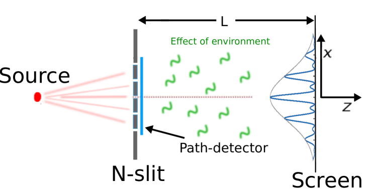
Figure 1: Schematic diagram of a n-slit interference experiment, with a quantum path-detector. The interfering particle is affected by interaction with an environment.

2 Multi-slit interference

2.1 Interference and path-detection

To set the ball rolling, let us first consider a quantum particle (quanton) passing through $n$-slits. If $|\psi_{i}\rangle$ represents the amplitude of the particle to pass through the $i$’th slit, then the state of the particle, after passing through the $n$ slits, can be described as a superposition of all possible amplitudes, i.e., $|\psi_{i}\rangle$, to go through different slits. The states $|\psi_{i}\rangle$ are mutually orthogonal by virtue of the slits being narrow and spatially separated. We choose $|\psi_{i}\rangle$ to be normalized, and associate a weight factor with it, which determines the probability of the particle to go through a particular slit:

$$|\Psi_{0}\rangle=c_{1}|\psi_{1}\rangle+c_{2}|\psi_{2}\rangle+\dots,c_{n}|\psi_{n}\rangle.$$ (3)

$|\Psi_{0}\rangle$ is normalized, and the sum of the probabilities $\sum_{i=1}^{n}|c_{i}|^{2}=1$. The probability density of the particle hitting the screen at a particular position $x$ on the screen (Fig.1) is given by $|\langle x|\Psi_{0}\rangle|^{2}$. The pattern on the screen has the following general form

$$|\langle x|\Psi_{0}\rangle|^{2}=\sum_{i=1}^{n}|c_{i}|^{2}|\langle x|\psi_{i}\rangle|^{2}+\sum_{j\neq k}c_{j}^{*}c_{k}\langle x|\psi_{k}\rangle\langle\psi_{j}|x\rangle.$$ (4)

The first term represents the sum of patterns formed by the particles coming out of individual slits, as if the other slits did not exist. The second term represents the interference between the amplitudes of particle coming out of j’th and k’th slits, summed over all j’s and k’s which are different. Clearly, the multi-slit interference pattern is built up of all possible two-slit inteference terms ($j\neq k$).

Since we are interested in probing which slit the particle went through, we need to have some kind of detector which does this job. We assume that our detector is the simplest, and is fully quantum mechanical. In the von Neumann scheme, measurements are described by treating both the system and the measuring apparatus (detector) as quantum objects and for a measurement to be affected, the measured system interacts with the detector to produce an entangled state with one-to-one correlations between the system and the detector states [15].

Thus, in order for the path-detector to be capable of detecting which of the $n$ paths the particle took, an entangled state of the following kind should result

$$|\Psi\rangle=c_{1}|\psi_{1}\rangle|d_{1}\rangle+c_{2}|\psi_{2}\rangle|d_{2}\rangle+\dots,c_{n}|\psi_{n}\rangle|d_{n}\rangle,$$ (5)

where $|d_{i}\rangle$ is the state of the path-detector if the quanton went through the $i$’th path. We choose the detector states $\{|d_{i}\rangle\}$ to be normalized, but not necessarily orthogonal. With the path-detector added to the interference setup, the pattern of the particles hitting the screen gets modified, and has the following form

$$|\langle x|\Psi_{0}\rangle|^{2}=\sum_{i=1}^{n}|c_{i}|^{2}|\langle x|\psi_{i}\rangle|^{2}+\sum_{j\neq k}c_{j}^{*}c_{k}\langle x|\psi_{k}\rangle\langle\psi_{j}|x\rangle\langle d_{j}|d_{k}\rangle.$$ (6)

From (6) one can see that the first term remains unaffected by the introduction of path-detector. This is obvious as the presence of a path detector is not expected to affect the probability of the particle to pass through a single slit. The second term, which gives rise to interference, however, is reduced by the factors $\langle d_{j}|d_{k}\rangle$. If the path-detector states are completely orthogonal, $\langle d_{j}|d_{k}\rangle=0$, it is clear from (6) that the interference term disappears. If the path-detector states are all identical, i.e., $\langle d_{j}|d_{k}\rangle=1$ for all $j,k$, (6) reduces to (4). This is in tune with the understanding that any attempt at gaining information about which slit the particle went through degrades the interference, while a complete ignorance about which-path information preserves the interference.

2.2 Effect of the environment

Let us now assume that as the particle (quanton) comes out of the n-slits and travels to the screen, it is affected by weak interaction with some kind of environment. We describe this environment as a reservoir of non-interacting quantum oscillators, each of which interacts with the particle. The Hamiltonian governing the particle can then be represented as

$$H=\frac{p^{2}}{2m}+\sum_{j}{P_{j}^{2}\over 2M_{j}}+{1\over 2}M_{j}\omega_{j}^{2}\left(X_{j}-{g_{j}x\over{M_{j}}\omega_{j}^{2}}\right)^{2},$$ (7)

where $x,p$ are the position and momentum operators of the particle (quanton), $m$ is its mass, $X_{j},P_{j}$ are position and momentum operators , and $M_{j}$ the mass of the jth harmonic oscillator of frequency $\omega_{j}$ comprising the environment and $g_{j}$ are the respective coupling strengths. The dynamics of a particle in simple potentials and in interaction with the environment modelled as a harmonic oscillator heat bath has been studied at great length in recent literature [16, 17, 18, 19, 20, 21]. The dynamics for the closed combine of the quanton and the environment is governed by the Hamiltonian evolution via (7) and the Schrödinger equation. A tracing over all the degrees of freedom of the environment results in an equation describing the dynamics of the reduced density matrix of just the quanton. This reduced density matrix evolves according to a master equation which is obtained by solving the Schrödinger equation for the particle and the environment and then tracing over the environment degrees of freedom. Several authors have worked extensively on the decoherence approach using the master equation for the reduced density matrix. The master equation for this kind of model of the environment was first derived separately by Caldeira and Leggett [16], Agarwal [17], Dekker [18] and others in the context of quantum Brownian motion and is popular in the study of open quantum systems. For our purpose, we deal with the master equation for the reduced density matrix for the particle (quanton) for the particle-environment composite described by (7), after the environment degrees of freedom are traced out:

$$\frac{\partial\rho(x,x^{\prime},t)}{\partial t} = \left\{\frac{-\hbar}{2im}\left(\frac{\partial^{2}}{\partial x^{2}}-\frac{\partial^{2}}{\partial x^{\prime 2}}\right)\right.$$

$$\left.-\gamma(x-x^{\prime})\left(\frac{\partial}{\partial x}-\frac{\partial}{\partial x^{\prime}}\right)-\frac{D}{4\hbar^{2}}(x-x^{\prime})^{2}\right\}.$$

(8)

Here $\rho(x,x^{\prime},t)$ is the reduced density matrix of the particle in the position degrees of freedom, $\gamma$ is the Langevin friction coefficient and $D=2m\gamma k_{B}T$ can be interpreted as a diffusion coeficient, and $T$ is the temperature of the harmonic oscillator heat-bath [16, 18, 17] . $\gamma$ and $D$ are related to the parameters of the total Hamiltonin (7). This master equation can be seen to naturally separate into three terms, one representing pure quantum evolution, one leading to dissipation or relaxation, and one causing diffusion. It has been widely reported in the literature that in the dynamics governed by such a master equation, coherent quantum superpositions persist for a very short time as they are rapidly destroyed by the action of the environment. It is generally agreed that the two main features seen as signatures of decoherence are : (a) the decoherence time, over which the superpositions decay is much much shorter than any characteristic time scale of the system (the thermal relaxation time, $\gamma^{-1})$, and (b) the decoherence time varies inversely as the square of a quantity that indicates the ‘size’ of the quantum superposition. This feature has also been reported in experiments [5, 6].

In the following we will attempt to quantify the effect of environment induce decoherence on a particle undergoing a n-slit inteference with the possibility of which path detection.

2.3 Decoherent dynamics of the particle

For calculational simplicity we assume that the state $|\psi_{k}\rangle$ which emerges from the k’th slit, is a Gaussian wave-packet localized at the location of the k’th slit, with a width equal to the width of the slit:

$$\langle x|\psi_{k}\rangle = \tfrac{1}{(\pi/2)^{1/4}\sqrt{\epsilon}}e^{-(x-k\ell)^{2}/\epsilon^{2}},$$ (9)

where $\ell$ is the distance between the centres of two neighboring slits, and $\epsilon$ is their approximate width. Following an interaction of the particle (quanton) with the which-path detector, the combined wave-function of the particle and the detector, as it emerges from the n-slits, is given by

$$\langle x|\Psi\rangle = \tfrac{1}{(\pi/2)^{1/4}\sqrt{\epsilon}}\sum_{k=1}^{n}c_{k}e^{-(x-k\ell)^{2}/\epsilon^{2}}|d_{k}\rangle,$$ (10)

which is a specific form of the entangled state (5). The density matrix corresponding to this can be written as

$$\rho_{0}(x,x^{\prime}) = \tfrac{1}{\sqrt{\pi/2}\epsilon}\sum_{j,k}c_{j}c_{k}^{*}e^{\frac{-(x-j\ell)^{2}}{\epsilon^{2}}}e^{\frac{-(x^{\prime}-k\ell)^{2}}{\epsilon^{2}}}|d_{j}\rangle\langle d_{k}|.~{}~{}~{}~{}$$ (11)

If one were to look only at the particle, it amounts to tracing over the states of the path detector, giving us the reduced density matrix for the quanton

$$\rho(x,x^{\prime},0) = \tfrac{1}{\sqrt{\pi/2}\epsilon}\sum_{j,k}c_{j}c_{k}^{*}e^{\frac{-(x-j\ell)^{2}}{\epsilon^{2}}}e^{\frac{-(x^{\prime}-k\ell)^{2}}{\epsilon^{2}}}\langle d_{k}|d_{j}\rangle.~{}~{}~{}~{}$$ (12)

This is the density operator of the particle at time $t=0$ as it emerges from the n-slit. Its decoherent dynamics will be governed by equation (8). We assume that after a time $t$ the particle reaches the screen, after traveling a distance $L$, and its density operator is given by $\rho(x,x^{\prime},t)$, described in the next section.

3 Results

3.1 Interference with decoherence

The measured intensity on the screen after the n-slits would be just the probability of the particle hitting the screen at a particular position. This, in turn, corresponds to the diagonal terms of the reduced density matrix of the particle, in the position basis. Eqn. (8) can be solved exactly, with the initial condition (12), to yield $\rho(x,x^{\prime},t)$. It’s diagonal component, $\rho(x,x,t)$, representing the probability density of the particle hitting the screen at a point $x$, is given by

$$\rho(x,x,t) = \frac{1}{\sqrt{\pi\alpha/2}}\left[\sum_{j=1}^{n}|c_{j}|^{2}e^{-{2(x-jl)^{2}\over\alpha}}\right.$$

$$\left.+\sum_{j\neq k}|c_{j}c_{k}||\langle d_{k}|d_{j}\rangle|e^{-\frac{1}{\alpha}f_{jk}(x)}\right.$$

$$\left.\cos\left\{\tfrac{2\hbar(1-e^{-2\gamma t})\ell(k-j)(x-\ell\frac{k+j}{2})}{\alpha\gamma m\epsilon^{2}}+\theta_{k}-\theta_{j}\right\}\right]$$

where
$f_{jk}(x)=(x-j\ell)^{2}+(x-k\ell)^{2}+\frac{l^{2}(j-k)^{2}D[4\gamma t+4e^{-2\gamma t}-e^{-4\gamma t}-3]}{16\epsilon^{2}m^{2}\gamma^{3}}$,
and $\alpha=\epsilon^{2}+\frac{\hbar^{2}(1-e^{-2\gamma t})^{2}}{\epsilon^{2}m^{2}\gamma^{2}}+\frac{D[4\gamma t+4e^{-2\gamma t}-e^{-4\gamma t}-3]}{8m^{2}\gamma^{3}}$. Also, for convenience, we have combined the phases of $c_{j}$ and $|d_{j}\rangle$ as $c_{j}|d_{j}\rangle=|c_{j}||d_{j}\rangle e^{i\theta_{j}}$ , where $|d_{j}\rangle$ is now real. Eqn. (11) represents the exact dynamics of a particle passing through a multi-slit with which path detection and interacting with an environment. It can be used to describe the dissipative dynamics of the particle. However, if one is interested in studying the effects of decoherence, one is in the limit of very weak coupling of the particle with the environment, where dissipative effects are negligible. Dissipation typically occurs at a time-scale of $1/\gamma$. We assume that the effect of the environment is so weak that dissipative time-scales are much longer than the time the particle takes to reach the screen, $t\ll 1/\gamma$, or $\gamma t\ll 1$. Further, it is assumed that the time evolution of the Gaussian can be calculated by either assuming the quanton to be a particle of mass $m$, moving with a momentum corresponding to a de Broglie wavelength $\lambda$, or by assuming it to be a photon of wavelength $\lambda$ [22] . We also assume the slit width to be very small, i.e., $\epsilon^{2}\ll\lambda L/\pi$. In this limit (11) reduces to

$$\rho(x,x,t) = \frac{1}{\sqrt{\pi\alpha/2}}\left[\sum_{j=1}^{n}|c_{j}|^{2}e^{-{2\epsilon^{2}(x-jl)^{2}/(\lambda L/\pi)}}\right.$$ (14)

$$+\left.\sum_{j\neq k}|c_{j}c_{k}||\langle d_{k}|d_{j}\rangle|e^{-\epsilon^{2}\{(x-j\ell)^{2}+(x-k\ell)^{2}\}\over(\lambda L/\pi)^{2}}{e^{\frac{-D(j-k)^{2}\ell^{2}t}{12\hbar^{2}}}}\right.$$

$$\left.\cos\left\{\frac{2\pi\ell(k-j)(x-\ell\frac{k+j}{2})}{\lambda L}+\theta_{k}-\theta_{j}\right\}\right],$$

As a consistency check, we first consider the limit of coupling with the environment going to zero, which is the regime when decoherence is completely absent. This is achieved by taking the limits $\gamma\to 0,~{}D\to 0$. In this limit, the term $e^{-D(j-k)^{2}\ell^{2}t/12\hbar^{2}}$ in (14) becomes equal to unity, and (14) reduces to eqn. (16) of ref. [13]. Thus in the limit of environmental coupling going to zero, we recover known results for n-slit interference.

Let us now analyze the implications of the result (14) in somewhat greater detail. Note that the decohering n-slit interference pattern (14) is also built up from all possible two-slit inteference terms as was the case in (4) when there was no coupling to the environment. The environmental coupling has had the effect of modifying these pair-wise contributions. The effect of decoherence is neatly condensed into the exponential factor $e^{-D(j-k)^{2}\ell^{2}t/12\hbar^{2}}$ multiplying the cosine term which gives rise to interference. It is evident that as time progresses, the decoherence effect will degrade the interference. One would naively think that the effect of environment will be to progressively decrease the contrast of the interference, while retaining its overall characteristic n-slit signature . However, the interesting point to notice here is that the exponential decay term in (14) cannot be pulled out of the summation, as it depends on j, k. It is worth reminding that the second summation term over j, k, ($j\neq k$) in (14) represents the interference between the amplitudes from the j’th and k’th slits. Here the argument of the exponent in the exponential decay term is $-D(j-k)^{2}\ell^{2}t/12\hbar^{2}$. Note that the distance between two pairs of slits is $(j-k)\ell$. Let us now understand the physical significance of this term. Clearly, the larger the difference between j and k, the smaller is the magnitude of the exponential decay term and hence the faster is the decay. This means that the decoherence effect has its strongest contributions coming from the interference from pairs of slits which are the farthest apart from each other and its weakest contributions for interference from neighboring pairs of slits which are next to each other. This is quite clearly in consonance with the accepted signatures of decoherence wherein the decoherence time varies inversely as the square of a quantity that indicates the ‘size’ of the quantum superposition [5, 6]. In our case this ’size’ is the distance between the two slits, $(j-k)\ell$. Notice that for each pair of slits, there will be a characteristic decoherence time, $\tau_{d}^{(jk)}=12\hbar^{2}/D(j-k)^{2}\ell^{2}$ and for n-slits there will be a total of n(n-1)/2 time scales which will collectively contribute in the summation leading to the degradation of the n-slit pattern. Of these terms, the strongest contribution to the fast exponential decay will come from one term corresponding to the pair of slits farthest apart. The weakest contributions will come from (n-1) terms for pairs of neighbouring slits and the coherence from their interfering amplitudes would survive the longest.

For the simplest case of two slits, there will be only one time scale, $\tau_{d}=12\hbar^{2}/D\ell^{2}$ = $\frac{6\hbar^{2}}{m\gamma k_{B}T\ell^{2}}$. A physical interpretation of this form of the decoherence time (leading to superpositions vanishing on a time scale much shorter than the relaxation time, $\gamma$) may be argued as stemming from the fact that in the model considered, the coordinate-coordinate coupling of the particle to the environment is very weak and the states of the environment correlated to the $n$ states of the particle emerging from the multi-slit, $|\psi_{1}\rangle,|\psi_{2}\rangle,...|\psi_{n}\rangle$ in (3), are mutually orthogonal to each other [16]. Eq. (14) summarizes the central result of this work, describing the interference pattern (position probability distribution) for a quanton interacting with an environment after emerging from n-slits with which way detectors. This result can be applied to recent experimental studies investigating entanglement, quantum coherence and decoherence in matter waves [24, 23].

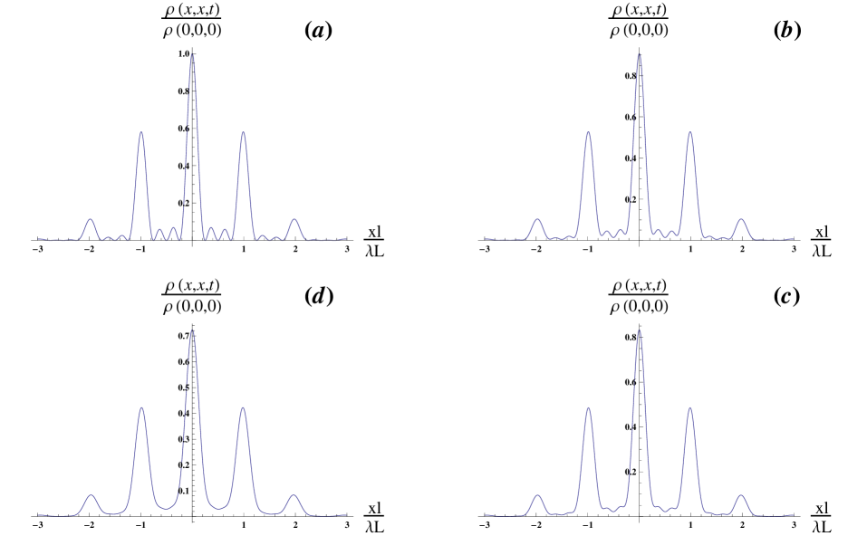
Figure 2: Plots of $\rho(x,x,t)/\rho(0,0,0)$ at the screen, for 4-slit interference, showing how decoherence progressively affects interference. The following parameters used are adapted from the interference experiment on ultracold Neon atoms [23]: $m=3.349\times 10^{-26}~{}\text{Kg},T=2.5~{}\text{mK},\lambda=0.018~{}\mu\text{m},\ell=6~{}\mu\text{m},L=37~{}\text{mm}$. The plots are for (a) $t/\tau_{d}=0$, (b) $t/\tau_{d}=1/24$, (c) $t/\tau_{d}=1/12$, (d) $t/\tau_{d}=1/6$, where $\tau_{d}=12\hbar^{2}/D\ell^{2}$. As decoherence effects set in, the multi-slit nature of the interference pattern disappears, and it is essentially reduced to a 2-slit interference pattern, as seen in (d).

Figures 2 and 3 illustrate the effect of decoherence as described by (14) for a simple example of four slits. We plot the position probability distribution (14) (interference pattern) with real parameters used in two significant experiments, the first by Shimizu et al [23] reporting the observation of matter wave interference of ultracold Neon atoms and the second by Arndt et al [24] which observes matter wave interference of $C_{60}$ molecules. One can see that decoherence leads to the washing out of the multi-slit character of the interference pattern first. Subsequently, the interference pattern essentially reduces to that of a 2-slit interference pattern. This aspect can be understood by recognizing that the strongest contribution to the decoherence comes from the two slits which are farthest apart, i.e., in this case slit number 1 and slit number 4. For interference between the amplitudes from these two widely separated slits, quantum coherence has to be maintained over a larger spatial distance. Since the time-scale over which coherence is destroyed between two spatially separated points is inversely proportional to the square of their separation, the coherence between slit 1 and slit 4 in our example is destroyed faster. Since the weakest contribution to decoherence comes from the interfering amplitudes between nearest neighbour pairs of slits, the four-slit pattern decays to a two-slit interference pattern whose coherence is destroyed much more slowly. With the passage of time, decoherence eventually leads to a further loss in contrast and the eventual washing away of the fringes [25](see Figure 3). Figure 4 illustrates this for five-slit interference. In fact it can be shown that irrespective of the number of slits, all n-slit patterns, when affected by decoherence, degrade over time to a two-slit interference pattern which eventually washes away. It should be mentioned here that in this discussion, we are using the term coherence only in a qualitative sense, and not the one defined by (1).

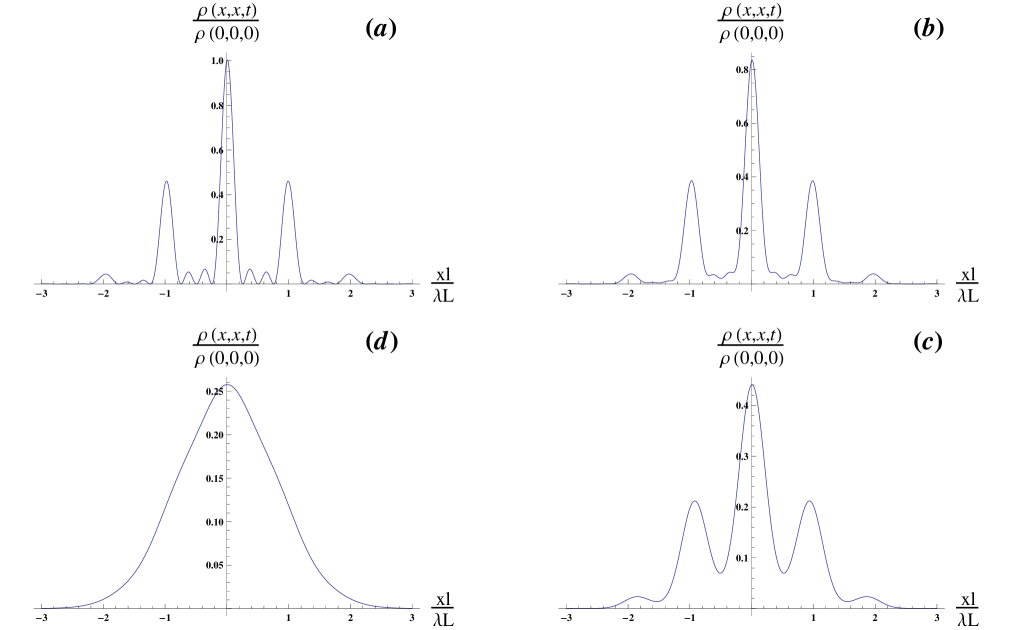
Figure 3: Plots of $\rho(x,x,t)/\rho(0,0,0)$, at the screen, for 4-slit interference, showing how decoherence progressively affects interference. The following parameters used are adapted from the interference experiment with $C_{60}$ molecules [24]: $m=1.2\times 10^{-24}~{}\text{Kg},T=900~{}\text{K},\lambda=0.0025~{}\text{nm},\ell=100~{}\text{nm},L=1.25~{}\text{m}$. The plots are for (a) $t/\tau_{d}=0$, (b) $t/\tau_{d}=1/12$, (c) $t/\tau_{d}=3/4$, (d) $t/\tau_{d}=4$, where $\tau_{d}=12\hbar^{2}/D\ell^{2}$. As decoherence effects set in, the multi-slit nature of the interference pattern disappears first, and it is essentially reduced to a 2-slit interference pattern, as seen in (b). With stronger decoherence effects, the effective 2-slit interference pattern is also washed out.

3.2 Measuring coherence

Next we turn to quantitatively extracting the coherence $\mathcal{C}$ [12] as defined in (1) from the interference in (11) or (14). In order to measure coherence from a n-slit interference, we need to have such a path detector in place whose path-distinguishability is tunable [13]. The minimum requirement is that it should be switchable between two modes corresponding to (a) making all the paths completely indistinguishable and (b) making all the paths fully distinguishable. We denote the two cases (a) and (b) by $\parallel$ and $\perp$, respectively. The procedure is as follows. First, the intensity at a primary maximum $I_{max}^{\parallel}$ is measured when the n paths are indistinguishable, i.e., $|d_{i}\rangle$s are all identical and parallel. Next, the path-detector is switched to the mode (b) where all the n paths are fully distinguishable, and the intensity $I_{max}^{\perp}$ is measured at the same location on the screen as before.

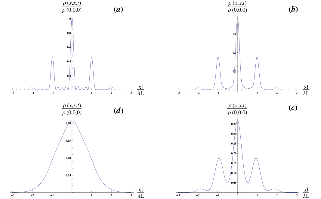
Figure 4: Plots of $\rho(x,x,t)/\rho(0,0,0)$, at the screen, for 5-slit interference, showing how decoherence progressively affects interference. The following parameters used are adapted from the interference experiment with $C_{60}$ molecules [24]: $m=1.2\times 10^{-24}~{}\text{Kg},T=900~{}\text{K},\lambda=0.0025~{}\text{nm},\ell=100~{}\text{nm},L=1.25~{}\text{m}$. The plots are for (a) $t/\tau_{d}=0$, (b) $t/\tau_{d}=1/12$, (c) $t/\tau_{d}=3/4$, (d) $t/\tau_{d}=4$, where $\tau_{d}=12\hbar^{2}/D\ell^{2}$. As decoherence effects set in, the multi-slit nature of the interference pattern disappears first, and it is essentially reduced to a 2-slit interference pattern, as seen in (b). With stronger decoherence effects, the effective 2-slit interference pattern is also washed out.

Coherence of the incoming particles can then be measured as [13]

$$\mathcal{C}_{expt}=\frac{1}{n-1}\frac{I_{max}^{\parallel}-I_{max}^{\perp}}{I_{max}^{\perp}}.$$ (15)

In order to extract $\mathcal{C}$ from (14), we assume that the width of the slits $\epsilon$ is very narrow, and the narrow width Gaussians $e^{{-(x-j\ell)^{2}}/{\epsilon^{2}}}$ in (12), become very wide $e^{-{2\epsilon^{2}(x-jl)^{2}/(\lambda L/\pi)^{2}}}$ in (14), as the particle reaches the screen. This is the Fraunhofer limit $\epsilon^{2}/\lambda L\ll 1$, and is satisfied by the real experimental parameters used in Figures 2, 3 and 4. Terms like $e^{-{2\epsilon^{2}(x-jl)^{2}/(\lambda L/\pi)^{2}}}$ are wide Gaussians, whose centers are shifted by tiny amounts of the order of a few slit-separations. For all practical purposes, the values of all the Gaussians, at any point $x$ on the screen, is almost the same, and thus independent of $j,k$. We denote it by $g(x)\equiv e^{-{2\epsilon^{2}(x-jl)^{2}/(\lambda L/\pi)}}$. The expression for $\rho(x,x,t)$ is then approximated as

$$\rho(x,x,t) \approx \frac{g(x)}{\sqrt{\pi\alpha/2}}\left[\sum_{j=1}^{n}|c_{j}|^{2}+\sum_{j\neq k}|c_{j}c_{k}||\langle d_{k}|d_{j}\rangle|{e^{-(j-k)^{2}t/\tau_{d}}}\right.$$ (16)

$$\left.\cos\left\{\frac{2\pi\ell(k-j)(x-\ell\frac{k+j}{2})}{\lambda L}+\theta_{k}-\theta_{j}\right\}\right].$$

Now, in a n-slit interference, the primary maxima are at those points on the screen where the value of all the cosine terms is 1, irrespective of the values of j, k. From (16) one can get the expressions for $I_{max}^{\parallel}$ and $I_{max}^{\perp}$ as follows:

$$I_{max}^{\parallel} = \frac{g(x)}{\sqrt{\pi\alpha/2}}\left[\sum_{j=1}^{n}|c_{j}|^{2}+\sum_{j\neq k}|c_{j}c_{k}|e^{-(j-k)^{2}t/\tau_{d}}\right]$$

$$I_{max}^{\perp} = \frac{g(x)}{\sqrt{\pi\alpha/2}}\left[\sum_{j=1}^{n}|c_{j}|^{2}\right].$$ (17)

Coherence can then be calculated using (15):

$$\mathcal{C} = \frac{1}{n-1}\sum_{j\neq k}|c_{j}c_{k}|{e^{-(j-k)^{2}t/\tau_{d}}}$$ (18)

$$= \frac{1}{n-1}\sum_{j\neq k}|c_{j}c_{k}|\exp\left\{\frac{-(j-k)^{2}\ell^{2}tm\gamma k_{B}T}{6\hbar^{2}}\right\},$$

where we have used the property $\sum_{j=1}^{n}|c_{j}|^{2}=1$. Eqn. (18) is interesting as it quantitatively captures the coherence of the quanton in terms of real parameters of the environment and its coupling. For example, it quantifies the effect of increasing or decreasing the temperature of the heat-bath on the coherence of the particle. This feature can be experimentally tested in matter wave interference experiments by changing the temperature of the ambient gas reservoir [26]. Note that while the interference pattern captured by (14) depends on the overlaps of the path-detector states, the coherence represented by (18), is completely independent of the path detector.

The two-slit ($n=2$) case is particularly useful, as we shall see in the following. For $n=2$, (18) reduces to

$$\mathcal{C} = 2|c_{1}c_{2}|{e^{-t/\tau_{d}}}.$$ (19)

This immediately allows us to represent the decoherence time, $\tau_{d}$, in terms of the coherence , $\mathcal{C}$, as

$${\tau_{d}}=\frac{t}{\log(2|c_{1}c_{2}|/\mathcal{C})},$$ (20)

or

$${\tau_{d}}=\frac{\lambda Lm/h}{\log(2|c_{1}c_{2}|/\mathcal{C})}.$$ (21)

The above expression can be extremely useful for the following reason. In a two-slit interference experiment, if one can experimentally measure coherence using (15), it allows one to determine the decoherence time. For instance, one may be interested in knowing the decoherence time-scale in a particular experimental situation, limited by the degree of vacuum and other constraints. For example, if one can hook up a symmetric two-slit interference experiment, with which-way detection, it allows one to experimentally determine the decoherence time-scale simply by using the following relation:

$${\tau_{d}}=\frac{\lambda Lm/h}{\log\left(\frac{I_{max}^{\perp}}{I_{max}^{\parallel}-I_{max}^{\perp}}\right)}.$$ (22)

Thus decoherence can be monitored by measuring intensities in the interference pattern. While considerable progress in the theoretical understanding of decoherence has been made in recent times, experiments that can control environmental coupling and monitor progressive decoherence are few [6, 4]. In particular, measurement of the decoherence time in various situations remains a big challenge. Knowledge of the decoherence time is crucial in systems where quantum coherence is exploited for information processing and computing, making (22) an extremely useful result.

4 Conclusions

We have theoretically analyzed a multi-slit interference with which-way detection, in the presence of environment-induced decoherence. Decoherence degrades the interference in an interesting manner, with the multi-slit features disappearing first, and the interference pattern reducing to an effective decohering two-slit interference pattern, which eventually washes out. An analytical expression for the coherence of the interfering particle is obtained in terms of the parameters of the environment and the particle-environment coupling. Using that we show that decoherence can be quantified by measuring coherence. For the particular case of two-slit interference, we show that the decoherence time-scale can be experimentally determined by measuring coherence, which in turn, can be determined by measuring interference intensities in a particular way.This procedure may become useful in developing methods of monitoring decoherence in many potentially useful quantum systems which exploit quantum coherence.

References

- [1] E. Joos, H. D. Zeh, C. Kiefer, D. J. Giulini, J. Kupsch, and I. O. Stamatescu, Decoherence and the appearance of a classical world in quantum theory (Springer, 1996).
- [2] W. H. Zurek, Physics Today 44 (10), 36 (1991).
- [3] M. Schlosshauer, Decoherence and the Quantum-to-Classical Transition ( Berlin/Heidelberg: Springer, 2007 ), edition.
- [4] C. Monroe, D. M. Meekhof, B. E. King, and D. J. Wineland, Science 272, 1131 (1996).
- [5] M. Brune, E. Hagley, J. Dreyer, X. Maître, A. Maali, C. Wunderlich, J. M. Raimond, and S. Haroche, Phys. Rev. Lett. 77, 4887-4890 (1996).
- [6] C. Monroe, D. Wineland, S. Haroche, and J. Raimond, Physics Today 49 (11), 107 (1996).
- [7] M. H. S. Amin, C. J. S. Truncik, and D. V. Averin, Phys. Rev. A 80, 022303 (2009).
- [8] S. Ashhab, J. R. Johansson, and Franco Nori, Phys. Rev. A 74, 052330 (2006).
- [9] M. S. Byrd and D. A. Lidar, Phys. Rev. Lett. 89, 047901 (2002).
- [10] W. H. Zurek, Phys. Rev. D 26(8), 1862 (1982).
- [11] T. Baumgratz, M. Cramer, and M. B. Plenio, Phys. Rev. Lett. 113, 140401 (2014).
- [12] M. N. Bera, T. Qureshi, M. A. Siddiqui, and A. K. Pati, Phys. Rev. A 92, 012118 (2015).
- [13] T. Paul and T. Qureshi, Phys. Rev. A 95, 042110 (2017).
- [14] T. Biswas, M. G. Díaz, A. Winter, Proc. R. Soc. A 473, 20170170 (2017).
- [15] J. von Neumann, Mathematical Foundations of Quantum Mechanics (Princeton University Press, 1955).
- [16] A. O. Caldeira and A. J. Leggett, Physica A 121, 587 (1983); Phys. Rev. A 31, 1059 (1985).
- [17] G. S. Agarwal, Phys. Rev. A 4, 739-747 (1971).
- [18] H. Dekker, Phys. Rep. 80, 1 (1981); Phys. Rev. A 16, 2116 (1977).
- [19] A. Barchielli, L. Lanz and G. M. Prosperi, Nuovo Cimento 72B, 79 (1982); Found. Phys. 13, 779 (1983).
- [20] D. Kumar, Phys. Rev. A 29, 1571 (1984).
- [21] A. Venugopalan, D. Kumar and R. Ghosh, Physica A 220, 568 (1995); A. Venugopalan, Phys. Rev. A 56, 4307 (1997); A. Venugopalan, ibid. 61, 012102 (2000).
- [22] G. Dillon, Eur. Phys. J. Plus 127, 66 (2012).
- [23] F. Shimizu, K. Shimizu, and H. Takuma, Phys. Rev. A 46, R17–R20 (1992).
- [24] M. Arndt, O. Nairz, J. Vos-Andreae, C. Keller, G. van der Zouw, and A. Zeilinger, Nature 401, 680 (1999).
- [25] T. Qureshi and A. Venugopalan, Int. J. Mod. Phys. B 22, 981 (2008).
- [26] K. Hornberger, S. Gerlich, P. Haslinger, S. Nimmrichter, and M. Arndt, Rev. Mod. Phys. 84, 157 (2012).