Observability inequalities for transport equations through Carleman estimates

Abstract

We consider the transport equation $\partial_{t}u(x,t)+H(t)\cdot\nabla u(x,t)=0$ in $\Omega\times(0,T),$ where $T>0$ and $\Omega\subset\mathbb{R}^{d}$ is a bounded domain with smooth boundary $\partial\Omega$. First, we prove a Carleman estimate for solutions of finite energy with piecewise continuous weight functions. Then, under a further condition which guarantees that the orbits of $H$ intersect $\partial\Omega$, we prove an energy estimate which in turn yields an observability inequality. Our results are motivated by applications to inverse problems.

1 Introduction

Let $d\in\mathbb{N}$ and $\Omega\subset\mathbb{R}^{d}$ be a bounded domain with smooth boundary $\partial\Omega$, $\nu=\nu(x)$ be the unit outward normal vector at $x$ to $\partial\Omega$, and let $x\cdot y$ and $|x|$ denote the scalar product of $x,y\in\mathbb{R}^{d}$ and the norm of $x\in\mathbb{R}^{d},$ respectively. We set $Q:=\Omega\times(0,T),$ and we consider

$$Pu(x,t):=\partial_{t}u+H(t)\cdot\nabla u=0\quad\mbox{in $Q$},$$ (1)

where $H(t):=(H_{1}(t),\ldots,H_{d}(t)):[0,T]\rightarrow\mathbb{R}^{d},$  $H\in C^{1}([0,T];\mathbb{R}^{d})$.

Equation (1) is called a transport equation and $H(t)$ describes the velocity of the flow, which is here assumed to be independent of the spatial variable $x$.

Problem formulation

We assume

$$H_{0}:=\min_{t\in[0,T]}|H(t)|>0,$$ (2)

and, without loss of generality, we suppose that ${\bf 0}=(0,\ldots,0)\in\overline{\Omega}.$

Let us recall the following definition.

Definition 1.1

A partition $\{t_{j}\}_{0}^{m}$ of $[0,T]$ is a strictly increasing finite sequence $t_{0},t_{1},\ldots,t_{m}$ (for some $m\in\mathbb{N}$) of real numbers starting from the initial point $t_{0}=0$ and arriving at the final point $t_{m}=T.$

Hereafter, we will call $\{t_{j}\}_{0}^{m}$ a uniform partition of $[0,T]$ when the length of the intervals $[t_{j},t_{j+1}]$ is constant for $j=0,\ldots,m-1,$ that is, $t_{j}=\frac{T}{m}j,\;\;j=0,\ldots,m.$

Lemma 1.2 below ensures that any vector-valued function $H(t),$ satisfying (2), admits a partition $\{t_{j}\}_{0}^{m}$ of $[0,T]$ such that the angles of oscillations of the vector $H(t)$ are less than $\frac{\pi}{2}$ in any time interval $[t_{j},t_{j+1}],\;j=0,\ldots,m-1$ (see Figure 1).

Given a partition $\{t_{j}\}_{0}^{m}$ of $[0,T],$ let us set

$$\eta_{j}:=\frac{H(t_{j})}{|H(t_{j})|},\;\;\;j=0,\ldots,m-1.$$ (3)

Lemma 1.2

Let  $S_{*}\in(1/\sqrt{2},1).$ For any given $H\in Lip([0,T];\mathbb{R}^{d})$, satisfying condition (2), there exist $m\in\mathbb{N}$ and a partition $\{t_{j}\}_{0}^{m}$ of $[0,T]$ such that

$$\frac{H(t)}{|H(t)|}\cdot\eta_{j}\geq S_{*},\;\;\;\forall t\in[t_{j},t_{j+1}],\;\;\forall j=0,\ldots,m-1,$$ (4)

where $\eta_{j}$ are defined in (3).

Lemma 1.2 is proved in the Appendix.

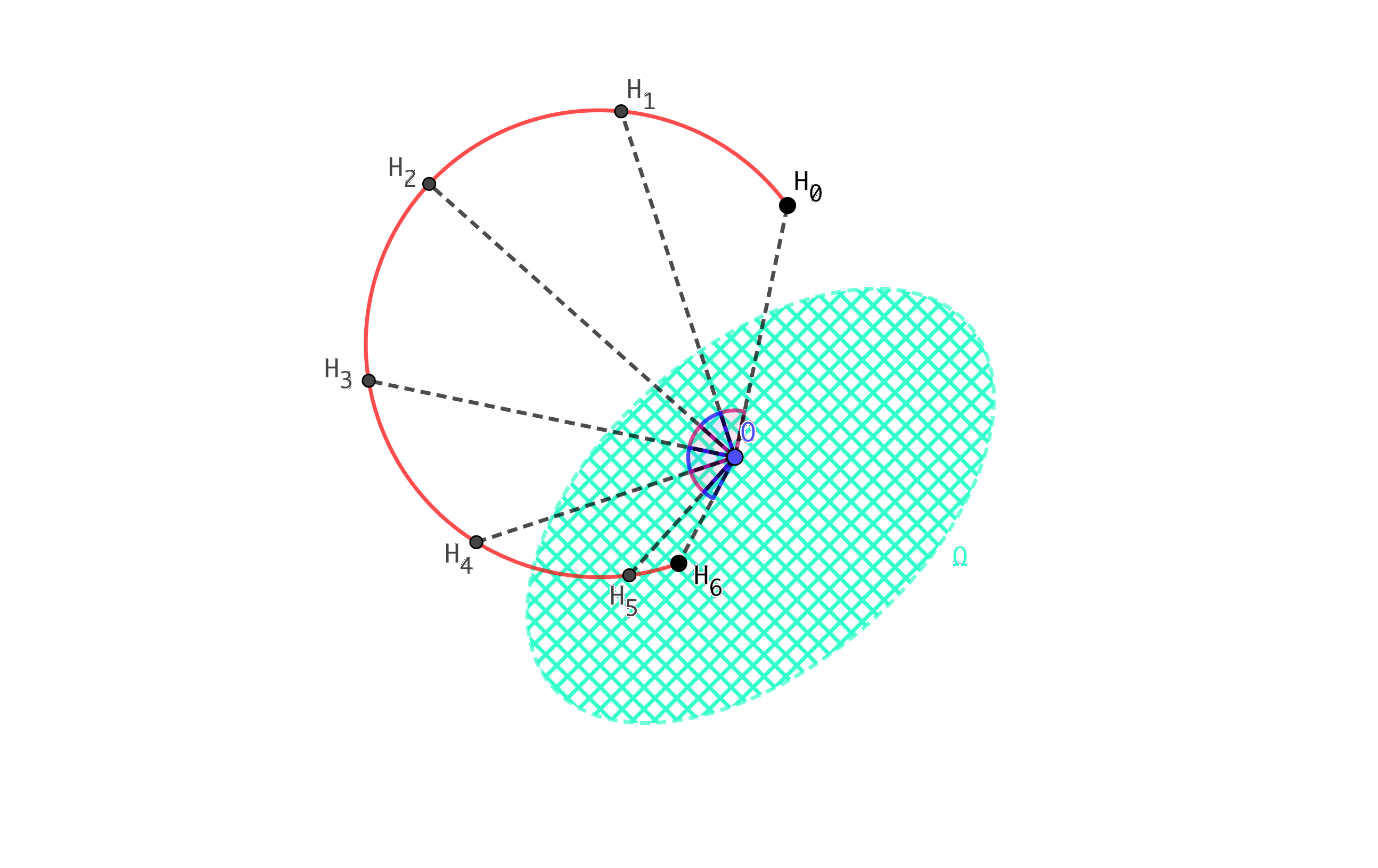
Figure 1: In this picture $S_{*}=\cos\frac{\pi}{6},\>m=6$ and $H_{j}:=H(t_{j}),\,j=0,\ldots,5.$

Remark 1.3

Condition (4) means that there exist $m$ cones in $\mathbb{R}^{d}$ such that the axis of every cone, that is, the straight line passing through the apex about which the whole cone has a circular symmetry, is the line between $O=(0,\ldots,0)$ and $\eta_{j},\;j=0,\ldots,m-1$. Moreover, a straight line passing through the apex is contained in the cone if the angle between this line and the axis of the cone is less than $\pi/4$. Indeed, the inequality (4), that is $H(t)\cdot\eta_{j}>\cos\vartheta^{*}|H(t)|$ for some $\vartheta^{*}\in(0,\frac{\pi}{4}),$ is equivalent to the fact that the angle between $H(t)$ and $\eta_{j}$ is less than $\pi/4.$ Thus, $H(t)$ is contained in the same cone $\forall t\in[t_{j},t_{j+1}].$ Let us note that it can occur that $\eta_{i}=\eta_{j},$ for $i\neq j.$

Let $\delta_{\Omega}=diam(\Omega)=\displaystyle\sup_{x,y\in\overline{\Omega}}|x-y|.$ Let us fix $S_{*}\in(1/\sqrt{2},1),$ $r>0$ and define

$$x_{j}:=-R_{j}\eta_{j},\;\;\;j=0,\ldots,m-1,$$ (5)

where $\eta_{j}$ is defined in (3) and

$$\left\{\begin{array}[]{rl}R_{j}&=2^{j}R_{0}+(2^{j}-1)(\delta_{\Omega}+r),\\ R_{0}&=\frac{1+S_{*}}{1-S_{*}}\delta_{\Omega}.\end{array}\right.$$ (6)

We note that from (6) it follows that

$$x_{j}\not\in\overline{\Omega},\qquad j=0,\ldots,m-1.$$

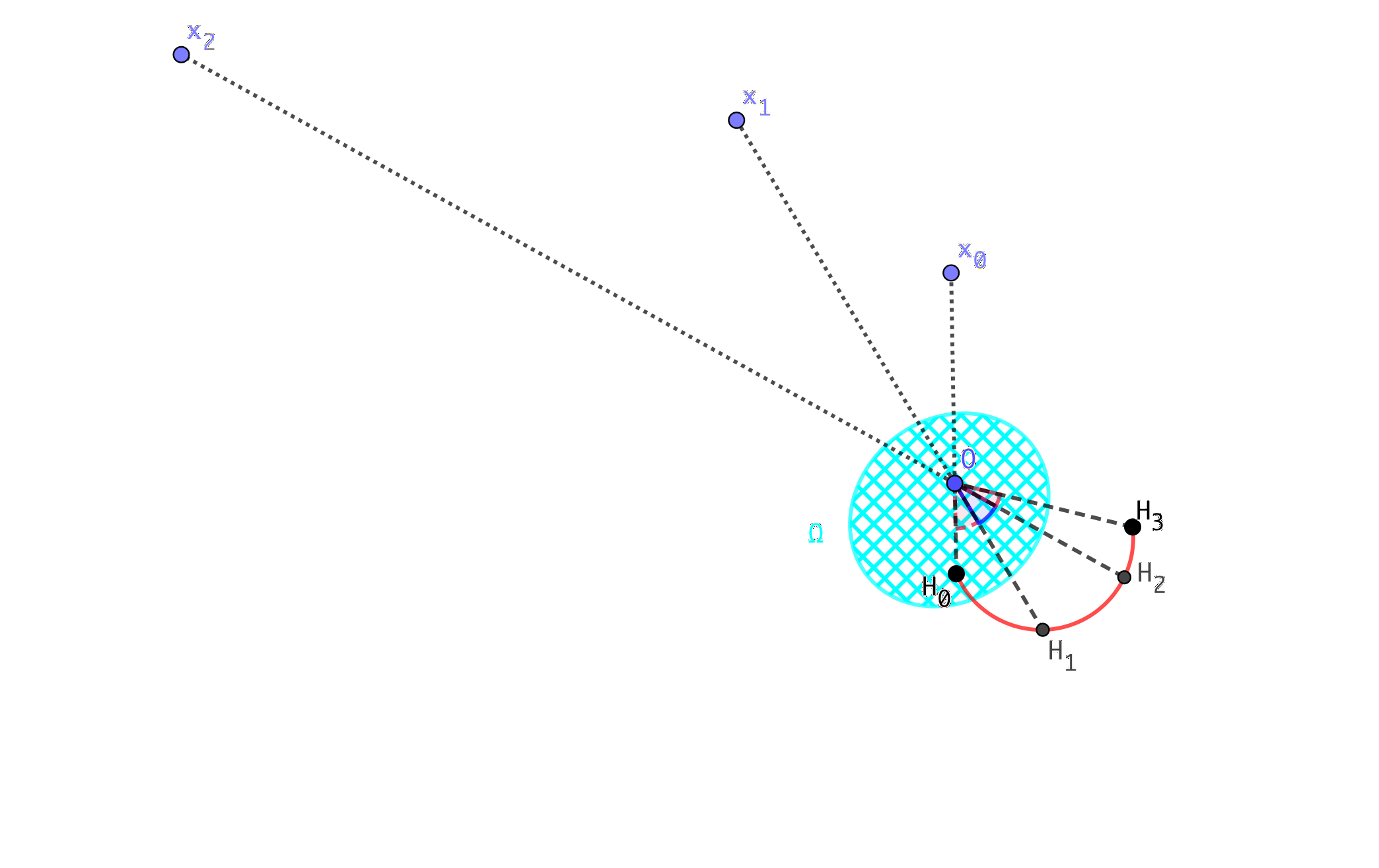
Figure 2: In this picture $S_{*}=\cos\frac{\pi}{6},\>m=3$ and $H_{j}:=H(t_{j}),\,j=0,1,2.$

For every $j=0,\ldots,m-1,$ let us define

$$M_{\Omega}(x_{j}):=\max_{x\in\overline{\Omega}}|x-x_{j}|\qquad\mbox{ and }\qquad d_{\Omega}(x_{j}):=\min_{x\in\overline{\Omega}}|x-x_{j}|.$$ (7)

Remark 1.4

The choice of the $R_{j}$’s in (6) (see Lemma 2.2 below and Figure 2) guarantees that the points $x_{j}$’s are located sufficiently far away from $\Omega$ and at increasing distances from the origin.

By the choice of the finite sequence $R_{j}=|x_{j}|$ in (6) ($R_{j}$ sufficiently large compared with $\delta_{\Omega}$) we deduce in Lemma 2.1 below that

$$(x+R_{j}\eta_{j})\cdot\eta_{j}\geq S_{*}|x+R_{j}\eta_{j}|,\;\;\forall x\in\overline{\Omega}.$$

In other words, the apex angle of the minimum cone with the apex $x_{j}$ which includes $\Omega$ is less than $2\arccos S_{*}(<\pi/2)$ (see Figure 3).

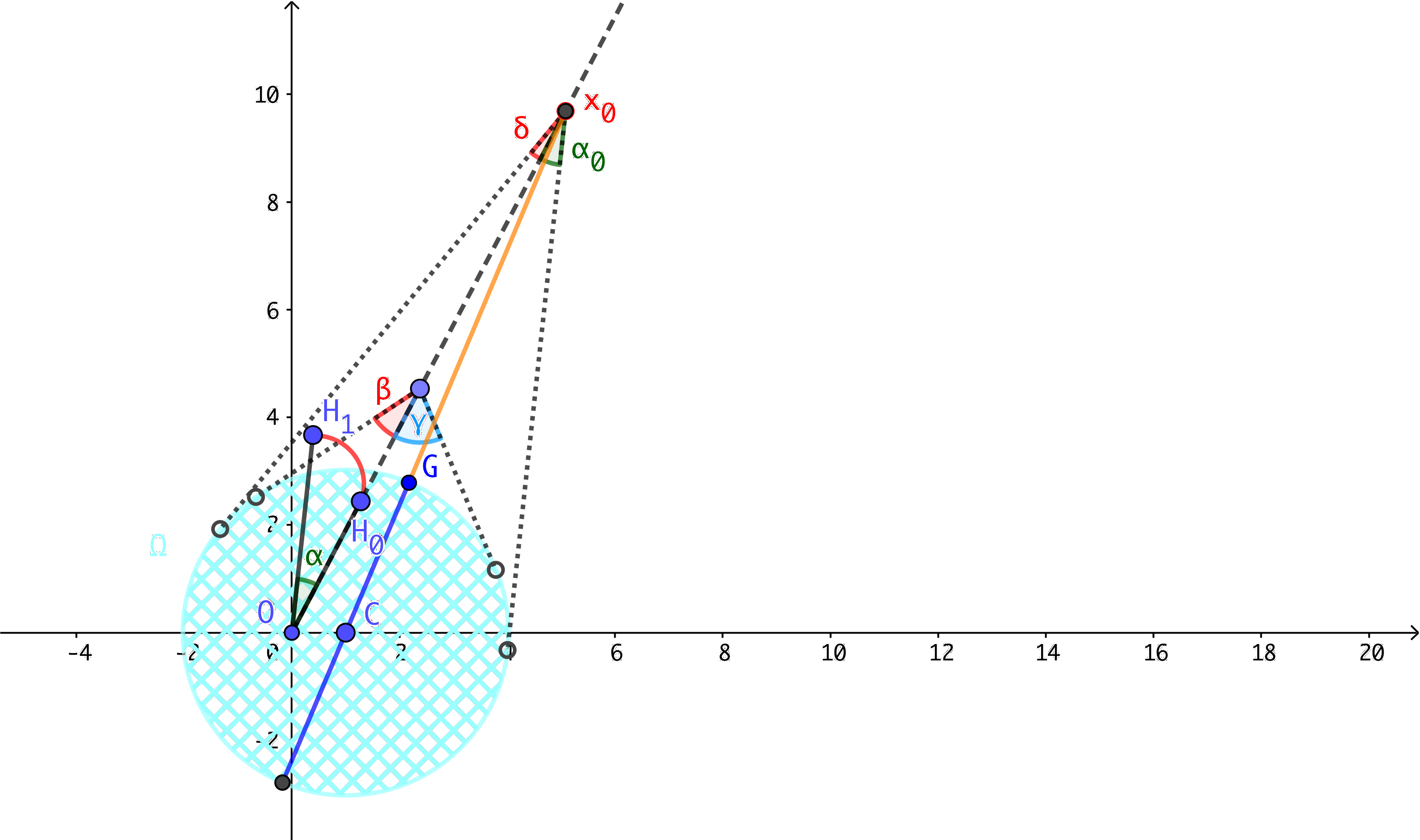
Figure 3: In this picture: $\Omega:=\{(x,y)\in R^{2}:|(x,y)-(1,0)|<3\},\>C=(1,0),$  $S_{*}=\cos\alpha\in(\frac{1}{\sqrt{2}},1),\>m=1,$ $H_{j}:=H(t_{j}),\,j=0,1,$ and $\beta,\gamma>\alpha,\,\alpha_{0}=\alpha,\delta\leq\alpha.$ We note that $d_{\Omega}(x_{0})=\mathrm{dist}\,(x_{0},G)$ and $M_{\Omega}(x_{0})=d_{\Omega}(x_{0})+6.$

We now introduce the weight function $\varphi(x,t)$, to be used in our Carleman estimate, as follows. First, we define $\varphi$ on $\overline{\Omega}\times[0,T)$ setting, for every $x\in\overline{\Omega},$

$$\varphi(x,t)=\varphi_{j}(x,t):=-\beta(t-t_{j})+|x-x_{j}|^{2},\;\;t\in[t_{j},t_{j+1}),\;j=0,\ldots,m-1,$$ (8)

where

$$\beta:=(2S_{*}^{2}-1)H_{0}d_{\Omega}(x_{0}),$$ (9)

with $H_{0}$ and $d_{\Omega}(x_{0})$ defined by (2) and $(\ref{wf4}),$ respectively. Then we extend $\varphi$ to $\overline{\Omega}\times[0,T]$ by continuity. Observe that $\varphi$ is piecewise smooth in $t$ and smooth in $x$.

Main results

In this article, under condition (2), we establish an observability inequality for (1) which estimates the $L^{2}$-norm of $u(x,0)$ by lateral boundary data $u|_{\partial\Omega\times(0,T)}$ under some conditions on $H(t)$ (see Theorem 1.6). This observability inequality is a consequence of the following Carleman estimate.

Theorem 1.5

Let $u\in H^{1}(Q)$ be a solution of equation (1), where $H\in C^{1}([0,T];\mathbb{R}^{d})$ satisfies (2). Let $\{t_{j}\}_{0}^{m}$ be a partition of $[0,T]$ satisfying (4). Then, there exist constants $s_{0},C_{0},C>0$ such that for all $s>s_{0}$ we have

$$s^{2}\!\!\!\!\!\!\!\!\! \int_{Q}|u|^{2}e^{2s\varphi}dxdt+se^{-C_{0}s}\sum_{j=0}^{m-1}\int_{\Omega}|u(x,t_{j})|^{2}dx$$

$$\leq C\int_{Q}|Pu|^{2}e^{2s\varphi}dxdt+Cse^{Cs}\int_{\Sigma}|u|^{2}d\gamma dt+Cse^{Cs}\int_{\Omega}|u(x,T)|^{2}\,dx,$$

where $\varphi(x,t):Q\longrightarrow\mathbb{R}$ is the weight function defined in (8), and

$$\Sigma=\{(x,t)\in\partial\Omega\times(0,T):\,\thinspace H(t)\cdot\nu(x)\geq 0\}$$ (10)

is the subboundary of all exit points for $H$.

We now give the observability inequality for the equation (1).

Theorem 1.6

Let $g\in L^{2}(\partial\Omega\times(0,T))$ and let us consider the following problem

$$\left\{\begin{array}[]{rl}&\partial_{t}u+H(t)\cdot\nabla u=0\quad\mbox{in $Q:=\Omega\times(0,T)$},\\ &u|_{\partial\Omega\times(0,T)}=g.\end{array}\right.$$ (11)

Let us suppose that there exists a partition $\{t_{j}\}_{0}^{m}$ of $[0,T]$ associated to $H(t)$ satisfying (4) such that the following condition holds

$$\max_{0\leq j\leq m-1}\frac{(t_{j+1}-t_{j})d_{\Omega}(x_{j})}{M^{2}_{\Omega}(x_{j})}>\frac{1}{H_{0}(2S_{*}^{2}-1)},$$ (12)

where $M_{\Omega}(x_{j}),d_{\Omega}(x_{j})$ and $H_{0}$ are defined in $(\ref{wf4})$ and $(\ref{H1}),$ respectively. Then, there exists a constant $C>0$ such that the following inequality holds

$$\|u(\cdot,t)\|_{L^{2}(\Omega)}\leq C\|g\|_{L^{2}(\partial\Omega\times(0,T))},\quad 0\leq t\leq T,$$

for any $u\in H^{1}(Q)$ satisfying (11).

Assumption (12) is meant to guarantee that the orbit $\{H(t)\in\mathbb{R}^{d}~{}:~{}t\in[0,T]\}$ intersects $\partial\Omega.$ In the following example, we show that this or a similiar condition is indeed necessary: observability fails without some extra assumption.

In the following, for $\eta>0$ we consider $\Omega_{\eta}:=\{z\in\mathbb{R}^{2}:\,|z|<\eta\}.$

Example 1

Let $\sigma>0$ and $\rho\in(0,2\sigma/3).$ Let $\Omega:=\Omega_{\rho}$ and let $f\in C^{1}(\overline{\Omega}_{\sigma};\mathbb{R})$ be such that $\mathop{\rm supp}(f)\subset\Omega_{\rho/2}\subseteq\overline{\Omega}_{\sigma}$ and let $\alpha(t)=(\rho\cos t,\rho\sin t),\,t\in[0,2\pi].$ We set

$$v(x,y,t)=f(x-\rho\cos t,y-\rho\sin t).$$

Thus, $v$ satisfies (1), where $H(t)=\alpha^{\prime}(t)$, $0\leq t\leq T$, and $v$ vanishes at the boundary of $\Omega_{\sigma}$. So,

$$\left\{\begin{array}[]{rl}&\partial_{t}v+\alpha^{\prime}(t)\cdot\nabla v=0\quad\mbox{in $\Omega_{\sigma}\times(0,T)$},\\ &v|_{\partial\Omega_{\sigma}\times(0,T)}=g,\end{array}\right.$$ (13)

with $g\equiv 0.$ We note that $|\alpha^{\prime}(t)|=\rho>0$ and, for $t\in[0,T]$, the support of $v(\cdot,\cdot,t)$ is

$$\mathop{\rm supp}(v(\cdot,\cdot,t))=\left\{(x,y)\in\mathbb{R}^{2}:\,\left|(x-\rho\cos t,y-\rho\sin t)\right|<\frac{\rho}{2}\right\}.$$ (14)

Then, from (13) and (14) it follows that observability fails. $\square$

We conclude this introduction with some comments on our main results.

1. One could establish an estimate similar to the one in Theorem 1.6 with the maximum norm by the method of characteristics. Our proof is based on Carleman estimates, which naturally provide $L^{2}$-estimates for solutions over $\Omega\times\{t\}$. The method of characteristics does not yield such global $L^{2}$-estimates directly. $L^{2}$-estimates, not estimates in the maximum norm, are related to exact controllability and are more flexibly applied to other problems such as inverse problems, although we discuss no such aspects in this paper.

2. Although, due to the simplicity of equation (1), the method of characteristics can be easily applied to explain the validity of observability results, the one point we would like to stress is the fact that, in this paper, we intend to derive a Carleman estimate under minimal assumptions. Essentially, we want to give an explicit construction of the weight function that only depends on the lower bound (2) and the modulus of continuity of $H.$

3. It is worth noting that Theorem 1.6 aims at the determination of the solution $u$ on the whole cylinder $\Omega\times[0,T]$, not only of $u(\cdot,0)$ in $\Omega$. For this reason, in Theorem 1.6, we have to measure data on the whole lateral boundary $\partial\Omega\times(0,T)$, not just on a subboundary as we did for the Carleman estimate in Theorem 1.5—where, however, the norm of $u(\cdot,T)$ in $\Omega$ is included. The fact that measurements on the whole boundary are necessary to majorize $u$ on $\Omega\times[0,T]$ can be easily understood by looking at the representation solutions given by characteristics.

4. Another purpose of this paper is to single out an assumption which suffices to derive observability from a Carleman estimate. We do so with condition (12), which has a clear geometric meaning: one requires $H(t)$ not to oscillate too much for enough time, giving an explicit evaluation of such a time. We do not pretend our method to provide the optimal evaluation of the observability time. On the other hand, Example 1 shows that some assumption is needed for observability: (12) is an example of a sufficient quantitative condition for the observability of solutions on $\Omega\times[0,T]$.

Main references and outline of the paper

Carleman estimates for transport equations are proved in Gaitan and Ouzzane GO , Gölgeleyen and Yamamoto GY , Klibanov and Pamyatnykh KP , Machida and Yamamoto MM to be applied to inverse problems of determining spatially varying coefficients, where coefficients of the first-order terms in $x$ are assumed not to depend on $t$. In order to improve results for inverse problems by the application of Carleman estimates, we need a better choice of the weight function in the Carleman estimate. The works GO and KP use one weight function which is very conventional for a second-order hyperbolic equation but seems less useful to derive analogous results for a time-dependent function $H(t)$. Our choice is more similar to the one in MM and GY , but even these papers allow no time dependence for $H$. Although it is very difficult to choose the best possible weight function for the partial differential equation under consideration, our choice (8) of the weight function seems more adapted for the nature of the transport equation (1).

As is commented above, the method of characteristics is applicable to inverse problems for first-order hyperbolic systems as well as transport equations and we refer for example to Belinskij Be and Chapter 5 in Romanov R , which discuss an inverse problem of determining an $N\times N$-matrix $C(x)$ in

$$\partial_{t}U(x,t)+\Lambda\partial_{x}U(x,t)+C(x)U(x,t)=F(x,t),\quad 0<x<\ell,\,t>0$$

with a suitably given matrix $\Lambda$ and vector-valued function $F$. The works Be and R apply the method of characteristics to prove the uniqueness and the existence of $C(x)$ realizing extra data of $U$ provided that $\ell>0$ is sufficiently small.

The method by Carleman estimates for establishing both energy estimates like Theorem 1.6 and inverse problems of determining spatial varying functions is well-known for hyperbolic and parabolic equations and we refer to Beilina and Klibanov BK , Bellassoued and Yamamoto BY , Yamamoto Y .

The plan of the paper is the following. In Section 2, we prove the Carleman estimate (Theorem 1.5). In Section 3, we obtain the observability inequality (Theorem 1.6). Finally, in the Appendix we put the proof of Lemma 1.2.

2 Proof of the Carleman estimate

Let $S_{*}\in\left(\frac{1}{\sqrt{2}},1\right)$ and $\{t_{j}\}_{0}^{m}$ a partition of $[0,T]$ associated to $H(t)$ such that (4) is satisfied.

2.1 Some preliminary lemmas

Lemma 2.1

Given $R_{j},\,j=0,\ldots,m-1,$ as in (6), then

$$(x+R_{j}\eta_{j})\cdot\eta_{j}\geq S_{*}|x+R_{j}\eta_{j}|,\;\;\forall x\in\overline{\Omega},$$ (15)

where $\eta_{j}$ are defined in (3).

Proof

For every $x\in\overline{\Omega}$, we have $|x|=|x-{\bf 0}|\leq\delta_{\Omega}$ since ${\bf 0}\in\overline{\Omega}$, and

$$S_{*}|x+R_{j}\eta_{j}|\leq S_{*}\left(|x|+R_{j}|\eta_{j}|\right)=S_{*}\left(|x|+R_{j}\right)\leq S_{*}\left(\delta_{\Omega}+R_{j}\right),$$ (16)

and, since $-x\cdot\eta_{j}\leq|x\cdot\eta_{j}|\leq|x||\eta_{j}|=|x|\leq\delta_{\Omega},$

$$(x+R_{j}\eta_{j})\cdot\eta_{j}=x\cdot\eta_{j}+R_{j}\eta_{j}\cdot\eta_{j}=x\cdot\eta_{j}+R_{j}\geq R_{j}-|x|\geq R_{j}-\delta_{\Omega}.$$ (17)

From (16) and (17) it follows that a sufficient condition for the inequality (15) is the following

$$R_{j}-\delta_{\Omega}\geq S_{*}(\delta_{\Omega}+R_{j}),$$

that is, $R_{j}\geq\frac{1+S_{*}}{1-S_{*}}\delta_{\Omega}.$ For every $j=1,\ldots,m-1,$ the last condition is verified by $R_{j}$ defined as in (6). ∎∎

By the definition (6) of the sequence $\{R_{j}\}$ the following Lemma 2.2 follows.

Lemma 2.2

Let $\;x_{j}=-R_{j}\eta_{j},\;\;j=0,\ldots,m-1,$ with $R_{j}$ defined as in (6). Then

$$M_{\Omega}(x_{j})=\max_{x\in\overline{\Omega}}|x-x_{j}|<\min_{x\in\overline{\Omega}}|x-x_{j+1}|=d_{\Omega}(x_{j+1}),\qquad j=0,\ldots,m-2.$$ (18)

By Lemma 2.2 (see also Figure 2) we deduce

$$\max_{j=0,\ldots,m-1}M_{\Omega}(x_{j})=M_{\Omega}(x_{m-1})\qquad\mbox{ and }\qquad\min_{j=0,\ldots,m-1}d_{\Omega}(x_{j})=d_{\Omega}(x_{0}).$$ (19)

Lemma 2.3

Let $\;x_{j}=-R_{j}\eta_{j},\;\;j=0,\ldots,m-1,$ with $R_{j}$ defined as in (6). Then,

$$H(t)\cdot(x-x_{j})\geq C_{*}\,H_{0}\,d_{\Omega}(x_{0}),\quad t_{j}\leq t\leq t_{j+1},\thinspace j=0,\ldots,m-1,\;\;x\in\overline{\Omega},$$

where $C_{*}=2S_{*}^{2}-1>0$ and $\displaystyle\,H_{0}=\min_{t\in[0,T]}|H(t)|>0.$

Proof

Let $\vartheta^{*}\in(0,\pi/4)$ be such that $\cos\vartheta^{*}=S_{*}.$ For $t\in[t_{j},t_{j+1}],\,j=0,\ldots,m-1$, from (15) and Remark 1.3 we deduce that

$$H(t)\cdot(x-x_{j})\geq\cos 2\vartheta^{*}\,H_{0}d_{\Omega}(x_{j})\geq(2S_{*}^{2}-1)\,H_{0}d_{\Omega}(x_{0}),\quad x\in\overline{\Omega}$$

which is our conclusion. ∎∎

2.2 Derivation of the Carleman estimate

After introducing the previous lemmas in Section 2.1, we are able to prove Theorem 1.5. In this section, for simplicity of notation, for $j=0,\ldots,m-1$ let us set

$$M_{j}:=M_{\Omega}(x_{j})\qquad\mbox{ and }\qquad\mu_{j}:=d_{\Omega}(x_{j}),$$ (20)

see (7) for the definitions of $M_{\Omega}(x_{j})$ and $d_{\Omega}(x_{j})$.

Proof

(of Theorem 1.5). We derive a Carleman estimate on

$$Q_{j}:=\Omega\times(t_{j},t_{j+1}),\;\;0\leq j\leq m-1.$$

Let $w_{j}:=e^{s\varphi_{j}}u,$ where $\varphi_{j}$ is defined in (8), and

$$L_{j}w_{j}:=e^{s\varphi_{j}}P(e^{-s\varphi_{j}}w_{j}).$$ (21)

By direct calculations, we obtain

$$L_{j}w_{j}=\partial_{t}w_{j}+H(t)\cdot\nabla w_{j}-s(P\varphi_{j})w_{j}\quad\mbox{in}\;\;\;Q_{j},$$ (22)

where, keeping in mind (8) and the definition of the operator $P$ contained in (1),

$$P\varphi_{j}(x,t)=\partial_{t}\varphi_{j}+H(t)\cdot\nabla\varphi_{j}=-\beta+2H(t)\cdot(x-x_{j}),\quad 0\leq j\leq m-1.$$

By Lemma 2.3 and (9), since $\beta=(2S_{*}^{2}-1)H_{0}\mu_{0}\in\big{(}0,2(2S_{*}^{2}-1)H_{0}\mu_{0}\big{)}$ we have

$$P\varphi_{j}=-\beta+2H(t)\cdot(x-x_{j})\geq\,C_{*}H_{0}\mu_{0},$$ (23)

where $C_{*}=2S_{*}^{2}-1$. Therefore, by (23) we obtain

$$\int_{Q_{j}}|L_{j}w_{j}|^{2}dxdt \geq -2s\int_{Q_{j}}(P\varphi_{j})w_{j}(\partial_{t}w_{j}+H(t)\cdot\nabla w_{j})dxdt$$ (24)

$$+ s^{2}\int_{Q_{j}}|2H(t)\cdot(x-x_{j})-\beta|^{2}|w_{j}|^{2}dxdt$$

$$\geq I_{1}+I_{2}+C_{*}^{2}H^{2}_{0}\mu_{0}^{2}\,s^{2}\int_{Q_{j}}|w_{j}|^{2}dxdt,$$

where

$$I_{1}:=-2s\int_{Q_{j}}(P\varphi_{j})w_{j}\partial_{t}w_{j}dxdt\quad\mbox{ and }\quad I_{2}:=-2s\int_{Q_{j}}(P\varphi_{j})H(t)\cdot(w_{j}\nabla w_{j})dxdt.$$

We have

$$I_{1} = -2s\int_{Q_{j}}(P\varphi_{j})w_{j}\partial_{t}w_{j}dxdt=-s\int^{t_{j+1}}_{t_{j}}\int_{\Omega}(P\varphi_{j})\partial_{t}(w_{j}^{2})dxdt$$ (25)

$$= s\int_{\Omega}\left[P\varphi_{j}(x,t)|w_{j}(x,t)|^{2}\right]^{t=t_{j}}_{t=t_{j+1}}dx+s\int_{Q_{j}}\partial_{t}(P\varphi_{j}(x,t))|w_{j}|^{2}dxdt.$$

Recalling (20), we obtain

$$\partial_{t}(P\varphi_{j}(x,t))=2(x-x_{j})\cdot H^{\prime}(t)\geq-2M_{m-1}\max_{t\in[0,T]}|H^{\prime}(t)|=:-H_{0}^{\prime}.$$

Consequently, from (25) we deduce

$$I_{1}\geq s\int_{\Omega}\left[P\varphi_{j}(x,t)|w_{j}(x,t)|^{2}\right]^{t=t_{j}}_{t=t_{j+1}}dx-s\,H_{0}^{\prime}\int_{Q_{j}}|w_{j}|^{2}dxdt.$$ (26)

Then, for $I_{2}$ we deduce

$$I_{2} = -2s\int_{Q_{j}}(P\varphi_{j})H(t)\cdot(w_{j}\nabla w_{j})dxdt=-s\int^{t_{j+1}}_{t_{j}}\int_{\Omega}P\varphi_{j}\sum_{k=1}^{d}H_{k}(t)\partial_{k}(w_{j}^{2})dxdt$$

$$= s\int^{t_{j+1}}_{t_{j}}\int_{\Omega}\sum_{k=1}^{d}(\partial_{k}(P\varphi_{j}))H_{k}(t)|w_{j}|^{2}dxdt-s\int^{t_{j+1}}_{t_{j}}\int_{\partial\Omega}P\varphi_{j}(H(t)\cdot\nu(x))|w_{j}|^{2}d\gamma dt.$$

We note that

$$H(t)\cdot(x-x_{j})\leq|H(t)||x-x_{j}|\leq H_{*}M_{*},$$ (27)

where we set (see (19))

$$M_{*}=M_{m-1}\qquad\mbox{ and }\qquad H_{*}:=\!\!\max_{t\in[0,T]}|H(t)|>0.$$

Therefore, since $P\varphi_{j}>0$ by (23) and $\partial_{k}(P\varphi_{j})=2H_{k}(t)$, we estimate $I_{2}$ in the following way:

$$I_{2} = 2s\int^{t_{j+1}}_{t_{j}}\int_{\Omega}\sum_{k=1}^{d}H^{2}_{k}(t)|w_{j}|^{2}dxdt-s\int^{t_{j+1}}_{t_{j}}\int_{\partial\Omega}P\varphi_{j}(H(t)\cdot\nu(x))|w_{j}|^{2}d\gamma dt$$ (28)

$$\geq 2s\int^{t_{j+1}}_{t_{j}}\int_{\Omega}|H(t)|^{2}|w_{j}|^{2}dxdt$$

$$- s\int_{\Sigma_{j}}(-\beta+2H(t)\cdot(x-x_{j}))(H(t)\cdot\nu(x))|w_{j}|^{2}d\gamma dt$$

$$\geq 2\,H_{0}^{2}s\int^{t_{j+1}}_{t_{j}}\int_{\Omega}|w_{j}|^{2}dxdt-2s\int_{\Sigma_{j}}(H(t)\cdot(x-x_{j}))(H(t)\cdot\nu(x))|w_{j}|^{2}d\gamma dt$$

$$\geq 2\,H_{0}^{2}s\int_{Q_{j}}|w_{j}|^{2}dxdt-2H_{*}M_{*}s\int_{\Sigma_{j}}|H(t)||\nu(x)||w_{j}|^{2}d\gamma dt$$

$$\geq 2\,H_{0}^{2}s\int_{Q_{j}}|w_{j}|^{2}dxdt-2H_{*}^{2}M_{*}s\int_{\Sigma_{j}}|w_{j}|^{2}d\gamma dt,$$

where

$$\Sigma_{j}=\{(x,t)\in\partial\Omega\times(t_{j},t_{j+1}):\thinspace H(t)\cdot\nu(x)\geq 0\}.$$

Hence, by (24), (26) and (28), we obtain

$$\int_{Q_{j}}|L_{j}w_{j}|^{2}dxdt \geq s\int_{\Omega}\left[P\varphi_{j}(x,t)|w_{j}(x,t)|^{2}\right]^{t=t_{j}}_{t=t_{j+1}}dx$$

$$- H_{0}^{\prime}s\,\int_{Q_{j}}|w_{j}|^{2}dxdt+C_{1}s^{2}\int_{Q_{j}}|w_{j}|^{2}dxdt$$

$$- 2H_{*}^{2}M_{*}s\int_{\Sigma_{j}}|w_{j}|^{2}d\gamma dt\,,$$

for some positive constant $C_{1}.$ Since $w_{j}:=e^{s\varphi_{j}}u,$ from the previous inequality, for $j=0,\ldots,m-1$, by (21) we deduce that there exists also a positive constant $C_{2}$ such that

$$\int^{t_{j+1}}_{t_{j}}\int_{\Omega}|Pu|^{2}e^{2s\varphi_{j}}dxdt \geq s\int_{\Omega}\psi_{j}(x)dx+(C_{1}s^{2}-H_{0}^{\prime}s)\int_{Q_{j}}e^{2s\varphi_{j}}|u|^{2}dxdt$$ (29)

$$- C_{2}se^{C_{2}s}\int_{\Sigma_{j}}|u|^{2}d\gamma dt,$$

where $C_{1},\,C_{2}$ are positive constants and

$$\psi_{j}(x):=\left[P\varphi_{j}(x,t)e^{2s\varphi_{j}(x,t)}\,|u(x,t)|^{2}\right]^{t=t_{j}}_{t=t_{j+1}}.$$

By (8) and (23) we obtain

$$\psi_{j}(x) = \left[\left(2H(t)\cdot(x-x_{j})-\beta\right)e^{2s(-\beta(t-t_{j})+|x-x_{j}|^{2})}|u(x,t)|^{2}\right]^{t=t_{j}}_{t=t_{j+1}}$$ (30)

$$= (2H(t_{j})\cdot(x-x_{j})-\beta)e^{2s|x-x_{j}|^{2}}|u(x,t_{j})|^{2}$$

$$- (2H(t_{j+1})\cdot(x-x_{j})-\beta)e^{2s(-\beta(t_{j+1}-t_{j})+|x-x_{j}|^{2})}|u(x,t_{j+1})|^{2}.$$

Therefore, summing in $j$ from 0 to $m-1$ and keeping in mind that $t_{0}=0$ and $t_{m}=T$ by (9) and (27) we have

$$\sum_{j=0}^{m-1}\psi_{j}(x) \geq (2H(0)\cdot(x-x_{0})-\beta)e^{2s(|x-x_{0}|^{2})}|u(x,0)|^{2}+\sum_{j=1}^{m-1}\!q_{j}(x)|u(x,t_{j})|^{2}$$

$$- (2H(T)\cdot(x-x_{m-1})-\beta)e^{2s(-\beta(T-t_{m-1})+|x-x_{m-1}|^{2})}|u(x,T)|^{2}$$

$$\geq \mu_{0}H_{0}e^{2s\mu_{0}^{2}}|u(x,0)|^{2}-2M_{*}H_{*}e^{2sM_{*}^{2}}|u(x,T)|^{2}+\sum_{j=1}^{m-1}\!q_{j}(x)|u(x,t_{j})|^{2},$$

where, for $j=1,\ldots,m-1,$ we set

$$q_{j}(x):=(2H(t_{j})\cdot(x-x_{j})-\beta)e^{2s|x-x_{j}|^{2}}-\left(2H(t_{j})\cdot\left(x-x_{j-1}\right)-\beta\right)e^{2s\left|x-x_{j-1}\right|^{2}}.$$

Thus, by (7), (20), (23) and (27), we obtain the following estimate

$$q_{j}(x)\geq\tilde{C}\mu_{0}H_{0}e^{2s\mu^{2}_{j}}-H_{*}M_{*}e^{2sM^{2}_{j-1}}=\tilde{C}\mu_{0}H_{0}e^{2s\mu^{2}_{j}}\left(1-\frac{M_{*}H_{*}}{\tilde{C}\mu_{0}H_{0}}e^{-2s\left(\mu^{2}_{j}-M^{2}_{j-1}\right)}\right).$$

Thanks to (18) (see Lemma 2.2), the choice of the points $x_{j}$ permits to have $\mu_{j}-M_{j-1}>0$, then we deduce that there exist $s_{j}>0$ enough large, that is $s_{j}>\frac{1}{2\left(\mu^{2}_{j}-M^{2}_{j-1}\right)}\log\left(\frac{2H_{*}M_{*}}{\tilde{C}\mu_{0}H_{0}}\right),\;j=1,\ldots,m-1,$ such that, for every $\displaystyle s>s_{0}:=\max_{j=1,\ldots,m-1}s_{j},$ we have

$$q_{j}(x)\geq\frac{\mu_{0}H_{0}}{2}e^{2s\mu_{j}^{2}}\geq\frac{\mu_{0}H_{0}}{2}e^{2s\mu_{0}^{2}}\geq C_{0}e^{C_{0}s},$$ (31)

for some positive constant $C_{0}=C_{0}(s).$ Thus, by (29), (2.2), and (31) we have that

$$\int_{Q}|Pu|^{2}e^{2s\varphi}dxdt = \sum_{j=0}^{m-1}\int^{t_{j+1}}_{t_{j}}\int_{\Omega}|Pu|^{2}e^{2s\varphi_{j}}dxdt$$

$$\geq s\sum_{j=0}^{m-1}\int_{\Omega}\psi_{j}(x)dx+(C_{1}s^{2}-H_{0}^{\prime}s)\sum_{j=0}^{m-1}\int_{Q_{j}}e^{2s\varphi_{j}}|u|^{2}dxdt$$

$$- C_{2}se^{C_{2}s}\sum_{j=0}^{m-1}\int_{\Sigma_{j}}|u|^{2}d\gamma dt$$

$$\geq C_{3}{s}^{2}\int_{Q}e^{2s\varphi_{j}}|u|^{2}dxdt-C_{2}se^{C_{2}s}\sum_{j=0}^{m-1}\int_{\Sigma_{j}}|u|^{2}d\gamma dt$$

$$+ C_{0}se^{C_{0}s}\sum_{j=0}^{m-1}\int_{\Omega}|u(x,t_{j})|^{2}dx-C_{2}se^{C_{2}s}\int_{\Omega}|u(x,T)|^{2}\,dx$$

for any $0<C_{3}<C_{1}$ and all $s$ sufficiently large. The last estimate completes the proof of Theorem 1.5. ∎∎

3 Proof of the observability inequality

Let us give in Section 3.1 two lemmas and in Section 3.2 the proof of Theorem 1.6.

3.1 Energy estimates

Let us give the following energy estimates.

Lemma 3.1

Let $g\in L^{2}(\partial\Omega\times(0,T))$ and let us consider the problem

$$\left\{\begin{array}[]{rl}&\partial_{t}u+H(t)\cdot\nabla u=0\quad\mbox{in $Q:=\Omega\times(0,T)$},\\ &u|_{\partial\Omega\times(0,T)}=g.\end{array}\right.\qquad\qquad(\ref{pb obs})$$

Then, for every $t\in[0,T],$ the following energy estimates hold

$$\|u(\cdot,t)\|^{2}_{L^{2}(\Omega)}\leq\|u(\cdot,0)\|^{2}_{L^{2}(\Omega)}+H_{*}\|g\|^{2}_{L^{2}(\partial\Omega\times(0,T))},$$ (32)

$$\|u(\cdot,0)\|^{2}_{L^{2}(\Omega)}\leq\|u(\cdot,t)\|^{2}_{L^{2}(\Omega)}+H_{*}\|g\|^{2}_{L^{2}(\partial\Omega\times(0,T))},$$ (33)

for any $u\in H^{1}(Q)$ satisfying (11), where $\displaystyle H_{*}:=\!\!\max_{\xi\in[0,T]}|H(\xi)|.$

Proof

Let $H(t)=(H_{1}(t),\ldots,H_{d}(t)),\;t\in[0,T].$ Multiplying the equation in (11) by $2u$ and integrating over $\Omega$, we have

$$\int_{\Omega}2u\partial_{t}udx+\int_{\Omega}\sum_{k=1}^{d}H_{k}(t)2u\partial_{k}udx=0,$$

then,

$$\partial_{t}\left(\int_{\Omega}|u(x,t)|^{2}dx\right)+\sum_{k=1}^{d}\int_{\Omega}H_{k}(t)\partial_{k}(|u(x,t)|^{2})dx=0.$$

So, integrating by parts, for every $t\in[0,T],$ we obtain

$$\partial_{t}\left(\int_{\Omega}|u(x,t)|^{2}dx\right)=-\sum_{k=1}^{d}\int_{\partial\Omega}H_{k}|u|^{2}\nu_{k}d\gamma=-\int_{\partial\Omega}(H\cdot\nu)|g|^{2}d\gamma,$$ (34)

where $\nu=(\nu_{1},\ldots,\nu_{d})$ is the unit normal vector outward to the boundary $\partial\Omega$. Setting

$$E(t):=\int_{\Omega}|u(x,t)|^{2}dx,\qquad t\in[0,T],$$

by (34), integrating on $[0,t]$ we deduce

$$\left|E(t)-E(0)\right|=\left|-\int^{t}_{0}\int_{\partial\Omega}(H(\xi)\cdot\nu(x))|g(x,\xi)|^{2}d\gamma d\xi\right|\leq H_{*}\|g\|_{L^{2}(\partial\Omega\times(0,T))}^{2}$$

where $\displaystyle H_{*}=\!\!\max_{\xi\in[0,T]}|H(\xi)|$. Thus, for all $t\in[0,T],$ we have

$$E(t)\leq E(0)+H_{*}\|g\|_{L^{2}(\partial\Omega\times(0,T))}^{2},$$

and

$$E(0)\leq E(t)+H_{*}\|g\|_{L^{2}(\partial\Omega\times(0,T))}^{2}.$$

∎∎

Lemma 3.2

Let $0\leq s_{1}<s_{2}\leq T,$ $g\in L^{2}(\partial\Omega\times(0,T)).$ Let us assume that there exists a positive constant $C=C(s_{1},s_{2})$ such that for every $t\in[s_{1},s_{2}]$ the following observability inequality holds

$$\|u(\cdot,t)\|_{L^{2}(\Omega)}\leq C\|g\|_{L^{2}(\partial\Omega\times(0,T))},\quad\mbox{ for all }u\in H^{1}(Q)\;\mbox{ solution to }(\ref{pb obs}).$$ (35)

Then, there exists a positive constant $C=C(s_{1},s_{2},T)$ such that the inequality (35) holds for every $t\in[0,T].$

Proof

Let $E(t)=\|u(\cdot,t)\|^{2}_{L^{2}(\Omega)},\;t\in[0,T].$ For every $t\in[0,s_{1}],$ keeping in mind Lemma 3.1, by (32), (33) and (35) we obtain

$$\|u(\cdot,t)\|^{2}_{L^{2}(\Omega)}=E(t) \leq E(0)+H_{*}\|g\|_{L^{2}(\partial\Omega\times(0,T))}^{2}\leq E(s_{1})+2H_{*}\|g\|_{L^{2}(\partial\Omega\times(0,T))}^{2}$$ (36)

$$\leq (C^{2}+2H_{*})\|g\|_{L^{2}(\partial\Omega\times(0,T))}^{2}\;.$$

For every $t\in[s_{2},T],$ using again Lemma 3.1, by (32) and (35) we deduce

$$\!\!\!\!\|u(\cdot,t)\|^{2}_{L^{2}(\Omega)}\!\!=E(t)\leq E(s_{2})+H_{*}\|g\|_{L^{2}(\partial\Omega\times(0,T))}^{2}\!\!\leq(C^{2}+H_{*})\|g\|_{L^{2}(\partial\Omega\times(0,T))}^{2}\,.$$ (37)

From (36) and (37) the conclusion follows. ∎∎

3.2 The proof

Proof

(of Theorem 1.6).
Let $\varphi$ be the weight function given in (8). By the assumption (12) it follows that there exists $j^{*}\in\{0,\ldots m-1\}$ such that

$$\frac{(t_{{j^{*}}+1}-t_{j^{*}})d_{\Omega}(x_{j^{*}})}{M^{2}_{\Omega}(x_{j^{*}})}>\frac{1}{H_{0}(2S_{*}^{2}-1)}.$$ (38)

By the definition of the weight function $\varphi(x,t)$ (see (8)), it follows that, for every $x\in\overline{\Omega},$ we have

$$\varphi(x,t_{j^{*}})=\varphi_{j^{*}}(x,t_{j^{*}})=|x-x_{j^{*}}|^{2}>0$$

and, since (38) holds, keeping in mind that $\beta=(2S_{*}^{2}-1)H_{0}d_{\Omega}(x_{0}),$

$$\lim_{t\rightarrow({t_{j^{*}+1}})\!^{-}}\varphi_{j^{*}}(x,t)=|x-x_{j^{*}}|^{2}-\beta(t_{j^{*}+1}-t_{j^{*}})<0.$$

Therefore, there exist $\displaystyle\varepsilon\in\left(0,\frac{t_{j^{*}+1}-t_{j^{*}}}{2}\right)$ and $\delta>0$ such that

$$\left\{\begin{array}[]{rl}\varphi(x,t)&=\varphi_{j^{*}}(x,t)>\delta,\quad\qquad\;\,\quad\;\;\;\;t\in[t_{j^{*}},t_{j^{*}}+\varepsilon],\thinspace x\in\overline{\Omega},\\ \varphi(x,t)&=\varphi_{j^{*}}(x,t)<-\delta,\qquad t\in[t_{j^{*}+1}-2\varepsilon,t_{j^{*}+1}),\thinspace x\in\overline{\Omega}.\end{array}\right.$$ (39)

Let $u\in H^{1}(Q),$ satisfying (11) on $Q=\Omega\times(0,T)$. Let us consider $Q^{*}:=\Omega\times(t_{j^{*}},t_{j^{*}+1})\subseteq Q.$ Now we define a cut-off function $\chi\in C^{\infty}_{0}([t_{j^{*}},t_{j^{*}+1}])$ such that $0\leq\chi\leq 1$ and

$$\chi(t)=\left\{\begin{array}[]{rl}1,&t\in[t_{j^{*}},t_{j^{*}+1}-2\varepsilon],\\ 0,&t\in[t_{j^{*}+1}-\varepsilon,t_{j^{*}+1}].\end{array}\right.$$

We set

$$v(x,t)=\chi(t)u(x,t),\;\;(x,t)\in Q^{*},$$ (40)

then, keeping in mind (11) and (40), we deduce

$$\left\{\begin{array}[]{rl}&\partial_{t}v+H(t)\cdot\nabla v=u(\partial_{t}\chi)\quad\quad\mbox{in $\;Q^{*}$},\\ &v|_{\partial\Omega\times(t_{j^{*}},\,t_{j^{*}+1})}=\chi g,\\ &v(x,t_{j^{*}+1})=0,\qquad\qquad\quad\;\;\;\;x\in\Omega.\end{array}\right.$$ (41)

Applying Theorem 1.5 to the problem (41), since $v(x,t)\leq u(x,t)$ for every $(x,t)\in Q^{*}$ (see (40)), we obtain

$$s^{2}\int_{Q^{*}}|v|^{2}e^{2s\varphi}dxdt\leq C\int_{Q^{*}}|u|^{2}|\partial_{t}\chi|^{2}e^{2s\varphi}dxdt+Ce^{Cs}\int_{\Sigma}|u|^{2}d\gamma dt,$$ (42)

for all large $s>0$ and for some positive constant $C$.
Therefore, by (40) and (39) we have

$$s^{2}\int_{Q^{*}}|v|^{2}e^{2s\varphi}dxdt\geq s^{2}\int^{t_{j^{*}}+\varepsilon}_{t_{j^{*}}}\int_{\Omega}|u|^{2}e^{2s\varphi_{0}}dxdt\geq s^{2}e^{2s\delta}\int^{t_{j^{*}}+\varepsilon}_{t_{j^{*}}}\int_{\Omega}|u|^{2}dxdt$$ (43)

and, since $\chi\in C^{\infty}_{0}([t_{j^{*}},t_{j^{*}+1}]),$ we also deduce

$$\!\!\!\!\!\!\!\!\!\!\!\!\int_{Q^{*}}|u|^{2}|\partial_{t}\chi|^{2}e^{2s\varphi}dxdt = \int^{{t_{j^{*}+1}}-\varepsilon}_{{t_{j^{*}+1}}-2\varepsilon}\int_{\Omega}|u|^{2}|\partial_{t}\chi|^{2}e^{2s\varphi_{m-1}}\!dxdt$$ (44)

$$\leq K_{1}e^{-2s\delta}\int^{{t_{j^{*}+1}}-\varepsilon}_{{t_{j^{*}+1}}-2\varepsilon}\int_{\Omega}|u|^{2}dxdt\leq K_{1}\|u\|^{2}_{L^{2}({Q^{*}})}e^{-2s\delta}\!\!\!\!,$$

for all large $s>0$ and for some positive constant $K_{1}$.
From (42), by (43) and (44) we obtain

$$s^{2}e^{2s\delta}\int^{{t_{j^{*}}}+\varepsilon}_{{t_{j^{*}}}}\int_{\Omega}|u|^{2}dxdt\leq C_{1}\|u\|^{2}_{L^{2}({Q^{*}})}e^{-2s\delta}+C_{1}e^{C_{1}s}\|g\|_{L^{2}(\partial\Omega\times(0,T))}^{2},$$ (45)

for all large $s>0$ and for some positive constant $C_{1}$.
Setting

$$E(t):=\int_{\Omega}|u(x,t)|^{2}dx,\qquad t\in[{t_{j^{*}}},{t_{j^{*}+1}}],$$

by the energy estimate (33) of Lemma 3.1 we deduce

$$\int^{{t_{j^{*}}}+\varepsilon}_{t_{j^{*}}}\int_{\Omega}|u|^{2}dxdt = \int^{{t_{j^{*}}}+\varepsilon}_{t_{j^{*}}}E(t)dt\geq\int^{{t_{j^{*}}}+\varepsilon}_{t_{j^{*}}}(E({t_{j^{*}}})-H_{*}\|g\|_{L^{2}(\partial\Omega\times(0,T))}^{2})dt$$ (46)

$$= \varepsilon\left(E({t_{j^{*}}})-H_{*}\|g\|_{L^{2}(\partial\Omega\times(0,T))}^{2}\right)$$

and, by the energy estimate (32) of Lemma 3.1 we obtain

$$\|u\|^{2}_{L^{2}({Q^{*}})} = \int^{t_{j^{*}+1}}_{t_{j^{*}}}E(t)dt=\int^{t_{j^{*}+1}}_{t_{j^{*}}}\left(E({t_{j^{*}}})+H_{*}\|g\|_{L^{2}(\partial\Omega\times(0,T))}^{2}\right)dt$$ (47)

$$\leq E({t_{j^{*}}})T+H_{*}T\|g\|_{L^{2}(\partial\Omega\times(0,T))}^{2}.$$

Substituting (46) and (47) into (45), we have

$$s^{2}e^{2s\delta}\varepsilon\left(E({t_{j^{*}}})-H_{*}\|g\|_{L^{2}(\partial\Omega\times(0,T))}^{2}\right) \leq s^{2}e^{2s\delta}\int^{{t_{j^{*}}}+\varepsilon}_{t_{j^{*}}}\int_{\Omega}|u|^{2}dxdt$$

$$\leq C_{1}\|u\|^{2}_{L^{2}({Q^{*}})}e^{-2s\delta}+C_{1}e^{C_{1}s}\|g\|_{L^{2}(\partial\Omega\times(0,T))}^{2}$$

$$\leq C_{1}e^{-2s\delta}\left(E({t_{j^{*}}})T+H_{*}T\|g\|_{L^{2}(\partial\Omega\times(0,T))}^{2}\right)$$

$$+ C_{1}e^{C_{1}s}\|g\|_{L^{2}(\partial\Omega\times(0,T))}^{2},$$

for all large $s>0$. Hence, for all $s$ large enough,

$$(s^{2}e^{2s\delta}\varepsilon-C_{1}Te^{-2s\delta})E({t_{j^{*}}})\leq\left(C_{1}e^{C_{1}s}+s^{2}e^{2s\delta}\varepsilon H_{*}+C_{1}e^{-2s\delta}H_{*}T\right)\|g\|_{L^{2}(\partial\Omega\times(0,T))}^{2}$$

But, for $s>0$ enough large, $s^{2}e^{2s\delta}\varepsilon-C_{1}Te^{-2s\delta}>0.$ Thus, using again (32), for every $t\in[t_{j^{*}},t_{j^{*}+1}],$ we obtain

$$\|u(\cdot,t)\|_{L^{2}(\Omega)}=E(t)\leq E(t_{j^{*}})+H_{*}\|g\|_{L^{2}(\partial\Omega\times(0,T))}^{2}\leq C_{2}\|g\|_{L^{2}(\partial\Omega\times(0,T))},$$

for some positive constant $C_{2}.$ The conclusion of the proof of Theorem 1.6 follows from the above inequality, using Lemma 3.2 to extend the above observability inequality from $[t_{j^{*}},t_{j^{*}+1}]$ to $[0,T].$ ∎∎

Remark 3.3

By adapting the above proof, one could easily obtain an observability inequality for $u(\cdot,0)$ on $\Omega$, requiring measurements just on the subboundary $\Sigma$ defined in (10).

Appendix

In this appendix we prove Lemma 1.2.

Proof

(of Lemma 1.2). Since $H\in Lip([0,T];\mathbb{R}^{d})$ there exists $L>0$ such that

$$|H(t)-H(s)|\leq L|t-s|,\;\forall t,s\in[0,T].$$

Let us consider, for simplicity, a uniform partition $\{t_{j}\}_{0}^{m}$ of $[0,T].$ Let us set

$$\eta_{j}:=\frac{H(t_{j})}{|H(t_{j})|},\;j=0\ldots,m-1.$$

For $t\in[t_{j},t_{j+1}]$, $j=0,...,m-1$, we deduce

$$H(t)\cdot\eta_{j} = \left(H(t)-H(t_{j})\right)\cdot\eta_{j}+H(t_{j})\cdot\eta_{j}\geq-|H(t)-H(t_{j})|+|H(t_{j})|$$ (48)

$$\geq -L|t-t_{j}|+|H(t_{j})|\geq-L\frac{T}{m}+|H(t_{j})|,$$

and, since $|H(t)|\leq\left|H(t)-H(t_{j})\right|+|H(t_{j})|,$

$$\left|H(t_{j})\right|\geq|H(t)|-|H(t)-H(t_{j})|\geq|H(t)|-L|t-t_{j}|\geq|H(t)|-L\frac{T}{m}.$$ (49)

From (48) and (49), if we choose the uniform partition with $m\geq\frac{2LT}{H_{0}(1-S_{*})}$, where we recall that $\displaystyle H_{0}=\min_{t\in[0,T]}|H(t)|$, we obtain the conclusion, that is,

$$H(t)\cdot\frac{H(t_{j})}{|H(t_{j})|}\geq|H(t)|-2L\frac{T}{m}\geq S_{*}|H(t)|,\;\;\;\forall t\in[t_{j},t_{j+1}],\;\;\forall j=0,\ldots,m-1.$$

∎∎

References

- (1) L. Beilina and M. V. Klibanov, Approximate Global Convergence and Adaptivity for Coefficient Inverse Problems, Springer-Verlag, Berlin, 2012.
- (2) S. P. Belinskij, On one of the inverse problems for linear symmetrical t-hyperbolic systems with independent variables, Differential Equations 12 (1976) 15–23.
- (3) M. Bellassoued and M. Yamamoto, Carleman Estimates and Applications to Inverse Problems for Hyperbolic Systems, Springer-Japan, Tokyo, 2017.
- (4) P. Gaitan and H. Ouzzane, Inverse problem for a free transport equation using Carleman estimates, Appl. Anal. 93 (2014) 1073–1086.
- (5) F. Gölgeleyen and M. Yamamoto, Stability for some inverse problems for transport equations, SIAM J. Math. Anal. 48 (2016) 2319–2344.
- (6) M. V. Klibanov and S. E. Pamyatnykh, Global uniqueness for a coefficient inverse problem for the non-stationary transport equation via Carleman estimate, J. Math. Anal. Appl. 343 (2008) 352–365.
- (7) M. Machida and M. Yamamoto, Global Lipschitz stability in determining coefficients of the radiative transport equation, Inverse Problems 30 (2014), 035010.
- (8) V. G. Romanov, Inverse Problems of Mathematical Physics, VNU Science Press, Utrecht, the Netherlands, 1987.
- (9) M. Yamamoto, Carleman estimates for parabolic equations and applications. Inverse Problems 25 (2009), 123013.