Comparison of results on $N_{\mathrm{{eff}}}$ from various Planck likelihoods

In this paper, we study the estimation of the effective number of relativistic species from a combination of CMB and BAO data. We vary different ingredients of the analysis: the Planck high-$\ell$ likelihoods, the Boltzmann solvers, and the statistical approaches. The variation of the inferred values gives an indication of an additional systematic uncertainty, which is of the same order of magnitude as the error derived from each individual likelihood. We show that this systematic is essentially associated to the assumptions made in the high-$\ell$ likelihoods implementations, in particular for the foreground residuals modellings. We also compare a subset of likelihoods using only the $\rm{TE}$ power spectra, expected to be less sensitive to foreground residuals.

1 Introduction

The expansion rate in the early Universe depends on the energy density of relativistic particles, which is parameterised by $N_{\mathrm{{eff}}}$, the effective number of relativistic species. According to the Standard Model (SM) of particle physics, $N_{\mathrm{{eff}}}$ would only receive contributions from the three neutrino species. Due to residual interactions, as the neutrinos were not completely decoupled during the electron-positron annihilation, $N_{\mathrm{{eff}}}$ is expected to be equal to $3.045$ (de Salas & Pastor, 2016).

Any deviation from the SM value can be attributed to extra relativistic radiation in the early Universe. This can be, for example, massless sterile neutrino species (Hamann et al., 2010), axions (Melchiorri et al., 2007; Hannestad et al., 2010), decay of non-relativistic matter (Fischler & Meyers, 2011), gravitational waves (Smith et al., 2006; Henrot-Versillé et al., 2015), extra dimensions (Binetruy et al., 2000; Shiromizu et al., 2000; Flambaum & Shuryak, 2006), early dark energy (Calabrese et al., 2011), asymmetric dark matter (Blennow et al., 2012), or leptonic asymmetry (Caramete & Popa, 2014). Measuring accurately $N_{\mathrm{{eff}}}$ is therefore of particular interest not only to constrain neutrino physics but also any other process that changes the expansion history.

Any variation of the expansion rate of the Universe affects the CMB power spectra by changing the relative scales of the Silk damping relative to the sound horizon (see for instance Abazajian et al., 2015). Therefore, the current best constraint on $N_{\mathrm{{eff}}}$ comes from the accurate measurements of the temperature and polarisation anisotropies performed by Planck.

In this paper we discuss in detail the estimation of $N_{\mathrm{{eff}}}$ from CMB data and quantify the dependence of the results on the choices made in the analysis. We investigate different possible sources of systematic errors. We first compare the results obtained using two Boltzmann codes: CAMB (Lewis et al., 2000) and CLASS (Blas et al., 2011). We then use three different Planck high-$\ell$ likelihoods. We also discuss the statistical analysis, comparing the frequentist and Bayesian approaches, to pin-point any remaining volume effects. We show that varying the above listed ingredients lead to a non-negligible spread of the mean $N_{\mathrm{{eff}}}$ values.

The paper is organised as follows. In Sect. 2, we introduce the datasets, the Planck likelihoods, the Boltzmann codes and the statistical analysis. In Sect. 3, we quantify the effect of possible sources of systematic error on $N_{\mathrm{{eff}}}$ using the combination of temperature and polarization CMB data ($\rm{TT+TE+EE}$) together with Baryon Acoustic Oscillation (BAO) data. In Sect. 4, we compare the results obtained with the CMB $\rm{TT}$ and $\rm{TE}$ power spectra. The conclusions are given in Sect. 5.

2 Phenomenology and Methodology

2.1 Introduction

$N_{\mathrm{{eff}}}$ stands for the effective number of relativistic degrees of freedom. It relates the radiation ($\Omega_{\rm rad}$) and the photon ($\Omega_{\gamma}$) energy densities relative to the critical density through:

$$\Omega_{\rm rad}=\left(1+\frac{7}{8}N_{\mathrm{{eff}}}\left(\frac{4}{11}\right)^{4/3}\right)\Omega_{\gamma}\ .$$ (1)

Under the assumption that only photons and standard light neutrinos contribute to the radiation energy density, $N_{\mathrm{{eff}}}$ is equal to the effective number of neutrinos: $N_{\mathrm{{eff}}}\simeq 3.045$. This value has been derived from the number of neutrinos constrained by the measurement of the decay width of the Z boson (Beringer et al., 2012), and takes into account residual interactions during the electron-positron annihilation.

2.2 Data sets and likelihoods

The datasets and likelihoods that have been used in this paper are summarized together with their corresponding acronyms in Table 1. Several high-$\ell$ (respectively low-$\ell$) likelihoods have been derived from the Planck 2015 data (Planck Collaboration XI, 2016; Couchot et al., 2017b; Planck Collaboration Int. XLVII, 2016), they are further described in Sect. 2.2.2 (respectively Sect. 2.2.1). The Baryon Acoustic Oscillation data are also discussed in Sect. 2.2.3.

Acronym	Description
hlp	high-$\ell$ HiLLiPOP  Planck likelihood
CamSpec	Cambridge high-$\ell$ Planck likelihood
Plik	public high-$\ell$ Planck likelihood
hlp(PS)	high-$\ell$ HiLLiPOP  Planck  likelihood (one point source amplitude per cross-spectrum)
hlp(Plik-like)	high-$\ell$ HiLLiPOP  Planck  likelihood (see Section 3.2.1)
TT	refers to the temperature power spectra
TE	refers to the temperature and E modes cross-spectra
EE	refers to the E modes power spectra
ALL	refers to the combination of temperature and polarisation CMB data (incl. $\rm{TT}$, $\rm{TE}$, and $\rm{EE}$)
Comm	Commander  low-$\ell$ temperature Planck public likelihood
lowTEB	pixel-based temperature and polarisation low-$\ell$ Planck public likelihood
BAO	Baryon Acoustic Oscillation data (cf. Sect. 2.2.3)
PLA	Planck Legacy Archive

Table 1: Summary of keywords, data and likelihoods together with their corresponding acronyms used in this paper. Plik, Commander, lowTEB are the public likelihoods delivered by the Planck consortium. See text for detail and references.

2.2.1 low-$\ell$ likelihoods

At low multipoles ($\ell<50$), the Planck  public likelihood is lowTEB, based on Planck Low Frequency Instrument (LFI) maps at 70GHz for polarization and a component-separated map using all Planck frequencies for temperature (Commander Planck Collaboration XI, 2016).

In the following, we have also tested a combination of the Lollipop likelihood (Mangilli et al., 2015) with Commander in place of lowTEB, following what has been done for the latest Planck results on the reionisation optical depth (Planck Collaboration Int. XLVII, 2016).

2.2.2 high-$\ell$ likelihoods

At high multipoles ($\ell>50$), different likelihoods were developed within the Planck collaboration: Plik (Planck Collaboration XI, 2016) being the one delivered to the community. Their implementations are further detailed in this Section. Since there is no valuable reason to favor an implementation or another, we use them in the following to assess the impact of the various ingredients entering their derivation on the $N_{\mathrm{{eff}}}$ inferred value. We consider Plik, CamSpec (Planck Collaboration XI, 2016), and HiLLiPOP.

All those likelihoods are based on pseudo-$C_{\ell}$ cross-spectra between Planck High Frequency Instrument (HFI) half-mission maps at 100, 143 and 217 GHz (for more details, see Planck Collaboration XI, 2016). The main differences are listed below:

• Data HiLLiPOP makes use of all 15 cross-spectra from the 6 half-mission maps whereas Plik and CamSpec remove the $100\times 143$ and $100\times 217$ correlations together with two of the four $143\times 217$ cross-spectra (for temperature data only). To avoid residual contamination from dust emission, HiLLiPOP and CamSpec do not use the multipoles below 500 for the $143\times 217$ and $217\times 217$ cross-spectra.

• Masks The Galactic masks used in temperature are very similar. Still, HiLLiPOP relies on a more refined procedure for the point source masks that preserves Galactic compact structures and ensures the completeness level at each frequency, but with a higher detection threshold (thus leaving more extra-Galactic diffuse sources residuals). In polarization, CamSpec uses a cut in polarization amplitude ($P=\sqrt{Q^{2}+U^{2}}$) to define diffuse Galactic polarization masks whereas HiLLiPOP and Plik use the same masks as in temperature.

• Covariance matrix The approximations used to calculate the covariance matrix which encompasses the $\ell$-by-$\ell$ correlations between all the cross-power spectra are slightly different. Plik and CamSpec assume a model for signal (from cosmological and astrophysical origin) and noise (with slight differences in the methods used to estimate noise). In HiLLiPOP, it is estimated semi-analytically with Xpol (a polarized version of the power spectrum estimator described in Tristram et al., 2005) using a smoothed version of the estimated spectra (Couchot et al., 2017b).

• Galactic dust template HiLLiPOP uses templates for the Galactic dust emission derived from Planck measurements both for the shape of the power spectra (Planck Collaboration Int. XXX, 2016) and for the Spectral Energy Distribution (Planck Collaboration Int. XXII, 2015), rescaled by one amplitude for each polarisation mode ($\rm{TT}$, $\rm{EE}$ and $\rm{TE}$). In contrast, due to Galactic cirrus residuals that are included in their point source masks, Plik and CamSpec have to rely on an empirical fit of the spectrum mask difference at 545 GHz and fit one amplitude for each of the cross-frequency spectra with priors on the amplitude based on a power-law (with slightly different spectral index: $-2.63$ for Plik and $-2.7$ for CamSpec). In polarization, CamSpec compresses all the frequency combinations of $\rm{TE}$ and $\rm{EE}$ spectra into single $\rm{TE}$ and $\rm{EE}$ spectra (weighted by the inverse of the diagonals of the appropriate covariance matrices), after foreground cleaning using the 353 GHz maps. As a consequence, CamSpec has no nuisance parameters describing polarized Galactic foregrounds.

• SZ template The template spectra for thermal Sunyaev-Zeldovich (SZ) effect residuals is based on a model for Plik and CamSpec; whereas it comes directly from Planck measurements in the case of HiLLiPOP.

• Point sources template HiLLiPOP includes a 2-components point source model (including infrared dusty galaxies and extragalactic radio sources) with one amplitude for each component and a fixed SED whereas all the other likelihoods fit one point source amplitude for each cross-frequency. We also consider a version which fits one point source amplitude per cross-spectrum (as what is done in Plik), labelled HiLLiPOP(PS).

The results obtained with those high-$\ell$ likelihoods have been compared in Planck Collaboration XI (2016) when combined with a prior on the optical depth to reionization ($\tau_{\rm reio}$). It was shown that the $\mathrm{\Lambda{CDM}}$  parameters derived from temperature data were very compatible. Still, as described in Couchot et al. (2017), when combining them with lowTEB, a disagreement was observed, especially on $\tau_{\rm reio}$ and $\mathrm{A_{\rm s}}$ (the initial super-horizon amplitude of curvature perturbations at k = 0.05 Mpc^-1). This was shown to be related to a discrepancy on the $A_{\rm L}$ fitted value:$A_{\rm L}$ is a phenomenological parameter that was first introduced in Calabrese et al. (2008) to cross-check the consistency of the data with the $\mathrm{\Lambda{CDM}}$ model. Further studies on the impact of those differences on the measurement of the sum of the neutrino mass were also performed in Couchot et al. (2017a).

In the following we investigate the systematic effects hidden in the assumptions made for the derivation of those likelihoods. As the use of a single likelihood does not ensure the full propagation of errors, we base our analysis on a comparison of the results inferred from each of them and estimate the order of magnitude of the related errors.

2.2.3 Baryon Acoustic Oscillation (BAO) data

Informations on the late-time evolution of the Universe geometry are also included. In this work, we use the acoustic-scale distance ratio $D_{\hbox{\tiny{V}}}(z)/r_{\mathrm{drag}}$ measurements from the 6dF Galaxy Survey at $z=0.1$ (Beutler et al., 2014).

$D_{\hbox{\tiny{V}}}(z)$ is a combination of the comoving angular diameter distance $D_{\hbox{\tiny{M}}}(z)$ and Hubble parameter $H(z)$ according to:

$$D_{\hbox{\tiny{V}}}(z)=\left[D^{2}_{\hbox{\tiny{M}}}(z)\frac{cz}{H(z)}\right]^{1/3}$$ (2)

and $r_{\mathrm{drag}}$ is the comoving sound horizon at the end of the baryonic-drag epoch. At higher redshift, we have also included the BOSS DR12 BAO measurements (Alam et al., 2017). They consist in constraints on $(D_{M}(z),H(z),f(z)\sigma_{8}(z))$ in three redshift bins, which encompass both BOSS-LowZ and BOSS-CMASS DR11 results. $\sigma_{8}(z)$ gives the normalization of the linear theory matter power spectrum at redhift $z$ on 8$h^{-1}$ Mpc scales. $f(z)$ is the derivative of the logarithmic growth rate of the linear fluctuation amplitude with respect to the logarithm of the expansion factor. The combination of those measurements is labelled BAO in the following. We note that this is an update of the BAO data with respect to those used in Planck Collaboration XIII (2016).

2.3 Statistics and Boltzmann codes

We use the CAMEL software(Henrot-Versillé et al., 2016) tuned to a high precision setting to perform the statistical analysis. It allows us to compare both the frequentist (profile likelihoods) and the Bayesian approaches. CAMEL includes a MCMC algorithm based on the Adaptative Metropolis method (Haario et al., 2001). It also encapsulates the CLASS Boltzmann solver (Blas et al., 2011). The CLASS and CAMB softwares have been extensively compared (Lesgourgues, 2011), and lead to very close predictions in terms of CMB spectra. Still, the public Planck results are derived using CAMB: their comparison with the ones derived with CAMEL allows us to cross-check the compatibility of the theoretical predictions while fitting for $N_{\mathrm{{eff}}}$.

For both setups, we are using the model of Takahashi et al. (2012) extended to massive neutrinos as described in Bird et al. (2012) to include non-linear effects on the matter power spectrum evolution. We have used the big-bang nucleosynthesis (BBN) predictions calculated with the PArthENoPE code (Consiglio et al., 2018) updated to the latest observational data on nuclear rates and assuming a neutron lifetime of 880.2 s, identical to the standard assumptions made in Planck Collaboration XIII (2016).

For $\mathrm{\Lambda{CDM}}$, we assume that all the neutrino mass ($\mathrm{\Sigma m_{\nu}}$=0.06  eV) is carried out by only one heavy neutrino. Considering today’s knowledge on the neutrino sector (Tanabashi et al., 2018), we do not, yet, have access to a measurement of the individual masses. Two mass hierarchy scenarios are therefore considered in the literature: the normal hierarchy with $m_{1}<m_{2}\ll m3$ and the inverted hierarchy with $m_{3}\ll m_{1}<m_{2}$, where $m_{i}$ (i = 1; 2; 3) denotes the neutrinos mass eigenstates. In this paper, we have also performed fits with three neutrinos with a mass splitting scheme derived from the normal hierarchy (keeping $\mathrm{\Sigma m_{\nu}}$=0.06  eV) and we did obtain identical results.

We illustrate in Fig. 1 the relative variations of the temperature spectra ($\Delta C_{\ell}/C_{\ell}$) between CAMB and CLASS. We show the impact of a negative shift of the $N_{\mathrm{{eff}}}$ value in three cases: $\Delta N_{\mathrm{{eff}}}=-0.18$ corresponding to the $1\sigma$ error reported by Planck, $\Delta N_{\mathrm{{eff}}}=-0.027$ which is the forecasted uncertainty for the next generation ’Stage-4’ ground-based CMB experiment, CMB-S4 (Abazajian et al., 2016), and $\Delta N_{\mathrm{{eff}}}=-0.01$ which is close to the CAMB/CLASS difference. The non-linear effects have been deliberately neglected to produce this Figure.

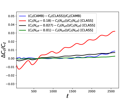
Figure 1: Relative variations of the predicted temperature spectra between CLASS and CAMB (blue). We also compare the spectra when we shift $N_{\mathrm{{eff}}}$  toward negative values for $\Delta N_{\mathrm{{eff}}}=-0.18$ (red), $\Delta N_{\mathrm{{eff}}}=-0.027$ (black) and $\Delta N_{\mathrm{{eff}}}=-0.01$ (green) with CLASS ($\theta$ is fixed, $H_{0}$ is therefore recalculated).

3 $\rm{TT}$+$\rm{TE}$+$\rm{EE}$+BAO results

In this section, we discuss the results obtained with the combination of Planck TT+TE+EE (so-called ALL) likelihoods together with BAO data. They are given in Table 2, and are classified according to various kind of systematic errors. Each of them is further discussed in a dedicated subsection below: we first assess the impact of the choice of the Boltzmann solver, then we discuss the impact of the choice of the high$-\ell$ likelihood. Finally we compare the results using different statistical analysis.

All the values which are tagged with a ${\sharp}$ are extracted from the PLA.

	Planck $\cal{L}$	Config	$N_{\mathrm{{eff}}}$
	+lowTEB+BAO
1	PlikALL♯	MCMC/CAMB	$3.04\pm 0.18$
	Boltzmann code and sampler systematics
2	PlikALL	MCMC/CLASS	$3.03^{-0.17}_{+0.17}$
	Likelihood systematics
3	CamSpecALL♯	MCMC/CAMB	$2.89\pm 0.19$
4	hlpALL(PS)	MCMC/CLASS	$2.92^{-0.15}_{+0.15}$
5	hlpALL	MCMC/CLASS	$2.86^{-0.14}_{+0.15}$
	Statistical analysis systematics
6	PlikALL	Profile/CLASS	$3.00_{-0.20}^{+0.19}$
7	hlpALL(PS)	Profile/CLASS	$2.87_{-0.14}^{+0.15}$
8	hlpALL	Profile/CLASS	$2.85\pm 0.14$
9	hlpALL(Plik-like)	Profile/CLASS	$2.90_{-0.16}^{+0.17}$

Table 2: Results on $N_{\mathrm{{eff}}}$ obtained when combining PlikALL, hlpALL(PS) and hlpALL with BAO(errors are given at 68$\%$CL). lowTEB has been used at low-$\ell$.

3.1 Boltzmann code and sampler effects

In this subsection, we study the impact of the choice of the Boltzmann solver that is used to infer cosmological parameters. Within our setup we cannot disentangle the impact of the Boltzmann code from the one of the sampler used for the MCMC mutiparameter space exploration, as a consequence the estimation given in this section combine both effects.

The comparison of the results using Plik are given in Table 2 (line 1 and 2): the use of CLASS combined with the CAMEL MCMC sampler tends to induce slightly smaller error bars on $N_{\mathrm{{eff}}}$ as well as a very small shift of $0.01$ toward lower values when results are compared with the public Planck results. It is further illustrated by the difference between the black (for the public/CAMB) and the blue (for this work/CLASS) marginal distributions on cosmological parameters shown on Fig. 2 (see next section for a full description of the Figure). This shift is consistent with the difference shown on Fig. 1 between spectra predicted by both Boltzmann solvers, and is largely subdominant compared to the statistical uncertainty.

We also tested the effect of changing the neutrino model. We have compared the results when attributing to each of the three neutrinos a mass derived from the Normal Hierarchy scenario expectation and found a $0.01$ shift of the $N_{\mathrm{{eff}}}$ results. Given the actual precisions on the CMB spectra, we can therefore safely assume a $\mathrm{\Lambda{CDM}}$ model with only one massive neutrino carrying all the mass.

3.2 Likelihood comparisons

3.2.1 Results

A possible source of systematic error to be estimated is the one related to the choice of the Planck high-$\ell$ likelihood. As discussed in Sect. 2.2, various assumptions have been made to build the likelihood. The comparison of the results from each likelihood allows to quantify the impact of the underlying assumptions.

A discrepancy between PlikALL and CamSpecALL is already mentioned in Planck Collaboration XIII (2016), which quotes $\Delta N_{\mathrm{{eff}}}\simeq 0.15$. Using the HiLLiPOP(PS) likelihoods, we find differences of the same order of magnitude as quoted in Table 2 (line 1 vs. lines 3,4,5). This variation can reach a maximum of $\Delta N_{\mathrm{{eff}}}\simeq 0.17$.

However, as stated in Sect. 2.2, there are more data in the HiLLiPOP likelihoods than in Plik and CamSpec. This can affect the interpretation of the shift, as part of it might be due to statistical fluctuations. To test this effect, we have derived the results using HiLLiPOP(PS) while removing the $100\times 143$, $100\times 217$ and two of the four $143\times 217$ cross-spectra, and reducing the $\ell$ range (cf. Sect. 2.2.2): the result is quoted on line 9 and labelled HiLLiPOP(Plik-like). We see that a small part (up to $0.03$) of those $0.17$ may be attributed to a statistical effect (including the covariance matrix determination).

3.2.2 Correlations with other parameters

In this section we investigate the correlation between $N_{\mathrm{{eff}}}$ and the cosmological and nuisance parameters, the definition of the lattest being given in Table A1. For hlpTT, the model for the point source residuals is slighly different (see Section 2.2.2): $A_{\hbox{radio}}$ and $A_{\hbox{dusty}}$ are respectively the amplitudes of the radio sources and the dusty galaxies (Couchot et al., 2017). The nuisance parameters for Plik are further defined in Planck Collaboration (2014) and Planck Collaboration XI (2016). The cosmological parameters we infer together with $N_{\mathrm{{eff}}}$ are the sixth parameters of the base $\mathrm{\Lambda{CDM}}$ model, as defined in Planck Collaboration XVI (2014), namely:

• $\Omega_{b}h^{2}$: Today’s baryon density

• $\Omega_{c}h^{2}$: Today’s cold dark matter density

• $H_{0}$: Current expansion rate in $\hbox{km.s}^{-1}\hbox{.Mpc}^{-1}$

• $\tau_{\rm reio}$: Optical depth to reionization

• $n_{s}$: Scalar spectrum power-law index

• $\ln(10^{10}A_{s})$: Log power of the primordial curvature perturbations

We give on Table 3 and Fig. 2 the results of the CAMEL MCMC sampler using the CLASS Boltzmann solver with PlikALL, hlpALL(PS) and hlpALL (combined with lowTEB and BAO) compared to the Planck public chains for $N_{\mathrm{{eff}}}$ plus the six $\mathrm{\Lambda{CDM}}$ parameters. Similarly to what is observed on $N_{\mathrm{{eff}}}$, we find variations of the parameters between likelihoods of the order of one sigma or less. The error bars of the HiLLiPOP likelihoods are slightly smaller due to the additional data that are used (cf. Sect. 2.2.2).

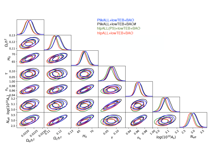
Figure 2: Cosmological parameters obtained with a combination of lowTEB, BAOand high$-\ell$ likelihoods: HiLLiPOP(PS), HiLLiPOP, Plik/CLASS and Plik/CAMB (the chains are the ones of the PLA using CAMB).

Param	hlpALL(PS)[CLASS]	hlpALL[CLASS]	PlikALL[CLASS]	PlikALL[CAMB]♯
$\Omega_{b}h^{2}$	$0.02215^{-0.00017}_{+0.00018}$	$0.02213^{-0.00018}_{+0.00017}$	$0.02227^{-0.00018}_{+0.00018}$	$0.02229^{-0.00019}_{+0.00019}$
$\Omega_{c}h^{2}$	$0.1163^{-0.0023}_{+0.0025}$	$0.1155^{-0.0023}_{+0.0023}$	$0.1187^{-0.0029}_{+0.0030}$	$0.1191^{-0.0031}_{+0.0030}$
$H_{0}$	$67.14^{-1.01}_{+1.074}$	$66.71^{-1.02}_{+1.058}$	$67.51^{-1.13}_{+1.125}$	$67.49^{-1.21}_{+1.235}$
$\tau_{\rm reio}$	$0.069^{-0.016}_{+0.016}$	$0.074^{-0.015}_{+0.014}$	$0.077^{-0.016}_{+0.016}$	$0.082^{-0.017}_{+0.017}$
$n_{s}$	$0.961^{-0.006}_{+0.006}$	$0.962^{-0.006}_{+0.006}$	$0.965^{-0.007}_{+0.007}$	$0.966^{-0.008}_{+0.008}$
$\ln(10^{10}A_{s})$	$3.06^{-0.03}_{+0.03}$	$3.07^{-0.03}_{+0.03}$	$3.09^{-0.03}_{+0.03}$	$3.10^{-0.04}_{+0.03}$
$N_{\mathrm{{eff}}}$	$2.92^{-0.15}_{+0.15}$	$2.86^{-0.14}_{+0.15}$	$3.03^{-0.17}_{+0.17}$	$3.04^{-0.18}_{+0.18}$

Table 3: Results on MCMC chains for all cosmological parameters obtained when combining the PlikALL, hlpALL(PS) and hlpALL  Planck likelihoods with lowTEB and BAO (errors are given at 68$\%$CL).

The correlations between $N_{\mathrm{{eff}}}$ and the nuisance parameters are illustrated on Fig. 3 for the three likelihoods (from top to bottom: hlpALL(PS), hlpALL, PlikALL). For HiLLiPOP(PS), the highest values of the coefficients are obtained for the nuisance parameters related to foregrounds which play a role at small scales: namely the point sources (with a “PS” label in the name of the parameter) and/or the SZ sector. $N_{\mathrm{{eff}}}$ is anti-correlated to the point source parameters when the related nuisance parameters are left free to vary (as this is the case of HiLLiPOP). While, adding information in the point source model (as done in HiLLiPOP), this relation is broken. We also observe a correlation between $N_{\mathrm{{eff}}}$ and $A_{\rm{kSZ}}$ (the amplitude of the kinetic SZ effect) and $A_{\rm{SZxCIB}}$ (the amplitude of the correlation between SZ and the Cosmic Infrared Background CIB) but those parameters are only very slightly constrained with Planck data. For Plik, the correlation level is lower for all nuisance parameters, but the number of parameters is higher.

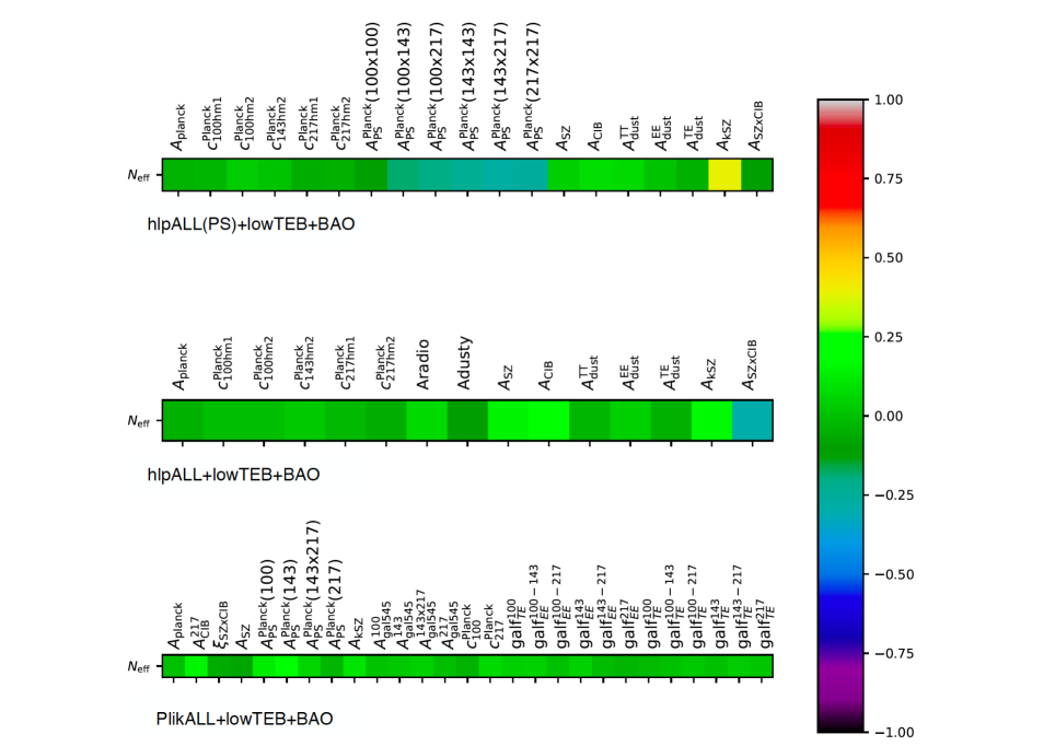
Figure 3: Correlation coefficients between $N_{\mathrm{{eff}}}$ and the nuisance parameters from top to bottom for hlpALL(PS), hlpALL and PlikALL when combined with BAO and lowTEB.

3.3 Statistical analysis systematics

3.3.1 Results

In this section, we sudy the impact of the choice of the statistical analysis (Bayesian vs. frequentist). The main purpose of such a comparison is to check for any volume effect that may impact significantly the results (see for example Hamann, 2012). The $N_{\mathrm{{eff}}}$ estimates for various Planck likelihoods using profile likelihoods are given on lines 6 to 8 of Table 2. A visual comparison of the results are shown on Fig. 4, where the profile analysis results are transformed in terms of ${\cal{L}/\cal{L}}_{max}$ and are superimposed to the MCMC posterior distributions.

The profile analysis results systematically lead to smaller mean values, keeping the error bars almost similar. This effect is also present in the PLA: for example, the $N_{\mathrm{{eff}}}$ values extracted from the best fit procedure (which is exactly what is done in a profile analysis) quoted for the PlikALL+lowTEB+BAO combination is equal to $2.996$, a value which is $\simeq 0.04$ smaller than the maximum of the MCMC posterior distributions. The variation is specific to each likelihood and not expected to be constant as it reflects its very shape in the multidimensional parameter space. The higher volume effect is observed for HiLLiPOP(PS) and does not exceed $\Delta N_{\mathrm{{eff}}}=0.05$.

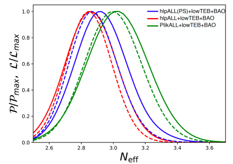
Figure 4: Posterior distributions of the MCMC analysis (plain lines) and Profile likelihood ratio ${\cal{L}/\cal{L}}_{max}$ (dashed lines) for hlpALL(PS) (blue), hlpALL (red), and PlikALL (green) combined with lowTEB+BAO.

3.3.2 Statistical and Nuisance error contribution

Following the procedure described in Aad et al. (2014), we have separately estimated the two contributions to the total error: the one coming from statistics and the one linked to the foreground and instrumental modelling (so-called nuisance error). We first built the usual profiles for each likelihood: they are shown in solid lines on Fig. 5 and the corresponding results are given in lines 6 to 8 of Table 2. In a second step, we built another set of profiles, fixing the nuisance parameters to the values of the previously obtained best-fit. The errors derived from this second fit (shown in dashed line on Fig. 5) correspond to the ultimate error one would obtain if we knew the nuisance parameters perfectly (and they had the values given by the best-fit). Finally the nuisance error of each individual likelihood is deduced by quadratically subtracting the statistical uncertainty from the total error. The results are given in Table 4.

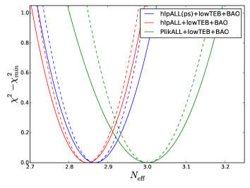
Figure 5: Comparison of profile likelihoods obtained for the combination of hlpALL(PS) (blue), hlpALL (red) and PlikALL (green) together with BAO and lowTEB. The superimposed dashed profiles have been obtained when fixing the nuisance parameters values to the ones obtained for the best fit of each likelihood combination.

Planck $\cal{L}$	Mean	Full	Stat	Nuisance
lowTEB+BAO	Value	Error	Error	Error
PlikALL	$3.00$	${}_{-0.20}^{+0.19}$	${}_{-0.15}^{+0.16}$	${}_{-0.13}^{+0.12}$
hlpALL(PS)	$2.87$	${}_{-0.14}^{+0.15}$	$\pm 0.13$	${}_{-0.05}^{+0.06}$
hlpALL	$2.85$	$\pm 0.14$	$\pm 0.13$	${}_{-0.05}^{+0.05}$
hlpALL(Plik-like)	$2.90$	${}_{-0.16}^{+0.17}$	${}_{-0.15}^{+0.16}$	${}_{-0.05}^{+0.05}$

Table 4: Full error on $N_{\mathrm{{eff}}}$ and contributions from Statistics and Nuisance derived using profile likelihoods and CLASS (cf. description of the procedure in Section 3.3.2) obtained when combining PlikALL, hlpALL(PS) and hlpALL with lowTEB and BAO.

From the comparison of the results of hlpALL(Plik-like) and hlpALL(PS), we can deduce that the additionnal data induce a slight shift ($\Delta N_{\mathrm{{eff}}}=0.03$), apart from the expected reduction of the statistical error.

From the comparison of the results of hlpALL(Plik-like) and PlikALL, we observe that the statistical error is exactly the same: giving high confidence to the fact that the impact of the different choices made in the likelihood implementation for the covariance matrix is negligible. The remaining difference, which happens to be the bigger one, comes from the effect of the foreground modelling, which impacts both the mean value and the nuisance error. The foreground modelling (but a different one) is also tested through the comparison of the results of hlpALL(PS) and hlpALL.

3.4 Other cosmological data

We have further tested the impact of CMB Lensing on the $N_{\mathrm{{eff}}}$ measurement and found it to be very small, as expected (cf. Planck Collaboration XIII, 2016), slightly lowering the overall results by $0.01$.

We have also checked that the choice of the low-$\ell$ likelihood had no impact on the final results (replacing lowTEB with Lollipop+Commander as stated in Sect. 2.2.1).

It has to be noted that the supernovae data do not help to further constraint $N_{\mathrm{{eff}}}$ once the BAO data are used, we therefore chose not to use them in this analysis. For completeness we note that the update of the BAO data from DR11 to DR12 does not impact the constraint on $N_{\mathrm{{eff}}}$ (Alam et al., 2017).

3.5 Summary

The results on $N_{\mathrm{{eff}}}$ are summarized in Fig. 6. The shift of the mean values observed when using a likelihood or another is of the same order of magnitude as the error derived from each individual likelihood ($\Delta N_{\mathrm{{eff}}}\simeq 0.17$ vs. $\sigma(N_{\mathrm{{eff}}})=0.18$). It has been shown to be mainly driven by the assumptions made for the foreground modelling. A small part of this variation (up to $0.03$) has been identified to be linked to the data considered in HiLLiPOP(PS) and not in Plik. Still, it is high enough not to be neglected when constraining theoretical models from the $N_{\mathrm{{eff}}}$ measurement only.

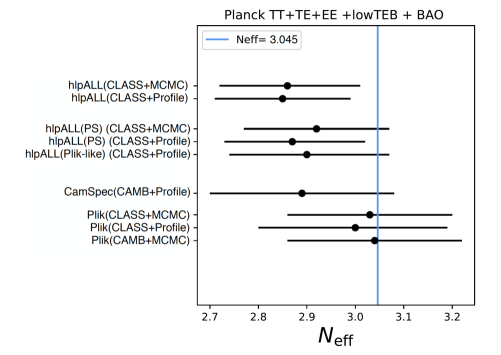
Figure 6: Results comparisons for the combination of Planck $\rm{TT}$+$\rm{TE}$+$\rm{EE}$ likelihoods, with lowTEB and BAO.

4 Fitting $\rm{TT}$ and $\rm{TE}$ separately

In the previous sections we have shown the results of the combination of temperature and polarisation CMB data. In the following, we estimate $N_{\mathrm{{eff}}}$ for $\rm{TT}$ and $\rm{TE}$ separately to further compare the outcome of each likelihood.

4.1 $\rm{TT}$+lowTEB+BAO results

In this section, we consider the combination of temperature-only CMB likelihoods, together with BAO data. The results are summarized in Table 5 for various configurations. For this specific combination the CamSpec results are not public, we therefore cannot use them in the comparison.

Planck $\cal{L}$	Config	$N_{\mathrm{{eff}}}$
+lowTEB+BAO
PlikTT♯	MCMC/CAMB	$3.15\pm 0.23$
PlikTT	Profile/CLASS	$3.09_{-0.22}^{+0.21}$
hlpTT(PS)	Profile/CLASS	$3.27_{-0.26}^{+0.28}$
hlpTT	Profile/CLASS	$3.20_{-0.20}^{+0.21}$

Table 5: Results on $N_{\mathrm{{eff}}}$ obtained when combining PlikTT, hlpTT(PS) and hlpTT with BAO (errors are given at 68$\%$CL). lowTEB has been used at low-$\ell$.

From this Table, we obtain $\Delta N_{\mathrm{{eff}}}\simeq 0.18$ from the largest difference observed between hlpTT(PS)-Profile/CLASS and PlikTT^♯-Profile/CLASS.

As in the previous section, we have checked that the impact of the neutrino settings is almost negligible, as well as the impact of supernovae data. In addition, the choice of the DR12 BAO data instead of DR11 has no effect.

4.2 $\rm{TE}$+lowTEB+BAO results

Given the Planck noise level, the $\rm{TE}$ likelihoods lead to similar results than those obtained with $\rm{TT}$ on $\mathrm{\Lambda{CDM}}$. In addition they are less sensitive to the foreground modellings (Galli et al., 2014; Couchot et al., 2017b). In this section we use of the $\rm{TE}$ likelihood in place of the $\rm{TT}$ one and compare the results obtained on $N_{\mathrm{{eff}}}$ when combined with lowTEB and BAO on Table 6.

The remaining $\Delta N_{\mathrm{{eff}}}$ is of the order of 0.07, which is small with respect to the total error with $\rm{TE}$ only. It may still contain some residual systematics from temperature to polarisation leakage which study is beyond the scope of this paper.

Planck $\cal{L}$	Config	lowTEB
PlikTE	MCMC/CAMB	$2.94\pm 0.37$
hlpTE	Profile/CLASS	$3.01_{-0.30}^{+0.32}$

Table 6: Results on $N_{\mathrm{{eff}}}$ obtained when combining BAO with PlikTE, and hlpTE (errors are given at 68$\%$CL). lowTEB has been used at low-$\ell$.

5 Conclusions

We have studied in detail the estimation of the effective number of relativistic species from CMB Planck data. We have tested different ingredients of the analysis to further quantify their impact on the results: mainly the Boltzmann codes, the high$-\ell$ likelihoods (Plik, HiLLiPOP and CamSpec), and the statistical analysis.

• The estimated variation of $N_{\mathrm{{eff}}}$ when switching from CAMB to CLASS is negligible, of the order of $\Delta N_{\mathrm{{eff}}}=0.01$.

• If we can safely neglect the impact of the covariance matrix estimation, as suggested by the obtained results, the variation linked to the assumptions on foreground residuals modelling derived from the comparison of the high$-\ell$ likelihoods has been estimated to be of the order of $\Delta N_{\mathrm{{eff}}}=0.17$ on which a small part (up to $0.03$) may be attributed to a statistical effect. We have also shown that, at least for HiLLiPOP(PS), $N_{\mathrm{{eff}}}$ was mainly correlated with nuisance parameters linked to foregrounds playing a role at small scales (ie. point sources and SZ).

• We have found slight differences between the Bayesian and the frequentist inferred mean values, linked to particular likelihood volume effects. A shift between both methods has been estimated to be $\Delta N_{\mathrm{{eff}}}\leq 0.05$.

As an overall conclusion, we have shown that the variation of the mean $N_{\mathrm{{eff}}}$ values is non-negligible. This foreground related systematic uncertainty is of the same order of magnitude as the error derived for each individual likelihood. In addition the results obtained with HiLLiPOP(PS) and CamSpec lead systematically to lower values than the ones derived from the public Planck likelihood.

We have cross-checked the consistency of the results when considering $\rm{TT}$ and $\rm{TE}$ separately. When considering $\rm{TE}$ only (together with BAO and lowTEB), which is less sensitive to foreground residuals, this observed variation drops down to $\Delta N_{\mathrm{{eff}}}=0.05$ for the likelihoods we have been able to compare.

We have shown that likelihood modelling is an important challenge for the current Planck measurements for the $N_{\mathrm{{eff}}}$ interpretation, even for temperature data. The shift discussed in this paper is very large compared to the $\sigma(N_{\mathrm{{eff}}})=0.027$ statistical-only expectations for CMB-S4. We however expect data from the next generation of CMB experiments to be more robust to such systematic error. The increase in constraining power from the $\rm{TE}$ power spectrum with respect to the $\rm{TT}$ one, as well as the better determination of the temperature power spectrum on small scales will reduce the impact of foregrounds mismodelling.

Appendix on nuisance parameters

This appendix presents the nuisance parameters of the HiLLiPOP likelihood in table A1.

name	definition
Instrumental calibrations
$c^{\textsc{Planck}}_{100hm1}$	map calibration (100-hm1)
$c^{\textsc{Planck}}_{100hm2}$	map calibration (100-hm2)
$c^{\textsc{Planck}}_{143hm1}$	map calibration (143-hm1)
$c^{\textsc{Planck}}_{143hm2}$	map calibration (143-hm2)
$c^{\textsc{Planck}}_{217hm1}$	map calibration (217-hm1)
$c^{\textsc{Planck}}_{217hm2}$	map calibration (217-hm2)
$A_{\textsc{Planck}}$	absolute calibration
Foreground modellings
$A^{\textsc{Planck}}_{\rm PS}(100\times 100)$	PS amplitude in TT (100x100 GHz)
$A^{\textsc{Planck}}_{\rm PS}(100\times 143)$	PS amplitude in TT (100x143 GHz)
$A^{\textsc{Planck}}_{\rm PS}(100\times 217)$	PS amplitude in TT (100x217 GHz)
$A^{\textsc{Planck}}_{\rm PS}(143\times 143)$	PS amplitude in TT (143x143 GHz)
$A^{\textsc{Planck}}_{\rm PS}(143\times 217)$	PS amplitude in TT (143x217 GHz)
$A^{\textsc{Planck}}_{\rm PS}(217\times 217)$	PS amplitude in TT (217x217 GHz)
$A_{\rm radio}$	scaling for radio sources (TT)
$A_{\rm dusty}$	scaling for infrared sources (TT)
$A_{\rm SZ}$	scaling for the tSZ template (TT)
$A_{\rm CIB}$	scaling for the CIB template (TT)
$A_{\rm kSZ}$	scaling for the kSZ template (TT)
$A_{\rm SZxCIB}$	scaling for kSZ x CIB cross correlation
$A_{\rm dust}^{\rm TT}$	scaling for the dust in TT
$A_{\rm dust}^{\rm EE}$	scaling for the dust in EE
$A_{\rm dust}^{\rm TE}$	scaling for the dust in TE

Table A1: Nuisance parameters for the HiLLiPOP likelihood.

References

- Aad et al. (2014) Aad, G. et al., Measurement of the Higgs boson mass from the and channels with the ATLAS detector using 25 fb-1 of collision data. 2014, Phys. Rev., D90, 052004, 1406.3827
- Abazajian et al. (2015) Abazajian, K. N. et al., Neutrino Physics from the Cosmic Microwave Background and Large Scale Structure. 2015, Astropart. Phys., 63, 66, 1309.5383
- Abazajian et al. (2016) Abazajian, K. N. et al., CMB-S4 Science Book, First Edition. 2016, 1610.02743
- Alam et al. (2017) Alam, S. et al., The clustering of galaxies in the completed SDSS-III Baryon Oscillation Spectroscopic Survey: cosmological analysis of the DR12 galaxy sample. 2017, Mon. Not. Roy. Astron. Soc., 470, 2617, 1607.03155
- Beringer et al. (2012) Beringer, J. et al., Review of Particle Physics (RPP). 2012, Phys.Rev., D86, 010001
- Beutler et al. (2014) Beutler, F. et al., The clustering of galaxies in the SDSS-III Baryon Oscillation Spectroscopic Survey: Signs of neutrino mass in current cosmological datasets. 2014, Mon.Not.Roy.Astron.Soc., 444, 3501, 1403.4599
- Binetruy et al. (2000) Binetruy, P., Deffayet, C., Ellwanger, U., & Langlois, D., Brane cosmological evolution in a bulk with cosmological constant. 2000, Phys.Lett., B477, 285, hep-th/9910219
- Bird et al. (2012) Bird, S., Viel, M., & Haehnelt, M. G., Massive neutrinos and the non-linear matter power spectrum. 2012, MNRAS, 420, 2551, 1109.4416
- Blas et al. (2011) Blas, D., Lesgourgues, J., & Tram, T., The Cosmic Linear Anisotropy Solving System (CLASS). Part II: Approximation schemes. 2011, J. Cosmology Astropart. Phys., 7, 034, 1104.2933
- Blennow et al. (2012) Blennow, M., Fernandez-Martinez, E., Mena, O., Redondo, J., & Serra, P., Asymmetric Dark Matter and Dark Radiation. 2012, JCAP, 1207, 022, 1203.5803
- Calabrese et al. (2011) Calabrese, E., Huterer, D., Linder, E. V., Melchiorri, A., & Pagano, L., Limits on Dark Radiation, Early Dark Energy, and Relativistic Degrees of Freedom. 2011, Phys.Rev., D83, 123504, 1103.4132
- Calabrese et al. (2008) Calabrese, E., Slosar, A., Melchiorri, A., Smoot, G. F., & Zahn, O., Cosmic Microwave Weak lensing data as a test for the dark universe. 2008, Phys. Rev., D77, 123531, 0803.2309
- Caramete & Popa (2014) Caramete, A. & Popa, L., Cosmological evidence for leptonic asymmetry after Planck. 2014, JCAP, 1402, 012, 1311.3856
- Consiglio et al. (2018) Consiglio, R., de Salas, P. F., Mangano, G., et al., PArthENoPE reloaded. 2018, Comput. Phys. Commun., 233, 237, 1712.04378
- Couchot et al. (2017a) Couchot, F., Henrot-Versillé, S., Perdereau, O., et al., Cosmological constraints on the neutrino mass including systematic uncertainties. 2017a, Astron. Astrophys., 606, A104, 1703.10829
- Couchot et al. (2017b) Couchot, F., Henrot-Versillé, S., Perdereau, O., et al., Cosmology with the cosmic microwave background temperature-polarization correlation. 2017b, Astron. Astrophys., 602, A41, 1609.09730
- Couchot et al. (2017) Couchot, F., Henrot-Versillé, S., Perdereau, O., et al., Cosmology with the cosmic microwave background temperature-polarization correlation. 2017, A&A, 602, A41, 1609.09730
- Couchot et al. (2017) Couchot, F., Henrot-Versillé, S., Perdereau, O., et al., Relieving tensions related to the lensing of the cosmic microwave background temperature power spectra. 2017, Astron. Astrophys., 597, A126, 1510.07600
- de Salas & Pastor (2016) de Salas, P. F. & Pastor, S., Relic neutrino decoupling with flavour oscillations revisited. 2016, J. Cosmology Astropart. Phys., 7, 051, 1606.06986
- Fischler & Meyers (2011) Fischler, W. & Meyers, J., Dark Radiation Emerging After Big Bang Nucleosynthesis? 2011, Phys.Rev., D83, 063520, 1011.3501
- Flambaum & Shuryak (2006) Flambaum, V. & Shuryak, E., Possible evidence for ’dark radiation’ from big bang nucleosynthesis data. 2006, Europhys.Lett., 74, 813, hep-th/0512038
- Galli et al. (2014) Galli, S., Benabed, K., Bouchet, F., et al., CMB polarization can constrain cosmology better than CMB temperature. 2014, Phys. Rev. D, 90, 063504, 1403.5271
- Haario et al. (2001) Haario, H., Saksman, E., & Tamminen, J., An adaptive Metropolis algorithm. 2001, Bernoulli, 7, 223
- Hamann (2012) Hamann, J., Evidence for extra radiation? Profile likelihood versus Bayesian posterior. 2012, J. Cosmology Astropart. Phys., 3, 021, 1110.4271
- Hamann et al. (2010) Hamann, J., Hannestad, S., Raffelt, G. G., Tamborra, I., & Wong, Y. Y. Y., Cosmology seeking friendship with sterile neutrinos. 2010, Phys. Rev. Lett., 105, 181301, 1006.5276
- Hannestad et al. (2010) Hannestad, S., Mirizzi, A., Raffelt, G. G., & Wong, Y. Y., Neutrino and axion hot dark matter bounds after WMAP-7. 2010, JCAP, 1008, 001, 1004.0695
- Henrot-Versillé et al. (2016) Henrot-Versillé, S., Perdereau, O., Plaszczynski, S., et al., Agnostic cosmology in the CAMEL framework. 2016, 1607.02964
- Henrot-Versillé et al. (2015) Henrot-Versillé, S. et al., Improved constraint on the primordial gravitational-wave density using recent cosmological data and its impact on cosmic string models. 2015, Class. Quant. Grav., 32, 045003, 1408.5299
- Lesgourgues (2011) Lesgourgues, J., The Cosmic Linear Anisotropy Solving System (CLASS) III: Comparision with CAMB for LambdaCDM. 2011, ArXiv e-prints, 1104.2934
- Lewis et al. (2000) Lewis, A., Challinor, A., & Lasenby, A., Efficient Computation of Cosmic Microwave Background Anisotropies in Closed Friedmann-Robertson-Walker Models. 2000, ApJ, 538, 473, arXiv:astro-ph/9911177
- Mangilli et al. (2015) Mangilli, A., Plaszczynski, S., & Tristram, M., Large-scale cosmic microwave background temperature and polarization cross-spectra likelihoods. 2015, MNRAS, 453, 3174, 1503.01347
- Melchiorri et al. (2007) Melchiorri, A., Mena, O., & Slosar, A., An improved cosmological bound on the thermal axion mass. 2007, Phys.Rev., D76, 041303, 0705.2695
- Planck Collaboration (2014) Planck Collaboration, Planck 2013 results. XV. CMB power spectra and likelihood. 2014, A&A, 571, A15, 1303.5075
- Planck Collaboration XVI (2014) Planck Collaboration XVI, Planck 2013 results. XVI. Cosmological parameters. 2014, A&A, 571, A16, 1303.5076
- Planck Collaboration XI (2016) Planck Collaboration XI, Planck 2015 results. XI. CMB power spectra, likelihoods, and robustness of parameters. 2016, A&A, 594, A11, 1507.02704
- Planck Collaboration XIII (2016) Planck Collaboration XIII, Planck 2015 results. XIII. Cosmological parameters. 2016, A&A, 594, A13, 1502.01589
- Planck Collaboration Int. XXII (2015) Planck Collaboration Int. XXII, Planck intermediate results. XXII. Frequency dependence of thermal emission from Galactic dust in intensity and polarization. 2015, A&A, submitted, 576, A107, 1405.0874
- Planck Collaboration Int. XXX (2016) Planck Collaboration Int. XXX, Planck intermediate results. XXX. The angular power spectrum of polarized dust emission at intermediate and high Galactic latitudes. 2016, A&A, 586, A133, 1409.5738
- Planck Collaboration Int. XLVII (2016) Planck Collaboration Int. XLVII, Planck intermediate results. XLVII. Constraints on reionization history. 2016, A&A, 596, A108, 1605.03507
- Shiromizu et al. (2000) Shiromizu, T., Maeda, K.-i., & Sasaki, M., The Einstein equation on the 3-brane world. 2000, Phys.Rev., D62, 024012, gr-qc/9910076
- Smith et al. (2006) Smith, T. L., Pierpaoli, E., & Kamionkowski, M., A new cosmic microwave background constraint to primordial gravitational waves. 2006, Phys.Rev.Lett., 97, 021301, astro-ph/0603144
- Takahashi et al. (2012) Takahashi, R., Sato, M., Nishimichi, T., Taruya, A., & Oguri, M., Revising the Halofit Model for the Nonlinear Matter Power Spectrum. 2012, ApJ, 761, 152, 1208.2701
- Tanabashi et al. (2018) Tanabashi, M., Hagiwara, K., Hikasa, K., et al., Review of Particle Physics. 2018, Phys. Rev. D, 98, 030001
- Tristram et al. (2005) Tristram, M., Macías-Pérez, J. F., Renault, C., & Santos, D., XSPECT, estimation of the angular power spectrum by computing cross-power spectra with analytical error bars. 2005, MNRAS, 358, 833, arXiv:astro-ph/0405575