A critical strange metal from fluctuating gauge fields in a solvable random model

Abstract

Building upon techniques employed in the construction of the Sachdev-Ye-Kitaev (SYK) model, which is a solvable $0+1$ dimensional model of a non-Fermi liquid, we develop a solvable, infinite-ranged random-hopping model of fermions coupled to fluctuating U(1) gauge fields. In a specific large-$N$ limit, our model realizes a gapless non-Fermi liquid phase, which combines the effects of hopping and interaction terms. We derive the thermodynamic properties of the non-Fermi liquid phase realized by this model, and the charge transport properties of an infinite-dimensional version with spatial structure.

I Introduction

A number of models of strange metals have been been constructed Parcollet and Georges (1999); Gu et al. (2017, 2017); Davison et al. (2017); Song et al. (2017); Zhang (2017); Haldar et al. (2018); Ben-Zion and McGreevy (2018); Patel et al. (2018a); Chowdhury et al. (2018); Fu et al. (2018) by connecting together ‘quantum islands’, in which each island has random all-to-all interactions between the electrons i.e. each island is a 0+1 dimensional SYK model Sachdev and Ye (1993); Kitaev (2015); Sachdev (2015); Kitaev and Suh (2018). Some of these models Parcollet and Georges (1999); Song et al. (2017); Patel et al. (2018a); Chowdhury et al. (2018) exhibit ‘bad metal’ behavior above some crossover temperature, with a resistivity which increases linearly with temperature ($T$), and has a magnitude (in two dimensions) which is larger than the quantum unit of resistance $h/e^{2}$. These models can be useful starting points for understanding a variety of experiments above moderate values of $T$, and they also predict Sachdev and Ye (1993); Parcollet and Georges (1999) the frequency independent density fluctuation spectrum observed in recent electron scattering experiments Mitrano et al. (2018). However, some of the most interesting and puzzling observations exhibit Cooper et al. (2009); Jin et al. (2011); Legros et al. (2018) linear-in-$T$ resistivity down to vanishingly small $T$, with a resistivity which is much smaller than $h/e^{2}$. Kondo-like two-band SYK models have been proposed for such behavior Patel et al. (2018a); Chowdhury et al. (2018), in which a band of itinerant electrons acquires marginal-Fermi liquid behavior Varma et al. (1989) upon Kondo exchange scattering off localized electrons in SYK islands. The holographic models of strange metals have a structure very similar to these Kondo-SYK models Faulkner et al. (2013); Cubrovic et al. (2009); Sachdev (2010).

A possible shortcoming of the two-band SYK-Kondo models Patel et al. (2018a); Chowdhury et al. (2018) is that density of itinerant carriers is ‘small’. In other words, only the itinerant electrons carry current and exhibit marginal-Fermi liquid behavior, while the localized electrons in SYK islands only act as a background ‘bath’ of incoherent electrons which dissipates current from the itinerant electrons. This behavior does not appear to be in accord with estimates of the magnitude of the linear-in-$T$ resistivity as $T\rightarrow 0$ Legros et al. (2018).

In this paper, we shall propose and solve a SYK-like model which exhibits strange metal resistivity as $T\rightarrow 0$, and in which the density of itinerant fermions is ‘large’. We shall examine a model of fermions coupled to an emergent, dynamic, U(1) gauge field. We shall show that a solvable SYK-like large $N$ limit exists, in which the electrons are in $N$ clusters with $M$ sites per cluster ($M/N$ is fixed as the large $N$ limit is taken): see Fig. 1.

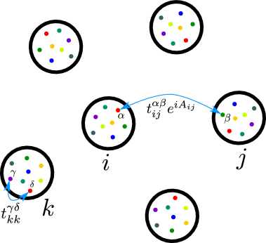
Figure 1: A cartoon of our model. It consists of $N$ clusters indexed by $i,j,...$, each of which contains $M$ sites indexed by $\alpha,\beta,...$. Random hopping occurs between all possible pairs of intra-cluster and inter-cluster sites, but only inter-cluster hops are coupled to dynamic U(1) gauge fields $A_{ij}$. The model is solved in the $M,N\rightarrow\infty$ limit, with $M/N$ fixed.

The DC conductivity of our model is presented in Eq. (49), and the resistivity varies as $T^{2x}$ as $T\rightarrow 0$, with the exponent $x$ dependent only upon $M/N$ and the particle-hole asymmetry parameter $\mathcal{E}$, as shown in Eq. (23) and Fig. 3. In the limit of small $M/N$, $2x\sim 1$ (see Fig. 3), and then we have nearly linear-in-$T$ resistivity.

The problem of a finite density of fermions coupled to an emergent gauge field appears in many different physical contexts. The most extensively studied case is that related to compressible quantum Hall states in a half-filled Landau level Halperin et al. (1993). These studies begin with assumption that the fermions form a Fermi surface, and Landau damping from the fermions leads to an overdamped gauge propagator. The effects of the gauge coupling and the disorder are then treated perturbatively. The presence of disorder has a relatively modest effect in inducing a diffusive form for the gauge propagator. In the present paper we shall take a random all-to-all form of the fermion propagator, and show that this allows for an exact treatment of the gauge fluctuations. The local criticality exhibited by our model is expected to eventually crossover at low enough $T$ to more generic finite-dimensional behavior, but there is no theory yet for such a fixed point with strong disorder and interactions.

The physical context most appropriate for our proposed connection to observations on the overdoped cuprates Cooper et al. (2009); Legros et al. (2018) is the theory of an ‘algebraic charge liquid’ (ACL) Kaul et al. (2008) of spinless fermionic chargons coupled to an emergent gauge field. Specifically, in a SU(2) gauge theory of optimal doping quantum criticality Sachdev et al. (2009); Chowdhury and Sachdev (2015); Sachdev and Chowdhury (2016); Scheurer et al. (2018), it has been proposed that there could be an overdoped phase with a large density of fermionic chargons coupled to a deconfined SU(2) gauge field. For simplicity, this paper will consider the U(1) gauge field case, although the properties of the SU(2) case are expected to be very similar.

We will begin in Section II by defining the model and computing its saddle point equations in the large $N$ limit. The properties of the single fermion Green’s function as a function of frequency, temperature, and chemical potential will be described in Section III. The thermodynamics will be described in Section IV, and we will describe a higher-dimensional generalization which allows us to compute transport properties in Section V.

Appendix A describes an extension of our model in which the condensation of a charge 2 Higgs field leads to a metallic phase in which the fermions carry $\mathbb{Z}_{2}$ gauge charges. The Higgs condensate quenches the gauge field fluctuations, and the transport is therefore Fermi-liquid like. The Higgs condensate also reduces the density of low-energy fermionic excitations, and so we may view this transition as a model Sachdev et al. (2009); Chowdhury and Sachdev (2015); Sachdev and Chowdhury (2016); Scheurer et al. (2018) of optimal doping criticality from the overdoped side (no Higgs condensate) to the underdoped side (Higgs condensate present).

II Model and large-$N$ limit

We study a model of $N$ clusters, each with $M$ flavors of fermions, with infinite-ranged random hopping between the clusters that is coupled to fluctuating U(1) gauge fields. It is given by

$$\mathcal{H}=-\frac{1}{(MN)^{1/2}}\sum_{ij=1}^{N}\sum_{\alpha\beta=1}^{M}\left[t_{ij}^{\alpha\beta}e^{iA_{ij}}f^{\dagger}_{i\alpha}f_{j\beta}+(MN)^{1/2}\mu\delta_{ij}^{\alpha\beta}f^{\dagger}_{i\alpha}f_{i\alpha}\right],~{}~{}\ll t_{ij}^{\alpha\beta}t_{ji}^{\beta\alpha}\gg=\ll|t_{ij}^{\alpha\beta}|^{2}\gg=t^{2},~{}~{}A_{ji}=-A_{ij}.$$ (1)

where $N,M\rightarrow\infty$ and $M/N$ is an $\mathcal{O}(1)$ quantity. The $t_{ij}^{\alpha\beta}$ are complex gaussian random variables and $\ll..\gg$ denotes disorder-averaging; all disorder averages other than the ones explicitly shown above are zero. The clusters are indexed by $i$, and the sites (flavors) within a cluster, are indexed by $\alpha$. A cartoon of our model is shown in Fig. 1.

As in the analysis of the SYK models Sachdev (2015); Davison et al. (2017), we average over realizations of disorder. Doing so formally requires introducing replicas; however we assume, like in the SYK models, that there is no replica-symmetry breaking, restricting to replica-diagonal configurations and suppressing the then trivial sum over replicas. We introduce bilocal (in time) fields $G$ and $\Sigma$, obtaining the Euclidean action

$$S=\int d\tau\sum_{i=1}^{N}\sum_{\alpha=1}^{M}f^{\dagger}_{i\alpha}(\tau)(\partial_{\tau}+iA^{0}_{i}(\tau)+\mu)f_{i\alpha}(\tau)+t^{2}\frac{M}{N}\int d\tau d\tau^{\prime}\sum_{ij=1,i\leq j}^{N}e^{i(A_{ij}(\tau)-A_{ij}(\tau^{\prime}))}G_{j}(\tau-\tau^{\prime})G_{i}(\tau^{\prime}-\tau)$$

$$-M\int d\tau d\tau^{\prime}\sum_{i=1}^{N}\Sigma_{i}(\tau-\tau^{\prime})\left[G_{i}(\tau^{\prime}-\tau)-\frac{1}{M}\sum_{\alpha=1}^{M}f_{i\alpha}(\tau^{\prime})f^{\dagger}_{i\alpha}(\tau)\right].$$ (2)

The partition function is given by $Z=\int\mathcal{D}f\mathcal{D}f^{\dagger}\mathcal{D}A\mathcal{D}G\mathcal{D}\Sigma~{}e^{-S}$, and $\tau$ denotes Euclidean time. Unbounded integrals denote integration over the full range of the pertinent variable. Integrating out the Lagrange multipliers $\Sigma_{i}$ followed by the $G_{i}$ restores the pure disorder-averaged action. In the $M\rightarrow\infty$ limit, the integrals over the $\Sigma_{i}$ enforce the definitions of $G_{i}$ on each cluster $i$. The disorder averaged action is gauge-invariant under the transformations

$$A_{ij}(\tau)\rightarrow A_{ij}(\tau)+\theta_{i}(\tau)-\theta_{j}(\tau),~{}~{}f_{i\alpha}(\tau)\rightarrow f_{i\alpha}(\tau)e^{i\theta_{i}(\tau)},~{}~{}A^{0}_{i}(\tau)\rightarrow A^{0}_{i}(\tau)-\partial_{\tau}\theta_{i}(\tau),$$ (3)

with $G_{i}(\tau-\tau^{\prime})\rightarrow G_{i}(\tau-\tau^{\prime})e^{i(\theta_{i}(\tau)-\theta_{i}(\tau^{\prime}))}$ and $\Sigma_{i}(\tau-\tau^{\prime})\rightarrow\Sigma_{i}(\tau-\tau^{\prime})e^{i(\theta_{i}(\tau)-\theta_{i}(\tau^{\prime}))}$. The propagators of the scalar potentials $A^{0}_{i}$ will be screened due to the finite density of fermions Kim et al. (1994); fluctuations of the $A^{0}_{i}$ will be hence unable to inflict any singular self energy on the fermions at low energies, and we will thus simply ignore the $A^{0}_{i}$.

Examining the disorder-averaged action, after integrating out the fermions, does not immediately suggest a large-$N$ saddle-point for the $G_{i}$, but a simple large $N$ limit does turn out to exist. The reason is that there are enough ($M$) sites per cluster to self-average the cluster Green’s function $G_{i}$, so that the solution will have $G_{i}$ that don’t depend on $i$, even though there are $N$ clusters. This can be seen easily when the coupling to the gauge fields is turned off. Then we know the standard result for the fully-averaged Green’s function $G_{\mathrm{avg}}$ of the full large-$MN$ random matrix exactly, but can also express it as

$$G_{\mathrm{avg}}(\tau-\tau^{\prime})=\frac{1}{MN}\sum_{i=1}^{N}\sum_{\alpha=1}^{M}\langle f_{i\alpha}(\tau)f^{\dagger}_{i\alpha}(\tau^{\prime})\rangle=\frac{1}{N}\sum_{i}G_{i}(\tau-\tau^{\prime}).$$ (4)

Then, the second term of (2) may be written as

$$M\frac{t^{2}}{2}\int d\tau d\tau^{\prime}G_{\mathrm{avg}}(\tau-\tau^{\prime})\sum_{i=1}^{N}G_{i}(\tau^{\prime}-\tau).$$ (5)

Since there are now appropriate prefactors of $M$ everywhere in all terms in $S$ after integrating out the fermions, we can take functional derivatives with respect to $G_{i}$ and $\Sigma_{i}$ (remembering that $G_{\mathrm{avg}}$ contains $G_{i}$) and write down the saddle-point $\Sigma_{i}(\tau-\tau^{\prime})=t^{2}G_{\mathrm{avg}}(\tau-\tau^{\prime})$ and $G_{i}(i\omega_{n})=1/(i\omega_{n}+\mu-\Sigma_{i}(i\omega_{n}))$, which are independent of $i$, indicating that the cluster-averaged (over $M$ sites) Green’s function is the same as the fully averaged (over $MN$ sites and clusters) Green’s function at large-$M,N$. Another way to see this qualitatively is that the distribution for $G$’s averaged over $M$ sites is the convolution of $M$ distributions for the single-site $G$’s. For Gaussians, this would imply that its variance is $1/M^{\mathrm{th}}$ of that of the single-site distribution, which, although much larger than the variance of the fully averaged $G$ (which is $1/(MN)^{\mathrm{th}}$ of that of the single-site distribution), should still be small as $M\rightarrow\infty$.

Turning the gauge fields back on, we expand out the exponentials to quadratic order (assuming that monopoles are irrelevant and there is no confinement transition, so the compactness of the gauge fields isn’t important; we will discuss this further at the end of Sec. IV) and obtain,

$$S=\int d\tau\sum_{i=1}^{N}\sum_{\alpha=1}^{M}f^{\dagger}_{i\alpha}(\tau)(\partial_{\tau}+iA^{0}_{i}(\tau)+\mu)f_{i\alpha}(\tau)$$

$$+t^{2}\frac{M}{N}\int d\tau d\tau^{\prime}\sum_{ij=1,i\leq j}^{N}\left[1+i(A_{ij}(\tau)-A_{ij}(\tau^{\prime}))-\frac{1}{2}A_{ij}^{2}(\tau)-\frac{1}{2}A_{ij}^{2}(\tau^{\prime})+A_{ij}(\tau)A_{ij}(\tau^{\prime})\right]G_{j}(\tau-\tau^{\prime})G_{i}(\tau^{\prime}-\tau)$$

$$-M\int d\tau d\tau^{\prime}\sum_{i=1}^{N}\Sigma_{i}(\tau-\tau^{\prime})\left[G_{i}(\tau^{\prime}-\tau)-\frac{1}{M}\sum_{\alpha=1}^{M}f_{i\alpha}(\tau^{\prime})f^{\dagger}_{i\alpha}(\tau)\right].$$ (6)

This expanded-out action is also gauge-invariant under the previously mentioned transformation, up to quadratic order in the gauge fields and their shifts. The terms linear in $A_{ij}$ in the second line of the above vanish, and the $A^{2}_{ij}$ terms can be reorganized,

$$S=\int d\tau\sum_{i=1}^{N}\sum_{\alpha=1}^{M}f^{\dagger}_{i\alpha}(\tau)(\partial_{\tau}+iA^{0}_{i}(\tau)+\mu)f_{i\alpha}(\tau)+\frac{T}{2}\sum_{\Omega_{m}}\sum_{ij=1,i\leq j}^{N}A_{ij}(i\Omega_{m})\left[\Pi_{ij}(i\Omega_{m})-\Pi_{ij}(i\Omega_{m}=0)\right]A_{ij}(-i\Omega_{m})$$

$$+t^{2}\frac{M}{N}\int d\tau d\tau^{\prime}\sum_{ij=1,i\leq j}^{N}G_{j}(\tau-\tau^{\prime})G_{i}(\tau^{\prime}-\tau)$$

$$-M\int d\tau d\tau^{\prime}\sum_{i=1}^{N}\Sigma_{i}(\tau-\tau^{\prime})\left[G_{i}(\tau^{\prime}-\tau)-\frac{1}{M}\sum_{\alpha=1}^{M}f_{i\alpha}(\tau^{\prime})f^{\dagger}_{i\alpha}(\tau)\right],$$ (7)

with

$$\Pi_{ij}(i\Omega_{m})=2t^{2}\frac{M}{N}\int d\tau e^{i\Omega_{m}\tau}G_{i}(\tau)G_{j}(-\tau).$$ (8)

We proceed to integrate out the fermions and the gauge fields. Normally, integrating out the gauge fields requires gauge-fixing in order to avoid overcounting redundant configurations. However, in the large-$N$ limit here, we have $\mathcal{O}(N^{2})$ gauge variables $A_{ij}$, but only $\mathcal{O}(N)$ constraining variables $\theta_{i}$. The space of gauge field configurations is then $\sim\mathbb{R}^{N^{2}}$, whereas the space occupied by configurations redundant to a single configuration, generated by shifting the $\mathcal{O}(N^{2})$ $A_{ij}$’s by $N$ $\theta_{i}$’s is $\sim\mathbb{R}^{N}$. Therefore the space of unique gauge configurations is $\sim\mathbb{R}^{N^{2}}/\mathbb{R}^{N}$, which at leading order in large-$N$ is approximately $\mathbb{R}^{N^{2}}$. Thus, we can just naively integrate out the $A_{ij}$ in the large-$N$ limit, and the corrections from gauge-fixing will not affect the free energy and the saddle-point values of $G$ and $\Sigma$ at leading order in the large-$N$ limit. After integrating out, we obtain

$$TS=-MT\sum_{\omega_{n}}\sum_{i=1}^{N}\ln\left[i\omega_{n}+\mu-\Sigma_{i}(i\omega_{n})\right]+\frac{T}{2}\sum_{\Omega_{m}\neq 0}\sum_{ij=1,i<j}^{N}\ln\left[\Pi_{ij}(i\Omega_{m})-\Pi_{ij}(i\Omega_{m}=0)\right]$$

$$+t^{2}\frac{M}{N}T\sum_{\omega_{n}}\sum_{ij=1,i\leq j}^{N}G_{j}(i\omega_{n})G_{i}(i\omega_{n})-MT\sum_{\omega_{n}}\sum_{i=1}^{N}\Sigma_{i}(i\omega_{n})G_{i}(i\omega_{n}).$$ (9)

where, as mentioned earlier, we neglect the time components of the gauge fields. Varying with respect to $G_{i}(i\omega_{n})$ and $\Sigma_{i}(i\omega_{n})$, produces a site-uniform saddle-point described by (after dropping site-dependent subscripts)

$$\Sigma(i\omega_{n})=t^{2}G(i\omega_{n})+t^{2}T\sum_{\Omega_{m}\neq 0}\frac{G(i\omega_{n}+i\Omega_{m})-G(i\omega_{n})}{\Pi(i\Omega_{m})-\Pi(i\Omega_{m}=0)},$$

$$\Pi(i\Omega_{m})=2t^{2}T\frac{M}{N}\sum_{\omega_{n}}G(i\omega_{n})G(i\omega_{n}+i\Omega_{m}),~{}~{}G(i\omega_{n})=\frac{1}{i\omega_{n}+\mu-\Sigma(i\omega_{n})}.$$ (10)

These equations can also be derived diagrammatically starting from (1) in the large-$M,N$ limit, and expanding the exponential to quadratic order after disorder-averaging (Fig. 2).

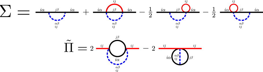
Figure 2: Diagrammatic representation of the fermion ($\Sigma$) and regularized gauge field ($\tilde{\Pi}=\Pi(i\Omega_{m})-\Pi(i\Omega_{m}=0)$) self-energies for the Dyson equation (10). The black lines are fermion propagators, the red lines are gauge field propagators, and the dashed blue lines are contractions of the gaussian random variables $t^{\alpha\beta}_{ij}$ coming from the disorder average. These are the only diagrams that contribute in in the large-$M,N$ limit.

Note that the zero Matsubara frequency component of $A_{ij}$ does not contribute to the action (7) or (9) even at $T\neq 0$. The gauge field contribution to the fermion self energy $\Sigma(i\omega_{n})$ in (10) thus doesn’t involve the zero Matsubara frequency component of the gauge field propagator. This is because, as far as the fermions are concerned, the zero Matsubara frequency components are just static phase shifts of the $t_{ij}^{\alpha\beta}$, and have already been accounted for while disorder averaging. This absence of the zero frequency components has consequences for the thermodynamic properties of the saddle-point solution, and certain modifications have to be made to ensure that the saddle-point is thermodynamically stable (see Sec. IV). However, these modifications do not affect the saddle-point solution to be detailed in the next section above some energy scale which can be made arbitrarily small.

If we consider fluctuations $(\delta G_{i}(i\omega_{n}),\delta\Sigma_{i}(i\omega_{n}))$ about the saddle-point action that do not amount to simply changing a gauge, the kernel of their action at quadratic order is given by $\hat{K}_{ij}=\hat{K}^{(1)}\delta_{ij}+\hat{K}^{(2)}$, where $\hat{K}^{(1,2)}$ are matrices in $(\delta G,\delta\Sigma)$ and frequency space. Here $\hat{K}^{(1)}$ is of order $M$, coming from the fermion determinant and $\Sigma G$ terms of (9), and $\hat{K}^{(2)}$, which comes from the other two terms is of order $1$. Then, diagonalizing $\hat{K}$ in $i,j$ and $(\delta G,\delta\Sigma)$ space produces $\mathcal{O}(N)$ fluctuation eigenmodes with eigenvalues that are $\mathcal{O}(M)$. Integrating over these $N$ modes yields a sub-leading $\mathcal{O}(N)$ contribution to the free energy, and each of these modes also has an $\mathcal{O}(M)$ stiffness that suppresses its fluctuations. Hence, the saddle-point described by (10) is well-defined.

III Single-particle properties

III.1 Zero temperature

We solve for the fermion and gauge field propagators at $T=0$. We set $\mu=0$ (corresponding to half-filling, see Sec. III.2 for $\mu\neq 0$), and start with an ansatz for $G$ in the IR at $T=0$,

$$G(\tau)=-C\frac{\mathrm{sgn}(\tau)}{t^{1-x}|\tau|^{1-x}},~{}~{}G(i\omega_{n})=-2iCt^{x-1}\sin\left(\frac{\pi x}{2}\right)\Gamma(x)\mathrm{sgn}(\omega_{n})|\omega_{n}|^{-x},~{}~{}0<x<\frac{1}{2},~{}~{}C>0.$$ (11)

We then obtain

$$\Pi(i\Omega_{m})-\Pi(i\Omega_{m}=0)=-4(M/N)C^{2}t^{2x}\sin(\pi x)\Gamma(2x-1)\left|\Omega_{m}\right|^{1-2x}.$$ (12)

This the the fermion self-energy

$$\Sigma(i\omega_{n})=\frac{iN\sqrt{\pi}2^{2x-1}\sin\left(\frac{\pi x}{2}\right)\csc^{2}(\pi x)}{2MCx\Gamma(2x-1)\Gamma\left(\frac{1}{2}-x\right)}\mathrm{sgn}(\omega_{n})t^{1-x}\left|\omega_{n}\right|^{x}+t^{2}G(i\omega_{n})\left[1-\int\frac{d\Omega_{m}}{2\pi}\frac{1}{\Pi(i\Omega_{m})-\Pi(i\Omega_{m}=0)}\right].$$ (13)

The integral over $\Omega_{m}$ contains contributions from frequencies outside the regime of validity of the IR solution, and hence requires a UV completion in order to be evaluated. We assume that the UV completion is such that the term in square brackets evaluates to zero, which we will justify below; the vanishing of the square bracketed term is also confirmed by our numerical analysis of the UV complete theory below. Then, using $G(i\omega_{n})=-1/\Sigma(i\omega_{n})$, we find that we cannot determine $C$ (it cancels between the LHS and RHS of the equation), but we can determine the universal exponent $x$ by solving

$$\frac{1/x-2}{1+\sec(\pi x)}=\frac{2M}{N},$$ (14)

with $x$ vs $2M/N$ plotted in Fig. 3. The fact that we can’t determine $C$ purely from the IR properties indicates that it is non-universal.

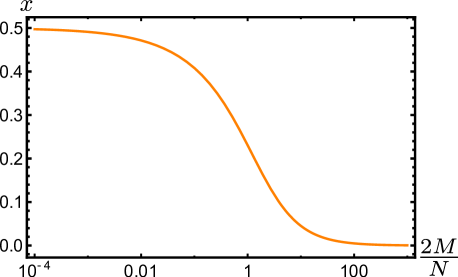
Figure 3: Plot of the exponent $x$ giving the frequency scaling of the IR fermion self-energy, vs $2M/N$, at half-filling.

We now justify the vanishing of the term in square brackets in (13): Suppose it didn’t exactly vanish, and $\int d\Omega_{m}/(\Pi(i\Omega_{m})-\Pi(i\Omega_{m}=0))=1-\nu$, where $\nu\ll 1$. Then, this leaves behind a term $\nu t^{2}G(i\omega_{n})$ in the expression for $\Sigma(i\omega_{n})$, which, scaling as $\mathrm{sgn}(\omega_{n})|\omega_{n}|^{-x}$, is more relevant at low energies than the other term in $\Sigma(i\omega_{n})$. We can then try to ignore the other term in the IR. The Dyson equation becomes

$$\Sigma(i\omega_{n})=\nu t^{2}G(i\omega_{n}),~{}~{}G(i\omega_{n})=\frac{1}{i\omega_{n}-\Sigma(i\omega_{n})},$$ (15)

This equation is solved in the IR by the random-matrix solution $G(i\omega_{n})=-i\mathrm{sgn}(\omega_{n})/(\nu^{1/2}t)$. This solution then modifies the gauge field propagator in the IR, with $\Pi_{\mathrm{new}}(i\Omega_{m})-\Pi_{\mathrm{new}}(i\Omega_{m}=0)=(2/\pi)(M/N)(|\Omega_{m}|/\nu)$. We can then write using (10)

$$\Sigma(i\omega_{n})=-i(t/\nu^{1/2})\mathrm{sgn}(\omega_{n})+i\nu^{1/2}t\int_{-\Lambda}^{\Lambda}\frac{d\Omega_{m}}{2\pi}\frac{\mathrm{sgn}(\omega_{n})-\mathrm{sgn}(\omega_{n}+\Omega_{m})}{(2/\pi)(M/N)|\Omega_{m}|},$$ (16)

where $\Lambda$ is a “critical window” over which the IR solution is valid. This then gives a singular self-energy

$$\Sigma(i\omega_{n})=-i(t/\nu^{1/2})\mathrm{sgn}(\omega_{n})\left(1+\frac{N\nu}{2M}\ln\left(\frac{|\omega_{n}|}{\Lambda}\right)\right)\rightarrow-i(t/\nu^{1/2})\mathrm{sgn}(\omega_{n})\left(\frac{|\omega_{n}|}{\Lambda}\right)^{\frac{N\nu}{2M}},$$ (17)

We have thus recovered a power-law self-energy without explicitly assuming $\nu=0$ to begin with. Repeated iterations of (10) then converge the exponent of the power-law to the value defined by (14).

The Dyson equations (10) are not fully UV-complete, and do not contain enough information to determine the gauge field propagator at high frequencies. In order to solve them numerically, we need a UV-complete set of equations. We do this by adding a “Maxwell” term to the gauge field action

$$S\rightarrow S+\frac{1}{2g^{2}}\int d\tau\sum_{ij=1,i\leq j}^{N}(\partial_{\tau}A_{ij}(\tau)+A^{0}_{i}(\tau)-A^{0}_{j}(\tau))^{2},$$ (18)

with a gauge coupling $g$, and the $A^{0}_{i}$’s may be ignored due to the aforementioned screening. This then adds a term $\Omega_{m}^{2}/g^{2}$ to $\Pi(i\Omega_{m})-\Pi(i\Omega_{m}=0)$ in (10). Note that (18) contains only “electric” kinetic terms for the gauge fields and no “magnetic” terms that are functions of the sums of gauge link variables $A_{ij}$ around closed loops. We will discuss the effects of adding magnetic terms in Sec. IV.

The numerical solution was then performed by starting with free fermion and gauge field Green’s functions

$$G_{0}(i\omega_{n})=\frac{1}{i\omega_{n}+\mu},~{}~{}D_{0}(i\Omega_{m})=\frac{g^{2}}{\Omega_{m}^{2}},$$ (19)

and then iterating the Dyson equations (10) in the MATLAB code gd.m Patel (2018a). We found that the $t^{2}G(i\omega_{n})$ term in $\Sigma(i\omega_{n})$ indeed cancels out as $T\rightarrow 0$, and a power-law scaling of $G(i\omega_{n})$ is obtained in the IR, with the exponent given by (14). This cancellation of the $t^{2}G(i\omega_{n})$ term holds even for $\mu\neq 0$, leading to the results in Sec. III.2. A $T=0$ numerical solution of the real time version of the Dyson equations (performed in gdrealtime0.m Patel (2018b)) also yields the appropriate analytically continued version of (11) for the retarded Green’s function in the IR,

$$G^{R}(\omega)=-2iCt^{x-1}\sin\left(\frac{\pi x}{2}\right)\Gamma(x)(-i\omega)^{-x}.$$ (20)

At the saddle point, we have the effective action for the fluctuations of the $A_{ij}$ fields

$$S_{\mathrm{SP}}^{A}=t^{2}\frac{M}{N}\int d\tau d\tau^{\prime}\sum_{ij=1,i\leq j}^{N}A_{ij}(\tau)\left[G(\tau-\tau^{\prime})G(\tau^{\prime}-\tau)-\delta(\tau-\tau^{\prime})\int d\tau^{\prime\prime}G(\tau-\tau^{\prime\prime})G(\tau^{\prime\prime}-\tau)\right]A_{ij}(\tau^{\prime})$$ (21)

Under the scaling $\tau\rightarrow b\tau$, we have $G(\tau)\rightarrow b^{x-1}G(\tau)$ from (11), which then implies $A_{ij}(\tau)\rightarrow b^{-x}A_{ij}(\tau)$ from (21). Corrections to (21) coming from the expansion of $e^{i(A_{ij}(\tau)-A_{ij}(\tau^{\prime}))}$ beyond quadratic order in (2) are of the form $\int d\tau d\tau^{\prime}c_{n>2}(A_{ij}(\tau)-A_{ij}(\tau^{\prime}))^{n>2}G(\tau-\tau^{\prime})G(\tau^{\prime}-\tau)$. The above scaling then implies that $c_{(n>2)}\rightarrow b^{(n-2)x}c_{(n>2)}$, so these terms are irrelevant, and their coefficients become small in the IR as $b\rightarrow 0$, allowing us to ignore them.

III.2 Deviations from half-filling

For $\mu\neq 0$, the IR Green’s function develops a spectral asymmetry, with $G(-\tau<0)=-e^{-2\pi\mathcal{E}}G(\tau>0)$ at $T=0$;

$$G(\tau>0)=-\frac{C(\mathcal{E})}{t^{1-x}\tau^{1-x}},~{}~{}G(\tau<0)=\frac{C(\mathcal{E})e^{-2\pi\mathcal{E}}}{t^{1-x}|\tau|^{1-x}}.$$ (22)

The polarization $\Pi_{ij}(\tau)$ and the gauge field propagator however remain symmetric about $\tau=0$. The real part of the self energy satisfies $\mathrm{Re}[\Sigma(i\omega_{n}\rightarrow 0)]=\mu$, cancelling the chemical potential in the Green’s function. The $t^{2}G(i\omega_{n})$ term in the self-energy $\Sigma(i\omega_{n})$ still cancels out as before. However, interestingly, the exponent $x$ of the power-law scaling depends on the asymmetry parameter $\mathcal{E}$ and is given by the solution to

$$\frac{(1/x-2)(\cosh(2\pi\mathcal{E})-\cos(\pi x))}{\tan(\pi x)\sin(\pi x)}=\frac{2M}{N}.$$ (23)

This relation can be determined from the Dyson equation (10) following Ref. Sachdev and Ye (1993), and gives $x\rightarrow 1/2$ as $\mathcal{E}\rightarrow\pm\infty$ regardless of $M/N$.

As in the SYK models Sachdev (2015); Davison et al. (2017), the relationship between $\mathcal{E}$ and $\mu$ is nonuniversal, and depends on the values of UV details. However, following Ref. Georges et al. (2001), a universal relationship between the asymmetry parameter and the filling can be determined: The filling $q_{0}$ can be written as

$$q_{0}=i\int_{-\infty}^{\infty}\frac{dE}{2\pi}G^{F}(E)e^{iE0^{+}},$$ (24)

where

$$G^{F}(E)\equiv\int_{-\infty}^{\infty}\frac{dE_{1}}{2\pi}\frac{\rho_{f}(E_{1})}{E_{1}-E-i0^{+}\mathrm{sgn}(E_{1})}$$ (25)

is the Feynman Green’s function, with $\rho_{f}(E_{1})\equiv-2\mathrm{Im}[G^{R}(E_{1})]$ the fermion spectral function. As in Ref. Georges et al. (2001), we have

$$q_{0}=\frac{1}{\pi}(\mathrm{arg}[G^{R}(0^{-})]-\mathrm{arg}[G^{R}(-\infty)])+i\mathcal{P}\int_{-\infty}^{\infty}\frac{dE}{2\pi}\frac{\partial_{E}G^{R}(E)}{G^{R}(E)}e^{iE0^{+}}-i\mathcal{P}\int_{-\infty}^{\infty}\frac{dE}{2\pi}G^{F}(E)\partial_{E}\Sigma^{F}(E)e^{iE0^{+}},$$ (26)

where $\mathcal{P}$ denotes the Cauchy principal value. Obtaining the low-energy forms of $G^{R}(E)$ and hence $\rho_{f}(E)$ from (22), and using $G^{R}(E\rightarrow\pm\infty)=1/(E+i0^{+})$, this can then be written as

$$q_{0}=1+\frac{x}{2}+\mathrm{arg}[-i\sin(\pi(x/2-i\mathcal{E}))e^{-i\pi x/2}]-i\mathcal{P}\int_{-\infty}^{\infty}\frac{dE}{2\pi}G^{F}(E)\partial_{E}\Sigma^{F}(E)e^{iE0^{+}}.$$ (27)

The remaining integral needs to be computed carefully using the Dyson equation (10) and the methods described in Appendix A of Ref. Georges et al. (2001). We obtain

$$q_{0}=1+\frac{x}{2}+\mathrm{arg}[-i\sin(\pi(x/2-i\mathcal{E}))e^{-i\pi x/2}]-\frac{2N\kappa(x)\Gamma^{2}(x)\sin(2\pi x)\sinh(2\pi\mathcal{E})}{M\Gamma(2x-1)},$$ (28)

where $\kappa(x)=\sum_{i=1}^{6}\mathcal{I}_{i}(x)$, with

$$\mathcal{I}_{1}=-\frac{\cot(\pi x)\Gamma(1-x)\Gamma(2x)}{16\pi^{2}\Gamma(1+x)},~{}~{}\mathcal{I}_{2}=-\frac{\csc(\pi x)\Gamma(2x)(\gamma_{E}+\psi(1+x))}{16\pi^{2}\Gamma(x)\Gamma(1+x)},$$

$$\mathcal{I}_{3}=-\frac{e^{i\pi x}}{16\pi^{3}}\int_{-\infty}^{-1}dY_{1}\int_{-\infty}^{0}dY_{2}\frac{Y_{1}^{-x}(-Y_{2})^{2x-1}}{(Y_{1}+Y_{2})(1+Y_{1}+Y_{2})},$$

$$\mathcal{I}_{4}=\frac{1}{16\pi^{3}}\int_{-1}^{0}dY_{1}(-Y_{1})^{-x}(Y_{1}+1)^{2x-1}\left(-\frac{\,{}_{2}F_{1}\left(1,1-2x;2-2x;\frac{Y_{1}}{Y_{1}+1}\right)}{2x-1}-\ln(Y_{1}+1)+\gamma_{E}+\psi(1-2x)\right),$$

$$\mathcal{I}_{5}=-\frac{e^{i\pi x}x\Gamma(1-x)}{16\pi^{3}\Gamma(2-x)}\int_{-\infty}^{0}dY_{1}\int_{-\infty}^{0}dY_{2}\frac{\theta(-Y_{1}-Y_{2}-1)}{(Y_{1}+Y_{2})^{2}}Y_{1}^{-x}(-Y_{2})^{2x-1}\,_{2}F_{1}\left(1,1-x;2-x;-\frac{1}{Y_{1}+Y_{2}}\right),$$

$$\mathcal{I}_{6}=-\frac{e^{i\pi x}x}{16\pi^{3}(1+x)}\int_{-\infty}^{0}dY_{1}\int_{-\infty}^{0}dY_{2}~{}\theta(Y_{1}+Y_{2}+1)Y_{1}^{-x}(-Y_{2})^{2x-1}\,_{2}F_{1}\left(1,1+x;2+x;-(Y_{1}+Y_{2})\right),$$ (29)

where $\psi$ is the digamma function, $\theta$ is the Heaviside step function, $\,{}_{2}F_{1}$ is a hypergeometric function hyp , and $\gamma_{E}$ is the Euler-Mascheroni constant. $\kappa(x\rightarrow 1/2)=-1/(16\pi)$, and $\kappa(x\rightarrow 0)\propto-1/x^{2}$ (see Fig. 4b). Putting together (23), (28) and (29), we see that $q_{0}$ is a smooth function of $\mathcal{E}$ that decreases monotonically from $1$ to $0$ as $\mathcal{E}$ is swept from $-\infty$ to $\infty$ (see Fig. 4a). This dependence of $q_{0}$ on $\mathcal{E}$ also agrees quantitatively with that obtained from the numerical solutions of (10), in which $q_{0}$ is given by $q_{0}=G(\tau=0^{-})$ and $e^{-2\pi\mathcal{E}}=\mathrm{Im}[G^{R}(\omega=0^{-})]/\mathrm{Im}[G^{R}(\omega=0^{+})]$.

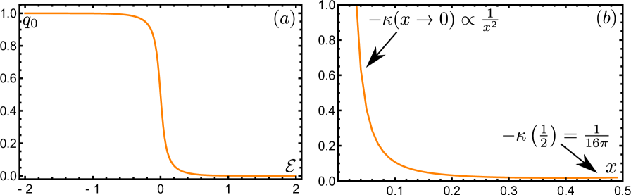
Figure 4: (a) Plot of the filling $q_{0}$ vs the asymmetry parameter $\mathcal{E}$ for $2M=N$. (b) Plot of the function $-\kappa(x)$ defined in (29) vs the self-energy exponent $x$.

III.3 Nonzero temperature

The regularized IR Dyson equations (10) can be written in the time domain using two-time notation as (see Ref. Sachdev (2015))

$$-\int d\tau_{3}G(\tau_{1},\tau_{3})\tilde{\Sigma}(\tau_{3},\tau_{2})=\delta(\tau_{1},\tau_{2}),~{}~{}\tilde{\Sigma}(\tau_{1},\tau_{2})=t^{2}\nu G(\tau_{1},\tau_{2})+t^{2}G(\tau_{1},\tau_{2})D(\tau_{2},\tau_{1})$$

$$\int d\tau_{3}D(\tau_{1},\tau_{3})\tilde{\Pi}(\tau_{3},\tau_{2})=\tilde{\delta}(\tau_{1},\tau_{2}),~{}~{}\tilde{\Pi}(\tau_{1},\tau_{2})=2t^{2}\frac{M}{N}\left(G(\tau_{1},\tau_{2})G(\tau_{2},\tau_{1})-\delta(\tau_{1},\tau_{2})\int d\tau_{3}G(\tau_{1},\tau_{3})G(\tau_{3},\tau_{2})\right),$$ (30)

where

$$\nu=1-\lim_{2\rightarrow 1}[D(\tau_{1},\tau_{2})+D_{\mathrm{UV}}(\tau_{1},\tau_{2})],$$ (31)

and $\tilde{\delta}(\tau_{1},\tau_{2})=\delta(\tau_{1},\tau_{2})-L^{-1}_{\tau}$, where $L_{\tau}$ is the length of the time domain ($L^{-1}_{\tau}=T$ at a finite temperature $T$). The chemical potential $\mu$ has been absorbed into $\Sigma$ to regularize it to $\tilde{\Sigma}$. We split the gauge field propagator into an IR piece $D$ and a UV piece $D_{\mathrm{UV}}$. The UV piece is not determined by (30), and is not sensitive to rescalings of $\tau$. The reason that the $\tilde{\delta}$ appears instead of just a $\delta$ is because the action (7) doesn’t contain zero frequency modes of $A_{ij}$. As a result, $D$ here doesn’t contain a zero frequency mode either, and consequently the pertinent delta function should be modified to remove its zero frequency mode. On a time domain of infinite size (such as at zero temperature), the zero frequency mode occupies a measure zero subspace, and then there is no difference between $\tilde{\delta}$ and $\delta$.

The equations (30) are not invariant under a general set of reparametrizations with $\tau=f(\sigma)$ and an arbitrary function $h$, Sachdev (2015)

$$G(\tau_{1},\tau_{2})\rightarrow\frac{h(\sigma_{1})/h(\sigma_{2})}{(f^{\prime}(\sigma_{1})f^{\prime}(\sigma_{2}))^{a}}G(\sigma_{1},\sigma_{2}),~{}~{}\tilde{\Sigma}(\tau_{1},\tau_{2})\rightarrow\frac{h(\sigma_{1})/h(\sigma_{2})}{(f^{\prime}(\sigma_{1})f^{\prime}(\sigma_{2}))^{1-a}}\tilde{\Sigma}(\sigma_{1},\sigma_{2}),$$

$$D(\tau_{1},\tau_{2})\rightarrow(f^{\prime}(\sigma_{1})f^{\prime}(\sigma_{2}))^{2a-1}D(\sigma_{1},\sigma_{2}),~{}~{}\tilde{\Pi}(\tau_{1},\tau_{2})\rightarrow(f^{\prime}(\sigma_{1})f^{\prime}(\sigma_{2}))^{-2a}\tilde{\Pi}(\sigma_{1},\sigma_{2}),$$ (32)

because of the second term in the expression for $\tilde{\Pi}$, and additionally because $\nu$ and $L^{-1}_{\tau}$ can be nonzero. However, they can still be scale invariant under $\tau\rightarrow b\tau$ iff

$$G\rightarrow b^{-2a}G,~{}~{}\tilde{\Sigma}\rightarrow b^{2a-2}\tilde{\Sigma},~{}~{}D\rightarrow b^{4a-2}D,~{}~{}\tilde{\Pi}\rightarrow b^{-4a}\tilde{\Pi},~{}~{}\nu\rightarrow b^{4a-2}\nu.$$ (33)

Note that $a$ is not determined by these equations, but we choose $2a=1-x$ due to the particular power-law scaling of Sec. III.1 that is selected when the UV-complete equations are solved.

Now consider applying the scale transformation at a finite temperature. Since $\tau\in[0,1/T)$, this also scales $T\rightarrow T/b$, leaving $T\tau$ invariant. (30) is then compatible with a scaling solution (reverting back to one-time notation) $G(\tau)\propto T^{1-x}F_{G}(\tau T)$ (and corresponding expressions for $D$, $\tilde{\Sigma}$ and $\tilde{\Pi}$) iff $\nu\propto T^{2x}$. To check that we indeed get this behavior of $\nu$, we use the definition (31) of $\nu$, the fact that $D_{\mathrm{UV}}$ is not affected by rescalings of $T$ at low $T\ll\Lambda$, and the scaling form for $D(\tau)\propto T^{2x}F_{D}(\tau T)$, to obtain

$$\nu(T)-\nu(0)=\lim_{T\rightarrow 0}\lim_{\tau\rightarrow 0}[T^{2x}F_{D}(\tau T)]-\lim_{\tau\rightarrow 0}T^{2x}F_{D}(\tau T),$$ (34)

which gives $\nu(T)\propto T^{2x}$ when $\nu(0)=0$, which we already established in Sec. III.1. Thus, the low-energy Dyson equations in the gauge field problem are fully consistent with a scaling solution at small finite temperatures. Our numerical solution confirms this (Fig. 5a), and we also find $\nu(T)\sim T^{2x}$ numerically at small $T$ (Fig. 5b).

The IR fermion Green’s function in the gauge field case does not have a conformally remapped form at $T\neq 0$, as the equations (30) are not invariant under (32) with $\tau=\tan(\pi T\sigma)/T$, but instead obeys

$$G(i\omega_{n},T)=\frac{C(\mathcal{E})}{t^{1-x}T^{x}}F_{G}\left(\frac{\omega_{n}}{T},\mathcal{E}\right),~{}~{}F_{G}(y\rightarrow 0,\mathcal{E})\propto y^{0},~{}~{}F_{G}(y\rightarrow\infty,\mathcal{E})\propto\frac{1}{y^{x}}.$$ (35)

We can only compute the scaling function $F_{G}$ numerically. The self-energy also satisfies a low-energy scaling form $\mathrm{Im}[\Sigma(i\omega_{n})]=-C^{-1}(\mathcal{E})t^{1-x}T^{x}F_{\Sigma}(\omega_{n}/T,\mathcal{E})$. However, the scaling function $F_{\Sigma}$ again differs from the conformal scaling function for the same exponent $x$ (corresponding to the self-energy $\Sigma_{c}(i\omega_{n})=-1/G_{c}(i\omega_{n})$ derived from the conformal Green’s function $G_{c}(\tau)=-(C\pi^{1-x}/t^{1-x})(T/\sin(\pi T|\tau|))^{1-x}$), as can be seen by comparing universal ratios such as $n_{31}\equiv\mathrm{Im}[\Sigma(3i\pi T)]/\mathrm{Im}[\Sigma(i\pi T)]$ with their corresponding conformal values (see Table 1).

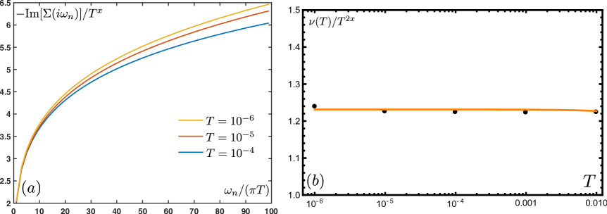
Figure 5: (a) Plot of the scaling form of the fermion self-energy $C^{-1}(0)t^{1-x}F_{\Sigma}(\omega_{n}/T,0)\equiv-\mathrm{Im}[\Sigma(i\omega_{n})]/T^{x}$ vs $\omega_{n}/(\pi T)$ obtained by numerical solution of the imaginary-time Dyson equations for different values of $T$. For all curves, $t=g^{2}=1$, $2M=N$ and $\mu=0$ (corresponding to $x=0.230651$ from (14)). The curves collapse onto one another at low frequencies, confirming a universal low-energy scaling form. The deviations from universality at higher frequencies and temperatures occur because of the finite size of the critical window $\Lambda$ over which the low-energy solution is valid. (b) Plot of the quantity $\nu(T)/T^{2x}$ vs $T$ for the same values of parameters. This clearly shows $\nu(T)\propto T^{2x}$ over a large range of temperatures.

Ratio	$T=10^{-4}$	$T=10^{-5}$	$T=10^{-6}$	Conformal
$n_{31}$	1.3680	1.3703	1.3709	1.2607
$n_{53}$	1.1363	1.1382	1.1387	1.1224
$n_{75}$	1.0845	1.0862	1.0865	1.0800
$n_{97}$	1.0611	1.0626	1.0629	1.0594

Table 1: Comparision of numerical values of ratios $n_{ab}\equiv\mathrm{Im}[\Sigma(ia\pi T)]/\mathrm{Im}[\Sigma(ib\pi T)]$ in the gauge field problem at different temperatures with those derived from the conformal Green’s function $G_{c}(\tau)=-(C\pi^{1-x}/t^{1-x})(T/\sin(\pi T|\tau|))^{1-x}$). As $T$ is reduced, these ratios converge to universal values that differ significantly from the conformal ones at low energies, which implies that the scaling function $F_{\Sigma}$ (or $F_{G}$) is not the conformal one, and that the local criticality in the gauge field model is different from the SYK universality class. The values of other parameters used are the same as those used in Fig. 5, but these universal low-energy ratios are insensitive to the values of $t$ and $g^{2}$ as $T\rightarrow 0$ within numerical tolerances.

IV Thermodynamics

In this section we describe the thermodynamic properties of the saddle-point solution described in the previous two sections at low temperatures. We specialize to the case of half-filling, with $\mu=0$. This allows for temperature derivatives of the free energy at a constant fermion density of half-filling to be the same as its temperature derivatives at constant zero chemical potential, which are easier to evaluate. We do not expect any of the qualitative features discussed here to be modified away from half-filling.

The free energy can be written down from (9) evaluated at the saddle-point. It is

$$\mathcal{F}=-T\ln Z=MNT\sum_{\omega_{n}}\ln\left[\frac{i\omega_{n}}{i\omega_{n}-\Sigma_{i}(i\omega_{n})}\right]-MNT\ln 2+t^{2}\frac{MN}{2}T\sum_{\omega_{n}}G^{2}(i\omega_{n})-MNT\sum_{\omega_{n}}\Sigma(i\omega_{n})G(i\omega_{n})$$

$$+\frac{N^{2}T}{4}\sum_{\Omega_{m}\neq 0}\ln\left[\Pi(i\Omega_{m})-\Pi(i\Omega_{m}=0)\right],$$ (36)

where we added and subtracted the free fermion contribution, so that the frequency sum involving the logarithm converges and we may evaluate it numerically. The term on the second lime represents the gauge field contribution. Setting this aside for the moment, and numerically evaluating the fermion contribution using the saddle point of the UV complete action with the electric “Maxwell” term (18), we obtain $\mathcal{F}_{f}/(MN)\approx-c_{0}(M/N)+Tc_{1}(M/N)$ as $T\rightarrow 0$. This implies that the fermion contribution to the specific heat $\mathcal{C}_{f}=-T\partial^{2}\mathcal{F}_{f}/\partial T^{2}$ vanishes at low temperatures and the fermions make a constant negative contribution $\mathcal{S}_{f}=-\partial\mathcal{F}_{f}/\partial T$ to the total entropy. Since the fermions and gauge fields are highly entangled, we of course need to add the gauge field contribution to obtain the full physical free energy and associated thermodynamic quantities. We can write

$$\mathcal{F}_{A}=\frac{N^{2}T}{4}\sum_{\Omega_{m}\neq 0}\ln\left[\frac{\Pi(i\Omega_{m})-\Pi(i\Omega_{m}=0)}{\Pi(i\Omega_{m},T=0)-\Pi(i\Omega_{m}=0,T=0)}\right]+\frac{N^{2}T}{4}\sum_{\Omega_{m}\neq 0}\ln\left[\Pi(i\Omega_{m},T=0)-\Pi(i\Omega_{m}=0,T=0)\right],$$ (37)

where we have added and subtracted a term that is evaluated using the zero temperature functional form of $\Pi$, but evaluated at the Matsubara frequencies corresponding to a particular temperature. Since $\Pi(i\Omega_{m})-\Pi(i\Omega_{m}=0)$ obeys a quantum-critical scaling form, the first term becomes $\mathcal{F}_{A}^{(1)}/(MN)=-\frac{NT}{4M}\sum_{m\neq 0}\ln[(2\pi m)^{1-2x}F_{D}(2\pi m)]$. We find numerically that $F_{D}(2\pi m)=1/(2\pi m)^{1-2x}+\mathcal{O}(1/m^{2})$ for $m\gg 1$ in the scaling limit, so this sum converges at large $m$, and leads to $\mathcal{F}^{(1)}_{A}/(MN)\sim-T$, which doesn’t contribute to the specific heat and provides a constant contribution to the entropy at low temperatures.

The second term of (37) can be computed by zeta-function regularization using the result (12):

$$\frac{\mathcal{F}_{A}^{(2)}}{MN}=\frac{NT}{4M}\sum_{m\neq 0}\ln\left[-4\frac{M}{N}C^{2}t^{2x}\sin(\pi x)\Gamma(2x-1)\left|2\pi m\right|^{1-2x}T^{1-2x}\right]$$

$$=-\frac{NT}{4M}\ln\left[-4\frac{M}{N}C^{2}t^{2x}\sin(\pi x)\Gamma(2x-1)T^{1-2x}\right].$$ (38)

This produces the dominant contribution to the low-temperature specific heat,

$$\frac{\mathcal{C}}{MN}\approx\frac{\mathcal{C}_{A}^{(2)}}{MN}=-T\frac{\partial^{2}\mathcal{F}_{A}^{(2)}}{\partial T^{2}}=\frac{(1-2x)N}{4M},$$ (39)

which is positive and extensive. In the limit of $M/N\rightarrow\infty$, where $x\rightarrow 0$ and the non-Fermi liquid solution turns into a noninteracting random matrix solution, this large contribution to the specific heat vanishes as it should, and in the opposite limit of $M/N\rightarrow 0$, where $x\rightarrow 1/2$, it blows up as $1/\sqrt{M/N}$, as can be seen by applying (14).

The free energy contribution $\mathcal{F}_{A}^{(2)}$ also leads to the dominant contribution to the low-temperature entropy $\mathcal{S}_{A}^{(2)}/(MN)=-\partial\mathcal{F}_{A}^{(2)}/\partial T\propto(1-2x)(N/(4M))\ln T$. This is negative at low $T$, which indicates that our theory is incomplete: extra degrees of freedom must be present in a physical theory in order to offset this entropy. The reason this happens is that our theory is missing all information about the zero-frequency modes of the $A_{ij}$. In any sensible electromagnetic lattice gauge theory, these modes will contribute to physical static magnetic field configurations that cost energy: Exciting a single link $A_{ij}$ will lead to nonzero magnetic fluxes through all plaquettes containing that link, and a magnetic “Maxwell” term acting on these fluxes will contribute to the action, even if they are static. However such terms are not generated in our theory by integrating out the fermions in the large-$N$,$M$ limits. In order to generate these terms we need to appeal to some heavy degrees of freedom that couple to the gauge fields in such a way that integrating out these degrees of freedom will produce magnetic “Maxwell” terms.

Assuming this is the case, we write down the simplest possible gauge and time-reversal invariant magnetic “Maxwell” action that is appropriate for an all-to-all interacting theory without any spatial structure. It is

$$S_{B}=\frac{m^{2}_{B}}{2(N-2)}\int d\tau\sum_{\triangle ijk}(A_{ij}(\tau)+A_{jk}(\tau)+A_{ki}(\tau))^{2},$$ (40)

where the sum runs over all possible unique triangles. The kernel of this quadratic action has $(N-1)(N-2)/2$ degenerate eigenvectors with eigenvalue $m_{B}^{2}(1+2/(N-2))$ and $N-1$ degenerate eigenvectors with eigenvalue $0$. The zero-eigenvalued eigenvectors are all pure gauge and can each be gauge-transformed to the configuration $A_{ij}=0$; they correspond to the state in which the flux through all triangles is zero, and thus do not contribute anything to the free energy. In the large-$N$ limit, the thermodynamic fraction of modes residing on a single links $A_{ij}$ have negligible overlap with the zero-eigenvalued eigenvectors. This permits the approximation, exact in the infinite-$N$ limit

$$S_{B}\approx\frac{m^{2}_{B}}{2}\int d\tau\sum_{ij=1,i\leq j}^{N}A_{ij}^{2}(\tau).$$ (41)

We assume that $m^{2}_{B}$ is much smaller than $-4(M/N)C^{2}\sin(\pi x)\Gamma(2x-1)t^{2x}T^{1-2x}$. Then including this term just adds

$$\mathcal{F}_{A}^{(3)}=\frac{N^{2}}{4}T\ln m^{2}_{B}$$ (42)

to (36). This term doesn’t contribute to the specific heat, but offsets the leading contribution to the entropy to a large positive value $\mathcal{S}_{A}^{(2)+(3)}/(MN)=(N/(4M))\ln(-4(M/N)C^{2}\sin(\pi x)\Gamma(2x-1)t^{2x}T^{1-2x}/m^{2}_{B})$.

For $-4(M/N)C^{2}\sin(\pi x)\Gamma(2x-1)t^{2x}T^{1-2x}\ll m_{B}^{2}$, the fermions effectively end up coupling to gapped bosonic modes. The low-energy Dyson equation then reads

$$\Sigma(i\omega_{n})=t^{2}G(i\omega_{n})\left[1-T\sum_{\Omega_{m}\neq 0}\frac{1}{m_{B}^{2}+\Pi(i\Omega_{m})-\Pi(i\Omega_{m}=0)}\right]+t^{2}T\sum_{\Omega_{m}\neq 0}\frac{G(i\omega_{n}+i\Omega_{m})}{m_{B}^{2}+\Pi(i\Omega_{m})-\Pi(i\Omega_{m}=0)},$$

$$\Pi(i\Omega_{m})=2t^{2}T\frac{M}{N}\sum_{\omega_{n}}G(i\omega_{n})G(i\omega_{n}+i\Omega_{m}),~{}~{}G(i\omega_{n})=\frac{1}{i\omega_{n}+\mu-\Sigma(i\omega_{n})}.$$ (43)

The term in square brackets no longer cancels at $T=0$, as increasing the denominator of the boson propagator by adding a mass makes its value smaller than the zero-mass case. This leaves behind a $\nu t^{2}G(i\omega_{n})$ term in $\Sigma(i\omega_{n})$, leading to a renormalized random-matrix solution at the lowest energies. The second term in the first line of (43) vanishes at small external frequencies $\omega_{n}$, as $G(i\Omega_{m})$ is odd in $\Omega_{m}$ and the denominator is a constant at low frequencies (for nonzero chemical potential, this sum just produces a constant that is absorbed by $\mu$). These points can be easily verified by numerically solving the UV-completed version of (43) using the MATLAB code gd.m Patel (2018a). The lowest energy state then has a vanishing entropy and specific heat. Henceforth, we shall assume that we are only interested in energy scales larger than the small $m^{2}_{B}$, treating it as an IR regulator much smaller than $T$, and focus on the non-Fermi liquid.

We also checked numerically that the compressibility $MN\partial q_{0}/\partial\mu|_{T}$, where $q_{0}=G(\tau=0^{-})$ asymptotes to a nonzero constant as $T\rightarrow 0$. This justifies our rationale of ignoring the time components $A^{0}_{i}$ of the gauge fields in the IR, as their propagators are screened by this compressibility.

Finally, from the point of view of the magnetic “Maxwell” terms, the model behaves like a U(1) gauge theory in a large ($\mathcal{O}(N)$) number of dimensions. Possible magnetic monopoles arising due to the compactness of the U(1) gauge group then source nonzero fluxes through a large number of plaquettes, leading to $\mathcal{O}(N)$ increases in the free energy through the magnetic Maxwell terms, while not coupling to the fermions by virtue of being a static background. Thus, the configuration in which no monopoles exist should be a stable saddle-point, and monopole operators are irrelevant.

V Transport

In order to consider transport properties of this model, we need to make appropriate modifications. First, we need some spatial structure. This can be achieved by defining the clusters indexed by $i,j$ to lie on the sites of an $N$-dimensional hypercubic lattice, with each cluster then having $2N$ neighbors. The fermions hop between nearest neighbor clusters, coupling to gauge fields $A_{ij}$ that live on the bonds of the lattice. Second, for an external probe gauge field to drive a current, it must couple to a different charge from the one that the internal gauge fields $A_{ij}$ couple to: If they coupled to the same charge, then turning on the probe field only amounts to shifting the values of $A_{ij}$, and the path integral over $A_{ij}$ trivially absorbs these shifts, rendering the partition function immune to the probe field. If we view the fermions as chargons arising from fractionalization in an ACL, we can divide the flavors indexed by $\alpha,\beta$ into equal fractions of two species that couple to the internal gauge field with opposite charges, but which couple to the external probe gauge field with equal charges, which is a single-axis version of the SU(2) case discussed in Ref. Sachdev (2018). Then, our modified version of (1) reads

$$\mathcal{H}^{\prime}=-\frac{1}{(2MN)^{1/2}}\sum_{\langle ij\rangle}\sum_{\alpha\beta=1}^{M}\sum_{ss^{\prime}=\pm}\left[t_{ij}^{\alpha\beta}f^{\dagger}_{i\alpha s}e^{iA_{ij}\sigma^{z}_{ss^{\prime}}}f_{j\beta s^{\prime}}+(2MN)^{1/2}\mu\delta_{ij}^{\alpha\beta}\delta_{ss^{\prime}}f^{\dagger}_{i\alpha s}f_{i\alpha s}\right],$$

$$\ll t_{ij}^{\alpha\beta}t_{ji}^{\beta\alpha}\gg=\ll|t_{ij}^{\alpha\beta}|^{2}\gg=t^{2}.$$ (44)

This has a U(1) gauge invariance under $f_{i\alpha s}(\tau)\rightarrow\sum_{s^{\prime}=\pm}e^{i\theta_{i}(\tau)\sigma^{z}_{ss^{\prime}}}f_{i\alpha s^{\prime}}(\tau)$ and $A_{ij}(\tau)\rightarrow A_{ij}(\tau)+\theta_{i}(\tau)-\theta_{j}(\tau)$.

Performing the same manipulations as before, we obtain

$$S^{\prime}=\int d\tau\sum_{i}\sum_{\alpha=1}^{M}\sum_{s=\pm}f^{\dagger}_{i\alpha s}(\tau)(\partial_{\tau}+isA^{0}_{i}(\tau)+\mu)f_{i\alpha s}(\tau)$$

$$+t^{2}\frac{M}{2N}\int d\tau d\tau^{\prime}\sum_{\langle ij\rangle}\sum_{ss^{\prime}=\pm}\left[\left(1-\frac{1}{2}A_{ij}^{2}(\tau)-\frac{1}{2}A_{ij}^{2}(\tau^{\prime})+A_{ij}(\tau)A_{ij}(\tau^{\prime})\right)\delta_{ss^{\prime}}+i(A_{ij}(\tau)-A_{ij}(\tau^{\prime}))\sigma^{z}_{ss^{\prime}}\right]$$

$$\times G_{js^{\prime}}(\tau-\tau^{\prime})G_{is}(\tau^{\prime}-\tau)-M\int d\tau d\tau^{\prime}\sum_{i}\sum_{s=\pm}\Sigma_{is}(\tau-\tau^{\prime})\left[G_{is}(\tau^{\prime}-\tau)-\frac{1}{M}\sum_{\alpha=1}^{M}f_{i\alpha s}(\tau^{\prime})f^{\dagger}_{i\alpha s}(\tau)\right],$$ (45)

as before, the time integrations kill the term proportional to $\sigma^{z}$ in the second line of the above. This action then leads to a saddle-point symmetric in $s$ described by (10), with the IR solution (11). Similar arguments for invariance under gauge-fixing at large-$N$ and stability of the saddle-point as before apply.

We now perturb the action (45) with a diagonal probe field, so that $A_{ij}(\tau)\sigma^{z}_{ss^{\prime}}\rightarrow A_{ij}(\tau)\sigma^{z}_{ss^{\prime}}+\Xi_{ij}(\tau)\delta_{ss^{\prime}}$ where $\Xi_{ij}(\tau)=\delta_{j,i+\hat{x}}\Xi(\tau)$, which corresponds to applying an electric field $\mathbf{E}=-(d\Xi(\tau)/d\tau)\hat{x}$ in the $\hat{x}$ direction. The perturbed action reads

$$S^{\prime}_{\Xi}=-M\sum_{i}\sum_{s=\pm}\mathrm{Tr}\ln[\partial_{\tau}+\mu\delta(\tau,\tau^{\prime})-\Sigma_{is}(\tau,\tau^{\prime})]$$

$$+t^{2}\frac{M}{2N}\int d\tau d\tau^{\prime}\sum_{\langle ij\rangle}\sum_{ss^{\prime}=\pm}\left[\left(1-\frac{1}{2}(A_{ij}(\tau)-A_{ij}(\tau^{\prime}))^{2}\right)\delta_{ss^{\prime}}+i(A_{ij}(\tau)-A_{ij}(\tau^{\prime}))\sigma^{z}_{ss^{\prime}}\right]G_{js^{\prime}}(\tau,\tau^{\prime})G_{is}(\tau^{\prime},\tau)$$

$$+t^{2}\frac{M}{2N}\int d\tau d\tau^{\prime}\sum_{\langle ij\rangle}\sum_{s=\pm}\left[i(\Xi_{ij}(\tau)-\Xi_{ij}(\tau^{\prime}))-\frac{1}{2}(\Xi_{ij}(\tau)-\Xi_{ij}(\tau^{\prime}))^{2}\right]G_{js}(\tau,\tau^{\prime})G_{is}(\tau^{\prime},\tau)$$

$$-t^{2}\frac{M}{2N}\int d\tau d\tau^{\prime}\sum_{\langle ij\rangle}\sum_{ss^{\prime}=\pm}(A_{ij}(\tau)-A_{ij}(\tau^{\prime}))(\Xi_{ij}(\tau)-\Xi_{ij}(\tau^{\prime}))\sigma^{z}_{ss^{\prime}}G_{js^{\prime}}(\tau,\tau^{\prime})G_{is}(\tau^{\prime},\tau),$$ (46)

where we integrated out the fermions and neglected the $A^{0}_{i}$ as before. With the perturbed partition function $Z^{\prime}_{\Xi}=\int\mathcal{D}A\mathcal{D}G\mathcal{D}\Sigma~{}e^{-S^{\prime}_{\Xi}[A,G,\Sigma]}$, we then obtain the current-current correlator

$$\langle J_{x}(\tau)J_{x}(\tau^{\prime})\rangle=\frac{1}{Z^{\prime}_{\Xi=0}}\frac{\delta^{2}Z^{\prime}_{\Xi}}{\delta\Xi(\tau)\delta\Xi(\tau^{\prime})}\Bigg{|}_{\Xi=0}=\int\mathcal{D}A\mathcal{D}G\mathcal{D}\Sigma~{}\frac{e^{-S^{\prime}_{\Xi=0}[A,G,\Sigma]}}{Z^{\prime}_{\Xi=0}}\left(\frac{\delta S^{\prime}_{\Xi}[A,G,\Sigma]}{\delta\Xi(\tau)}\frac{\delta S^{\prime}_{\Xi}[A,G,\Sigma]}{\delta\Xi(\tau^{\prime})}-\frac{\delta^{2}S^{\prime}_{\Xi}[A,G,\Sigma]}{\delta\Xi(\tau)\delta\Xi(\tau^{\prime})}\right)\Bigg{|}_{\Xi=0}.$$ (47)

The only term that survives after integrating out the fields (which makes $G$ and $\Sigma$ take their saddle-point values) is

$$\langle J_{x}(\tau)J_{x}(\tau^{\prime})\rangle=-Vt^{2}\frac{M}{N}\left[G(\tau-\tau^{\prime})G(\tau^{\prime}-\tau)-\delta(\tau-\tau^{\prime})\int d\tau^{\prime\prime}G(\tau-\tau^{\prime\prime})G(\tau^{\prime\prime}-\tau)\right],$$ (48)

where $V$ is the system volume (number of sites in the hypercubic lattice). The right-hand-side of (48) automatically contains the sum of the paramagnetic and diamagnetic terms.

This gives rise to the DC conductivity, employing the scaling forms derived in Sec. III.3,

$$\sigma_{xx}^{\mathrm{DC}}=-\frac{1}{V}\lim_{\mathrm{\Omega_{m}\rightarrow 0}}\frac{\langle J_{x}J_{x}\rangle(i\Omega_{m})}{\Omega_{m}}\sim\frac{M}{N}\left(\frac{t}{T}\right)^{2x},$$ (49)

and the optical conductivity

$$\sigma_{xx}(\Omega\gg T)=-2(M/N)C^{2}\sin(\pi x)\Gamma(2x-1)\left(\frac{it}{\Omega}\right)^{2x}.$$ (50)

As discussed in Sec. II, since the saddle-point value of $G$ is gauge-independent at leading order in large-$N$, this answer for the conductivity is correctly gauge-invariant at leading order in large-$N$. Since the critical solution (35) is in general valid only for $T\ll t$, the DC conductivity (49) is never parametrically in a bad-metallic regime of $\sigma^{\mathrm{DC}}\ll 1$ within the energy window of validity of the non-Fermi liquid solution.

VI Discussion

We have constructed a model of a disordered non-Fermi liquid phase of fermions at a finite density coupled to gapless fluctuating U(1) gauge fields, in a solvable large-$N$ limit. In this non-Fermi liquid phase, both the fermion and photon Green’s functions are gapless, and decay as power-laws of time at long times. The power-law exponents are continuously tunable within a finite range, and, interestingly, depend upon the filling fraction of the fermions.

A special feature of our model is that the non-Fermi liquid phase arises under the combined effect of hopping and interaction terms, in contrast to the purely interacting SYK models. In the SYK models, the addition of quadratic hopping terms results in a weakly-interacting Fermi liquid solution in the infrared Song et al. (2017). However, unlike the SYK models, in which the interaction between the fermions is instantaneous in the large-$N$ limit, the interaction between fermions in our model is retarded, mediated by gapless bosonic modes with singular propagators at low energies, leading to non-Fermi liquid behavior even in the presence of hopping terms Lee (2018).

Our model only possesses scale invariance in the infrared, and not the much more comprehensive time reparametrization invariance of the SYK models. At nonzero temperatures, this lack of time reparametrization symmetry in our model results in different finite temperature fermion Green’s functions from the conformal ones that appear in the generalized set of SYK_q models with $1<q/2<2$-body interactions Maldacena and Stanford (2016); Davison et al. (2017). Consequently, we do not expect our model to have as direct a holographic connection to AdS₂ gravity as the SYK models, or to display maximal chaos Sachdev (2010); Kitaev (2015); Sachdev (2015); Maldacena and Stanford (2016); Kitaev and Suh (2018). However, due to the quantum-critical scaling of the Green’s functions, we still expect the Lyapunov exponent for many-body quantum chaos to be an $\mathcal{O}(1)$ number times $k_{B}T/\hbar$, similar to other models of fermions strongly coupled to fluctuating gauge fields Patel and Sachdev (2017).

The dynamic photon modes cause our model to have a much larger Hilbert space than the SYK models, which only have fermions. This appears to allow for a finer spacing of the low-lying many-body energy levels than in the SYK models (which have a level spacing of $\sim e^{-N}$ Fu and Sachdev (2016)), leading to parametrically larger values of entropy and specific heat at low temperatures, that are dominated by contributions from the photon modes.

We can view our model as a toy model of an ACL Sachdev (2018); Kaul et al. (2008), which is a candidate for the strange metal regime of the cuprate superconductors. This is an effective theory in which electrons are fractionalized into gapless fermionic chargons which carry their charge (but not spin), and gapped bosonic spinons that do not affect the low-energy fluctuations of the chargons. By defining our model on an $N$-dimensional hypercubic lattice, we obtain non-Fermi liquid charge transport properties, with a sub-linear power-law-in-temperature resistivity. The exponent of the power-law is continuously tunable as a function of the filling, and can approach linear-in-temperature for certain parameter ranges. This non-Fermi liquid has a ‘large Fermi surface’, i.e. all $M$ flavors of fermions are active and contribute to transport. This is in contrast to the SYK/Kondo-lattice models of non-Fermi liquids proposed in Refs. Patel et al. (2018a); Chowdhury et al. (2018), where only the itinerant fermions contribute to transport.

For future work, it would be interesting to see if some of the strategies employed here can be extended to construct solvable models of fermions at finite density and with quenched disorder interacting with gauge fields in $2+1$ dimensions. Such models would of course be more realistic candidates for describing the phase diagram of the cuprates. It would also be interesting, if possible, to consider Higgs transitions out of ACLs in such models into weakly interacting ‘pseudogap’ phases with a reduced number of active fermions Sachdev (2018); Chowdhury and Sachdev (2015), along the lines of the analysis in Appendix A.

Appendix A Higgs transition from the U(1) ACL to a $\mathbb{Z}_{2}$ ACL

We consider a Higgs transition that breaks the U(1) gauge invariance down to $\mathbb{Z}_{2}$ in the ACL of Sec. V. This is expected to be a toy model of the optimal doping transition in the cuprates without a symmetry-breaking order parameter, from the overdoped to the underdoped side Sachdev et al. (2009); Chowdhury and Sachdev (2015); Sachdev and Chowdhury (2016); Scheurer et al. (2018). We modify the fermion-gauge field hamiltonian to

$$\mathcal{H}_{1}^{\prime\prime}=-\frac{1}{(2MN)^{1/2}}\sum_{\langle ij\rangle}\sum_{\alpha\beta=1}^{M}\sum_{s=\pm}\left[t_{ijs}^{\alpha\beta}f^{\dagger}_{i\alpha s}e^{isA_{ij}}f_{j\beta s}+(2MN)^{1/2}\mu\delta_{ij}^{\alpha\beta}f^{\dagger}_{i\alpha s}f_{i\alpha s}\right],~{}~{}\ll t_{ijs}^{\alpha\beta}t_{jis}^{\beta\alpha}\gg=\ll|t_{ijs}^{\alpha\beta}|^{2}\gg=t^{2}.$$ (51)

We have now broken the $+\leftrightarrow-$ pseudospin symmetry since the hopping matrix elements $t^{\alpha\beta}_{ijs}$ are uncorrelated between $s=\pm$. However, this symmetry is restored upon disorder-average as the variances of the $t^{\alpha\beta}_{ijs}$ are the same for $s=\pm$. This will allow us to easily write down saddle-point equations in the higgsed phase, as the 4-Fermi term produced by disorder-averaging will not have decompositions in the $\langle f^{\dagger}_{+}f_{-}\rangle$ channel that would prevent its decomposition exclusively into the $G_{i}$’s. As before, the addition of Maxwell terms and time components for the gauge fields to $\mathcal{H}_{1}^{\prime\prime}$ is implied.

Now we add complex scalar Higgs fields $H_{i}$ defined on each site $i$ of the $N$-dimensional hypercube into the mix. These fields are charge $2$ under the U(1) gauge field, with $H_{i}\rightarrow H_{i}e^{2i\theta_{i}}$ under the U(1) gauge transformation.

$$\mathcal{H}_{2}^{\prime\prime}=\sum_{i}\left[Mr|H_{i}|^{2}+g_{H}\left(H_{i}\sum_{\alpha=1}^{M}f^{\dagger}_{i\alpha+}f_{i\alpha-}+\mathrm{h.c.}\right)\right]-\frac{t_{H}}{2}\sum_{\langle ij\rangle}\left[H_{i}^{\ast}H_{j}e^{2iA_{ij}}+\mathrm{h.c.}\right].$$ (52)

The addition of coupling to time components of the gauge fields to $\mathcal{H}_{2}^{\prime\prime}$ is implied. The couplings of the Higgs fields to the fermions are non-random, but a large-$M,N$ saddle-point can still be defined as was done in Ref. Patel et al. (2018b), which had non-random couplings to a superconducting order parameter. To see this, we disorder-average the action of $\mathcal{H}_{1}^{\prime\prime}+\mathcal{H}_{2}^{\prime\prime}$ and then expand the exponentials to quadratic order as before (ignoring the screened time components of the gauge fields),

$$S^{\prime\prime}=\int d\tau\sum_{i}\sum_{\alpha=1}^{M}\left[\sum_{s=\pm}f^{\dagger}_{i\alpha s}(\tau)(\partial_{\tau}+\mu)f_{i\alpha s}(\tau)+g_{H}\left(f^{\dagger}_{i\alpha+}(\tau)H_{i}(\tau)f_{i\alpha-}(\tau)+\mathrm{h.c.}\right)\right]$$

$$+t^{2}\frac{M}{2N}\int d\tau d\tau^{\prime}\sum_{\langle ij\rangle}\sum_{s=\pm}\left[\left(1-\frac{1}{2}A_{ij}^{2}(\tau)-\frac{1}{2}A_{ij}^{2}(\tau^{\prime})+A_{ij}(\tau)A_{ij}(\tau^{\prime})\right)+is(A_{ij}(\tau)-A_{ij}(\tau^{\prime}))\right]$$

$$\times G_{js}(\tau,\tau^{\prime})G_{is}(\tau^{\prime},\tau)-M\int d\tau d\tau^{\prime}\sum_{i}\sum_{s=\pm}\Sigma_{is}(\tau,\tau^{\prime})\left[G_{is}(\tau^{\prime},\tau)-\frac{1}{M}\sum_{\alpha=1}^{M}f_{i\alpha s}(\tau^{\prime})f^{\dagger}_{i\alpha s}(\tau)\right]$$

$$+M\int d\tau\sum_{i}\left[|\partial_{\tau}H_{i}(\tau)|^{2}+r|H_{i}(\tau)|^{2}\right]-\frac{t_{H}}{2}\int d\tau\sum_{\langle ij\rangle}\left[H_{i}^{\ast}(\tau)\left(1+2iA_{ij}(\tau)-2A_{ij}^{2}(\tau)\right)H_{j}(\tau)+\mathrm{h.c.}\right].$$ (53)

We now integrate out the fermions and gauge fields

$$S^{\prime\prime}=-M\sum_{i}\mathrm{Tr}\ln\left(\begin{matrix}\partial_{\tau}+\mu\delta(\tau,\tau^{\prime})-\Sigma_{i+}(\tau,\tau^{\prime})&g_{H}H_{i}(\tau)\delta(\tau,\tau^{\prime})\\ g_{H}H_{i}^{\ast}(\tau)\delta(\tau,\tau^{\prime})&\partial_{\tau}+\mu\delta(\tau,\tau^{\prime})-\Sigma_{i-}(\tau,\tau^{\prime})\end{matrix}\right)+M\int d\tau\sum_{i}\left[|\partial_{\tau}H_{i}(\tau)|^{2}+r|H_{i}(\tau)|^{2}\right]$$

$$+\frac{1}{2}\sum_{\langle ij\rangle}\mathrm{Tr}\ln\left[-\frac{\partial_{\tau}^{2}}{g^{2}}+\tilde{\Pi}_{ij}(\tau,\tau^{\prime})+2t_{H}(H_{i}^{\ast}(\tau)H_{j}(\tau)+\mathrm{h.c.})\delta(\tau,\tau^{\prime})\right]-\frac{t_{H}}{2}\int d\tau\sum_{\langle ij\rangle}\left[H_{i}^{\ast}(\tau)H_{j}(\tau)+\mathrm{h.c.}\right]$$

$$+t^{2}\frac{M}{2N}\int d\tau d\tau^{\prime}\sum_{\langle ij\rangle}\sum_{s=\pm}G_{js}(\tau,\tau^{\prime})G_{is}(\tau^{\prime},\tau)-M\int d\tau d\tau^{\prime}\sum_{i}\sum_{s=\pm}\Sigma_{is}(\tau,\tau^{\prime})G_{is}(\tau^{\prime},\tau),$$

$$\tilde{\Pi}_{ij}(\tau,\tau^{\prime})=t^{2}\frac{M}{N}\sum_{s=\pm}\left[G_{is}(\tau^{\prime},\tau)G_{js}(\tau,\tau^{\prime})-\frac{1}{2}\delta(\tau,\tau^{\prime})\int d\tau^{\prime\prime}\left(G_{is}(\tau,\tau^{\prime\prime})G_{js}(\tau^{\prime\prime},\tau)+G_{is}(\tau^{\prime\prime},\tau)G_{js}(\tau,\tau^{\prime\prime})\right)\right].$$ (54)

where we threw out some terms that do not contribute to first-order variations at the saddle-point we will obtain. In addition to the saddle-point for $G_{is}$ and $\Sigma_{is}$, this action also has a saddle-point for $H_{i}$. Fluctuations of $H_{i}$ about this saddle point are suppressed by the large-$M$ limit. The combined saddle-point equations obtained by varying $G_{is}$, $\Sigma_{is}$ and $H_{i}$ about an $i,s$-uniform solution with constant $|H(\tau)|=|H|$ are

$$\Sigma(i\omega_{n})=t^{2}G(i\omega_{n})+t^{2}T\int\frac{d\Omega_{m}}{2\pi}\frac{G(i\omega_{n}+i\Omega_{m})-G(i\omega_{n})}{\Omega_{m}^{2}/g^{2}+\tilde{\Pi}(i\Omega_{m})+4t_{H}|H|^{2}},~{}~{}G(i\omega_{n})=\frac{i\omega_{n}+\mu-\Sigma(i\omega_{n})}{(i\omega_{n}+\mu-\Sigma(i\omega_{n}))^{2}-g_{H}^{2}|H|^{2}},$$

$$H\left[r-\frac{N}{M}t_{H}+\int\frac{d\omega_{n}}{2\pi}\frac{g_{H}^{2}}{(i\omega_{n}+\mu-\Sigma(i\omega_{n}))^{2}-g_{H}^{2}|H|^{2}}+\frac{2N}{M}\int\frac{d\Omega_{m}}{2\pi}\frac{t_{H}}{\Omega_{m}^{2}/g^{2}+\tilde{\Pi}(i\Omega_{m})+4t_{H}|H|^{2}}\right]=0,$$

$$\tilde{\Pi}(i\Omega_{m})=2t^{2}\frac{M}{N}\int\frac{d\omega_{n}}{2\pi}G(i\omega_{n})(G(i\omega_{n}+i\Omega_{m})-G(i\omega_{n})).$$ (55)

Saddle-points for which $H$ is static in time with a spatially uniform magnitude but spatially varying phase are gauge-equivalent to the uniform solution, and yield the same fermion Green’s function. For $r$ between $Nt_{H}/M$ and

$$r_{c}\equiv-\frac{N}{M}t_{H}-\int\frac{d\omega_{n}}{2\pi}\frac{g_{H}^{2}}{(i\omega_{n}+\mu-\Sigma(i\omega_{n}))^{2}}\Bigg{|}_{H=0},$$ (56)

the equations (55) have a solution with a Higgs condensate $|H|\neq 0$, with $|H|$ vanishing as $r\rightarrow r_{c}$. In this higgsed phase, the only remaining gauge redundancy is a $\mathbb{Z}_{2}$ gauge transformation of $f\rightarrow-f$. The condensate renders the low-energy fluctuations of the gauge fields non-singular, which causes the low-energy fermion Green’s function and self-energy to take on a random-matrix form $G(i\omega_{n}),\Sigma(i\omega_{n})\sim i\mathrm{sgn}(\omega_{n})$ for $g_{H}|H|\ll t$. The reasoning behind this is the same as that for the solution of (43), and the random-matrix like solution at low energies can easily be verified by solving (55) numerically using the MATLAB code gdHiggs.m Patel (2018c). Relative to the non-Fermi liquid U(1) ACL phase, the low-energy fermion density of states $\sim\mathrm{Im}[G^{R}(\omega)]$ is thus depleted, akin to a ‘pseudogap’ phase. Furthermore, the resistivity in the higgsed phase, following from (48), becomes Fermi-liquid like, with $\rho^{\mathrm{DC}}_{xx}\sim\rho_{0}+\rho_{1}T^{2}$.

Fig. 6 shows the onset of the Higgs condensate, with $r-r_{c}\sim|H|^{2}$ as $|H|\rightarrow 0$, indicating a continuous transition with exponent $\nu=1/2$ as $T\rightarrow 0$. Also shown is the comparison of free energies of the $|H|\neq 0$ solution and the $H=0$ solution of (55) for values of $r$ that allow for the higgsed phase; this shows that the $|H|\neq 0$ saddle point is indeed energetically favorable as $T\rightarrow 0$.

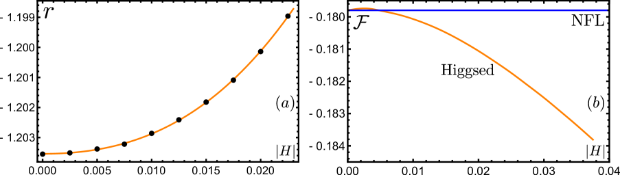
Figure 6: (a) Plot of $r$ as a function of $|H|$ in the higgsed phase, obtained from numerical solution of (55) in the $T\rightarrow 0$ limit. The orange line fits the numerical data with $r=r_{c}+h_{2}|H|^{2}+h_{3}|H|^{3}$, so $r-r_{c}\sim|H|^{2}$ as $|H|\rightarrow 0$. The values of parameters used are $t=t_{H}=g^{2}=g_{H}=1$, $2M=N$ and $\mu=0$. (b) Plot of the free energies per fermionic degree of freedom of the $|H|\neq 0$ solution (orange) and $H=0$ solution (blue) of (55). The weak first-order behavior at very small $|H|$ is due to a small finite $T=10^{-5}$ in the numerics, and disappears as $T\rightarrow 0$. The values of other parameters used are the same as in (a).

References

- Parcollet and Georges (1999) O. Parcollet and A. Georges, “Non-Fermi-liquid regime of a doped Mott insulator,” Phys. Rev. B 59, 5341 (1999), arXiv:cond-mat/9806119 .
- Gu et al. (2017) Y. Gu, A. Lucas, and X.-L. Qi, “Energy diffusion and the butterfly effect in inhomogeneous Sachdev-Ye-Kitaev chains,” SciPost Phys. 2, 018 (2017), arXiv:1702.08462 [hep-th] .
- Gu et al. (2017) Y. Gu, X.-L. Qi, and D. Stanford, “Local criticality, diffusion and chaos in generalized Sachdev-Ye-Kitaev models,” Journal of High Energy Physics 5, 125 (2017), arXiv:1609.07832 [hep-th] .
- Davison et al. (2017) R. A. Davison, W. Fu, A. Georges, Y. Gu, K. Jensen, and S. Sachdev, “Thermoelectric transport in disordered metals without quasiparticles: The Sachdev-Ye-Kitaev models and holography,” Phys. Rev. B 95, 155131 (2017), arXiv:1612.00849 [cond-mat.str-el] .
- Song et al. (2017) X.-Y. Song, C.-M. Jian, and L. Balents, “Strongly Correlated Metal Built from Sachdev-Ye-Kitaev Models,” Phys. Rev. Lett. 119, 216601 (2017), arXiv:1705.00117 [cond-mat.str-el] .
- Zhang (2017) P. Zhang, “Dispersive Sachdev-Ye-Kitaev model: Band structure and quantum chaos,” Phys. Rev. B 96, 205138 (2017), arXiv:1707.09589 [cond-mat.str-el] .
- Haldar et al. (2018) A. Haldar, S. Banerjee, and V. B. Shenoy, “Higher-dimensional Sachdev-Ye-Kitaev non-Fermi liquids at Lifshitz transitions,” Phys. Rev. B 97, 241106 (2018), arXiv:1710.00842 [cond-mat.str-el] .
- Ben-Zion and McGreevy (2018) D. Ben-Zion and J. McGreevy, “Strange metal from local quantum chaos,” Phys. Rev. B 97, 155117 (2018), arXiv:1711.02686 [cond-mat.str-el] .
- Patel et al. (2018a) A. A. Patel, J. McGreevy, D. P. Arovas, and S. Sachdev, “Magnetotransport in a Model of a Disordered Strange Metal,” Physical Review X 8, 021049 (2018a), arXiv:1712.05026 [cond-mat.str-el] .
- Chowdhury et al. (2018) D. Chowdhury, Y. Werman, E. Berg, and T. Senthil, “Translationally invariant non-Fermi liquid metals with critical Fermi-surfaces: Solvable models,” ArXiv e-prints (2018), arXiv:1801.06178 [cond-mat.str-el] .
- Fu et al. (2018) W. Fu, Y. Gu, S. Sachdev, and G. Tarnopolsky, “ fractionalized phases of a solvable, disordered, - model,” ArXiv e-prints (2018), arXiv:1804.04130 [cond-mat.str-el] .
- Sachdev and Ye (1993) S. Sachdev and J. Ye, “Gapless spin-fluid ground state in a random quantum Heisenberg magnet,” Physical Review Letters 70, 3339 (1993), cond-mat/9212030 .
- Kitaev (2015) A. Y. Kitaev, “Talks at KITP, University of California, Santa Barbara,” Entanglement in Strongly-Correlated Quantum Matter (2015).
- Sachdev (2015) S. Sachdev, “Bekenstein-Hawking Entropy and Strange Metals,” Physical Review X 5, 041025 (2015), arXiv:1506.05111 [hep-th] .
- Kitaev and Suh (2018) A. Kitaev and S. J. Suh, “The soft mode in the Sachdev-Ye-Kitaev model and its gravity dual,” JHEP 05, 183 (2018), arXiv:1711.08467 [hep-th] .
- Mitrano et al. (2018) M. Mitrano, A. A. Husain, S. Vig, A. Kogar, M. S. Rak, S. I. Rubeck, J. Schmalian, B. Uchoa, J. Schneeloch, R. Zhong, G. D. Gu, and P. Abbamonte, “Singular density fluctuations in the strange metal phase of a copper-oxide superconductor,” Proc. Nat. Acad. Sci. 115, 5392 (2018), arXiv:1708.01929 [cond-mat.str-el] .
- Cooper et al. (2009) R. A. Cooper, Y. Wang, B. Vignolle, O. J. Lipscombe, S. M. Hayden, Y. Tanabe, T. Adachi, Y. Koike, M. Nohara, H. Takagi, C. Proust, and N. E. Hussey, “Anomalous Criticality in the Electrical Resistivity of La2-xSrxCuO4,” Science 323, 603 (2009).
- Jin et al. (2011) K. Jin, N. P. Butch, K. Kirshenbaum, J. Paglione, and R. L. Greene, “Link between spin fluctuations and Cooper pairing in copper oxide superconductors,” Nature 476, 73 (2011), arXiv:1108.0940 [cond-mat.supr-con] .
- Legros et al. (2018) A. Legros, S. Benhabib, W. Tabis, F. Laliberté, M. Dion, M. Lizaire, B. Vignolle, D. Vignolles, H. Raffy, Z. Z. Li, P. Auban-Senzier, N. Doiron-Leyraud, P. Fournier, D. Colson, L. Taillefer, and C. Proust, “Universal -linear resistivity and Planckian limit in overdoped cuprates,” ArXiv e-prints (2018), arXiv:1805.02512 [cond-mat.supr-con] .
- Varma et al. (1989) C. M. Varma, P. B. Littlewood, S. Schmitt-Rink, E. Abrahams, and A. E. Ruckenstein, “Phenomenology of the normal state of Cu-O high-temperature superconductors,” Phys. Rev. Lett. 63, 1996 (1989).
- Faulkner et al. (2013) T. Faulkner, N. Iqbal, H. Liu, J. McGreevy, and D. Vegh, “Charge transport by holographic Fermi surfaces,” Phys. Rev. D 88, 045016 (2013), arXiv:1306.6396 [hep-th] .
- Cubrovic et al. (2009) M. Cubrovic, J. Zaanen, and K. Schalm, “String Theory, Quantum Phase Transitions and the Emergent Fermi-Liquid,” Science 325, 439 (2009), arXiv:0904.1993 [hep-th] .
- Sachdev (2010) S. Sachdev, “Holographic metals and the fractionalized Fermi liquid,” Phys. Rev. Lett. 105, 151602 (2010), arXiv:1006.3794 [hep-th] .
- Halperin et al. (1993) B. I. Halperin, P. A. Lee, and N. Read, “Theory of the half-filled Landau level,” Phys. Rev. B 47, 7312 (1993).
- Kaul et al. (2008) R. K. Kaul, Y. B. Kim, S. Sachdev, and T. Senthil, “Algebraic charge liquids,” Nature Physics 4, 28 (2008), arXiv:0706.2187 [cond-mat.str-el] .
- Sachdev et al. (2009) S. Sachdev, M. A. Metlitski, Y. Qi, and C. Xu, “Fluctuating spin density waves in metals,” Phys. Rev. B 80, 155129 (2009), arXiv:0907.3732 [cond-mat.str-el] .
- Chowdhury and Sachdev (2015) D. Chowdhury and S. Sachdev, “Higgs criticality in a two-dimensional metal,” Phys. Rev. B 91, 115123 (2015), arXiv:1412.1086 [cond-mat.str-el] .
- Sachdev and Chowdhury (2016) S. Sachdev and D. Chowdhury, “The novel metallic states of the cuprates: Fermi liquids with topological order and strange metals,” Progress of Theoretical and Experimental Physics 2016, 12C102 (2016), arXiv:1605.03579 [cond-mat.str-el] .
- Scheurer et al. (2018) M. S. Scheurer, S. Chatterjee, W. Wu, M. Ferrero, A. Georges, and S. Sachdev, “Topological order in the pseudogap metal,” Proc. Nat. Acad. Sci. 115, E3665 (2018), arXiv:1711.09925 [cond-mat.str-el] .
- Kim et al. (1994) Y. B. Kim, A. Furusaki, X.-G. Wen, and P. A. Lee, “Gauge-invariant response functions of fermions coupled to a gauge field,” Phys. Rev. B 50, 17917 (1994), cond-mat/9405083 .
- Patel (2018a) A. A. Patel, “gd.m,” Download imaginary-time code (2018a).
- Patel (2018b) A. A. Patel, “gdrealtime0.m,” Download real-time code (2018b).
- Georges et al. (2001) A. Georges, O. Parcollet, and S. Sachdev, “Quantum fluctuations of a nearly critical Heisenberg spin glass,” Phys. Rev. B 63, 134406 (2001), cond-mat/0009388 .
- (34) “Hypergeometric2F1,” Wolfram functions site .
- Sachdev (2018) S. Sachdev, “Topological order and Fermi surface reconstruction,” ArXiv e-prints (2018), arXiv:1801.01125 [cond-mat.str-el] .
- Lee (2018) S.-S. Lee, “Recent Developments in Non-Fermi Liquid Theory,” Annual Review of Condensed Matter Physics 9, 227 (2018), arXiv:1703.08172 [cond-mat.str-el] .
- Maldacena and Stanford (2016) J. Maldacena and D. Stanford, “Remarks on the Sachdev-Ye-Kitaev model,” Phys. Rev. D 94, 106002 (2016), arXiv:1604.07818 [hep-th] .
- Patel and Sachdev (2017) A. A. Patel and S. Sachdev, “Quantum chaos on a critical Fermi surface,” Proceedings of the National Academy of Science 114, 1844 (2017), arXiv:1611.00003 [cond-mat.str-el] .
- Fu and Sachdev (2016) W. Fu and S. Sachdev, “Numerical study of fermion and boson models with infinite-range random interactions,” Phys. Rev. B 94, 035135 (2016), arXiv:1603.05246 [cond-mat.str-el] .
- Patel et al. (2018b) A. A. Patel, M. J. Lawler, and E.-A. Kim, “Coherent superconductivity with large gap ratio from incoherent metals,” ArXiv e-prints (2018b), arXiv:1805.11098 [cond-mat.str-el] .
- Patel (2018c) A. A. Patel, “gdHiggs.m,” Download imaginary-time Higgs phase code (2018c).