Quantum Optimal Control for Mixed State Squeezing in Cavity Optomechanics

Abstract

The performance of key tasks in quantum technology, such as accurate state preparation, can be maximized by utilizing external controls and deriving their shape with optimal control theory. For non-pure target states, the performance measure needs to match both angle and length of the generalized Bloch vector. We introduce a measure based on this simple geometric picture that separates angle and length mismatch into individual terms and apply the ensuing optimization framework to maximize squeezing of an optomechanical oscillator at finite temperature. Our results show that shaping the cavity drives can speed up squeezed state preparation by more than two orders of magnitude. Cooperativities and pulse shapes required to this end are fully compatible with current experimental technology.

I Introduction

The ability to precisely control quantum systems is a prerequisite for harnessing quantum effects for quantum technology. Quantum optimal control provides a set of tools for deriving protocols to implement key tasks such as the preparation of non-classical states or the generation of entanglement Glaser et al. (2015). This approach can be used to determine, for example, the minimum time to carry out a given task with desired accuracy, even if the dynamics is not amenable to an analytical solution Caneva et al. (2009); Goerz et al. (2011); Sørensen et al. (2016). Recent examples include the fast and accurate preparation of a circular state, i.e., a Rydberg state with maximum projection angular momentum quantum number, for quantum sensing Patsch et al. (2018), and the determination of the fastest universal set of gates for quantum computing with superconducting transmon qubits Goerz et al. (2017).

Fast control protocols are particularly important for open quantum systems for which the interaction with the environment cannot be neglected Breuer and Petruccione (2002). An obvious control strategy is to ‘beat’ the decoherence resulting from the interaction with the environment. For quantum systems with Markovian, i.e., memoryless dynamics, this is often the only option Koch (2016). In contrast, strongly coupled environmental modes giving rise to significant system-environment correlations and non-Markovian dynamics are not necessarily detrimental but can also be exploited for control Basilewitsch et al. (2017); Reich et al. (2015).

An alternative approach to controlling open quantum systems consists in engineering driven dissipative dynamics in such a way that the desired target state becomes the steady state of the ensuing open system evolution Poyatos et al. (1996). This approach is particularly promising when the timescale of decoherence is comparable to or faster than that of the coherent evolution. Driven dissipative evolution is inherently robust against noise—a rather favorable feature in view of experimental implementation. In this context, preparation of non-classical states Krauter et al. (2011); Lin et al. (2013); Shankar et al. (2013); Kienzler et al. (2014); Kimchi-Schwartz et al. (2016) and generation of non-equilibrium quantum phases Syassen et al. (2008); Schindler et al. (2013) have successfully been demonstrated with trapped atoms and ions as well as superconducting qubits. For the example of trapped ions, determining the key parameters of the driven dissipative dynamics by quantum optimal control is predicted to allow reaching the fundamental performance limits Horn et al. (2018).

Another platform ideally suited for implementing driven dissipative dynamics is cavity optomechanics Aspelmeyer et al. (2014a, b), where a mechanical resonator is coupled to an optical or microwave cavity. Optomechanical systems are promising candidates for quantum-enhanced sensing, coherent light-matter interfaces, and fundamental tests of quantum mechanics. In particular, the cavity drive can be employed to generate arbitrary quantum states of the mechanical oscillator Aspelmeyer et al. (2014a), including strongly squeezed states. These states are useful in applications such as quantum information processing Yonezawa and Furusawa (2010), atomic clocks Leroux et al. (2010) or, most prominently, quantum-enhanced sensing Schnabel (2017); Hosten et al. (2016) where they allow to increase sensitivity of e.g. gravitational wave detectors Aasi et al. (2013); Grote et al. (2013). Squeezed states can be generated in various physical platforms Andersen et al. (2016). In cavity optomechanics, driven-dissipative evolution can be used to produce substantially squeezed states Kronwald et al. (2013); Wollman et al. (2015). While preparation of the mechanical resonator in a pure quantum state remains a major goal of cavity optomechanics, interesting non-classical states can be realized also at finite temperature Palomaki et al. (2013); Wollman et al. (2015); Pirkkalainen et al. (2015). This is true in particular for squeezed states since there is a trade off between squeezing strength and purity.

Cavity drives for state preparation in cavity optomechanics are typically taken to have constant amplitude Aspelmeyer et al. (2014a). On the other hand, pulsed excitation has recently been shown to allow for probing the resonator state with minimal heating Meenehan et al. (2015). This raises the question whether explicitly time-dependent amplitudes of the cavity drives can also be used to improve state preparation protocols. Here, we specifically ask by how much, at a given non-zero temperature, suitable pulse shapes can speed up the preparation of the mechanical oscillator in a squeezed state.

To derive the pulse shape of the cavity drives, we employ optimal control theory which needs to target a mixed steady state, due to finite temperature. Standard optimization functionals, defined originally for pure target states, cannot be used in this case; and alternative formulations using, e.g., the Hilbert-Schmidt distance need to be employed Xu et al. (2004). We give an intuitive, geometrical explanation for the failure of the standard functionals by visualizing the dynamics on the generalized Bloch sphere. This picture is also useful to elucidate the requirements an optimization functional targeting mixed states need to fulfill. Using this geometric interpretation, we furthermore refine the functional based on the Hilbert-Schmidt distance Xu et al. (2004) to one that seeks to match the target state’s Bloch vector angle and length separately. We employ both functionals to optimize the preparation of a mechanical resonator in a squeezed state and compare their performance.

The paper is organized as follows. The framework of quantum optimal control theory is presented in Sec. II. In Sec. II.1 we briefly review Krotov’s method Krotov (1995), our optimization algorithm of choice, in Sec. II.2 we illustrate the failure of standard functionals, and in Sec. II.3 we construct target functionals based on Bloch vector angle and length. Section III is dedicated to the application of this methodology to preparing a squeezed state at finite temperature in cavity optomechanics. We introduce the model and control problem in Sec. III.1, present our results in Sec. III.2 and discuss the performance of various target functionals in Sec. III.3. Finally, Sec. IV concludes.

II Quantum Optimal Control Theory

Quantum control assumes that the dynamics of a quantum system can be steered, typically by a set of external driving fields $\left\{\mathcal{E}_{k}(t)\right\}$. How to choose the external drives in the best possible way is the subject of quantum optimal control theory (OCT) Glaser et al. (2015). Optimality is sought using an optimization functional,

$$J\left[\left\{\mathcal{E}_{k}\right\},\left\{\mathsf{\hat{\rho}}_{l}\right\}\right] =D\left[\left\{\mathsf{\hat{\rho}}_{l}(T)\right\}\right]$$ (1)

$$\quad+\int_{0}^{T}\mathrm{d}t\,g\left[\left\{\mathcal{E}_{k}(t)\right\},\left\{\mathsf{\hat{\rho}}_{l}(t)\right\},t\right],$$

where $\left\{\mathsf{\hat{\rho}}_{l}(t)\right\}$ is a set of forward propagated states, $D\left[\left\{\mathsf{\hat{\rho}}_{l}(T)\right\}\right]$ is the figure or merit at final time $T$ and $g$ captures additional costs or constraints at intermediate times, for instance by restricting the field spectra or by penalizing population in certain subspaces.

A control problem is tackled by choosing (i) an appropriate optimization functional $J$ and (ii) an appropriate method to minimize $J$. While $J$ captures the physics of the problem, the choice of the method is relevant as well, since it often determines whether a solution can be found in practice. Gradient-based techniques hold the promise of faster convergence than gradient-free methods Glaser et al. (2015). However, they require the ability to determine the derivatives of the functional with respect to the states. Whether this is feasible or not depends on the choice of the functional. In the following, we focus on Krotov’s method Krotov (1995); Konnov and Krotov (1999), a gradient-based algorithm, but our considerations are valid for any gradient-based method requiring functional derivatives.

The general idea of any gradient-based method is to find an extremum of the total functional (1) using gradient information with respect to changes in the control fields $\{\mathcal{E}_{k}(t)\}$. The extremum condition together with the requirement to fulfill the dynamical equations leads to two equations of motion - one for the states $\left\{\mathsf{\hat{\rho}}_{l}(t)\right\}$ and one for the so-called co-states $\{\mathsf{\hat{\chi}}_{l}(t)\}$. While the former corresponds to the usual forward propagation in time starting at the initial condition $\left\{\mathsf{\hat{\rho}}_{l}(0)\right\}$, the latter can be interpreted as a backward propagation in time, starting at $\{\mathsf{\hat{\chi}}_{l}(T)\}$. This “initial” condition for the backward propagation contains information about the physical final time target encoded by the functional $D$. The optimization algorithms then tries to match both forward and backward propagated states, thus ensuring approach towards the target $\left\{\mathsf{\hat{\rho}}_{l}(T)\right\}$ at final time, which in turn minimizes functional (1).

II.1 Gradient-based optimization with Krotov’s method

Krotov’s method Krotov (1995); Konnov and Krotov (1999) is a sequential optimization technique with built-in monotonic convergence. A possible choice of the functional $g$ is Palao and Kosloff (2003)

$$g\left[\left\{\mathcal{E}_{k}(t)\right\}\right]=\sum_{k}\frac{\lambda_{k}}{S_{k}(t)}\left(\mathcal{E}_{k}(t)-\mathcal{E}_{k}^{\mathrm{ref}}(t)\right)^{2},$$ (2)

where $\mathcal{E}_{k}^{\mathrm{ref}}(t)$ is a reference field (taken to be the field from the last iteration), $S_{k}(t)\in(0,1]$ a shape function to smoothly switch $\mathcal{E}_{k}(t)$ on and off, and $\lambda_{k}$ a parameter that controls the step size. Using Eq. (2), the update equation for the field $\mathcal{E}_{k}(t)$ becomes Reich et al. (2012); Goerz et al. (2014)

$$\mathcal{E}_{k}^{(i+1)}(t)=\mathcal{E}_{k}^{\mathrm{ref}}(t)+\frac{S_{k}(t)}{\lambda_{k}}\mathfrak{Im}\left\{\sum_{l}\Braket{\mathsf{\hat{\chi}}^{(i)}_{l}(t)\;,\;\frac{\partial\mathcal{L}\left[\left\{\mathcal{E}_{k^{\prime}}\right\}\right]}{\partial\mathcal{E}_{k}}\Big{missing}}{{}_{\{\mathcal{E}^{(i+1)}_{k^{\prime}}(t)\}}\mathsf{\hat{\rho}}^{(i+1)}_{l}(t)}\right\},$$ (3)

where $\braket{\mathsf{\hat{A}},\mathsf{\hat{B}}}\equiv\mathrm{Tr}\{\mathsf{\hat{A}}^{\dagger}\mathsf{\hat{B}}\}$ is the Hilbert-Schmidt overlap and $\mathcal{L}\left[\left\{\mathcal{E}_{k}\right\}\right]$ the field-dependent generator of the dynamics, e.g. the Liouvillian of a Lindblad master equation Breuer and Petruccione (2002). $\{\mathsf{\hat{\rho}}^{(i+1)}_{l}(t)\}$ are forward propagated states,

$$\frac{\mathrm{d}}{\mathrm{d}t}\mathsf{\hat{\rho}}^{(i+1)}_{l}(t)=-\frac{\textup{i}}{\hbar}\mathcal{L}\left[\left\{\mathcal{E}^{(i+1)}_{k}\right\}\right]\mathsf{\hat{\rho}}^{(i+1)}_{l}(t)\,,$$ (4a)

with initial conditions

$$\mathsf{\hat{\rho}}^{(i+1)}_{l}(0)=\mathsf{\hat{\rho}}_{l}(0)\,,$$ (4b)

whereas the co-states $\{\mathsf{\hat{\chi}}^{(i)}_{l}(t)\}$ are solutions of the adjoint equation of motion,

$$\frac{\mathrm{d}}{\mathrm{d}t}\mathsf{\hat{\chi}}^{(i)}_{l}(t)=\frac{\textup{i}}{\hbar}\mathcal{L}^{\dagger}\left[\left\{\mathcal{E}^{(i)}_{k}\right\}\right]\mathsf{\hat{\chi}}^{(i)}_{l}(t)\,,$$ (5a)

and their ‘initial’ condition (at final time $$T$$) is determined by the target functional,

$$\mathsf{\hat{\chi}}^{(i)}_{l}(T)=-\nabla_{\mathsf{\hat{\rho}}_{l}(T)}D\big{|}_{\{\mathsf{\hat{\rho}}^{(i)}_{l^{\prime}}(T)\}}\,.$$ (5b)

The superscripts $(i+1)$ and $(i)$ in Eqs. (3)-(5) indicate the current and previous iteration in the optimization procedure, respectively. The choice of $D\left[\left\{\mathsf{\hat{\rho}}_{l}(T)\right\}\right]$ enters via Eq. (5b), where the derivative of functional $D$ with respect to $\mathsf{\hat{\rho}}_{l}(T)$ needs to be evaluated. For a detailed derivation of Krotov’s method in the context of quantum control see Ref. Reich et al. (2012).

II.2 Failure of overlap-based functionals for mixed state targets

State transfers, where a set of initial states $\left\{\mathsf{\hat{\rho}}_{l}(0)\right\}$ must simultaneously be transferred into a set of target states $\left\{\mathsf{\hat{\rho}}_{l}^{\mathrm{trg}}\right\}$, represent a standard control problem. Solving this problem requires a reliable measure $D(\mathsf{\hat{\rho}}_{l}(T),\mathsf{\hat{\rho}}_{l}^{\mathrm{trg}})$ for the state distance between forward propagated state $\mathsf{\hat{\rho}}_{l}(T)$ and target $\mathsf{\hat{\rho}}_{l}^{\mathrm{trg}}$. For two pure states $\Psi_{1},\Psi_{2}$, a standard choice is Palao and Kosloff (2003)

$$D_{\mathrm{re}}\left(\Psi_{1},\Psi_{2}\right) =1-\mathfrak{Re}\left\{\tau\right\},\quad\text{or}$$ (6a)

$$D_{\mathrm{sm}}\left(\Psi_{1},\Psi_{2}\right) =1-\left|\tau\right|^{2},$$ (6b)

where $\tau=\Braket{\Psi_{1}}{\Psi_{2}}\in\mathbb{C}$, $|\tau|\leq 1$, is the complex overlap in Hilbert space. Both functionals rely on $\tau$ to serve as a distance measure in state space, and any OCT algorithm that minimizes $D_{\mathrm{re}}$ or $D_{\mathrm{sm}}$ necessarily maximizes $\mathfrak{Re}\left\{\tau\right\}$ or $|\tau|$, respectively. Equations (6) cannot, however, simply be generalized to non-pure states. For density matrices $\mathsf{\hat{\rho}}_{1}$, $\mathsf{\hat{\rho}}_{2}$, the overlap in Liouville space, $\tau=\braket{\mathsf{\hat{\rho}}_{1},\mathsf{\hat{\rho}}_{2}}\in\mathbb{R}$, defined in terms of the Hilbert-Schmidt overlap, becomes real, and minimizing $D_{\mathrm{re}}$, $D_{\mathrm{sm}}$ implies maximizing $\tau$. Unfortunately, $\tau$ is no longer a reliable measure for closeness once $\mathsf{\hat{\rho}}_{1},\mathsf{\hat{\rho}}_{2}$ are both mixed.

We illustrate the problem with the simplest example of a quantum system, a qubit. Representing the qubit state in the canonical basis, $\left\{\Ket{0},\Ket{1}\right\}$, consider

$$\mathsf{\hat{\rho}}(\alpha)=\begin{pmatrix}\alpha&0\\ 0&1-\alpha\end{pmatrix}\,,\qquad\mathsf{\hat{\rho}}^{\mathrm{trg}}=\begin{pmatrix}\beta&0\\ 0&1-\beta\end{pmatrix}\,,$$ (7)

where $0\leq\alpha$, $\beta\leq 1$. Both states are equivalent iff $\alpha=\beta$ and $\tau_{\mathrm{trg}}\equiv\Braket{\mathsf{\hat{\rho}}(\beta),\mathsf{\hat{\rho}}^{\mathrm{trg}}}=\beta^{2}+(1-\beta)^{2}$. However, for pure states such as $\mathsf{\hat{\rho}}(1)$ or $\mathsf{\hat{\rho}}(0)$, $\tau=\beta$ or $\tau=1-\beta$. This results in $\tau>\tau_{\mathrm{trg}}$ for $\beta\in(\frac{1}{2},1)$ or $\beta\in(0,\frac{1}{2})$, respectively. Thus, pure states maximize $\tau$ and thus the figure of merit (6) despite being obviously different from the target $\mathsf{\hat{\rho}}^{\mathrm{trg}}$. Moreover, for the completely mixed state $\mathsf{\hat{\rho}}^{\mathrm{trg}}=\mathrm{diag}\{0.5,0.5\}$, we find $\tau=\braket{\mathsf{\hat{\rho}}(\alpha),\mathsf{\hat{\rho}}^{\mathrm{trg}}}=\frac{1}{2}$ for all $\alpha$. In this case, $\tau$ is not even able to indicate differences at all.

Figure 1: Optimization results for a qubit, where the dynamics is governed by Eq. (8). The initial state is $\mathsf{\hat{\rho}}(0)=\Ket{1}\Bra{1}$, the target state $\mathsf{\hat{\rho}}^{\mathrm{trg}}=\mathrm{diag}\{0.6,0.4\}$ and the initial field $u(t)=0.01$ with total propagation time $T=1$. (a) Final-time functionals $D_{\mathrm{re}}$ and $D_{\mathrm{sm}}$, cf. Eq. (6), as a function of the number of iterations. (b) Population $\alpha(T)$ in $\Ket{0}$ at final time. The horizontal line indicates the respective population of the target state $\mathsf{\hat{\rho}}^{\mathrm{trg}}$. (c) Trace distance $D_{\mathrm{tr}}$, cf. Eq. (11), between propagated state $\mathsf{\hat{\rho}}(T)$ and target state $\mathsf{\hat{\rho}}^{\mathrm{trg}}$.

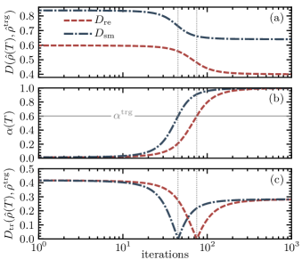
The ill-definedness of the overlap-based functionals (6) in case of mixed target states is easily demonstrated by a toy control problem. Consider a qubit whose dynamics is determined by a purely dissipative master equation Breuer and Petruccione (2002),

$$\textup{i}\hbar\frac{\mathrm{d}}{\mathrm{d}t}\mathsf{\hat{\rho}}(t) =\mathcal{L}\left[u(t)\right]\mathsf{\hat{\rho}}(t)$$ (8)

$$=\textup{i}\hbar u(t)\left[\mathsf{\hat{\sigma}}_{-}\mathsf{\hat{\rho}}(t)\mathsf{\hat{\sigma}}_{+}-\frac{1}{2}\left\{\mathsf{\hat{\sigma}}_{+}\mathsf{\hat{\sigma}}_{-},\mathsf{\hat{\rho}}(t)\right\}\right],$$

where $\mathsf{\hat{\sigma}}_{-}(\mathsf{\hat{\sigma}}_{+})$ are the standard lowering (raising) operators and $u(t)\geq 0$ is a time-dependent, controllable decay rate. We choose the initial state of the qubit to be $\mathsf{\hat{\rho}}(0)=\Ket{1}\Bra{1}$. Thus, we can reach any diagonal state $\mathsf{\hat{\rho}}(T)=\alpha(T)\Ket{0}\Bra{0}+(1-\alpha(T))\Ket{1}\Bra{1}$ with $\alpha(T)>0$, since $\alpha(T)$ can be controlled by appropriately choosing $u(t)$ for $t\in[0,T]$. Figure 1 presents optimization results for a mixed state target, $\mathsf{\hat{\rho}}^{\mathrm{trg}}=0.6\Ket{0}\Bra{0}+0.4\Ket{1}\Bra{1}$, employing the functionals (6). Figure 1(a) shows the monotonic decrease of both functionals over the number of iterations, as expected for Krotov’s method, while Fig. 1(b) plots the corresponding final time ground state population $\alpha(T)$. The optimization starts with a fairly low ground state population, $\alpha(T)\sim 0$, due to the non-optimal, i.e., too small, guess field $u(t)$. The decay rate is increased during optimization such that $\alpha(T)\sim 1$ after convergence is reached. This result maximizes the overlap since $\tau_{\mathrm{opt}}\equiv\Braket{\mathsf{\hat{\rho}}_{\mathrm{opt}}(T),\mathsf{\hat{\rho}}^{\mathrm{trg}}}>\Braket{\mathsf{\hat{\rho}}^{\mathrm{trg}},\mathsf{\hat{\rho}}^{\mathrm{trg}}}\equiv\tau_{\mathrm{eq}}$ with $\mathsf{\hat{\rho}}_{\mathrm{opt}}(T)=\Ket{0}\Bra{0}$, and thus realizes smaller values of the functionals $D_{\mathrm{re}}$ and $D_{\mathrm{sm}}$. However, this is not what the optimization is supposed to achieve. Figure 1(c) shows the trace distance $D_{\mathrm{tr}}$ (a reliable measure for the closeness of states, as we will discuss in Sec. II.3) between $\mathsf{\hat{\rho}}(T)$ and $\mathsf{\hat{\rho}}^{\mathrm{trg}}$ as a function of the number of iterations. A minimum is observed at the correct value $\alpha(T)=\alpha^{\mathrm{trg}}=0.6$. The increase of $D_{\mathrm{tr}}$ as the iterative algorithm proceeds, which is due to further minimization of $D_{\mathrm{re}}$ and $D_{\mathrm{sm}}$, illustrates that the optimization misses the desired target.

This observation can be fully generalized to $N$-level systems with a simple geometric picture Bertlmann and Krammer (2008). By choosing a basis of traceless, Hermitian $N\times N$ matrices, $\{\mathsf{\hat{A}}_{i}\}$, with $\braket{\mathsf{\hat{A}}_{i},\mathsf{\hat{A}}_{j}}=\delta_{i,j}$, we can write $\mathsf{\hat{\rho}}$ as

$$\mathsf{\hat{\rho}}=\frac{1}{N}\mathsf{\hat{\mathbbm{1}}}_{N}+\boldsymbol{r}\cdot\boldsymbol{\mathsf{\hat{A}}}\,,$$ (9)

where $\boldsymbol{r}=(a_{1},a_{2},\dots)^{\top}$ is the generalized Bloch vector, containing the expansion coefficients for matrices $\boldsymbol{\mathsf{\hat{A}}}=(\mathsf{\hat{A}}_{1},\mathsf{\hat{A}}_{2},\dots)^{\top}$. Then, the Hilbert-Schmidt overlap of two states $\mathsf{\hat{\rho}}_{1},\mathsf{\hat{\rho}}_{2}$ becomes

$$\tau=\Braket{\mathsf{\hat{\rho}}_{1},\mathsf{\hat{\rho}}_{2}}=\frac{1}{N}+\boldsymbol{r}_{1}\cdot\boldsymbol{r}_{2}=\frac{1}{N}+\left|\boldsymbol{r}_{1}\right|\left|\boldsymbol{r}_{2}\right|\cos(\theta)\,,$$ (10)

where $|\boldsymbol{r}_{1}|,|\boldsymbol{r}_{2}|$ are the lengths of the respective Bloch vectors and $\theta$ is the angle between them. Hence, maximization of $\tau$ means maximizing $|\boldsymbol{r}_{1}|,|\boldsymbol{r}_{2}|$ and minimizing $\theta$.

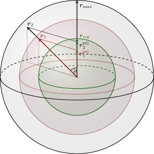
Figure 2 illustrates the behavior of the overlap geometrically, comparing two states $\mathsf{\hat{\rho}}_{1},\mathsf{\hat{\rho}}_{2}$ with Bloch vectors $\boldsymbol{r}_{1},\boldsymbol{r}_{2}$ to the target state $\mathsf{\hat{\rho}}_{\mathrm{trg}}$ with $\boldsymbol{r}_{\mathrm{trg}}$. Here, we assume $\boldsymbol{r}_{1}\parallel\boldsymbol{r}_{2}$ and $|\boldsymbol{r}_{2}|>|\boldsymbol{r}_{1}|>|\boldsymbol{r}_{\mathrm{trg}}|$. In this case, the angles $\theta_{1}$, $\theta_{2}$ of $\boldsymbol{r}_{1}$ and $\boldsymbol{r}_{2}$ with $\boldsymbol{r}_{\mathrm{trg}}$ are identical but the purer state $\boldsymbol{r}_{2}$ has the larger projection onto $\boldsymbol{r}_{\mathrm{trg}}$ and thus yields $\tau_{2}\equiv\braket{\mathsf{\hat{\rho}}_{2},\mathsf{\hat{\rho}}^{\mathrm{trg}}}>\braket{\mathsf{\hat{\rho}}_{1},\mathsf{\hat{\rho}}^{\mathrm{trg}}}\equiv\tau_{1}$. This contradicts the expectation that $\mathsf{\hat{\rho}}_{2}$ should be further away from $\mathsf{\hat{\rho}}^{\mathrm{trg}}$ than $\mathsf{\hat{\rho}}_{1}$—a fact that is evidently not captured by the functionals (6). Moreover, the simple geometric picture of Fig. 2 demonstrates that the state maximizing $\tau$ is always the pure state $\mathsf{\hat{\rho}}_{\mathrm{max}}$ with $\boldsymbol{r}_{\mathrm{max}}\parallel\boldsymbol{r}_{\mathrm{trg}}$ and $\theta=0$. This readily explains the optimization results of Fig. 1.

Figure 2: Bloch vectors $\boldsymbol{r}_{1},\boldsymbol{r}_{2},\boldsymbol{r}_{\mathrm{trg}},\boldsymbol{r}_{\mathrm{max}}$ in a generalized Bloch sphere. The outer sphere indicates pure states while the inner spheres correspond to mixed states. $\boldsymbol{r}_{1}^{\mathrm{prj}},\boldsymbol{r}_{2}^{\mathrm{prj}}$ are the projections of $\boldsymbol{r}_{1},\boldsymbol{r}_{2}$ onto $\boldsymbol{r}_{\mathrm{trg}}$.

II.3 A Bloch vector-based functional for mixed state targets

Before inspecting specific measures for the closeness of two mixed states to replace an overlap-based functional (6), we summarize the desirable properties that a distance measure should satisfy for use in OCT. Let $S_{\mathcal{H}}$ be the space of density matrices over the Hilbert space $\mathcal{H}$. A function $D$, which quantifies the distance of two states $\mathsf{\hat{\rho}}_{1},\mathsf{\hat{\rho}}_{2}\in S_{\mathcal{H}}$, should fulfill

1. $\forall\mathsf{\hat{\rho}}_{1},\mathsf{\hat{\rho}}_{2}\in S_{\mathcal{H}}:D\left(\mathsf{\hat{\rho}}_{1},\mathsf{\hat{\rho}}_{2}\right)\in\mathbb{R}$ ,

2. $D\left(\mathsf{\hat{\rho}}_{1},\mathsf{\hat{\rho}}_{2}\right)=\underset{\mathsf{\hat{\rho}}_{1}^{\prime},\mathsf{\hat{\rho}}_{2}^{\prime}\in S_{\mathcal{H}}}{\mathrm{inf}}D\left(\mathsf{\hat{\rho}}_{1}^{\prime},\mathsf{\hat{\rho}}_{2}^{\prime}\right)\quad\Leftrightarrow\quad\mathsf{\hat{\rho}}_{1}=\mathsf{\hat{\rho}}_{2}$ .

These two conditions provide the minimal framework for suitable state-to-state optimization functionals. The first property ensures that an order relation can be established. This is essential since it allows the optimization algorithm to quantify improvement in terms of a decrease of the function value. The second property guarantees that the minimal value identifies the desired state uniquely .

Evidently, the second property is not met by the overlap-based functionals $D_{\mathrm{re}}$ and $D_{\mathrm{sm}}$. However, there exist various distance measures satisfying the two properties Gilchrist et al. (2005); Dajka et al. (2011), for instance, the trace distance Nielsen and Chuang (2011),

$$D_{\mathrm{tr}}\left(\mathsf{\hat{\rho}}_{1},\mathsf{\hat{\rho}}_{2}\right)=\frac{1}{2}\left\lVert\mathsf{\hat{\rho}}_{1}-\mathsf{\hat{\rho}}_{2}\right\rVert_{\mathrm{tr}}\,,\;\left\lVert\mathsf{\hat{\rho}}\right\rVert_{\mathrm{tr}}=\mathrm{Tr}\left\{\sqrt{\mathsf{\hat{\rho}}^{\dagger}\mathsf{\hat{\rho}}}\right\}\,,$$ (11)

the Bures distance, based on the Uhlmann fidelity Uhlmann (1976); Jozsa (1994),

$$D_{\mathrm{Bures}}\left(\mathsf{\hat{\rho}}_{1},\mathsf{\hat{\rho}}_{2}\right)=\sqrt{1-\mathrm{Tr}\left\{\sqrt{\sqrt{\mathsf{\hat{\rho}}_{1}}\mathsf{\hat{\rho}}_{2}\sqrt{\mathsf{\hat{\rho}}_{1}}}\right\}},$$ (12)

the Hellinger distance Luo and Zhang (2004),

$$D_{\mathrm{Hellinger}}\left(\mathsf{\hat{\rho}}_{1},\mathsf{\hat{\rho}}_{2}\right)=\sqrt{1-\mathrm{Tr}\left\{\sqrt{\mathsf{\hat{\rho}}_{1}}\sqrt{\mathsf{\hat{\rho}}_{2}}\right\}},$$ (13)

the Jensen-Shannon divergence Majtey et al. (2005),

$$D_{\mathrm{JS}}\left(\mathsf{\hat{\rho}}_{1},\mathsf{\hat{\rho}}_{2}\right)=\sqrt{E\left(\frac{\mathsf{\hat{\rho}}_{1}+\mathsf{\hat{\rho}}_{2}}{2}\right)-\frac{1}{2}E\left(\mathsf{\hat{\rho}}_{1}\right)-\frac{1}{2}E\left(\mathsf{\hat{\rho}}_{2}\right)},$$ (14)

with $E(\mathsf{\hat{\rho}})=\mathrm{Tr}\{\mathsf{\hat{\rho}}\,\mathrm{ln}\left(\mathsf{\hat{\rho}}\right)\}$ the von Neumann entropy Bennett et al. (1996), and the Hilbert-Schmidt distance Dodonov et al. (2000),

$$D_{\mathrm{HS}}\left(\mathsf{\hat{\rho}}_{1},\mathsf{\hat{\rho}}_{2}\right) =\frac{1}{2}\mathrm{Tr}\left\{\left(\mathsf{\hat{\rho}}_{1}-\mathsf{\hat{\rho}}_{2}\right)^{2}\right\},$$ (15)

to name just a few. Note that $D_{\mathrm{HS}}$ appears in a slightly modified version to match the definition in Ref. Xu et al. (2004), and some of the other measures have been adapted to satisfy $D\in[0,1]$. Although measures (11)-(15) fulfill the two properties, there is still one caveat left: With regard to gradient-based optimization almost all of them suffer from the fact that no closed analytical expression for their derivatives with respect to $\mathsf{\hat{\rho}}_{1}$ or $\mathsf{\hat{\rho}}_{2}$ exists. When resorting to numerical evaluation of the derivatives, the required spectral decomposition results in accuracy problems due to the presence of square roots, respectively logarithms, of the state. This problem becomes particularly severe in the common case that several eigenvalues of the density matrix are close to zero, rendering most of the aforementioned functionals impractical for application in gradient-based optimization.

A notable exception is the Hilbert-Schmidt distance (15), which therefore has already found use in gradient-based OCT Xu et al. (2004). Motivated by the simple geometric picture of state mismatch, cf. Fig. 2, one can also easily understand, why $D_{\mathrm{HS}}$, in contrast to $D_{\mathrm{re}}$ or $D_{\mathrm{sm}}$, is reliable. In terms of Bloch vectors, it reads

$$D_{\mathrm{HS}}\left(\mathsf{\hat{\rho}}_{1},\mathsf{\hat{\rho}}_{2}\right) =\frac{1}{2}\lvert\boldsymbol{r}_{1}-\boldsymbol{r}_{2}\rvert^{2},$$ (16)

where $D_{\mathrm{HS}}=0$ is only attainable in case of identical Bloch vectors.

While the Hilbert-Schmidt distance mixes “angle” and “length” mismatch in a single term, one might wonder whether splitting up both contributions into two separate terms, say $D_{\mathrm{angle}}$ and $D_{\mathrm{length}}$, allows for a more targeted optimization. We therefore define

$$D_{\mathrm{split}}\left(\mathsf{\hat{\rho}}_{1},\mathsf{\hat{\rho}}_{2}\right) =\alpha_{1}D_{\mathrm{angle}}\left(\mathsf{\hat{\rho}}_{1},\mathsf{\hat{\rho}}_{2}\right)+\alpha_{2}D_{\mathrm{length}}\left(\mathsf{\hat{\rho}}_{1},\mathsf{\hat{\rho}}_{2}\right),$$ (17)

where $\alpha_{1},\alpha_{2}\geq 0$ are numerical parameters that allow to weight the contributions individually, and

$$D_{\mathrm{angle}}\left(\mathsf{\hat{\rho}}_{1},\mathsf{\hat{\rho}}_{2}\right) =\frac{1}{\pi^{2}}\arccos^{2}\left(\frac{d_{12}}{\sqrt{d_{11}d_{22}}}\right)\,,$$ (18a)

$$D_{\mathrm{length}}\left(\mathsf{\hat{\rho}}_{1},\mathsf{\hat{\rho}}_{2}\right) =\frac{N}{N-1}\left(\sqrt{d_{11}}-\sqrt{d_{22}}\right)^{2}\,,$$ (18b)

where we have used $d_{ij}\equiv\Braket{\mathsf{\hat{\rho}}_{i},\mathsf{\hat{\rho}}_{j}}-1/N=\boldsymbol{r}_{i}\cdot\boldsymbol{r}_{j}$. In the Bloch representation, we find the simpler form

$$D_{\mathrm{angle}}\left(\mathsf{\hat{\rho}}_{1},\mathsf{\hat{\rho}}_{2}\right) =\frac{\theta^{2}}{\pi^{2}}\,,$$ (19a)

$$D_{\mathrm{length}}\left(\mathsf{\hat{\rho}}_{1},\mathsf{\hat{\rho}}_{2}\right) =\frac{N}{N-1}\Big{(}\left|\boldsymbol{r}_{1}\right|-\left|\boldsymbol{r}_{2}\right|\Big{)}^{2}\,,$$ (19b)

from which it is clear that both terms quantify angle and length mismatch individually. Measure (17) fulfills all required properties and can easily be derived with respect to $\mathsf{\hat{\rho}}_{1}$ and $\mathsf{\hat{\rho}}_{2}$. The derivatives read 

$$\nabla_{\mathsf{\hat{\rho}}_{1}}D_{\mathrm{angle}}\left(\mathsf{\hat{\rho}}_{1},\mathsf{\hat{\rho}}_{2}\right) =-\frac{2}{\pi^{2}}\arccos\left(\frac{d_{12}}{\sqrt{d_{11}d_{22}}}\right)$$

$$\quad\times\frac{\mathsf{\hat{\rho}}_{2}-\frac{d_{12}}{d_{11}}\mathsf{\hat{\rho}}_{1}}{\sqrt{d_{11}d_{22}-d_{12}^{2}}}\,,$$ (20a)

$$\nabla_{\mathsf{\hat{\rho}}_{1}}D_{\mathrm{length}}\left(\mathsf{\hat{\rho}}_{1},\mathsf{\hat{\rho}}_{2}\right) =2\frac{N}{N-1}\frac{\sqrt{d_{11}}-\sqrt{d_{22}}}{\sqrt{d_{11}}}\mathsf{\hat{\rho}}_{1}\,.$$ (20b)

III Application: Generation of Mixed State Squeezing

III.1 Model and Control Problem

We follow Ref. Kronwald et al. (2013) and consider a mode of an optical cavity and one of a mechanical resonator, coupled via radiation pressure. The optical cavity is driven by two lasers at the mechanical sidebands, $\omega_{\pm}=\omega_{\mathrm{cav}}\pm\Omega$, where $\omega_{\mathrm{cav}}$ and $\Omega$ are the frequencies of cavity and mechanical resonator, respectively. In the linearized regime, the Hamiltonian describing the joint system of cavity and resonator reads Kronwald et al. (2013)

$$\mathsf{\hat{H}} =-\hbar\mathsf{\hat{d}}^{\dagger}\left(G_{+}\mathsf{\hat{b}}^{\dagger}+G_{-}\mathsf{\hat{b}}\right)+\mathrm{H.c.}$$ (21)

$$\quad-\hbar\mathsf{\hat{d}}^{\dagger}\left(G_{+}\mathsf{\hat{b}}e^{-2\textup{i}\Omega t}+G_{-}\mathsf{\hat{b}}^{\dagger}e^{2\textup{i}\Omega t}\right)+\mathrm{H.c.}\,,$$

where $\mathsf{\hat{d}}$ ($\mathsf{\hat{b}}$) are the annihilation operators for photons (phonons). $G_{+}$ ($G_{-}$) are effective optomechanical coupling rates, given by the optomechanical coupling constant times the amplitude of the lasers driving the blue (red) sideband of the cavity. To account for decay, we use the quantum optical master equation Breuer and Petruccione (2002),

$$\textup{i}\hbar\frac{\mathrm{d}}{\mathrm{d}t}\mathsf{\hat{\rho}}(t) =\mathcal{L}\mathsf{\hat{\rho}}(t)$$ (22)

$$=\left[\mathsf{\hat{H}},\mathsf{\hat{\rho}}(t)\right]+\textup{i}\hbar\sum_{l=1}^{3}\Big{(}\mathsf{\hat{L}}_{l}\mathsf{\hat{\rho}}(t)\mathsf{\hat{L}}_{l}^{\dagger}-\frac{1}{2}\big{\{}\mathsf{\hat{L}}_{l}^{\dagger}\mathsf{\hat{L}}_{l},\mathsf{\hat{\rho}}(t)\big{\}}\Big{)}\,,$$

to describe the system’s dynamics. The Lindblad operators are given by

$$\mathsf{\hat{L}}_{1} =\sqrt{\kappa}\,\mathsf{\hat{d}}\,,$$ (23a)

$$\mathsf{\hat{L}}_{2} =\sqrt{\Gamma_{M}\left(n_{\mathrm{th}}+1\right)}\,\mathsf{\hat{b}}\,,$$ (23b)

$$\mathsf{\hat{L}}_{3} =\sqrt{\Gamma_{M}n_{\mathrm{th}}}\,\mathsf{\hat{b}}^{\dagger}$$ (23c)

with $\kappa$ and $\Gamma_{M}$ the photon and phonon decay rates, respectively, and $n_{\mathrm{th}}$ describing the thermal occupancy of the mechanical resonator Kronwald et al. (2013).

Equation (22) models the driven dissipative time evolution with steady state $\mathsf{\hat{\rho}}^{\,\mathrm{th}}$. In other words, the optomechanical system will end up in $\mathsf{\hat{\rho}}^{\,\mathrm{th}}$, independent of the initial state $\mathsf{\hat{\rho}}(0)$, if one waits sufficiently long, i.e., $\mathsf{\hat{\rho}}(0)\rightarrow\mathsf{\hat{\rho}}^{\,\mathrm{th}}$ for $t\rightarrow\infty$. The reduced steady state of the resonator alone is obtained by taking the partial trace over the cavity mode, $\mathsf{\hat{\rho}}^{\,\mathrm{th}}_{\mathrm{res}}=\mathrm{Tr}_{\mathrm{cav}}\left\{\mathsf{\hat{\rho}}^{\,\mathrm{th}}\right\}$. An appropriate choice of coupling $G_{-}$ and relative strength $G_{+}/G_{-}<1$ results in squeezed thermal steady states of the resonator Kronwald et al. (2013), where the squeezing strength is quantified by the expectation value $\langle\mathsf{\hat{X}}_{1}^{2}\rangle$ of the mechanical quadrature, $\mathsf{\hat{X}}_{1}=(\mathsf{\hat{b}}+\mathsf{\hat{b}}^{\dagger})/\sqrt{2}$. It was found Kronwald et al. (2013) that larger squeezing of $\mathsf{\hat{\rho}}_{\mathrm{res}}^{\mathrm{th}}$ is usually accompanied by lower purity and vice versa. The generation of strongly squeezed states comes thus at the expense of lower purity.

Note that the purity of $\mathsf{\hat{\rho}}^{\mathrm{th}}_{\mathrm{res}}$, as well as that of $\mathsf{\hat{\rho}}^{\mathrm{th}}$ is in general determined by $\kappa,\Gamma_{M}$ and $n_{\mathrm{th}}$, in addition to $G_{+}$ and $G_{-}$. In cavity optomechanics, the joint effect of these parameters is captured by the cooperativity, $\mathcal{C}=4G_{-}^{2}/(\kappa\Gamma_{M})$. It serves as figure of merit for any optomechanical system, quantifying the exchange of photons and phonons, i.e., the coupling between optical cavity and mechanical resonator Yuan et al. (2015); Aspelmeyer et al. (2014a).

If the laser drives operate continuously, the time $T$ it takes to reach $\mathsf{\hat{\rho}}^{\,\mathrm{th}}$ with sufficient accuracy is essentially determined by the cooperativity $\mathcal{C}$ and the optomechanical coupling rates $G_{+}$, $G_{-}$. Assuming cavity and resonator to be initially in thermal equilibrium, we may ask whether it is possible to accelerate the approach of the steady state by suitably shaping the drives. To this end, we consider time-dependent driving strengths of the blue and red sideband tones. This results in time-dependent effective coupling rates $G_{-}(t)$ and $G_{+}(t)$. We will use optimal control theory as outlined in Sec. II to determine shapes of $G_{-}(t)$ and $G_{+}(t)$ that allow for a faster approach to the steady state compared to the constant drives of Ref. Kronwald et al. (2013).

Figure 3: Comparison of the time evolution obtained with time-constant (blue solid lines) and optimized drives, using the target functionals indicated in the legend: (a) joint state purity, (b) and (c) optimized effective cooling rate $(G_{-}^{2}(t)-G_{+}^{2}(t))^{1/2}$ and squeezing rate $G_{+}(t)/G_{-}(t)$, respectively, (d) squeezing strength $\langle\mathsf{\hat{X}}_{1}^{2}\rangle$ compared to the zero-point fluctuations $\langle\mathsf{\hat{X}}_{1}^{2}\rangle_{\mathrm{ZPF}}$ in dB, i.e., $10\cdot\log_{10}\{\langle\mathsf{\hat{X}}_{1}^{2}\rangle_{\mathrm{ZPF}}/\langle\mathsf{\hat{X}}_{1}^{2}\rangle\}$. “$D_{\mathrm{split}}$ (adapt)” represents an optimization using an adaptive choice for the weights of angle and length, cf. Eq. (24).

III.2 Speeding up the approach of the steady state

The assumption of thermal equilibrium initially corresponds, for the cavity, to the ground state , $\mathsf{\hat{\rho}}_{\mathrm{cav}}(0)=\Ket{0}\Bra{0}$, whereas the initial state of the resonator is characterized by the thermal occupancy $n_{\mathrm{th}}$, for which we choose $n_{\mathrm{th}}=2$ . Cavity and resonator decay rate are taken from the experiment reported in Ref. Wollman et al. (2015), i.e., $\kappa/2\pi=$450\text{\,}\mathrm{kHz}$$, $\Gamma_{M}/2\pi=$3\text{\,}\mathrm{Hz}$$. The target state for the optimization is given by the state obtained with the time-continuous protocol of Ref. Kronwald et al. (2013) after $15\text{\,}\mathrm{ms}$ which is virtually identical to the steady state. For the given parameters, the squeezing strength in the steady state, $\langle\mathsf{\hat{X}}_{1}^{2}\rangle_{\mathrm{ZPF}}/\langle\mathsf{\hat{X}}_{1}^{2}\rangle$, amounts to approximately $5.7$ dB which is beyond the 3 dB limit. Constant values for $G_{-}$ and $G_{+}$, cf. Ref. Kronwald et al. (2013), are taken as a guess pulse for starting the iterative optimization. In detail, we choose $G_{+}$ and $G_{-}$ such that $\mathcal{C}=100$ and $G_{+}/G_{-}=0.7$, since this balances well squeezing and mixedness of the associated steady state. In the calculations, $N_{\mathrm{res}}=40$ and $N_{\mathrm{cav}}=4$ levels for resonator and cavity mode turn out to be sufficient to prevent reflection due to the finite Hilbert space size. Fast oscillating terms in Eq. (21) have been neglected, which is, given our choice of $\mathcal{C}$, in accordance with Ref. Kronwald et al. (2013).

Figure 4: (a) The relevant part of the squeezing dynamics as shown in Fig. 3(d). (b) A similar dynamics as in (a) but for an optimization with final time $5\text{\,}\mathrm{ms}$ (optimized fields and dynamics not shown).

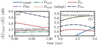
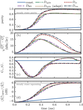
Figure 3 compares the dynamics of the time-continuous protocol of Ref. Kronwald et al. (2013) (blue solid lines) to those induced by optimized drives, using several target functionals and a total time of $1\text{\,}\mathrm{ms}$. The joint state purity and resonator squeezing are analyzed in Fig. 3(a) and (d), respectively. Moreover, Fig. 3(b) shows the difference $(G_{-}^{2}(t)-G_{+}^{2}(t))^{1/2}$, which determines an effective cooling rate into the squeezed state while Fig. 3(c) shows the ratio $G_{+}(t)/G_{-}(t)$, an effective rate determining the squeezing strength of the final steady state, cf. Ref. Kronwald et al. (2013). Pulses optimized using $D_{\mathrm{HS}}$ or $D_{\mathrm{split}}$ result in an acceleration of the thermalization process, cf. the blue solid vs. purple double-dashed, brown dotted and green dashed-double dotted lines in Fig. 3(a). These lines all converge to the proper joint state purity. Similarly, the resonator squeezing reaches the desired value for the corresponding curves in Fig. 3(d) and does so significantly faster for all optimized pulses.

Inspection of Fig. 3(b) and (c) allows us to unravel the control strategy. It consists, independently of the target functional, in an increase of the effective cooling rate $(G_{-}^{2}(t)-G_{+}^{2}(t))^{1/2}$ in order to speed up the cooling into the (squeezed) steady state. In general, ramping up $G_{-}$ and $G_{+}$ will always accelerate the coherent part of the dynamics, since the norm of the Hamiltonian (21) determines the timescale of the system’s coherent dynamics. However, ramping up the coupling also changes the steady state of the driven dissipative dynamics. Thus, the increase of $(G_{-}^{2}(t)-G_{+}^{2}(t))^{1/2}$, which is in our case in fact achieved by increasing both $G_{-}(t)$ and $G_{+}(t)$, needs to be balanced by a modulation of $G_{+}(t)/G_{-}(t)$ to ensure steering the system towards the correct target state. Interestingly, the optimizations with both $D_{\mathrm{HS}}$ (purple double-dashed lines) and $D_{\mathrm{split}}$ (green dashed-double dotted and brown dotted lines) find almost identical control fields. This is not guaranteed due to non-uniqueness of the control solution in most cases and indicates that we explore comparable optimization landscapes Moore Tibbetts et al. (2013); Riviello et al. (2015) despite the different functionals.

Note that the optimized control fields of Fig. 3(b-c) only require a slow modulation of the drive amplitudes while keeping their frequencies constant. This makes them experimentally feasible with existing technology—such slow modulations can easily be realized by arbitrary waveform generators allowing for amplitude modulations on timescales down to sub-nanoseconds Rogers et al. (2011) or even significantly more complex pulse shapes, see e.g. Ref. Häberle et al. (2013) for one example.

Another concern that often arises in the context of experimental feasibility of optimal control protocols is robustness with respect to noise in the controls. We therefore examine whether our optimized drives are robust with respect to amplitude noise. To this end, we apply $0.2\%,0.5\%$ and $1.0\%$ constant noise to the optimized field shapes  by rescaling the field amplitudes accordingly. We obtain for the final trace distance $D_{\mathrm{tr}}$ with respect to the targeted squeezed steady state an average of $3.7\cdot 10^{-4}$, $9.2\cdot 10^{-4}$ and $1.8\cdot 10^{-3}$, respectively. This needs to be compared to $D_{\mathrm{tr}}=4.8\cdot 10^{−6}$ for the original optimized fields and to $D_{\mathrm{tr}}=2.6\cdot 10^{−2}$ which one would obtain under the evolution with constant drives up to that point in time. The increase of the absolute error, of the order of $10^{-4}-10^{-3}$, is not surprising giving the order of the noise which is $10^{-3}-10^{-2}$.

Figure 4(a) provides a closer look at the asymptotic squeezing dynamics of Fig. 3(d), showing that only pulses optimized with $D_{\mathrm{HS}}$ and $D_{\mathrm{split}}$ reach the correct squeezing at final time, cf. the purple double-dashed and brown dotted lines. In contrast, the fields optimized with $D_{\mathrm{re}}$ and $D_{\mathrm{sm}}$ (red dashed and dark blue dot-dashed lines in Fig. 3) fail to steer the system towards a state with the correct purity. Instead, they act in order to increase the purity at final time $T$ as much as possible, failing to reach, however, completely pure states which are not attainable due to the finite temperature ($n_{\mathrm{th}}>0$). Figures 3 and 4(a) thus illustrate once more that the target functionals $D_{\mathrm{re}}$ and $D_{\mathrm{sm}}$ should not be used for non-pure target states.

Interestingly, the dynamics shown in Fig. 4(a) all results in a comparable squeezing with the final values $\langle\mathsf{\hat{X}}_{1}^{2}\rangle_{\mathrm{ZPF}}/\langle\mathsf{\hat{X}}_{1}^{2}\rangle$ obtained with $D_{\mathrm{re}}$ and $D_{\mathrm{sm}}$ even beyond the intended steady state squeezing of roughly 5.7 dB, cf. the red dashed and dark blue dot-dashed lines in Fig. 4(a). This indicates a larger squeezing to be possible than the one set by the steady state with its corresponding tradeoff between squeezing strength and purity. The apparently “good” optimization results with respect to the final-state squeezing obtained with $D_{\mathrm{re}}$ and $D_{\mathrm{sm}}$ in Fig. 4(a) can be explained by the fact that squeezing of any state is mainly determined by its direction on the generalized Bloch sphere. Here, the optimization benefits from the fact that $D_{\mathrm{re}}$ and $D_{\mathrm{sm}}$ try to match the final state directions. However, this is not always the case, as illustrated in Fig. 4(b) showing the squeezing dynamics for a similar optimization as in Fig. 3 but with a final time of $5\text{\,}\mathrm{ms}$. Note that for the constant protocol of Ref. Kronwald et al. (2013) the optimal relation $G_{+}/G_{-}$ of driving strengths which maximizes the squeezing strength can be estimated by $n_{\mathrm{th}}$ and the cooperativity $\mathcal{C}$. However, this estimation is no longer easily possible for shaped driving fields since they give rise to time-dependent cooperativities $\mathcal{C}(t)$.

Figure 5: Dynamics of the trace distance $D_{\mathrm{tr}}$, cf. Eq. (11), under the guess and optimized fields of Fig. 3. Beyond $T=$1\text{\,}\mathrm{ms}$$ (indicated by vertical line) all optimized fields are extended by the constant fields of the original, time-independent protocol.

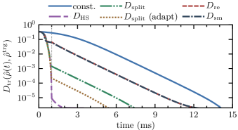
If the state preparation errors obtained with the optimized fields after $1\text{\,}\mathrm{ms}$ are not yet sufficient, it should be possible to continue approaching the steady state using the original protocol Kronwald et al. (2013) of constant drives. This is examined in Fig. 5 which shows the evolution of the trace distance $D_{\mathrm{tr}}$, cf. Eq. (11), under constant drives and optimized fields from Fig. 3(b) and (c), switched back to constant drives at $T=$1\text{\,}\mathrm{ms}$$. $D_{\mathrm{tr}}$ continues to decrease for times larger than the switching time, i.e., the final time used in the optimization. A monotonous decrease of $D_{\mathrm{tr}}$ across the switching time, as observed in Fig. 5, is expected for the fields optimized with $D_{\mathrm{split}}$ and $D_{\mathrm{HS}}$. It does not need to be the case, however, for the fields optimized with $D_{\mathrm{re}}$ or $D_{\mathrm{sm}}$. Here, the state at the switching time, although already closer to the target state than with constant driving, is still comparatively far from the steady state. Nevertheless, upon subsequent propagation with constant drives, $D_{\mathrm{tr}}$ is further improved in all cases. Figure 5 thus provides another illustration of the speed up in preparing the squeezed steady state.

Figure 6: (a) Peak and average cooperativity $\mathcal{C}$, calculated from the optimized fields $G_{-}(t)$, required to achieve a state preparation error of at most $D_{\mathrm{tr}}<10^{-4}$, as function of the total optimization time $T$ (employing $D_{\mathrm{HS}}$ for all optimizations). The horizontal line indicates the static cooperativity used in the experiment reported in Ref. Wollman et al. (2015). (b) Minimal time against required cooperativity to reach a steady state with $D_{\mathrm{tr}}<10^{-4}$ for the original, time-constant protocol of Ref. Kronwald et al. (2013). Note that each point in (b) corresponds to a different steady state while all points in (a) correspond to the same steady state.

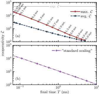
Finally, Fig. 6 answers the question by how much the approach of the steady state can be accelerated. The price for speed-up is cooperativity, or, in other words, laser intensity, as illustrated by Fig. 6(a). It shows the peak and average cooperativity $\mathcal{C}$, determined by the optimized field $G_{-}(t)$, as a function of the total optimization time $T$. Given an experimental bound on the cooperativity $\mathcal{C}$, one can thus easily determine the required time $T$ to reach the target state. Taking the experimental value of the cooperativity reported in Ref. Wollman et al. (2015), we find a speedup of at least two orders of magnitude, see Fig. 6(a), compared to the original protocol employing constant drives Kronwald et al. (2013). Conversely, fixing a certain duration $T$ determines the required cooperativity or laser power. Durations as short as $T=$0.07\text{\,}\mathrm{ms}$$ are feasible, while the state preparation errors are still sufficiently small with $D_{\mathrm{tr}}<10^{-4}$ for all points in Fig. 6(a). Moreover, the optimized pulse shapes corresponding to the data from Fig. 6(a) all look quite similar to the ones presented in Fig. 3(b) and (c).

Both peak and average cooperativity of the optimized field increase with decreasing duration, as one would expect for reaching the same target in less time. We observe an almost perfect power law dependence of the cooperativity $\mathcal{C}$ as a function of the duration $T$ in Fig. 6(a). This power law should be compared to the intrinsic scaling of the system due to its non-linearity which is shown in Fig. 6(b). Note that each point in Fig. 6(b) corresponds to a different steady state while all points in Fig. 6(a) correspond to the same steady state, namely the one used as benchmark in Fig. 3 after $15\text{\,}\mathrm{ms}$. The similar scaling observed in Fig. 6(a) and (b) thus indicates the system non-linearity to be the defining feature even in the case of time-dependent and optimized drives.

Note that the short fields with cooperativities $\mathcal{C}\sim 10^{4}$ approach the regime where the rotating wave approximation starts to break down Kronwald et al. (2013). Hence, we chose not to examine shorter, respectively stronger fields in Fig. 6.

III.3 Performance of optimization functionals

Figure 7: Convergence behavior of optimization algorithm for the target functionals used in Fig. 3. The weighting of the two terms in $D_{\mathrm{split}}$ was chosen as $\alpha_{1}=\alpha_{2}=1/2$, cf. Eq. (17), for the green dashed double-dotted line, while it was adapted after each iteration for the brown dotted line (see text).

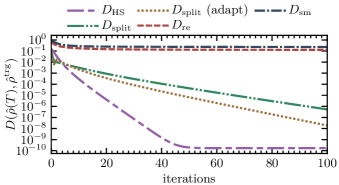
The convergence behavior of the optimization algorithm for the various target functionals used in Fig. 3 is inspected in Fig. 7. The functional value of $D_{\mathrm{re}}$ and $D_{\mathrm{sm}}$ rapidly approaches a plateau which indicates that the optimization got stuck and no improvement with respect to the guess pulses could be realized. In contrast, optimizations with $D_{\mathrm{HS}}$ (purple double-dashed line) and $D_{\mathrm{split}}$ (green dashed-double dotted and brown dotted lines) show an improvement of several orders of magnitude. For the optimizations with $D_{\mathrm{split}}$, we have used two different variants. For the green dashed double-dotted line constant, equivalent weights $\alpha_{1},\alpha_{2}$, cf. Eq. (17), have been used, while for the brown dotted line we have employed an automated update scheme for the weights after each iteration. In the latter case, we have adjusted the weights for the next iteration $i+1$,

$$\alpha_{1}^{(i+1)}=\frac{D_{\mathrm{angle}}^{(i)}}{D_{\mathrm{angle}}^{(i)}+D_{\mathrm{radius}}^{(i)}}\,,\quad\alpha_{2}^{(i+1)}=\frac{D_{\mathrm{radius}}^{(i)}}{D_{\mathrm{angle}}^{(i)}+D_{\mathrm{radius}}^{(i)}}\,,$$ (24)

using values of the current iteration $i$. This effectively causes the dominating term to become preferentially minimized within the next iteration. Although breaking strict monotonic convergence of Krotov’s method over multiple iterations, due to optimizing a different functional in each iteration, it yields better convergence in our example. The plateau of $D_{\mathrm{HS}}$ at $\sim 10^{-10}$, starting at iteration $\sim 50$, is not of physical origin but caused by the propagation accuracy; choosing a finer time discretization would probably allow the optimization to reach even smaller values.

Note that the scaling parameters $\lambda_{k}$, cf. Eq. (2), have been individually chosen for the different functionals in all optimizations shown in Fig. 7 . The necessity of different scalings is readily explained by the co-states $\mathsf{\hat{\chi}}_{l}(T)$, since their norm influences the magnitude of the field updates, via Eq. (5b). Due to different norms for different functionals, the optimization parameters $\lambda_{k}$ must usually be adjusted when switching functionals if one wants to maintain field updates of similar magnitude.

Figure 8: Comparison between changes in various distance measures under optimization with $D_{\mathrm{HS}}$ and $D_{\mathrm{split}}$, cf. Fig. 3.

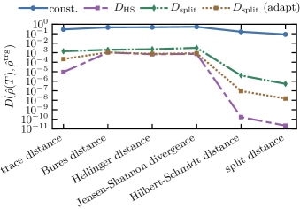
In the same context, one might naively conjecture from Fig. 7 that, because $D_{\mathrm{HS}}$ yields smaller functional values than $D_{\mathrm{split}}$, $D_{\mathrm{HS}}$ yields better optimization results. However, such a statement would in general be wrong. As discussed above in Sec. II.3, the accuracy with which the target state is reached is not uniquely assessed by a single measure. A small value of $D_{\mathrm{HS}}$ does not necessarily imply a similarly good value for any other distance measure. Figure 8 therefore displays the value of several reliable distance measures for the final state obtained with the fields optimized using $D_{\mathrm{HS}}$ and $D_{\mathrm{split}}$ and compares it with the non-optimized protocol, i.e., constant driving (blue line). We indeed observe that the optimization with $D_{\mathrm{HS}}$ (purple double-dashed line) yields the smallest state-preparation errors also for all other distance measures in Fig. 8.

This does not need to hold in general, however, since the absolute value of any distance measure $D$ is not to be confused with relative physical closeness of two states. While the measures $D$ considered in Fig. 8 are all known to be reliable, they assess state mismatches differently for $D>0$. For instance, if $D(\mathsf{\hat{\rho}}_{2},\mathsf{\hat{\rho}}^{\mathrm{trg}})>D(\mathsf{\hat{\rho}}_{1},\mathsf{\hat{\rho}}^{\mathrm{trg}})>0$ for two states $\mathsf{\hat{\rho}}_{1},\mathsf{\hat{\rho}}_{2}$, a desired target state $\mathsf{\hat{\rho}}^{\mathrm{trg}}$, and a measure $D$ does not imply the same to be true for another measure $\tilde{D}$. In other words, two reliable measures can still disagree on which of two states is closer to the target even though they both correctly assess when a state becomes identical to the target.

For the presented problem, the performance of the Hilbert-Schmdidt distance $D_{\mathrm{HS}}$ compared to the split-functional $D_{\mathrm{split}}$ is slightly better, cf. Fig. 7 and 8. Nevertheless, $D_{\mathrm{split}}$ contains information about angle and length mismatch of the Bloch vectors individually and thus provides more insight into the dominating source of mismatch which $D_{\mathrm{HS}}$ cannot provide. While this information was not of relevance here it could certainly be of interest for other optimization problems.

IV Conclusions

We have studied how to speed up evolution towards a squeezed steady state in a driven optomechanical system, consisting of cavity and mechanical resonator coupled via radiation pressure. To this end, we have replaced the constant drives of the original protocol Kronwald et al. (2013) by time-dependent pulses and derived the corresponding pulse shapes using quantum optimal control theory. To the best of our knowledge, our work is the first to apply quantum optimal control to cavity optomechanics. Further potential of quantum optimal control for this popular experimental platform is highlighted by a recent proposal suggesting to couple the cavity additionally to a two-level system in order to drive the mechanical oscillator into a Fock state Bergholm et al. (2018).

Our control solutions for accelerating the approach of a squeezed steady state consist in increasing the effective optomechanical coupling at intermediate times. At final time, the value of the constant coupling is resumed, ensuring approach of the proper steady state. We find the cooperativity corresponding to the increased optomechanical coupling due to the optimized fields to grow polynomially with decreasing protocol duration, for both average and peak value. Limiting the maximum cooperativity to that of the experiment reported in Ref. Wollman et al. (2015), a speed up of more than two orders of magnitude is possible, compared to the protocol using constant drives. The required pulse shapes correspond to simple modulations and are feasible with current technology using e.g. arbitrary wave form generators. In view of using the squeezed state, for example in quantum sensing, such a speed up will be important to minimize the detrimental influence of decoherence.

Since the steady state balances quantum mechanical purity and resonator squeezing, the control problem targets a non-pure state, and care must be taken when defining the target functional. In particular, functionals based on state overlaps fail when both states—the true state and the target state—are mixed. A possible remedy consists in replacing the overlap by a (modified) distance measure Xu et al. (2004). We have visualized the failure of overlap based functionals by examining the state vectors on the Bloch sphere: While the overlap only seeks to match the angle, a reliable figure of merit needs to match both angle and length of the vectors. This geometric picture provides the intuition for defining an alternative target functional, based on matching angle and length of the Bloch vectors separately. We have successfully employed this target functional as an alternative to a functional based on the Hilbert Schmidt distance Xu et al. (2004), obtaining fairly similar solutions to the control problem at hand. Moreover, we observe that optimization with both functionals not only leads to a minimization of the respective distance measure that is being employed but also to a reduction of any other distance measure that can be used to assess the state preparation error.

Our results of accelerated state preparation are relevant when exploiting squeezed states, for example in quantum sensing. Moreover, our Bloch vector based target functional should be useful, in general, to estimate quantum speed limits Campaioli et al. (2018). While the mismatch in Bloch vector angles quantifies rotation (i.e., unitary) errors, that in Bloch vector length estimates dissipative errors. If, for a given system, one can find an expression for the evolution speed of Bloch vector angle and length, this would allow to determine separate quantum speed limits for the unitary and dissipative parts of a system’s evolution. One could thus decide which of the two sets the overall speed limit.

Our results also give rise to an interesting further question in the context of squeezed state preparation. Incidentally, we have found fields that, while not resulting in the correct steady state, produce larger squeezing than expected for the steady state, with higher purity. This suggests to directly maximize the squeezing at final time, irrespective of the state at that time, instead of targeting a specific squeezed state as we have done here. Such an optimization is possible by taking the expectation value of the relevant quadrature as target functional. It would allow to examine the conditions for avoiding the trade-off between purity and squeezing to which the steady state is subject to Kronwald et al. (2013) and, more generally, determine the ultimate limit of quantum mechanical squeezing.