A Library for Constraint Consistent Learning

Abstract

This paper introduces the first, open source software library for Constraint Consistent Learning (CCL). It implements a family of data-driven methods that are capable of (i) learning state-independent and -dependent constraints, (ii) decomposing the behaviour of redundant systems into task- and null-space parts, and (iii) uncovering the underlying null space control policy . It is a tool to analyse and decompose many everyday tasks, such as wiping, reaching and drawing. The library also includes several tutorials that demonstrate its use with both simulated and real world data in a systematic way. This paper documents the implementation of the library, tutorials and associated helper methods. The software is made freely available to the community, to enable code reuse and allow users to gain in-depth experience in statistical learning in this area.

1 Introduction

Constraint Consistent Learning (Constraint Consistent LearningCCLConstraint Consistent Learning) is a family of methods for learning different parts of the equations of motion of redundant and constrained systems in a data-driven fashion Howard2009b ; Towell2010 ; Lin2015 . It is able to learn representations of self-imposed or environmental constraints Lin2015 ; LinHumanoid ; Armesto2017 , decompose the movement of redundant systems into task- and null space parts LinTaskConstraint ; Towell2010 , and uncover the underlying null space control policy Howard2009 ; Howard2008a . Constraint Consistent Learning enables:

1. Learning the constraints encountered in many everyday tasks through various representations.

2. Learning the underlying control behaviour from movements observed under different constraints.

In contrast to many standard learning approaches that incorporate the whole of the observed motions into a single control policy estimate schaal2003computational , Constraint Consistent Learning separates the problem into learning (i) the constraint representations and (ii) the underlying control policy . This provides more flexibility to the robot in the reproduction of the behaviour, for example, in face of demonstration data of one behaviour recorded under different constraints, Constraint Consistent Learning can learn a single policy that generalises across the constraints Howard2008a .

In terms of 1), the type of constraints may fall into the categories of state independent or state dependent constraints. For example, for state-space represented as end-effector coordinates, when wiping a table (see Figure 1(b)), the flat surface acts as a hard restriction on the actions available (motions perpendicular to the surface will be eliminated by the constraint), regardless of where the effector is located on the surface, so represents a state independent constraint. When wiping or stirring soup in a bowl (see Figure 1(c)), the curved surface introduces a state dependency in the constraint, since the restriction of motion is dependent on the location of the effector. The ability to predict how the constraints can influence the outcomes of control actions can speed-up learning of the new skills and enhance safety (e.g., the learned constraints can prevent exploration actions that cause excessive force). Furthermore, the availability of constraint knowledge can reduce the dimension of the search space when optimising behaviours Bitzer2010 .

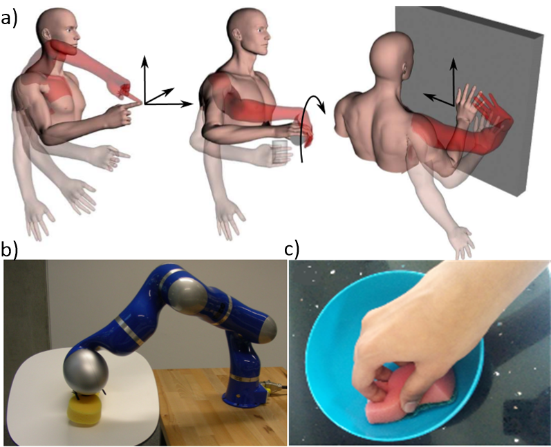
Figure 1: Typical examples in CCL. (a) Three different tasks: moving the finger to an $x,y,z$, position, liquid pouring and wiping a surface. In each case, redundancy is resolved in the same way. (b) A table wiping task is subject to a state-independent flat environment constraint using a robot arm. (c) A bowl wiping task subject to a state-dependent curvature constraint.

In terms of 2), the observable movements may contain partial information about the control policy masked by the constraint, or higher priory task objectives Towell2010 . For example, in a reaching task (see Figure 1(a)), humans move their arms towards the target (primary task) while minimising effort, for instance, by keeping the elbow low (secondary objective). The imperative of executing the primary task represents a self-imposed constraint, that restricts the secondary objective. Interaction with environmental constraints, can also mask the actions applied by the demonstrator. For example, when grasping an object on a table such as a pen, the fingers slide along the table surface resulting in a discrepancy between the observed motion and that predicted by the applied actions were the surface different in shape or orientation. Constraint Consistent Learning can help uncover these components, enabling the intended actions to be reconstructed and applied to new situations LinEtAl2018 .

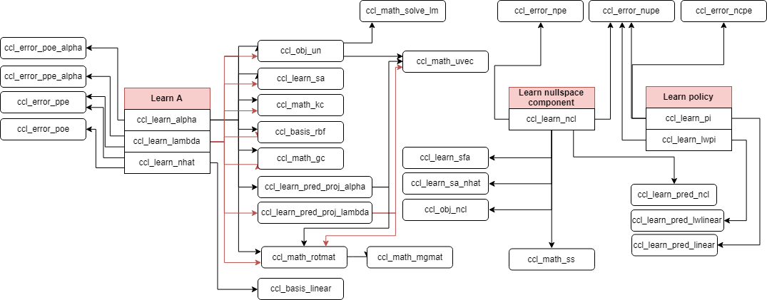
Figure 2: A system diagram of the Constraint Consistent Learning library. The complete dependency tree can be found in the package documentation. The library has been written under three categories: learn A, learn null-space component and learn policy. The arrows links the dependencies of the implementations to the main functions.

This paper introduces the Constraint Consistent Learning library as a community resource for learning in the face of kinematic constraints, alongside tutorials to guide users who are not familiar with learning constraint representations and underlying policies. As its key feature, Constraint Consistent Learning is capable of decomposing many everyday tasks (e.g., wiping Lin2015 , reaching Towell2010 and gait Lin2014a ) and learn subcomponents (e.g., null space components Towell2010 , constraints Lin2015 and unconstrained control policy Howard2008a ) individually. The methods implemented in the library provide means by which these quantities can be extracted from the data, based on a collection of algorithms developed since Constraint Consistent Learning was first conceived in 2007 Howard2007 . It presents the first unified Application Programmers Interface (Application Programmers InterfaceAPIApplication Programmers Interface) implementing and enabling use of these algorithms in a common framework.

2 Application Domain

The Constraint Consistent Learning library addresses the problem of learning from motion subject to various constraints for redundant systems. The behaviour of constrained and redundant systems is well-understood from an analytical perspective Udwadia1996 , and a number of closely related approaches have been developed for managing redundancy at the levels of dynamics Peters2008a , kinematics Liegeois1977 ; Whitney1969 , and actuation Howard2011 ; Tahara2009 . However, a common factor in these approaches is the assumption of prior knowledge of the constraints, the control policies, or both. Constraint Consistent Learning addresses the case where there are uncertainties in these quantities and provides methods for their estimation.

2.1 Constraint Formalism

The Constraint Consistent Learning library assumes training data to come from systems subject to the following formalism.

The system is considered to be subject to a set of $\mathcal{{S}}$-dimensional ($\mathcal{{S}}\leq\mathcal{{Q}}$) constraints with the general form

$$\mathbf{A}(\mathbf{x})\mathbf{u}(\mathbf{x})=\mathbf{b}(\mathbf{x})$$ (1)

where $\mathbf{x}\in\mathbb{R}^{\mathcal{{P}}}$ represents state and $\mathbf{u}\in\mathbb{R}^{\mathcal{{Q}}}$ represents the action. $\mathbf{A}(\mathbf{x})\in\mathbb{R}^{\mathcal{{S}}\times\mathcal{{Q}}}$ is the constraint matrix which projects the task space policy onto the relevant part of the control space. The vector term $\mathbf{b}\in\mathbb{R}^{\mathcal{{S}}}$, if present, represents constraint-imposed motion (in redundant systems, it is the policy in task space).

Inverting (1), results in the relation

$$\mathbf{u}(\mathbf{x})=\underbrace{{\mathbf{A}(\mathbf{x})}^{\dagger}\mathbf{b}(\mathbf{x})}_{\mathbf{v}}+\underbrace{\mathbf{N}(\mathbf{x})\boldsymbol{\pi}(\mathbf{x})}_{\mathbf{w}}$$ (2)

where ${\mathbf{A}}^{\dagger}$ denotes the unique Moore-Penrose pseudo-inverse of the matrix $\mathbf{A}$, $\mathbf{N}(\mathbf{x})=(\mathbf{I}-{\mathbf{A}(\mathbf{x})}^{\dagger}\mathbf{A}(\mathbf{x}))\in\mathbb{R}^{\mathcal{{Q}}\times\mathcal{{Q}}}$ is a projection matrix that projects the policy $\boldsymbol{\pi}(\mathbf{x})$ onto the null space of the constraint. Note that, the constraint can be state dependent ($\mathbf{A}(\mathbf{x})$) or state independent ($\mathbf{A}$). $\mathbf{v}(\mathbf{x})\equiv{\mathbf{A}(\mathbf{x})}^{\dagger}\mathbf{b}(\mathbf{x})$ and $\mathbf{w}(\mathbf{x})\equiv\mathbf{N}(\mathbf{x})\boldsymbol{\pi}(\mathbf{x})$ are termed the task-space and the null-space component, respectively. Typically, it is assumed that the only directly observable quantities are the state-action pairs $(\mathbf{x}_{n},\mathbf{u}_{n})$ $n\in 1,\cdots,\mathcal{{N}}$ which contain an unknown combination of $\mathbf{v}(\mathbf{x})$ and $\mathbf{w}(\mathbf{x})$, or at greater granularity $\mathbf{A}(\mathbf{x})$, $\mathbf{b}(\mathbf{x})$, $\mathbf{N}(\mathbf{x})$ and $\boldsymbol{\pi}(\mathbf{x})$. The Constraint Consistent Learning library provides methods for estimating each of these quantities—implementation details are provided in §3.

Note that, application of learning approaches klanke2008library that do not consider the composition of the data in terms of the constraints are prone to poor performance and modelling errors. For example, applying direct regression to learn policies where there are variations in the constraints can result in model averaging effects that risk unstable behaviour Howard2009b . This is due to factors such as (i) the non-convexity of observations under different constraints, and (ii) degeneracyin the set of possible policies that could have produced the movement under the constraint . Providing an open-source collection of software tools suitable for application to this class of learning problems, can help those working in the field to avoid these pitfalls.

3 Implementation

A system diagram of the Constraint Consistent Learning library is shown in Figure 2. The naming convention is following ccl_xxx_xxx indicating the category and functionality of the implementations. The following provides brief notes on the implementation languages and library installation, explains the data structures used in toolbox.

3.1 Language and Installation Notes

The library is implemented in both C and Matlab and is available for download from Github . The Constraint Consistent Learning library is provided under the GNU General Public License v3.0, and documentation is provided online. To use the Matlab package, the user can just add the Constraint Consistent Learning library into the current path. Installation of the C package has been tested on Ubuntu 14.04 Linux systems and is made easy through use of the autoconf utility. For Windows systems, only the Matlab package is currently tested and supported. The C package’s only dependency is on the 3rd-party, open-source GNU Scientific Library (GNU Scientific LibraryGSLGNU Scientific Library).

A detailed explanation of the functions follows, alongside tutorial examples that are provided to enable the user to easily extend use of the library to their chosen application (see §6).

3.2 Data Structures

The methods implemented in the toolbox work on data that is given as tuples $\{\mathbf{x}_{n},\mathbf{u}_{n}\}_{n=1}^{\mathcal{{N}}}$ of observed states and constrained actions. It is assumed that all the actions $\mathbf{u}$ are generated using the same underlying policy $\boldsymbol{\pi}(\mathbf{x})$. In particular $\mathbf{u}_{n}={\mathbf{A}_{n}}^{\dagger}\mathbf{b}_{n}+\mathbf{N}_{n}\boldsymbol{\pi}_{n}$, where $\mathbf{A}_{n}$, $\mathbf{b}_{n}$ and $\boldsymbol{\pi}_{n}$ are not explicitly known. The observations are assumed to be grouped into $\mathcal{K}$ subsets of $\mathcal{{N}}$ data points, each (potentially) recorded under different (task or environmental) constraints.

The Constraint Consistent Learning library uniformly stores the data tuples in a data structure reflecting this problem structure. The latter includes the data fields incorporating samples of the input state ($\mathbf{x}$), action ($\mathbf{u}$), actions from unconstrained policy ($\boldsymbol{\pi}$), task space component ($\mathbf{v}$) and null space component ($\mathbf{w}$). The major data structure and data fields are listed in Table 1.

Table 1: Main data structures of the Constraint Consistent Learning library. dim* indicates the data fields for definition of the data dimensionality.

Struct	Main Fields	Definition	Other Fields
data	X	$\mathbf{X}=(\mathbf{x}_{1},\cdots,\mathbf{x}_{\mathcal{{N}}})\in\mathbb{R}^{\mathcal{{P}}\times\mathcal{{N}}}$
	U	${\mathbf{U}}=(\mathbf{u}_{1},\cdots,\mathbf{u}_{\mathcal{{N}}})\in\mathbb{R}^{\mathcal{{Q}}\times\mathcal{{N}}}$
	Pi	$\mathbf{\Pi}=(\boldsymbol{\pi}_{1},\cdots,\boldsymbol{\pi}_{\mathcal{{N}}})\in\mathbb{R}^{\mathcal{{Q}}\times\mathcal{{N}}}$
	Ts	${\mathbf{V}}=(\mathbf{v}_{1},\cdots,\mathbf{v}_{\mathcal{{N}}})\in\mathbb{R}^{\mathcal{{Q}}\times\mathcal{{N}}}$
	Un	${\mathbf{W}}=(\mathbf{w}_{1},\cdots,\mathbf{w}_{\mathcal{{N}}})\in\mathbb{R}^{\mathcal{{Q}}\times\mathcal{{N}}}$
model	M	Nullspace component Model weighting parameters $\mathbf{\omega}$.
	c	$\mathbf{\mu}$
	s	$\mathbf{\Sigma}$
	phi	$\boldsymbol{\beta}$
			dim*
search	theta	$(\boldsymbol{\theta}_{1},\cdots,\boldsymbol{\theta}_{\mathcal{{N_{S}}}})$
			dim*
optimal	nmse	Normalised mean square error.
	f_proj	Function handle for projection matrix.
			dim*
options	TolFun	Tolerance for residual.
	TolX	Tolerance for model parameters.
	MaxIter	Maximum iterations for optimiser.
			dim*
stats	nmse	Normalised mean square error.
	mse	Mean squared error.
	var	Variance.

Learning is more effective when the data contains sufficiently rich variations in one or more of the quantities defined in (2), since methods learn the consistency by teasing out the variations. For instance, when learning $\mathbf{v}$, variations in $\mathbf{w}$ are desirable Towell2010 . For learning $\boldsymbol{\pi}$, observations subject to multiple constraints (variation in $\mathbf{A}$) are necessary Howard2009b . For learning constraint $\mathbf{A}$, variations in $\boldsymbol{\pi}$ are desirable LinTaskConstraint .

4 Learning Functions

The Application Programmers Interface of the Constraint Consistent Learning library provides functions for a series of algorithms for the estimation of the quantities $\mathbf{A}$, $\mathbf{v}$, $\mathbf{w}$ and $\boldsymbol{\pi}$. The following provides a summary of the methods provided, including implementation notes and a brief summary of the theoretical basis for each algorithm.

4.1 Learning the Constraint Matrix

The library implements several methods for estimating the constraint matrix $\mathbf{A}$. These assume that (i) each observation contains a constraint $\mathbf{A}\neq\boldsymbol{0}$, (ii) the observed actions take the form $\mathbf{u}=\mathbf{w}=\mathbf{N}\boldsymbol{\pi}$, (iii) $\mathbf{u}$are generated using the same null space policy $\boldsymbol{\pi}$, and (iv) $\mathbf{A}$is not explicitly known for any observation (optionally, features in form of candidate rows of $\mathbf{A}$, may be provided as prior knowledge–see §4.1.2).

The methods for learning $\mathbf{A}$ under these assumptions, are based the insight that the projection of $\mathbf{w}$ also lies in the same image space Lin2015 , i.e.,

$$(\mathbf{I}-{\mathbf{A}}^{\dagger}\mathbf{A})\mathbf{w}=\mathbf{N}\mathbf{w}=\mathbf{w}.$$ (3)

If the estimated constraint matrix $\tilde{\mathbf{A}}$ is accurate, it should also obey this equality. Hence, the estimate can be formed by minimising the difference between the left and right hand sides of (3), as captured by the error function

$$E[\tilde{\mathbf{N}}]=\sum^{\mathcal{{N}}}_{n=1}||\mathbf{w}_{n}-\tilde{\mathbf{N}}_{n}\mathbf{w}_{n}||^{2}$$ (4)

where $\tilde{\mathbf{N}}_{n}=\mathbf{I}-{\tilde{\mathbf{A}}_{n}}^{\dagger}\tilde{\mathbf{A}}_{n}$. This can be expressed in simplified form

$$E[\tilde{\mathbf{A}}]=\sum^{\mathcal{{N}}}_{n=1}||\mathbf{w}_{n}^{\top}{\tilde{\mathbf{A}}_{n}}^{\dagger}\tilde{\mathbf{A}}_{n}\mathbf{w}_{n}||^{2}.$$ (5)

Note that, in forming the estimate, no prior knowledge of $\boldsymbol{\pi}$ is required. However, an appropriate representation of the constraint matrix is needed. As outlined in §1, in the context of learning $\mathbf{A}$, there are two distinct cases depending on whether the constraints are state-dependent or not. The Constraint Consistent Learning library implements methods for both scenarios.

4.1.1 Learning State Independent Constraints

The simplest situation occurs if the constraint is unvarying throughout the state space. In this case, the constraint matrix can be represented as the concatenation of a set of unit vectors

$$\tilde{\mathbf{A}}=(\hat{\mathbf{a}}_{1}^{\top},\hat{\mathbf{a}}_{2}^{\top},\cdots,\hat{\mathbf{a}}_{\mathcal{{S}}}^{\top})^{\top}$$ (6)

where the $s$th unit vector $\hat{\mathbf{a}}_{s}$ is constructed from the parameter vector $\boldsymbol{\theta}\in\mathbb{R}^{\mathcal{{Q}}-1}$ that represents the orientation of the constraint in action space (see Lin2015 for details).

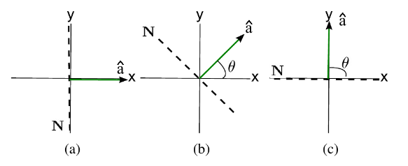
Figure 3: Three one-dimensional unit vector constraints $\hat{\mathbf{a}}$ where (a) $\theta=0^{\circ}$, (b) $\theta=45^{\circ}$, and (c) $\theta=90^{\circ}$ (reproduced from Lin2015 ).

A visualisation of the simplest case of a one-dimensional constraint in a system with two degrees of freedom where $\mathbf{A}=\hat{\mathbf{a}}\in\mathbb{R}^{1\times 2}$ is shown in Figure 3. It can be seen how $\boldsymbol{\theta}$ (in this case, $\hat{\mathbf{a}}=(\cos{\theta},\sin{\theta})$) corresponds to different estimates of the constraint its associated null-space.

The Constraint Consistent Learning library provides the function optimal =ccl_learna_nhat(Un )

to form the estimate $\tilde{\mathbf{A}}$ in this scenario, where Un is the collated set of samples of $\mathbf{w}$ (see Table 1) and optimal is the learnt model. The C counterpart of this function is ⬇ void learn_nhat (const double *Un,const int dim_u, const int dim_n,NHAT_Model *optimal) where the input argument Un and output argument optimal in the C library is identical with Matlab implementation. The arguments dim_u and dim_n are used for defining the dimensionality of the array Un.

The function works by searching for rows of the estimated constraint matrix $\tilde{\mathbf{A}}$ using the function ⬇ [model, stats] = ccl_learna_sfa (UnUn,Un,model,search)

the arguments model and search contain the initial model (untrained) model, parameters controlling the search, respectively and UnUn is the matrix ${\mathbf{W}}^{\top}{\mathbf{W}}$ where ${\mathbf{W}}$ is a matrix containing samples of $\mathbf{w}$. This is pre-calculated prior to the function call for speed. The function returns the learnt model model and learning statistics stats (see Table 1).

4.1.2 Learning State Dependent Constraint

Another proposed method for learning a state-dependent constraint, i.e., the constraint $\mathbf{A}(\mathbf{x})$ depends on the current state of the robot $\mathbf{x}$. For learning $\mathbf{A}(\mathbf{x})$, two scenarios may be encountered where (i) there is prior knowledge of the constraint in form of candidate rows (see LinTaskConstraint ), or (ii) no prior knowledge is available .

In the case of (i),

$$\mathbf{A}(\mathbf{x})=\tilde{\boldsymbol{\Lambda}}(\mathbf{x})\boldsymbol{\Phi}(\mathbf{x}).$$ (7)

$\boldsymbol{\Phi}(\mathbf{x})\in\mathbb{R}^{R\times\mathcal{{Q}}}$ is the feature matrix and $\tilde{\boldsymbol{\Lambda}}(\mathbf{x})\in\mathbb{R}^{\mathcal{{S}}\times R}$ is the selection matrix specifying which rows represent constraints. The feature matrix can take the form $\boldsymbol{\Phi}(\mathbf{x})=\mathbf{J}(\mathbf{x})$, where $\mathbf{J}$ is the Jacobian mapping from the joint space to the end-effector task space. Similar to (6), $\tilde{\boldsymbol{\Lambda}}(\mathbf{x})$ is described by a set of $\mathcal{{S}}$ orthonormal vectors

$$\tilde{\boldsymbol{\Lambda}}(\mathbf{x})=(\boldsymbol{\lambda}_{1}(\boldsymbol{\theta})^{\top},\boldsymbol{\lambda}_{2}(\boldsymbol{\theta})^{\top},\cdots,\boldsymbol{\lambda}_{\mathcal{{S}}}(\boldsymbol{\theta})^{\top})^{\top}$$ (8)

where $\boldsymbol{\lambda}_{s}\in\mathbb{R}^{\mathcal{{S}}}$ is the $s$th dimension in the task space and $\boldsymbol{\lambda}_{i}\perp\boldsymbol{\lambda}_{j}$ for $i\neq j$. Parameter $\boldsymbol{\theta}_{s}\in\mathbb{R}^{\mathcal{{S}}-1}$ is used for representing the constraint vector $\boldsymbol{\lambda}$. Each $\boldsymbol{\theta}_{s}$ is modelled as $\boldsymbol{\theta}_{s}=\mathbf{\omega}_{s}\boldsymbol{\beta}(\mathbf{x})$ where $\mathbf{\omega}_{s}\in\mathbb{R}^{(\mathcal{{Q}}-1)\times G}$ is the weight matrix, and $\boldsymbol{\beta}(\mathbf{x})\in\mathbb{R}^{G}$ is the vector of $G$ basis functions that transform $\mathbf{x}$ into a set of feature vectors in higher dimensional space. Substituting $\tilde{\mathbf{A}}_{n}=\tilde{\boldsymbol{\Lambda}}_{n}\boldsymbol{\Phi}_{n}$, (5) can be written as

$$E[\tilde{\boldsymbol{\Lambda}}]=\sum^{\mathcal{{N}}}_{n=1}||\mathbf{u}_{n}^{\top}{(\tilde{\boldsymbol{\Lambda}}_{n}\boldsymbol{\Phi}_{n})}^{\dagger}\tilde{\boldsymbol{\Lambda}}_{n}\boldsymbol{\Phi}_{n}\mathbf{u}_{n}||^{2}.$$ (9)

The optimal $\tilde{\boldsymbol{\Lambda}}$ can be formed by iteratively searching the choice of $\boldsymbol{\lambda}_{s}$ that minimises (9).

The objective function for (5) and ((9)) are embedded in function

⬇

[fun] = ccl_obj_AVn (model,W,BX,RnUnUnn)

where fun is the objective function handle, M is the model parameter $\mathbf{\omega}$, BX is the feature vectors in high dimension space $\boldsymbol{\beta}(\mathbf{x})$, and RnUnUnn is the pre-rotated $UnUn_{n}$.

The implementation of case (i) is:

⬇

[optimal] =

ccl_learn_lambda (Un,X,Phi,options)

Where Phi is the feature matrix $\boldsymbol{\Phi}$. The implementation of case (ii) where

$$\mathbf{A}(\mathbf{x})=(\mathbf{a}_{1}(\boldsymbol{\theta})^{\top},\mathbf{a}_{2}(\boldsymbol{\theta})^{\top},\cdots,\mathbf{a}_{\mathcal{{S}}}(\boldsymbol{\theta})^{\top})^{\top}$$ (10)

is:

⬇

[optimal] =

ccl_learn_alpha (Un,X,options)

The non-linear parameter optimisation solver used for learning $\boldsymbol{\theta}_{s}$ calculates the direction in which the parameter is improved for this, the Levenberg-Marquardt (LM) solver is used. The latter is embedded in the function

⬇

[xf,S,msg] = ccl_math_solve_lm (varargin)

where the inputs varargin are the objective function (fun), initial guess of model parameters (xc, i.e., $\mathbf{\omega}$) and training options (options).

4.2 Learning the Task and Null Space Components

When the unconstrained control policy is subject to both constraint and some task space policy ($\mathbf{b}(\mathbf{x})\neq\boldsymbol{0}$), it is often useful to extract the task and null space components ($\mathbf{v}(\mathbf{x})$ and $\mathbf{w}(\mathbf{x})$, respectively) of the observed actions $\mathbf{u}(\mathbf{x})$. The Constraint Consistent Learning library provides the following methods to estimate these quantities. These assume that the underlying null-space policy and the task constraint are consistent.

Assuming that the underlying null-space policy $\boldsymbol{\pi}(\mathbf{x})$ and the task constraint $\mathbf{A}(\mathbf{x})$ are consistent across the data set, the null space component $\mathbf{w}(\mathbf{x})$ should satisfy the condition $\mathbf{N}(\mathbf{x})\mathbf{u}(\mathbf{x})=\mathbf{w}(\mathbf{x})$ as noted in Towell2010 , in this case, $\mathbf{w}(\mathbf{x})$ by minimising

$$E[\tilde{\mathbf{w}}]=\sum^{\mathcal{{N}}}_{n=1}||\tilde{\mathbf{P}}_{n}\mathbf{u}_{n}-\tilde{\mathbf{w}}(\mathbf{x}_{n})||^{2}$$ (11)

with $\tilde{\mathbf{P}}_{n}=\tilde{\mathbf{w}}_{n}\tilde{\mathbf{w}}_{n}^{\top}/||\tilde{\mathbf{w}}_{n}||^{2}$, where $\tilde{\mathbf{w}}_{n}=\tilde{\mathbf{w}}(\mathbf{x}_{n})$ projects an arbitrary vector onto the same space of $\mathbf{w}$, and $\mathbf{u}_{n}$ is the $n$th data point. This error function eliminates the task-space components $\mathbf{v}(\mathbf{x})$ by penalising models that are inconsistent with the constraints, i.e., those where the difference between the model, $\tilde{\mathbf{w}}(\mathbf{x})$, and the observations projected onto that model is large (for details, see Towell2010 ). In the Constraint Consistent Learning library, this functionality is implemented in the function

⬇

[fun,J] = ccl_obj_ncl (model,W,BX,U)

where U is the observed actions ${\mathbf{U}}$. The outputs are fun (function handle) and J (analytical Jacobian of the objective function (11)).

Minimisation of (11) penalises models that are inconsistent with the constraints, i.e., those where the difference between the model, $\tilde{\mathbf{w}}_{k}(\mathbf{x})$, and the observations projected onto that model is large (for details, see Towell2010 ). In the Constraint Consistent Learning library, this functionality is implemented in the function

⬇

model = ccl_learnv_ncl(X,U,model)

where the inputs are X (input state), Y (observed actions combined with task and null space components) and model (model parameters). The output is the learnt model model.

4.3 Learning the Unconstrained Control Policy

The Constraint Consistent Learning library also implements methods for estimating the underlying unconstrained control policy ($\boldsymbol{\pi}(\mathbf{x})$). These assume either (i) $\mathbf{b}=0$ no additional task is involved or (ii) $\mathbf{w}$ is learnt using the method proposed in §4.2.

As shown in Howard2008a , an estimate $\tilde{\boldsymbol{\pi}}(\mathbf{x})$ can be obtained by minimising the inconsistency error

$$E_{\pi}=\sum^{\mathcal{{N}}}_{n=1}||\mathbf{u}_{n}-\mathbf{P}_{n}\tilde{\boldsymbol{\pi}}(\mathbf{x}_{n})||^{2};\quad\mathbf{P}_{n}=\frac{\mathbf{u}_{n}\mathbf{u}_{n}^{\top}}{||\mathbf{u}_{n}||^{2}}.$$ (12)

The risk function (12) is compatible with many regression models. The Constraint Consistent Learning library implements a parametric policy learning scheme. Where $\tilde{\boldsymbol{\pi}}(\mathbf{x})={\mathbf{W}}\boldsymbol{\beta}(\mathbf{x})$, ${\mathbf{W}}\in\mathbb{R}^{\mathcal{{Q}}\times M}$ is a matrix of weights and $\boldsymbol{\beta}(\mathbf{x})\in\mathbb{R}^{M}$ is a vector of fixed basis functions (e.g., linear features or Gaussian radial basis functions). A locally-weighted linear policy learning is also implemented in the library to improve the robustness of the policy learning (Details see Towell2010 ). A reinforcement learning scheme (with possibly deep network structure) can also be used to learn more complex policies Howard2013 ; Howard2013b ; Gu2016 .

The Constraint Consistent Learning library implements the learning of these models through the functions

⬇

model = ccl_learnp_pi (X,U,model)

where inputs X and U are observed states and actions. The outputs are the learnt model model.

5 Evaluation Criteria

For testing different aspects of the learning performance, a number of evaluation criteria have been defined in the Constraint Consistent Learning literature. These include metrics comparing estimation against the ground truth (if known), as well as those that provide a pragmatic estimate of performance based only on observable quantities. In the context of evaluating the constraints, the Constraint Consistent Learning library provides implementations of the following functions.

If the ground truth constraint matrix $\mathbf{A}_{n}$ and unconstrained policy $\boldsymbol{\pi}_{n}$ are known, then the normalised projected policy error (Normalised Constrained Policy Error) provides the best estimate of learning performance Lin2015 . In the Constraint Consistent Learning library, The Normalised Constrained Policy Error is computed through the functions

⬇

[nPPE,vPPE,uPPE] =

ccl_error_ppe (U_t,N_p,Pi)

where U_t is the true null space components ${\mathbf{W}}$, N_p is the learned projection matrix $\mathbf{N}$, and Pi is the unconstrained control policy $\boldsymbol{\pi}$. The outputs are the Normalised Constrained Policy Error, variance and (non-normalised) mean-squared PPE, respectively.

In the absence of ground truth $\mathbf{A}_{n}$ and $\boldsymbol{\pi}_{n}$, the normalised projected observation error (Normalised Constrained Policy Error) must to be used Lin2015 . The functions implemented for computing the Normalised Constrained Policy Error are

⬇

[nPOE,vPOE,uPOE] =

ccl_error_poe (U_t,N_p,Pi)

where the inputs and outputs conventions are similar to those of the functions computing the Normalised Constrained Policy Error.

To evaluate the predictions of the null-space component model $\tilde{\mathbf{w}}_{k}(\mathbf{x})$, the null space projection error (NPE) can be used Towell2010 . This is implemented in the function

⬇

[umse,v,nmse] = ccl_error_npe (Un,Unp)

where Un and Unp are the true and predicted null space component. The return values are the NPE, variance and (non-normalised) mean squared projection error. Note that, use of this function assumes knowledge of the ground truth $\mathbf{w}_{n}$.

Table 2: Key Functions in the CCL Library

Function Type	Name	Description
Learn Constraint	Learn Alpha	Learning state dependent projection N (9) + (8)
	Learn Lambda	Learning state dependent selection matrix $\tilde{\boldsymbol{\Lambda}}$ (9) + (10)
	Learn Nhat	Learning state independent constraint N (5)
Learn Nullspace Component	Learn ncl	Learn the nullspace component of u = v+w (11)
Learn unconstrained control Policy	Learn CCL Pi	Learn null space policy (12)
Evaluate Constraint error	NPPE	normalised projected policy error
	NPOE	normalised projected observation error
Evaluate Nullspace component error	NPE	nullspace projection error
Evaluate unconstrained control policy	NUPE	normalised unconstrained policy error
	NCPE	normalised constrained policy error

To evaluate the estimated unconstrained control policy model $\tilde{\boldsymbol{\pi}}(\mathbf{x})$, the normalised unconstrained policy error (NUPE) and normalised constrained policy error (NCPE) Howard2008a are used. The former assumes access to the ground truth unconstrained policy $\boldsymbol{\pi}_{n}$, while the latter assumes the true $\mathbf{w}_{n}$ is known. They are implemented in the functions

⬇

[umse,v,nmse] = ccl_error_nupe (F,Fp)

and

⬇

[umse,v,nmse] = ccl_error_ncpe(F,Fp,P)

where input F is the true unconstrained control policy commands, Fp is the learned unconstrained control policy and P is the projection matrix. The outputs are Normalised Unconstrained Policy Error (respectively, NCPE), the sample variance, and the mean squared Unconstrained Policy Error (respectively, Constrained Policy Error).

Table 2 shows an overview of all key functions as well as their respective equations for learning and evaluation which are covered in this section.

6 Tutorials

The Constraint Consistent Learning library package provides a number of tutorial scripts to illustrate its use. Multiple examples are provided which demonstrate learning using both simulated and real world data, including, learning in a simulated 2-link arm reaching task, and learning a wiping task. The following describes the toy example in detail, alongside a brief description of other included demonstrations which were tested with real world systems. Further details of the latter are included in the documentation.

In the first, a simple, illustrative toy example is used, in which a two-dimensional system is subject to a one-dimensional constraint. In this, the learning of (i) the null space components, (ii) the constraints, and (iii) the null space policy is demonstrated.

The toy example code has been split into three main sections for learning different parts of the equations. Detailed comments of the functions can be found in the Matlab script. The procedure for generating data is dependant on the part of the equation you wish to learn. Details can be found in the documentations.

6.0.1 Learning Null Space Components $\mathbf{w}$

This section gives a guidance of how to use the library for learning ${\mathbf{W}}$. A sample Matlab snippet is shown in Table 3 and explained as follows. Firstly, the user needs to generate training data given the assumption that $\mathbf{w}$ is fixed but $\mathbf{v}$ is varying in your demonstration. The unconstrained policy is a limit cycle policy LinHumanoid . For learning, the centre of the Radial Basis Function s are chosen according to K-means and the variance as the mean distance between the centres. A parametric model with 16 Gaussian basis functions is used. Then the null-space component model can be learnt through ccl_learnv_ncl. Finally, the evaluation metrics NUPE and NPE are used to report the learning performance.

6.0.2 Learning Null Space Constraints $\mathbf{A}$

This section gives guidance of how to use the library to learn a state independent $\mathbf{A}$ and state dependent $\mathbf{A}(\mathbf{x})$, where $\mathbf{b}=0$. A sample Matlab script is provided in Table 4 and explained as following. Firstly, it simulates a problem where the user faces is learning a fixed constraint in which the systems null-space controller $\boldsymbol{\pi}$ varies. For learning a linear constraint problem, constant $\mathbf{A}$ is used and ccl_learn_nhat is implemented. For learning a parabolic constraint, a state-dependent constraint $\mathbf{A}(\mathbf{x})$ of the form $\mathbf{A}(\mathbf{x})=[-2ax,1]$ is used. For this, ccl_learn_alpha is implemented. Finally, nPPE and nPOE are used to evaluate the learning performance.

Table 3: Sample code snippet for learning null-space component from Matlab

Data = ccl_data_gen(settings) ;

model.c = ccl_math_gc (X, model.dim_basis) ;

model.s = mean(mean(sqrt(ccl_math_distances(model.c, model.c))))^2 ;

model.phi = @(x)ccl_basis_rbf ( x, model.c, model.s);

model = ccl_learnv_ncl (X, U, model) ;

f_ncl = @(x) ccl_learnv_pred_ncl ( model, x ) ;

NSp = f_ncl (X) ;

NUPE = ccl_error_nupe(Un, Unp) ;

NPE = ccl_error_npe (Un, Unp) ;

Table 4: To do: Sample code snippet for learning state independent and dependent constraint from matlab

Data = ccl_data_gen(settings) ;

model = ccl_learn_nhat (Un) ; % for learning $\mathbf{A}$

model = ccl_learn_alpha (Un, X, settings) ; % for learning $\mathbf{A}(\mathbf{x})$

nPPE = ccl_error_ppe(U, model.P, Pi) ;

nPOE = ccl_error_poe(U, model.P, Pi) ;

Table 5: Sample code snippet for learning null-space control policy from Matlab

Data = ccl_data_gen(settings);

model.c = ccl_math_gc (X, model.dim_basis) ;

model.s = mean(mean(sqrt(ccl_math_distances(model.c, model.c))))^2 ;

model.phi = @(x)ccl_basis_rbf ( x, model.c, model.s);

model = ccl_learnp_pi (X, Un, model) ;

fp = @(x) ccl_learnp_pred_linear ( model, x ) ;

Pi = fp (X) ;

NUPE = ccl_error_nupe(Un, Unp) ;

NCPE = ccl_error_ncpe (Un, Unp) ;

6.0.3 Learning Null Space Policy $\pi$

This section will give guidance on learning an unconstrained control policy $\boldsymbol{\pi}$. This applies to the use case where $\boldsymbol{\pi}$ is consistent but $\mathbf{A}$ is varying. A sample Matlab script is provided in Table 5 and explained as the following. For learning, 10 Radial Basis Function s are used and learned using the same K-means algorithm. ccl_learnp_pi is then implemented for training the model. Finally, NUPE and NCPE are calculated to evaluate the model’s performance. In the library, a locally weighted policy learning method is also implemented in both Matlab and C. For details please refer to the documentation.

Other examples such as a 2-link arm and wiping examples are also implemented which follow a similar procedure to the toy example but in a higher dimension to aid novice users wanting to take advantage of the Constraint Consistent Learning to learn the kinematic redundancy of a robot. Moreover, users can easily adapt these learning methods, where the provided demonstrations such as wiping and real data are setup to use the 7 degrees of freedomKUKA LWR3 and Trakstar 3D electromagnetic tracking sensor, respectively, are reconfigured to suit their own systems and requirements.

7 Conclusion

This paper introduces the Constraint Consistent Learning library, an open-source collection of software tools for learning different components of constrained movements and behaviours. The implementations of the key functions have been explained throughout the paper, and interchangeable and expandable examples have been demonstrated using both simulated and real world data for their usage. For the first time, the library brings together a diverse collection of algorithms developed over the past ten years into a unified framework with a common interface for software developers in the robotics community. In the future work, Matlab and python wrappers will be released by taking advantage of the fast computation routine implemented in C.

References

- (1) M. Howard, S. Klanke, M. Gienger, C. Goerick, and S. Vijayakumar, “A novel method for learning policies from variable constraint data,” Auton. Robots, vol. 27, pp. 105–121, 2009.
- (2) C. Towell, M. Howard, and S. Vijayakumar, “Learning null space policies,” in IEEE. C. Intel. & Rob. Sys., 2010.
- (3) H.-C. Lin, M. Howard, and S. Vijayakumar, “Learning null space projections,” in ICRA, 2015.
- (4) V. Ortenzi, H. C. Lin, M. Azad, R. Stolkin, J. A. Kuo, and M. Mistry, “Kinematics-based estimation of contact constraints using only proprioception,” in Humanoids, Nov 2016, pp. 1304–1311.
- (5) L. Armesto, J. Moura, V. Ivan, A. Sala, and S. Vijayakumar, “Learning Constrained Generalizable Policies by Demonstration,” in Robotics: Sci. & Sys., 2017.
- (6) H.-C. Lin, P. Ray, and M. Howard, “Learning task constraints in operational space formulation,” in ICRA, 1 2017.
- (7) M. Howard, S. Klanke, M. Gienger, C. Goerick, and S. Vijayakumar, “A novel method for learning policies from constrained motion,” in ICRA, 2009.
- (8) M. Howard, S. Klanke, M. Gienger, C. Goerick, and S. Vijayakumar, “Behaviour generation in humanoids by learning potential-based policies from constrained motion,” Applied Bionics and Biomechanics, vol. 5, no. 4, pp. 195–211, Dec. 2008.
- (9) S. Schaal, A. Ijspeert, and A. Billard, “Computational approaches to motor learning by imitation,” Philos. Trans. R. Soc. Lond., B, Biol. Sci., vol. 358, no. 1431, pp. 537–547, 2003.
- (10) S. Bitzer, M. Howard, and S. Vijayakumar, “Using dimensionality reduction to exploit constraints in reinforcement learning,” in IEEE. C. Intel. & Rob. Sys., 2010.
- (11) H.-C. Lin, S. Rathod, and M.H., “Learning state dependent constraints,” 2018.
- (12) H.-C. Lin, M. Howard, and S. Vijayakumar, “A novel approach for representing and generalising periodic gaits,” Robotica, vol. 32, pp. 1225–1244, 12 2014.
- (13) M.H. and S. Vijayakumar, “Reconstructing null-space policies subject to dynamic task constraints in redundant manipulators,” in W. Rob. & Math., September 2007.
- (14) F. E. Udwadia and R. E. Kalaba, Analytical Dynamics: A New Approach. Cambridge University Press, 1996.
- (15) J. Peters, M. Mistry, F. E. Udwadia, J. Nakanishi, and S. Schaal, “A unifying framework for robot control with redundant DOFs,” vol. 24, pp. 1–12, 2008.
- (16) A. Liégeois, “Automatic supervisory control of the configuration and behavior of multibody mechanisms,” IEEE T. Sys., Man & Cyb., vol. 7, pp. 868–871, 1977.
- (17) D. E. Whitney, “Resolved motion rate control of manipulators and human prostheses,” vol. 10, no. 22, pp. 47–53, 1969.
- (18) M.H., D. Braun, and S. Vijayakumar, “Constraint-based equilibrium and stiffness control of variable stiffness actuators,” in ICRA, May 2011, pp. 5554–5560.
- (19) K. Tahara, S. Arimoto, M. Sekimoto, and Z.-W. Luo, “On control of reaching movements for musculo-skeletal redundant arm model,” Appl. Bionics & Biomech., vol. 6, pp. 11–26, 2009.
- (20) S. Klanke, S. Vijayakumar, and S. Schaal, “A library for locally weighted projection regression,” Journal of Machine Learning Research, vol. 9, no. Apr, pp. 623–626, 2008.
- (21) M. Howard and Y. Nakamura, “Locally weighted least squares temporal difference learning,” in European Symposium Artificial Neural Networks, 2013.
- (22) M. Howard and Y. Nakamura, “Locally weighted least squares policy iteration for model-free learning in uncertain environments,” in IEEE. C. Intel. & Rob. Sys., 2013.
- (23) S. Gu, E. Holly, T. Lillicrap, and S. Levine, “Deep Reinforcement Learning for Robotic Manipulation,” 2016.