AFLOW-QHA3P: Robust and automated method
to compute thermodynamic properties of solids

Abstract

Accelerating the calculations of finite-temperature thermodynamic properties is a major challenge for rational materials design. Reliable methods can be quite expensive, limiting their effective applicability in autonomous high-throughput workflows. Here, the 3-phonons quasi-harmonic approximation (QHA) method is introduced, requiring only three phonon calculations to obtain a thorough characterization of the material. Leveraging a Taylor expansion of the phonon frequencies around the equilibrium volume, the method efficiently resolves the volumetric thermal expansion coefficient, specific heat at constant pressure, the enthalpy, and bulk modulus. Results from the standard QHA and experiments corroborate the procedure, and additional comparisons are made with the recently developed self-consistent QHA. The three approaches — 3-phonons, standard, and self-consistent QHAs — are all included within the automated, open-source framework AFLOW, allowing automated determination of properties with various implementations within the same framework.

Introduction

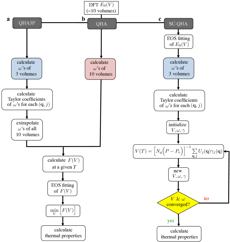
Figure 1: The workflows for (a) QHA3P compared with (b) QHA and (c) SC-QHA. The most time-consuming step of QHA is highlighted in red, while the time-saving steps of the other two methods are highlighted in blue.

Reliable and efficient computational methods are needed to guide time-consuming and laborious experimental searches, thus accelerating materials design. Implementing effective methods within automated frameworks such as AFLOW curtarolo:art65 ; curtarolo:art75 ; curtarolo:art92 ; curtarolo:art127 ; curtarolo:art128 facilitates the calculation of thermodynamic properties for large materials databases. There are several computational techniques to characterize the temperature dependent properties of materials, each with varying accuracy and computational cost. Techniques such as ab initio molecular dynamics Yu_SR_2016 ; Kresse_PRB_1993 ; Sarnthein_PRB_1996 ; Zhang_APL_2015 ; Jesson_APL_2015 and the stochastic self-consistent harmonic approximation Errea_PRL_2013 ; Errea_PRB_2014 give accurate results for the temperature dependent properties of materials. Although these methods are highly accurate, the treatment of anharmonicity requires the consideration of many large distorted structural configurations, making them computationally prohibitive for screening large materials sets. Other methods including the Debye-Grüneisen model BlancoGIBBS2004 ; Poirier_Earth_Interior_2000 or Machine Learning approaches curtarolo:art124 ; curtarolo:art136 require less computational resources, but often struggle to predict properties such as the Grüneisen parameter with reasonable accuracy curtarolo:art96 ; curtarolo:art115 . The quasi-harmonic approximation (QHA) Liu_Cambridge_2016 ; Wang_ACTAMAT_2004 ; Duong_jap_2011 balances accuracy and computational cost for calculating temperature and pressure dependent properties of materials.

In its standard formulation, QHA also remains too expensive for automated screening curtarolo:art114 . QHA requires many independent phonon spectra calculations, obtained by diagonalizing the dynamical matrices giving eigenvectors (modes) and eigenvalues (energies) Ziman_Oxford_1960 ; ThermoCrys ; Dove_LatDynam_1993 ; PhysPhon . The dynamical matrix can be constructed either with “linear response” PhysPhon ; BaroniRMP2001 or the “finite displacements” method PhysPhon ; Axel_RMP ; curtarolo:art125 . Despite its low computational demands, linear response does not perform well at high temperatures where anharmonicity can be large. The finite displacements method can be easily integrated with a routine that computes forces, making the preferred method for high-throughput calculations. However, it is still computationally expensive for (i) low symmetry crystals, (ii) materials with large atomic variations leading to complicated optical branches, and (iii) metallic systems having long-range force interactions requiring large supercells. In order to make QHA more suitable for automated screening, it is necessary to reduce the number of required phonon spectra.

Recently, the self-consistent quasi-harmonic approximation Huang_cms_2016 (SC-QHA) has been developed. It self-consistently minimizes the external and internal pressures. The method requires spectra at only two or three volumes, while the frequency-volume relationship is determined using a Taylor expansion. It is computationally efficient and almost five times faster than QHA. Results agree well with experiments at low temperatures, although some deviations are observed at high-temperature for the tested systems Huang_cms_2016 .

In this article, the quasi-harmonic approximation 3-phonons (QHA3P) method is introduced. It calculates the phonon frequencies around equilibrium for only three different volumes, and performs a Taylor expansion to extrapolate the phonon frequencies at other volumes. The QHA3P approach drastically reduces the computational cost and achieves consistency with experiments, allowing automated materials’ property screening without compromising accuracy. Similar to QHA, QHA3P minimizes the Helmholtz free energy with respect to volume for each temperature. The calculation of the thermodynamic properties, and the temperature dependent electronic contribution to the free energy, are the same as in QHA, enabling unrestricted screening of all types of materials. The QHA, SC-QHA, and QHA3P methods are all implemented within AFLOW curtarolo:art114 ; curtarolo:art65 ; curtarolo:art75 ; curtarolo:art92 ; curtarolo:art127 ; curtarolo:art128 . The performance of QHA3P with two different exchange-correlation (XC) functionals is investigated.

Computational details

The thermal properties of materials at finite temperatures are calculated from the Helmholtz free energy $\left(F\right)$, which depends on temperature $\left(T\right)$ and volume $\left(V\right)$. Neglecting the electron-phonon coupling and magnetic contributions, $F$ can be written as the sum of three additive contributions Liu_Cambridge_2016 ; Wang_ACTAMAT_2004 ; Duong_jap_2011 :

$$F\left(V,T\right)=E_{\begin{subarray}{c}\scalebox{0.6}{0}\end{subarray}}\left(V\right)+F_{\begin{subarray}{c}\scalebox{0.6}{vib}\end{subarray}}\left(V,T\right)+F_{\begin{subarray}{c}\scalebox{0.6}{elec}\end{subarray}}\left(V,T\right),$$ (1)

where $E_{\begin{subarray}{c}\scalebox{0.6}{0}\end{subarray}}$ is the total energy of the system at $0$ K without any atomic vibrations, $F_{\begin{subarray}{c}\scalebox{0.6}{vib}\end{subarray}}$ is the vibrational free energy of the lattice ions, and $F_{\begin{subarray}{c}\scalebox{0.6}{elec}\end{subarray}}$ is the finite temperature electronic free energy due to thermal electronic excitations.

QHA Methodology. QHA enables the calculation of $F_{\begin{subarray}{c}\scalebox{0.6}{vib}\end{subarray}}$ via the harmonic approximation and includes anharmonic effects in the form of volume dependent phonon frequencies. $F_{\begin{subarray}{c}\scalebox{0.6}{vib}\end{subarray}}$ is given by curtarolo:art114 ; Duong_jap_2011 ; Wang_ACTAMAT_2004 ; Liu_Cambridge_2016 :

$$F_{\begin{subarray}{c}\scalebox{0.6}{vib}\end{subarray}}\left(V,T\right)=\frac{1}{N_{q}}\sum_{{\bf q},j}\left(\frac{\hbar\omega_{j}({\bf q})}{2}+k_{{\begin{subarray}{c}\scalebox{0.6}{B}\end{subarray}}}T{\rm ln}\left[1-{\mathrm{exp}}\left(-\frac{\hbar\omega_{j}(\bf q)}{k_{{\begin{subarray}{c}\scalebox{0.6}{B}\end{subarray}}}T}\right)\right]\right),$$ (2)

where $\hbar$ and $k_{\begin{subarray}{c}\scalebox{0.6}{B}\end{subarray}}$ are the Planck and Boltzmann constants, and $\omega_{j}(\bf q)$ is the volume dependent phonon frequency (at ${\bf q},j$). The (${\bf q},j$) comprises both the wave vector q and phonon branch index $j$. $N_{q}$ is the total number of wave vectors.

Although $F_{\begin{subarray}{c}\scalebox{0.6}{elec}\end{subarray}}\left(V,T\right)$ is negligible for wide band gap materials, its contribution is required for metals and narrow band-gap systems. $F_{\begin{subarray}{c}\scalebox{0.6}{elec}\end{subarray}}\left(V,T\right)$ is calculated as Wang_ACTAMAT_2004 ; Arroyave_ACTAMAT_2005 ; Liu_Cambridge_2016 :

$$\begin{split}F_{\begin{subarray}{c}\scalebox{0.6}{elec}\end{subarray}}\left(V,T\right)=&U_{\begin{subarray}{c}\scalebox{0.6}{elec}\end{subarray}}\left(V,T\right)-TS_{\begin{subarray}{c}\scalebox{0.6}{elec}\end{subarray}}\left(V,T\right),\\ U_{\begin{subarray}{c}\scalebox{0.6}{elec}\end{subarray}}\left(V,T\right)=&\int_{0}^{\infty}n_{\begin{subarray}{c}\scalebox{0.6}{elec}\end{subarray}}\left(\epsilon\right)f\left(\epsilon\right)\epsilon{\rm d}\epsilon-\int_{0}^{E_{\rm F}}n_{\begin{subarray}{c}\scalebox{0.6}{elec}\end{subarray}}\left(\epsilon\right)\epsilon{\rm d}\epsilon,\\ S_{\begin{subarray}{c}\scalebox{0.6}{elec}\end{subarray}}\left(V,T\right)=&-k_{{\begin{subarray}{c}\scalebox{0.6}{B}\end{subarray}}}\int_{0}^{\infty}n_{\begin{subarray}{c}\scalebox{0.6}{elec}\end{subarray}}\left(\epsilon\right)[f\left(\epsilon\right){\rm ln}\left(f\left(\epsilon\right)\right)+\\ &+\left(1-f\left(\epsilon\right)\right){\rm ln}\left(1-f\left(\epsilon\right)\right)]{\rm d}\epsilon,\end{split}$$ (3)

where $U_{\begin{subarray}{c}\scalebox{0.6}{elec}\end{subarray}}\left(V,T\right)$ and $S_{\begin{subarray}{c}\scalebox{0.6}{elec}\end{subarray}}\left(V,T\right)$ are the temperature dependent parts of the electronic internal energy and the electronic entropy respectively, $n_{\begin{subarray}{c}\scalebox{0.6}{elec}\end{subarray}}(\epsilon)$ is the density of states at energy $\epsilon$, $f(\epsilon)$ is the Fermi-Dirac distribution, and $E_{\rm F}$ is the Fermi energy.

The QHA method requires at least ${\sim}10$ $E_{\begin{subarray}{c}\scalebox{0.6}{0}\end{subarray}}$ and ${\sim}10$ phonon calculations $\left(F_{{\begin{subarray}{c}\scalebox{0.6}{vib}\end{subarray}}}\right)$ in order to obtain a good fit for the equation of state (EOS). QHA is generally implemented using isotropic volume distortions, although its implementation in AFLOW can also include anisotropic effects by considering $F$ as a function of direction-dependent strain, e.g. along principal directions Tohei_JAP_2016 ; Hermet_JPCC_2014 . The calculated $E_{\begin{subarray}{c}\scalebox{0.6}{0}\end{subarray}}$ and $F_{{\begin{subarray}{c}\scalebox{0.6}{vib}\end{subarray}}}$ are fitted to an EOS (e.g., Birch-Murnaghan EOS Fu_PRB_1983 ). The equilibrium volume $\left(V_{\begin{subarray}{c}\scalebox{0.6}{eq}\end{subarray}}\right)$ at a given temperature is determined by minimizing $F$ with respect to $V$ at a given $T$, $\left(\partial F/\partial V\right)_{\scalebox{0.6}{T}}{=}0$ (Figure 1b). A more detailed description of $F{-}V$ interpolation and the calculation of different energy terms is discussed in Ref. curtarolo:art114 .

The thermodynamic properties — constant volume specific heat $\left(C_{{\begin{subarray}{c}\scalebox{0.6}{V}\end{subarray}}}\right)$, constant pressure specific heat $\left(C_{{\begin{subarray}{c}\scalebox{0.6}{P}\end{subarray}}}\right)$, average Grüneisen parameter $\left({\bar{\gamma}}\right)$, and volumetric thermal expansion coefficient $\left(\alpha_{\begin{subarray}{c}\scalebox{0.6}{V}\end{subarray}}\right)$ curtarolo:art114 ; Duong_jap_2011 ; Wang_ACTAMAT_2004 ; Liu_Cambridge_2016 — are calculated according to the following definitions:

$$C_{{\begin{subarray}{c}\scalebox{0.6}{V}\end{subarray}}} = k_{{\begin{subarray}{c}\scalebox{0.6}{B}\end{subarray}}}\sum_{{\bf q},j}\left(\frac{\hbar\omega_{j}({\bf q},V_{\begin{subarray}{c}\scalebox{0.6}{0}\end{subarray}})}{k_{{{\begin{subarray}{c}\scalebox{0.6}{B}\end{subarray}}}}T}\right)^{2}\frac{{\mathrm{exp}}\left({\frac{\hbar\omega_{j}({\bf q},V_{\begin{subarray}{c}\scalebox{0.6}{0}\end{subarray}})}{k_{{{\begin{subarray}{c}\scalebox{0.6}{B}\end{subarray}}}}T}}\right)}{\left({\mathrm{exp}}{\left(\frac{\hbar\omega_{j}({\bf q},V_{\begin{subarray}{c}\scalebox{0.6}{0}\end{subarray}})}{k_{{{\begin{subarray}{c}\scalebox{0.6}{B}\end{subarray}}}}T}\right)}-1\right)^{2}}$$ (4)

$$C_{{\begin{subarray}{c}\scalebox{0.6}{P}\end{subarray}}} = C_{{\begin{subarray}{c}\scalebox{0.6}{V}\end{subarray}}}+V_{{\begin{subarray}{c}\scalebox{0.6}{eq}\end{subarray}}}TB\alpha_{\begin{subarray}{c}\scalebox{0.6}{V}\end{subarray}}^{2},$$ (5)

$${\bar{\gamma}} = \frac{\sum_{{\bf q},j}\gamma_{j}({\bf q})c_{j}({\bf q})}{\sum_{{\bf q},j}c_{j}({\bf q})},$$ (6)

$$\alpha_{\begin{subarray}{c}\scalebox{0.6}{V}\end{subarray}} = \frac{C_{{\begin{subarray}{c}\scalebox{0.6}{V}\end{subarray}}}{\bar{\gamma}}}{BV_{{\begin{subarray}{c}\scalebox{0.6}{eq}\end{subarray}}}},$$ (7)

where $\omega_{j}({\bf q},V_{\begin{subarray}{c}\scalebox{0.6}{0}\end{subarray}})$ is the frequency of phonon mode (${\bf q},j$) at relaxed volume ($V_{{\begin{subarray}{c}\scalebox{0.6}{0}\end{subarray}}}$), and $c_{j}(\bf q)$ and $\gamma_{j}(\bf q)$ are the specific heat capacity at constant volume and mode Grüneisen at (${\bf q},j$). The definitions of the bulk modulus ($B$) and mode Grüneisen parameter, ($\gamma_{j}(\bf q)$), are

$$B = V_{{{\begin{subarray}{c}\scalebox{0.6}{eq}\end{subarray}}}}\left(\frac{\partial^{2}F}{\partial V^{2}}\right)_{T},$$ (8)

$$\gamma_{j}(\bf q) = -\frac{V_{\begin{subarray}{c}\scalebox{0.6}{0}\end{subarray}}}{\omega_{j}({\bf q},V_{\begin{subarray}{c}\scalebox{0.6}{0}\end{subarray}})}\left(\frac{\partial\omega_{j}(\bf q)}{\partial V}\right)_{{\begin{subarray}{c}\scalebox{0.6}{V}\end{subarray}}_{{\begin{subarray}{c}\scalebox{0.6}{0}\end{subarray}}}},$$ (9)

For metals and small band gap materials, the electronic contribution can be considerable and is included in the thermodynamic definitions. After including the electronic contribution, $\alpha_{\begin{subarray}{c}\scalebox{0.6}{V}\end{subarray}}$ and $C_{{\begin{subarray}{c}\scalebox{0.6}{P}\end{subarray}}}$ are re-formulated as Hermet_JPCC_2014 ; Solyom_Springer_2007 :

$$\begin{split}\alpha_{{\begin{subarray}{c}\scalebox{0.6}{V}\end{subarray}},{{\begin{subarray}{c}\scalebox{0.6}{ph+elec}\end{subarray}}}}&=\alpha_{{\begin{subarray}{c}\scalebox{0.6}{V}\end{subarray}}}+\alpha_{{\begin{subarray}{c}\scalebox{0.6}{V}\end{subarray}},{{\begin{subarray}{c}\scalebox{0.6}{elec}\end{subarray}}}}=\frac{C_{{\begin{subarray}{c}\scalebox{0.6}{V}\end{subarray}}}{\bar{\gamma}}}{BV_{{{\begin{subarray}{c}\scalebox{0.6}{eq}\end{subarray}}}}}+\frac{2}{3BV_{{\begin{subarray}{c}\scalebox{0.6}{eq}\end{subarray}}}}C_{{{\begin{subarray}{c}\scalebox{0.6}{V}\end{subarray}}},{{\begin{subarray}{c}\scalebox{0.6}{elec}\end{subarray}}}},\\[5.0pt] C_{{{\begin{subarray}{c}\scalebox{0.6}{P}\end{subarray}}},{{\begin{subarray}{c}\scalebox{0.6}{ph+elec}\end{subarray}}}}&=C_{{\begin{subarray}{c}\scalebox{0.6}{V}\end{subarray}}}+V_{{\begin{subarray}{c}\scalebox{0.6}{eq}\end{subarray}}}TB\alpha_{{\begin{subarray}{c}\scalebox{0.6}{V}\end{subarray}}}^{2}+C_{{{\begin{subarray}{c}\scalebox{0.6}{V}\end{subarray}}},{{\begin{subarray}{c}\scalebox{0.6}{elec}\end{subarray}}}},\\[5.0pt] C_{{{\begin{subarray}{c}\scalebox{0.6}{V}\end{subarray}}},{{\begin{subarray}{c}\scalebox{0.6}{elec}\end{subarray}}}}&=T\left(\frac{\partial S_{{\begin{subarray}{c}\scalebox{0.6}{elec}\end{subarray}}}}{\partial T}\right)_{\begin{subarray}{c}\scalebox{0.6}{V}\end{subarray}}.\end{split}$$ (10)

In addition to the basic quasi-harmonic thermodynamic properties, the enthalpy $\left(H\right)$ of a structure at $P$=0 Duong_jap_2011 ; Arroyave_ACTAMAT_2005 is:

$$H=F\left(T\right)+TS=F\left(T\right)-T\frac{\partial{F\left(T\right)}}{\partial T}.$$ (11)

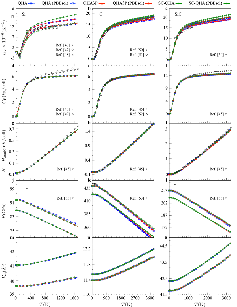
Figure 2: The thermodynamic properties of Si (a,d,g,j,m), C (b,e,h,k,n), and SiC (c,f,i,l,o) are presented up to their melting temperatures ($T_{\scalebox{0.6}{m}}$): $1687$, $3823$ and $3000$ K Barin_1993 , respectively. The results are obtained with QHA3P, QHA and SC-QHA using the PBE and PBEsol XC functionals. Experimental results from different sources Gibbons_PR_1958 ; Yim_JAP_1978 ; Okada_JAP_1984 ; Chase_AIP_1998 ; Barin_1993 ; Slack_JAP_1975 ; Skinner_AM_1957 ; Victor_JCP_1962 ; McSkimin_JAP_1972 ; Li_JAP_1986 ; Csonka_PRB_2009 are indicated by inverted triangles, diamonds, and pentagons.

AFLOW implementation of SC-QHA. SC-QHA has also been implemented within AFLOW following the description of Ref. Huang_cms_2016 . Similar to QHA, SC-QHA calculates $E_{\begin{subarray}{c}\scalebox{0.6}{0}\end{subarray}}$ at ${\sim}10$ different volumes, but requires only three phonon calculations at different cell volumes (Figure 1c) Huang_cms_2016 . It computes the temperature-dependent unit-cell volume by optimizing the total pressure (external, electronic, and phononic pressures),

$$V=\left[\left(P-P_{\begin{subarray}{c}\scalebox{0.6}{e}\end{subarray}}\right)\right]^{-1}\times\frac{1}{N_{q}}\sum_{{\bf q},j}U_{j}({\bf q})\gamma_{j}({\bf q}),$$ (12)

where $P$ is external pressure, $P_{\begin{subarray}{c}\scalebox{0.6}{e}\end{subarray}}\left(=-{\rm d}E_{\begin{subarray}{c}\scalebox{0.6}{0}\end{subarray}}\left(V\right)/{\rm d}V\right)$ is the electronic pressure, $U_{j}({\bf q})$ is the mode vibrational internal energy and $\gamma_{j}(\bf q)$ is the mode Grüneisen parameter at (${\bf q},j$). The volume dependent $\omega_{j}({\bf q})$ and $\gamma_{j}({\bf q})$ are extrapolated to other volumes using a Taylor expansion:

$$\begin{split}\omega_{j}\left({\bf q},V\right)&=\omega_{j}\left({\bf q},V_{\begin{subarray}{c}\scalebox{0.6}{0}\end{subarray}}\right)+\left(\frac{\partial\omega_{j}({\bf q})}{\partial V}\right)_{{\begin{subarray}{c}\scalebox{0.6}{V}\end{subarray}}_{{\begin{subarray}{c}\scalebox{0.6}{0}\end{subarray}}}}(\Delta V)\\ &+\frac{1}{2}\left(\frac{\partial^{2}\omega_{j}({\bf q})}{\partial V^{2}}\right)_{{\begin{subarray}{c}\scalebox{0.6}{V}\end{subarray}}_{{\begin{subarray}{c}\scalebox{0.6}{0}\end{subarray}}}}\left(\Delta V\right)^{2},\end{split}$$ (13)

$$\gamma_{j}\left({\bf q},V\right)=-\frac{V}{\omega_{j}({\bf q})}\left[\left(\frac{\partial\omega_{j}({\bf q})}{\partial V}\right)_{{\begin{subarray}{c}\scalebox{0.6}{V}\end{subarray}}_{{\begin{subarray}{c}\scalebox{0.6}{0}\end{subarray}}}}+\left(\frac{\partial^{2}\omega_{j}({\bf q})}{\partial V^{2}}\right)_{{\begin{subarray}{c}\scalebox{0.6}{V}\end{subarray}}_{{\begin{subarray}{c}\scalebox{0.6}{0}\end{subarray}}}}\Delta V\right],$$ (14)

where $\Delta V{=}V{-}V_{\begin{subarray}{c}\scalebox{0.6}{0}\end{subarray}}$. Computing the second order derivative of $\omega_{j}({\bf q})$ requires the calculation of phonon spectra at three different volumes. Due to its numerical accuracy, the central difference algorithm is used to calculate the derivative with respect to volume. $U_{j}({\bf q})$, the mode vibrational internal energy, is defined as

$$U_{j}({\bf q}) = \left[\left({{\mathrm{exp}}\left(\frac{\hbar\omega_{j}({\bf q})}{k_{{{\begin{subarray}{c}\scalebox{0.6}{B}\end{subarray}}}}T}\right)-1}\right)^{-1}+\frac{1}{2}\right]\hbar\omega_{j}({\bf q}).$$ (15)

The procedure to self-consistently optimize the volume at zero external pressure ($P{=}0$) and finite $T$ is as follows Huang_cms_2016 (Figure 1c):

1. First, ${\sim}10$ $E_{\begin{subarray}{c}\scalebox{0.6}{0}\end{subarray}}\left(V\right)$ values are fitted to the EOS, enabling the analytical calculation of $P_{\begin{subarray}{c}\scalebox{0.6}{e}\end{subarray}}$ at any new volume.

2. $\left(\partial\omega_{j}({\bf q})/\partial V\right)_{{\begin{subarray}{c}\scalebox{0.6}{V}\end{subarray}}_{{\begin{subarray}{c}\scalebox{0.6}{0}\end{subarray}}}}$ and $\left(\partial^{2}\omega_{j}({\bf q})/\partial V^{2}\right)_{{\begin{subarray}{c}\scalebox{0.6}{V}\end{subarray}}_{{\begin{subarray}{c}\scalebox{0.6}{0}\end{subarray}}}}$ are calculated from the three phonon spectra, where $\omega_{j}({\bf q})$ and $\gamma_{j}({\bf q})$ are initialized to their values at $V_{\begin{subarray}{c}\scalebox{0.6}{0}\end{subarray}}$.

3. To compute the equilibrium volume at $T$, $V$ is initialized to a value $0.2\%$ larger than $V_{\begin{subarray}{c}\scalebox{0.6}{0}\end{subarray}}$ and the following loop is iterated:

   1. Calculate $P_{\begin{subarray}{c}\scalebox{0.6}{e}\end{subarray}}$ using the EOS, and $\sum_{{\bf q},j}U_{j}({\bf q})\gamma_{j}({\bf q})$ using $\omega_{j}({\bf q})$ and $\gamma_{j}({\bf q})$.

   2. Update the value of $V$ using Eq. (12), and update $\omega_{j}({\bf q})$ and $\gamma_{j}({\bf q})$ using Eq. (13 - 14), respectively.

   3. If $V$ is not converged to within an acceptable threshold (e.g., $10^{-6}$), then loop over steps (i) and (ii).

   4. Calculate other thermodynamic properties using the converged values of $\omega_{j}({\bf q})$ and $\gamma_{j}({\bf q})$.

   5. $V$, $\omega_{j}({\bf q})$, and $\gamma_{j}({\bf q})$ values at a given $T$ are used as the initial values for the next $T$ characterization.

In SC-QHA, at low temperatures (e.g., $0.1$ K), $V_{\begin{subarray}{c}\scalebox{0.6}{eq}\end{subarray}}$ is calculated self-consistently. At higher temperatures, $V_{\begin{subarray}{c}\scalebox{0.6}{eq}\end{subarray}}$ is extrapolated as $V_{{\begin{subarray}{c}\scalebox{0.6}{eq}\end{subarray}}}\left(T+\Delta T\right)\simeq\left(1+\alpha_{\begin{subarray}{c}\scalebox{0.6}{V}\end{subarray}}\Delta T\right)V_{\begin{subarray}{c}\scalebox{0.6}{eq}\end{subarray}}$, as described in Ref. Huang_cms_2016 , in order to avoid self-consistent volume calculations for each $T$. $V_{\begin{subarray}{c}\scalebox{0.6}{eq}\end{subarray}}$ is equal to the self-consistently converged $V$ at a given $T$. Similarly, all of the properties calculated at $V_{\begin{subarray}{c}\scalebox{0.6}{eq}\end{subarray}}$ are the equilibrium properties at $T$.

While $C_{\begin{subarray}{c}\scalebox{0.6}{V}\end{subarray}}$, $C_{\begin{subarray}{c}\scalebox{0.6}{P}\end{subarray}}$, and $\alpha_{\begin{subarray}{c}\scalebox{0.6}{V}\end{subarray}}$ are the same as for QHA, $B$ and $\gamma_{j}({\bf q})$ are computed differently in SC-QHA. Here:

$$B = V_{{{\begin{subarray}{c}\scalebox{0.6}{eq}\end{subarray}}}}\left(\frac{{\rm d}^{2}E_{\begin{subarray}{c}\scalebox{0.6}{0}\end{subarray}}}{{\rm d}V^{2}}\right)_{V_{{{\begin{subarray}{c}\scalebox{0.6}{eq}\end{subarray}}}}}+B_{\gamma}+B_{\Delta\gamma}+P_{\gamma},$$ (16)

where $B_{\gamma}$ and $B_{\Delta\gamma}$ are the bulk modulus contributions due to phonons, while $P_{\gamma}$ represents the bulk modulus contribution due to external pressure. The mathematical expressions for these variables are defined in Ref. Huang_cms_2016 , and $\gamma_{j}({\bf q})$ is computed using Eq. (14). It is also important to note that the value of $C_{\begin{subarray}{c}\scalebox{0.6}{V}\end{subarray}}$ at given $T$ is computed with the $\omega_{j}({\bf q})$ values instead of $\omega_{j}({\bf q},V_{\begin{subarray}{c}\scalebox{0.6}{0}\end{subarray}})$, where $\omega_{j}({\bf q})$ is the volume (and thus temperature) dependent frequency.

The temperature dependent electronic energy contributions can be added to SC-QHA by establishing the relationship between the electronic eigenvalues and $V$ (similar to the relationship between phonon eigenvalues and volume (Eq. 12)). $F_{\begin{subarray}{c}\scalebox{0.6}{elec}\end{subarray}}$ is not included in the version of SC-QHA implemented in AFLOW. Derivations and a more detailed description of SC-QHA can be found in Ref. Huang_cms_2016 . The version of SC-QHA implemented in AFLOW is equivalent to the 2nd-SC-QHA.

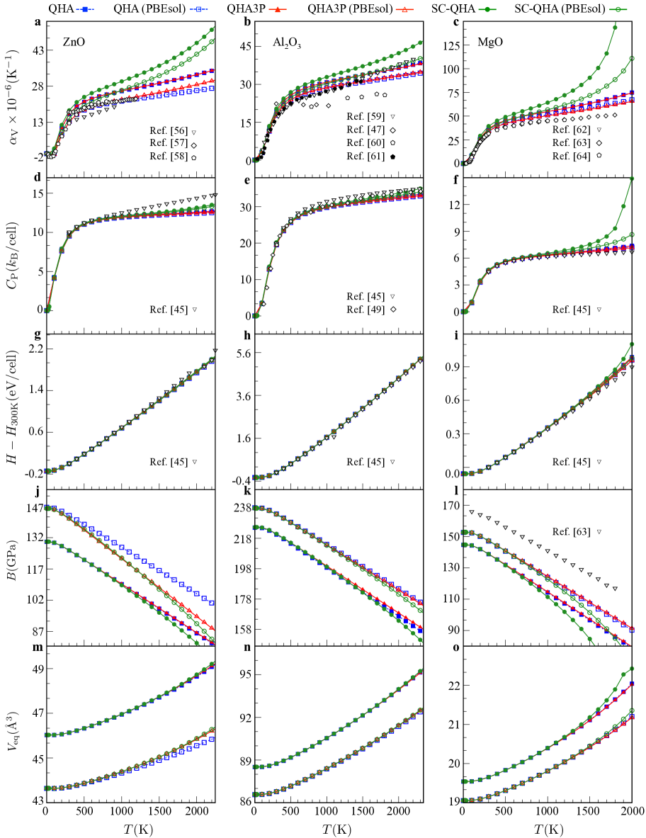
Figure 3: The thermodynamic properties of ZnO (a,d,g,j,m), Al₂O₃ (b,e,h,k,n), and MgO (c,f,i,l,o) as a function of temperature. The results of ZnO and Al₂O₃ are presented up to $T_{\scalebox{0.6}{m}}$, while MgO is shown up to $(2/3)T_{\rm m}$. The $T_{\scalebox{0.6}{m}}$ values of ZnO, Al₂O₃ and MgO are $2248$, $2345$ and $3125$ K Barin_1993 , respectively. The results are obtained with QHA3P, QHA and SC-QHA using the PBE and PBEsol XC functionals. Experimental results from different sources Khan_ACTACRIST_1986 ; Touloukian_NY_1977 ; Ibach_PSS_1972 ; Kondo_JPNJAP_2008 ; Yim_JAP_1978 ; Munro_JACERS_1997 ; Wachtman_JACERS_1962 ; Madelung_Springer_1999 ; Anderson_RGP_1992 ; White_JAP_1996 ; Barin_1993 are indicated by inverted triangles, diamonds, pentagons, and filled pentagons.

QHA3P Methodology. The QHA3P method requires only three phonon calculations along with the ${\sim}10$ $E_{\begin{subarray}{c}\scalebox{0.6}{0}\end{subarray}}$ energies. The Taylor expansion (Eq. 13) introduced in SC-QHA Huang_cms_2016 , is used to extrapolate the phonon spectra to the remaining volumes. The following steps are the same as QHA: fit to the EOS, minimize $F$ with respect to $V$, and calculate the thermodynamic properties (Figure 1a).

Although the same technique is used to extrapolate the phonon frequencies (Eq. (13)) in both QHA3P and SC-QHA, the definitions of some thermodynamic properties and the method of computing them are different. For example, the mode Grüneisen in QHA3P is calculated using Eq. (9), whereas in SC-QHA it is obtained using Eq. (14). In SC-QHA, $\gamma_{j}({\bf q})$ is temperature dependent, whereas it is temperature independent in QHA3P and QHA.

Implications of T dependent $\gamma_{j}({\bf q})$ in SC-QHA. The main contribution to Eq. (14) comes from $V_{{{\begin{subarray}{c}\scalebox{0.6}{eq}\end{subarray}}}}$, $\omega_{j}({\bf q})$, and $\left(\partial\omega_{j}({\bf q})/\partial V\right)_{{\begin{subarray}{c}\scalebox{0.6}{V}\end{subarray}}_{{\begin{subarray}{c}\scalebox{0.6}{0}\end{subarray}}}}$. The second term is neglected due to the small size of $\left(\partial^{2}\omega_{j}({\bf q})/\partial V^{2}\right)_{{\begin{subarray}{c}\scalebox{0.6}{V}\end{subarray}}_{{\begin{subarray}{c}\scalebox{0.6}{0}\end{subarray}}}}$.

• In SC-QHA, $\gamma_{j}({\bf q})$ is temperature dependent due to the prefactor $V_{\begin{subarray}{c}\scalebox{0.6}{eq}\end{subarray}}\left(T\right)/\omega_{j}\left({\bf q},V_{{{\begin{subarray}{c}\scalebox{0.6}{eq}\end{subarray}}}}\left(T\right)\right)$ (Eq. (14)).

• If $V_{{{\begin{subarray}{c}\scalebox{0.6}{eq}\end{subarray}}}}$ changes positively with $T$ and $\Big{(}\partial\omega_{j}({\bf q})/\partial V\Big{)}_{{\begin{subarray}{c}\scalebox{0.6}{V}\end{subarray}}_{{\begin{subarray}{c}\scalebox{0.6}{0}\end{subarray}}}}<0$, then $\gamma_{j}({\bf q})$ increases with $T$ (Eq. (14)).

• $\omega_{j}\left({\bf q},V_{{{\begin{subarray}{c}\scalebox{0.6}{eq}\end{subarray}}}}\left(T\right)\right)$ should decrease with increasing $T$ if the above condition is valid (Eq. (13)), amplifying the $T$ dependence of $\gamma_{j}({\bf q})$.

• If $\gamma_{j}({\bf q})$ increases for the majority of (${\bf q},j$) in the Brillouin zone, then $\bar{\gamma}$ will be overestimated by SC-QHA in comparison to QHA3P and QHA.

• ${\left(\partial\omega_{j}({\bf q})/\partial V\right)}_{{\begin{subarray}{c}\scalebox{0.6}{V}\end{subarray}}_{{\begin{subarray}{c}\scalebox{0.6}{0}\end{subarray}}}}$ is negative when $\omega_{j}({\bf q})$ decreases with $T$. The behavior of ${\left(\partial\omega_{j}({\bf q})/\partial V\right)}_{{\begin{subarray}{c}\scalebox{0.6}{V}\end{subarray}}_{{\begin{subarray}{c}\scalebox{0.6}{0}\end{subarray}}}}$ is described by the following expressions vanRoekeghem_PRB_2016 :

$$\begin{split}\left.\frac{{\rm d}\omega_{j}({\bf q})}{{\rm d}T}\right|_{{\begin{subarray}{c}\scalebox{0.6}{P}\end{subarray}}}&=\left(\frac{\partial\omega_{j}({\bf q})}{\partial V}\right)_{P}\left.\frac{\partial V}{\partial T}\right|_{{\begin{subarray}{c}\scalebox{0.6}{P}\end{subarray}}}\\[5.0pt] \Rightarrow\left(\frac{\partial\omega_{j}({\bf q})}{\partial V}\right)_{{\begin{subarray}{c}\scalebox{0.6}{P}\end{subarray}}}&=\frac{1}{V\alpha_{\begin{subarray}{c}\scalebox{0.6}{V}\end{subarray}}}\left.\frac{{\rm d}\omega_{j}({\bf q)}}{{\rm d}T}\right|_{{\begin{subarray}{c}\scalebox{0.6}{P}\end{subarray}}}.\end{split}$$ (17)

Thus, SC-QHA always produces larger $\bar{\gamma}$ values than QHA3P and QHA for materials where $\omega_{j}({\bf q})$ decreases with $T$ for the majority of (${\bf q},j$), and that have positive thermal expansion. This applies to positive thermal expansion materials (all of the materials in this study). The effect of this on $\alpha_{\begin{subarray}{c}\scalebox{0.6}{V}\end{subarray}}$ is discussed in the next section.

The root-mean-square relative deviation. The root-mean-square relative deviation (RMSrD)

$$\chi\left({\small X},{\small Y}\right)=\sqrt{\frac{\sum_{i}^{N}\left(\frac{X_{i}-Y_{i}}{X_{i}}\right)^{2}}{N-1}}$$ (18)

is used to quantitatively compare the calculated thermodynamic properties between the various methods, and to validate the model against experiments. Here $\chi\left({\small X},{\small Y}\right)$ represents the RMSrD between $N$ data points obtained from methods $\small X$ and $\small Y$. Small values of $\chi\left({\small X},{\small Y}\right)$ indicate that $\small X$ and $\small Y$ produce statistically similar results.

Geometry optimization. All structures are fully relaxed using the high-throughput framework AFLOW, and density functional theory package VASP  kresse_vasp . Optimizations are performed following the AFLOW standard curtarolo:art104 . The projector augmented wave (PAW) pseudopotentials PAW and the XC functionals proposed by Perdew-Burke-Ernzerhof (PBE) PBE are used for all calculations, unless otherwise stated. To study functional effects and compare with previous SC-QHA results Huang_cms_2016 , calculations using the PBEsol functional Perdew_PRL_2008 are also carried out. A high energy cutoff (40$\%$ larger than the maximum recommended cutoff among all the species) and a k-point mesh of 8000 k-points per reciprocal atom are used to ensure the accuracy of the results. Primitive cells are fully relaxed until the energy difference between two consecutive ionic steps is smaller than $10^{-9}$ eV and forces on each atom are below $10^{-8}$ eV/$\rm{\AA}$.

Phonon calculations. Phonon calculations are carried out using the Automatic Phonon Library curtarolo:art119 ; curtarolo:art125 , as implemented in AFLOW, using VASP to obtain the interatomic force constants via the finite-displacements approach. The magnitude of this displacement is chosen as 0.015$\rm\AA$. Supercell size and the number of atoms in the supercell (supercell atoms) along with space group number (sg #) of each example curtarolo:art135 are listed in Table 1. Non-analytical contributions to the dynamical matrix are also included using the formulation developed by Wang et al. Wang2010 . Frequencies and other related phonon properties are calculated on a 31$\times$31$\times$31 mesh in the Brillouin zone: sufficient to converge the vibrational density of states and thus the corresponding thermodynamic properties. The phonon density of states is calculated using the linear interpolation tetrahedron technique available in AFLOW.

The QHA calculations are performed on 10 equally spaced volumes ranging from ${-}3\%$ to $6\%$ uniform strain with $1\%$ increments from the respective equilibrium structures of the crystal. More expanded volumes are used since most materials have positive thermal expansion. Both the SC-QHA and the QHA3P calculations are performed using $\pm 3\%$ expanded and compressed volumes. All calculations are performed without external pressure ($P$=0), and all volume distortions are isotropic.

Table 1: Compound names with ICSD number, supercell size, supercell atoms, lattice type, and sg #. More detailed information is available in Table A1 Appendix.

compound	ICSD	supercell size	supercell atoms	lattice type	sg #
Si	76268	5$\times$5$\times$5	250	fcc	227
C (Diamond)	28857	4$\times$4$\times$4	128	fcc	227
SiC	618777	4$\times$4$\times$3	192	hex	186
Al2O3	89664	2$\times$2$\times$2	80	rhl	167
MgO	159372	4$\times$4$\times$4	128	fcc	225
ZnO	182356	4$\times$4$\times$3	192	hex	186
AlNi	602150	4$\times$4$\times$4	128	cub	221
NiTiSn	174568	3$\times$3$\times$3	81	fcc	216
Ti2AlN	157766	4$\times$4$\times$1	128	hex	194

Table 2: RMSrD for $\alpha_{\scalebox{0.6}{V}}$ for all non-metallic materials. $\chi$ for $\alpha_{\scalebox{0.6}{V}}$ are calculated with respect to the experiments in: Ref. Okada_JAP_1984 (Si), Ref. Slack_JAP_1975 (C), Ref. Li_JAP_1986 (SiC), Ref. Touloukian_NY_1977 (ZnO), Ref. Kondo_JPNJAP_2008 (Al₂O₃), and Ref. Anderson_RGP_1992 (MgO). Units: RMSrD in %.

	$\chi({\scalebox{0.6}{QHA3P}},{\scalebox{0.6}{QHA}})$ %	$\chi({\scalebox{0.6}{SC-QHA}},{\scalebox{0.6}{QHA}})$ %	$\chi({\scalebox{0.6}{QHA3P}},{\scalebox{0.6}{expt}})$ %	$\chi({\scalebox{0.6}{SC-QHA}},{\scalebox{0.6}{expt}})$ %
	($\alpha_{\begin{subarray}{c}\scalebox{0.6}{V}\end{subarray}}$)	($\alpha_{\begin{subarray}{c}\scalebox{0.6}{V}\end{subarray}}$)	($\alpha_{\begin{subarray}{c}\scalebox{0.6}{V}\end{subarray}}$)	($\alpha_{\begin{subarray}{c}\scalebox{0.6}{V}\end{subarray}}$)
compound	PBE   PBEsol	PBE   PBEsol	PBE   PBEsol	PBE   PBEsol
Si	0.1      1.3	9.2      7.5	15.7      8.4	25.8     19.6
C	0.8      1.0	2.8      4.5	14.0     12.1	16.8     12.4
SiC	0.7      0.4	4.7      3.7	13.5     12.7	12.6     11.1
ZnO	0.4      5.9	27.0     37.7	16.7      7.3	31.7     16.2
Al2O3	0.3      0.8	11.1      9.5	12.4      8.1	18.7      9.1
MgO	0.1      1.8	27.5     14.5	25.4     14.4	75.0     38.0

Table 3: RMSrD for $\alpha_{\scalebox{0.6}{V}}$, $C_{\scalebox{0.6}{P}}$, and $H$ for metallic materials and a small band gap compound. $\chi$ for $\alpha_{\scalebox{0.6}{V}}$ are computed with respect to the experiment in Refs: Wang_ACTAMAT_2004 (AlNi), Ref. Hermet_JPCC_2014 (NiTiSn), and Ref. Drulis_JAC_2007 (Ti₂AlN). Units: RMSrD in %.

Compound	$\chi({\scalebox{0.6}{QHA3P}},{\scalebox{0.6}{expt}})$ %	$\chi({\scalebox{0.6}{QHA3P}},{\scalebox{0.6}{expt}})$ %	$\chi({\scalebox{0.6}{QHA3P}},{\scalebox{0.6}{expt}})$ %	$\chi({\scalebox{0.6}{QHA3P}},{\scalebox{0.6}{expt}})$ %	$\chi({\scalebox{0.6}{QHA3P}},{\scalebox{0.6}{expt}})$ %	$\chi({\scalebox{0.6}{QHA3P}},{\scalebox{0.6}{expt}})$ %
	($\alpha_{{\begin{subarray}{c}\scalebox{0.6}{V}\end{subarray}},{\begin{subarray}{c}\scalebox{0.6}{ph+elec}\end{subarray}}}$)	($\alpha_{\begin{subarray}{c}\scalebox{0.6}{V}\end{subarray}}$)	($C_{{\begin{subarray}{c}\scalebox{0.6}{P}\end{subarray}},{\begin{subarray}{c}\scalebox{0.6}{ph+elec}\end{subarray}}}$)	($C_{{\begin{subarray}{c}\scalebox{0.6}{P}\end{subarray}}}$)	($H_{{\begin{subarray}{c}\scalebox{0.6}{ph+elec}\end{subarray}}}$)	($H$)
AlNi	5.2	5.1	2.6	3.2	5.6	1.9
NiTiSn	6.4	6.2	0.0	0.0	n/a	n/a
Ti2AlN	4.9	5.7	0.0	0.0	n/a	n/a

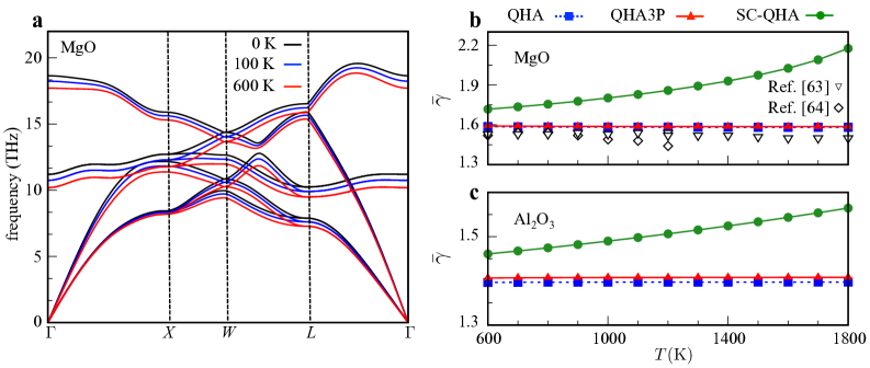
Figure 4: (a) The phonon dispersion curves of MgO at three different temperatures are computed using SC-QHA equilibrium volumes and Eq. (13). (b, c) The $\bar{\gamma}$ values as a function of temperature for MgO and Al₂O₃ using QHA3P, QHA  and SC-QHA. The experimental Grüneisen parameters of MgO are taken from Ref. White_JAP_1996 ; Anderson_RGP_1992 .

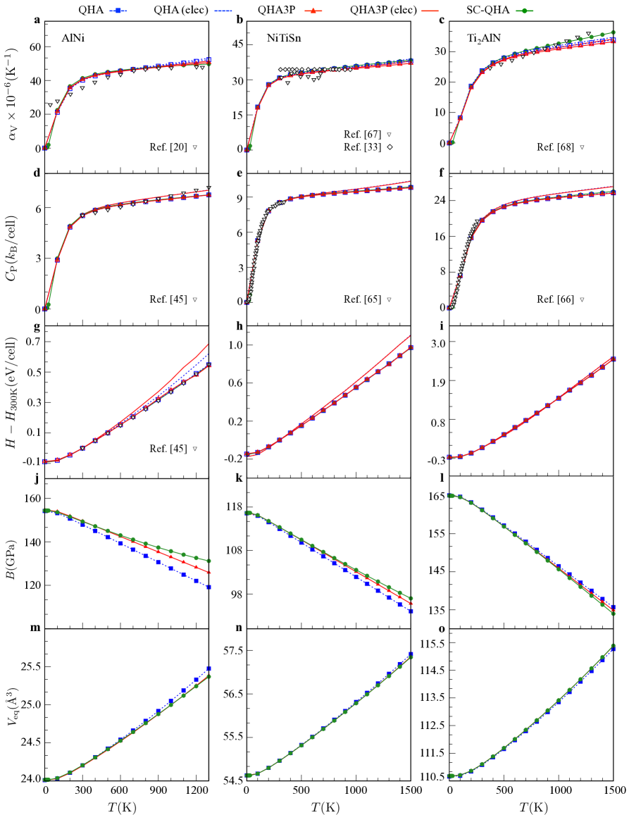
Figure 5: The thermodynamic properties of AlNi (a,d,g,j,m), NiTiSn (b,e,h,k,n), and Ti₂AlN (c,f,i,l,o) are shown up to the respective $T_{\scalebox{0.6}{m}}$ of $1300$ K, $1500$ K and $1500$ K Wang_ACTAMAT_2004 ; Jung_JAC_2010 ; Hermet_JPCC_2014 ; Lane_JCCERS_2011 ; Drulis_JAC_2007 , respectively. QHA3P results are compared with QHA and experiments. Experimental results from different sources Wang_ACTAMAT_2004 ; Jung_JAC_2010 ; Hermet_JPCC_2014 ; Lane_JCCERS_2011 ; Drulis_JAC_2007 ; Barin_1993 are indicated by inverted triangles and diamonds.

Results and Discussion

Thermodynamic properties of non-metallic materials from the three approaches are compared, and the same methods are applied to metallic and small band gap materials.

Non-metallic compounds. The thermodynamic properties are illustrated in Figure 2 for Si, C, and SiC and in Figure 3 for ZnO, Al₂O₃, and MgO. Comparisons of QHA3P with QHA, SC-QHA, and experimental data are discussed below with two different XC functionals.

$\alpha_{\begin{subarray}{c}\scalebox{0.6}{V}\end{subarray}}$ from both QHA3P and QHA agree well with the available experiments for all tested non-metallic compounds using both XC functionals. Conversely, SC-QHA overestimates $\alpha_{\begin{subarray}{c}\scalebox{0.6}{V}\end{subarray}}$ for Si, ZnO, Al₂O₃, and MgO. Using the PBEsol XC functional improves consistency with experimental results for Si, however $\alpha_{\begin{subarray}{c}\scalebox{0.6}{V}\end{subarray}}$ is still larger for ZnO and MgO. For Al₂O₃, $\alpha_{\begin{subarray}{c}\scalebox{0.6}{V}\end{subarray}}$ values from different experiments  Kondo_JPNJAP_2008 ; Yim_JAP_1978 ; Munro_JACERS_1997 ; Wachtman_JACERS_1962 vastly differ from one other. Below $1500$ K, experimental results from Ref Kondo_JPNJAP_2008 ; Wachtman_JACERS_1962 are well described by PBEsol, whereas above $1500$ K, they are better predicted by PBE. The RMSrD between $\alpha_{\begin{subarray}{c}\scalebox{0.6}{V}\end{subarray}}$ from different approaches and experiment are provided in Table 2. The relatively small RMSrD between QHA3P and experiments compared to the RMSrD between SC-QHA and experiments indicate that the QHA3P $\alpha_{\begin{subarray}{c}\scalebox{0.6}{V}\end{subarray}}$ predictions are more reliable.

The larger values of $\alpha_{\begin{subarray}{c}\scalebox{0.6}{V}\end{subarray}}$ from SC-QHA are due to the overestimation of $\bar{\gamma}$. This is particularly significant for positive $\alpha_{\begin{subarray}{c}\scalebox{0.6}{V}\end{subarray}}$ materials, where $\omega_{j}({\bf q})$ decreases with $T$ for almost all (${\bf q},j$) (QHA3P Methodology section). For example, the $T$ dependent phonon dispersion curves of MgO (Figure 4(a)) show that $\omega_{j}({\bf q})$ decreases for all (${\bf q},j$), except for the acoustic branches near $\Gamma$. The $\bar{\gamma}$ values for MgO along with Al₂O₃ are illustrated in Figure 4(b, c), and are validated by experiments.

Despite differences in $\alpha_{\begin{subarray}{c}\scalebox{0.6}{V}\end{subarray}}$, there are no significant differences between $C_{{\begin{subarray}{c}\scalebox{0.6}{P}\end{subarray}}}$ and $H$ obtained from the three approaches. The values are insensitive to the choice of functional, except for MgO (Figure 2 and 3(d-i)). Both $C_{{\begin{subarray}{c}\scalebox{0.6}{P}\end{subarray}}}$ and $H$ match well with the experimental values. A slight underestimation is observed for $C_{{\begin{subarray}{c}\scalebox{0.6}{P}\end{subarray}}}$ for Si, SiC, and ZnO. Also, divergence from experiments occurs near $2000$ K for MgO using the PBE XC functional in SC-QHA. The observations are supported by the RMSrD of $C_{{\begin{subarray}{c}\scalebox{0.6}{P}\end{subarray}}}$ (Table A2, Appendix).

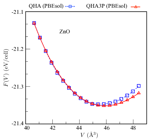
Figure A1: $F{-}V$ curve of ZnO. The $F(V)$ curve of ZnO at $2000$ K. The range of volume is from $-6$ to $12$ percent of $V_{\scalebox{0.6}{0}}$ ($43.22$ ų). The difference between the two curves gives $F_{\scalebox{0.6}{vib}}$, since $E_{\scalebox{0.6}{0}}$ is the same for both QHA and QHA3P.

The values of $B$ computed with the three methodologies also match when using the same XC functional, except for ZnO and MgO (Figure 2 and 3(j-o)). For ZnO, discrepancies are observed between the QHA3P and QHA results. Since the bulk modulus value is related to the curvature of $F(V)$ at $V_{\begin{subarray}{c}\scalebox{0.6}{eq}\end{subarray}}$, any small change in $F(V)$ leads to a larger change in $B$. For instance, at $2000$ K the difference in $F$ between QHA3P and QHA for ZnO is approximately $5$ meV at $6\%$ expanded volume of $V_{\begin{subarray}{c}\scalebox{0.6}{0}\end{subarray}}$ (Figure A1, Appendix), which significantly affects $B$ (Figure 3(j)). The values of $B$ calculated using PBEsol are larger than for PBE, with similar trends previously reported elsewhere Csonka_PRB_2009 , and are closer to experiment. For MgO, some deviation occurs at high temperature between SC-QHA and QHA3P (and QHA). RMSrD with experiment for $B$ has not been calculated due to limited data availability. For $B$, the small RMSrD values between QHA3P and QHA demonstrate that the methods are consistent with each other. The RMSrD values between SC-QHA and QHA are high for ZnO and MgO (Table A2, Appendix).

As for $B$, predicted $V_{\begin{subarray}{c}\scalebox{0.6}{eq}\end{subarray}}$ values are similar for all of the methods when using the same XC functional. However, the volume predictions obtained using PBEsol are smaller than those for PBE (Figure 2 and 3(m-o)).

Metallic compounds and narrow band gap materials. The thermodynamic properties of the metals AlNi and Ti₂AlN and the narrow band gap ($0.12$ eV Aliev_PBCM_1990 ) half-Heusler NiTiSn are presented in Figure 5. For QHA3P and QHA, calculations are performed with and without the electronic contribution. Results for SC-QHA are presented without the electronic contribution, since it is not implemented in AFLOW for this method. In this section calculations are performed only with the PBE XC functional.

Similar to the non-metallic examples, there are no prominent differences between $\alpha_{\begin{subarray}{c}\scalebox{0.6}{V}\end{subarray}}$ obtained using these three methods (Figure 5(a-c)). The $\alpha_{\begin{subarray}{c}\scalebox{0.6}{V}\end{subarray}}$ results show the effectiveness of all methodologies in accurately predicting the experimental thermodynamic properties of AlNi, NiTiSn, and Ti₂AlN. In addition, the contribution of $F_{{\begin{subarray}{c}\scalebox{0.6}{elec}\end{subarray}}}$ to $F$ does not alter the results.

The other thermodynamic properties, $C_{{\begin{subarray}{c}\scalebox{0.6}{P}\end{subarray}}}$, $H$, $B$, and $V_{\begin{subarray}{c}\scalebox{0.6}{eq}\end{subarray}}$, also match well with each other for these three methods and with experiments, with a few exceptions (Figure 5(d-f)). The $H$ values for AlNi from QHA3P and QHA do not agree with experiments above 500 K when $F_{{\begin{subarray}{c}\scalebox{0.6}{elec}\end{subarray}}}$ is taken into consideration (Figure 5(g, j)). The $B$ values from the three methods show discrepancies stemming from the difference in the $F(V)$ energies as described in the non-metallic compounds section. The small RMSrD between QHA3P and experiment for $\alpha_{\begin{subarray}{c}\scalebox{0.6}{V}\end{subarray}}$, $C_{{\begin{subarray}{c}\scalebox{0.6}{P}\end{subarray}}}$, and $H$ indicate that the results agree well with experiments (Table 3). Since the QHA, SC-QHA, and QHA3P predictions are similar, RMSrD values are presented only for QHA3P.

Conclusions

The quasi-harmonic approximation 3-phonons method is introduced to calculate thermodynamic properties of both non-metallic and metallic compounds. The efficiency of QHA3P is tested for a range of materials using two different exchange-correlation functionals, and the calculated thermodynamic quantities are in agreement with both QHA and experimental measurements. We also show that SC-QHA overestimates the average Grüneisen parameter, as well as $\alpha_{\begin{subarray}{c}\scalebox{0.6}{V}\end{subarray}}$, at high temperatures for some materials, while QHA3P still performs well. This study demonstrates that QHA3P is an ideal framework for the high-throughput prediction of finite temperature materials properties, combining the accuracy of QHA with the computational efficiency of SC-QHA.
 

Appendix

Table A1: List of crystallographic properties. List of compound names with various crystallographic properties along with AFLOW prototype curtarolo:art121 ; Hicks_arXiv_2018 and AFLOW unique identifier (auid) curtarolo:art128 .

compound	ICSD	supercell size	supercell atoms	lattice type	sg#	DFT band gap (eV)	prototype	auid
Si	76268	5$\times$5$\times$5	250	fcc	227	0.61	A_cF8_227_a A_cF8_227_a	aflow:ff211836be789f69
C (Diamond)	28857	4$\times$4$\times$4	128	fcc	227	4.11	A_cF8_227_a A_cF8_227_a	aflow:b438e1a25f9c187d
SiC	618777	4$\times$4$\times$3	192	hex	186	2.30	AB_hP4_186_b_b AB_hP4_186_b_b	aflow:50.644a24702c7dc
ZnO	182356	4$\times$4$\times$3	192	hex	186	1.81	AB_hP4_186_b_b AB_hP4_186_b_b	aflow:f30df164c6192045
Al2O3	89664	2$\times$2$\times$2	80	rhl	167	5.86	A2B3_hR10_167_c_e A2B3_hR10_167_c_e	aflow:537e800e0a1b75be
MgO	159372	4$\times$4$\times$4	128	fcc	225	4.46	AB_cF8_225_a_b AB_cF8_225_a_b	aflow:a2cc05c200330e16
AlNi	602150	4$\times$4$\times$4	128	cub	221	0.00	AB_cP2_221_b_a AB_cP2_221_b_a	aflow:f727dcd6a292301d
NiTiSn	174568	3$\times$3$\times$3	81	fcc	216	0.17	ABC_cF12_216_b_c_a ABC_cF12_216_b_c_a	aflow:7bed936e9d5a44ca
Ti2AlN	157766	4$\times$4$\times$1	128	hex	194	0.00	ABC2_hP8_194_d_a_f ABC2_hP8_194_d_a_f	aflow:bdc38ae3ca07e398

Table A2: List of RMSrD values. RMSrD for $C_{\scalebox{0.6}{P}}$, and $B$ for all non-metallic materials. $\chi$ for $C_{\scalebox{0.6}{P}}$ are calculated with respect to the experiments in: Ref. Barin_1993 . $\chi$ for $H$ and $V_{\scalebox{0.6}{eq}}$ are similar to $C_{\scalebox{0.6}{P}}$ and $B$, respectively, and are not presented. Units: RMSrD in %.

	$\chi({\scalebox{0.6}{QHA3P}},{\scalebox{0.6}{expt}})$ %	$\chi({\scalebox{0.6}{SC-QHA}},{\scalebox{0.6}{expt}})$ %	$\chi({\scalebox{0.6}{QHA3P}},{\scalebox{0.6}{QHA}})$ %	$\chi({\scalebox{0.6}{SC-QHA}},{\scalebox{0.6}{QHA}})$ %
	($C_{\begin{subarray}{c}\scalebox{0.6}{P}\end{subarray}}$)	($C_{\begin{subarray}{c}\scalebox{0.6}{P}\end{subarray}}$)	($B$)	($B$)
compound	PBE   PBEsol	PBE   PBEsol	PBE   PBEsol	PBE   PBEsol
Si	7.4     7.6	7.1     7.7	0.5     0.2	0.2     0.4
C	2.2     2.2	3.1     1.8	0.5     0.0	1.0     0.5
SiC	4.8     5.0	4.4     4.6	0.0     0.1	0.2     0.3
ZnO	8.5     9.3	5.9     7.0	0.3     7.0	3.4     9.8
Al2O3	4.5     5.3	3.0     4.1	0.8     0.3	1.1     1.7
MgO	9.0     3.6	37.1    11.5	0.5     0.7	21.6     6.6

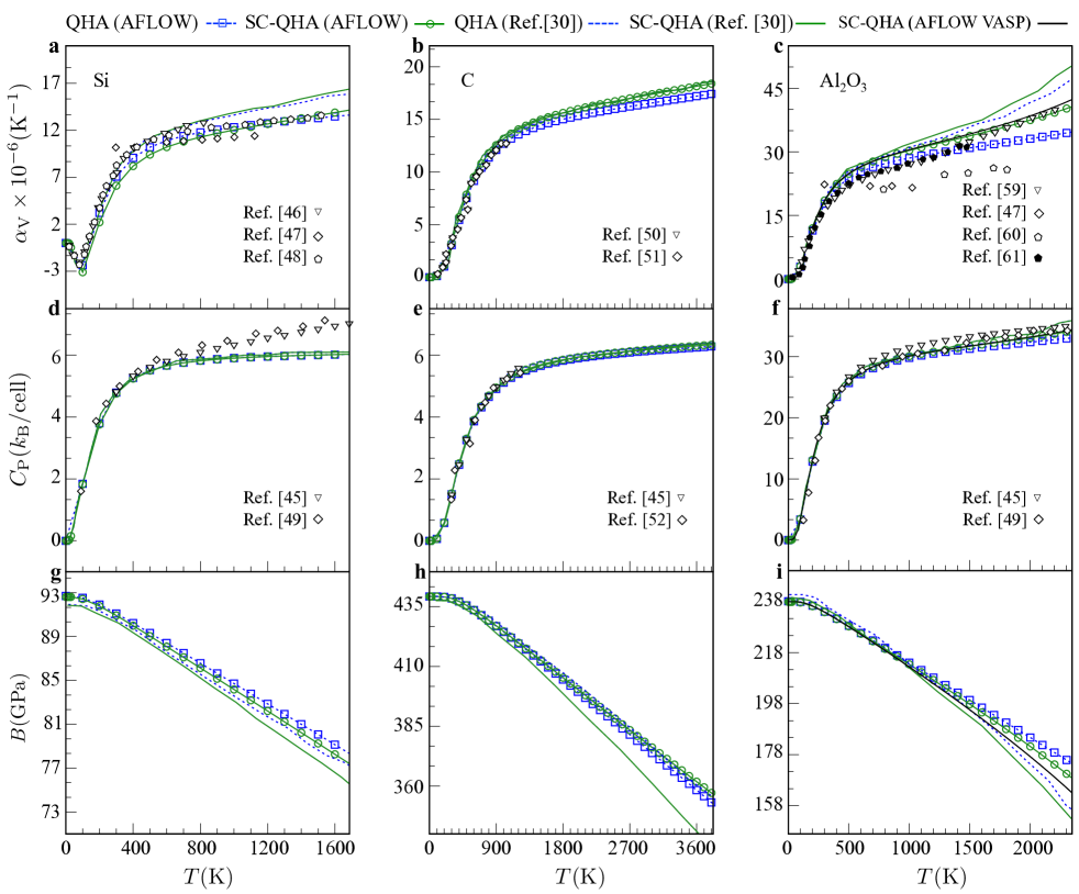
Figure A2: The comparison of AFLOW computed $\alpha_{\scalebox{0.6}{V}}$, $C_{\scalebox{0.6}{P}}$ and $B$ with Ref. Huang_cms_2016 . Experimental results from different sources Gibbons_PR_1958 ; Yim_JAP_1978 ; Okada_JAP_1984 ; Kondo_JPNJAP_2008 ; Skinner_AM_1957 ; Slack_JAP_1975 ; Barin_1993 ; Victor_JCP_1962 ; Li_JAP_1986 ; Wachtman_JACERS_1962 ; Munro_JACERS_1997 ; Anderson_RGP_1992 ; Chase_AIP_1998 ; Barin_1993 are indicated by inverted triangles, diamonds, pentagons and filled pentagons. The black colored line for Al₂O₃ represents calculations with the PHONOPY+SC-QHA codes Togo_prb_2015 ; Huang_cms_2016 , performed using the AFLOW standard VASP input parameters.

Comparison of SC-QHA from AFLOW and Ref. Huang_cms_2016 . The SC-QHA method was originally developed and tested in Ref. Huang_cms_2016 using the PBEsol XC functional. To check the consistency between the AFLOW implementation of SC-QHA and Ref. Huang_cms_2016 , the calculated properties are compared for Si, C, and Al₂O₃. The differences between the properties computed with AFLOW and Ref. Huang_cms_2016 are marginal. However, some discrepancies are observed for the $\alpha_{\begin{subarray}{c}\scalebox{0.6}{V}\end{subarray}}$ values of Si, $B$ values of C, and the $\alpha_{\begin{subarray}{c}\scalebox{0.6}{V}\end{subarray}}$ and $B$ values of Al₂O₃, which are the presented examples in Ref. Huang_cms_2016 . To investigate this, thermodynamic properties are reproduced for Al₂O₃ using the original SC-QHA and PHONOPY Togo_prb_2015 codes with the AFLOW standard VASP input parameters (Figure A2, Appendix). This indicates that the origin of the incompatibility between these two studies is the difference in the VASP input parameters. While the accuracy is increased by using the AFLOW standard VASP input parameters, the results are still inconsistent with experiments and QHA.

References

- (1) S. Curtarolo, W. Setyawan, G. L. W. Hart, M. Jahnátek, R. V. Chepulskii, R. H. Taylor, S. Wang, J. Xue, K. Yang, O. Levy, M. J. Mehl, H. T. Stokes, D. O. Demchenko, and D. Morgan, AFLOW: An automatic framework for high-throughput materials discovery, Comput. Mater. Sci. 58, 218–226 (2012).
- (2) S. Curtarolo, W. Setyawan, S. Wang, J. Xue, K. Yang, R. H. Taylor, L. J. Nelson, G. L. W. Hart, S. Sanvito, M. Buongiorno Nardelli, N. Mingo, and O. Levy, AFLOWLIB.ORG: A distributed materials properties repository from high-throughput ab initio calculations, Comput. Mater. Sci. 58, 227–235 (2012).
- (3) R. H. Taylor, F. Rose, C. Toher, O. Levy, K. Yang, M. Buongiorno Nardelli, and S. Curtarolo, A RESTful API for exchanging materials data in the AFLOWLIB.org consortium, Comput. Mater. Sci. 93, 178–192 (2014).
- (4) A. R. Supka, T. E. Lyons, L. S. I. Liyanage, P. D’Amico, R. Al Rahal Al Orabi, S. Mahatara, P. Gopal, C. Toher, D. Ceresoli, A. Calzolari, S. Curtarolo, M. Buongiorno Nardelli, and M. Fornari, AFLOW: A minimalist approach to high-throughput ab initio calculations including the generation of tight-binding hamiltonians, Comput. Mater. Sci. 136, 76–84 (2017).
- (5) F. Rose, C. Toher, E. Gossett, C. Oses, M. Buongiorno Nardelli, M. Fornari, and S. Curtarolo, AFLUX: The LUX materials search API for the AFLOW data repositories, Comput. Mater. Sci. 137, 362–370 (2017).
- (6) H. Yu, D. Duan, H. Liu, T. Yang, F. Tian, K. Bao, D. Li, Z. Zhao, B. Liu, and T. Cui, Ab initio molecular dynamic study of solid-state transitions of ammonium nitrate, Sci. Rep. 6, 18918 (2016).
- (7) G. Kresse and J. Hafner, Ab initio molecular dynamics for open-shell transition metals, Phys. Rev. B 48, 13115–13118 (1993).
- (8) J. Sarnthein, K. Schwarz, and P. E. Blöchl, Ab initio molecular-dynamics study of diffusion and defects in solid Li3N, Phys. Rev. B 53, 9084–9091 (1996).
- (9) H. L. Zhang, Y. F. Han, W. Zhou, Y. B. Dai, J. Wang, and B. D. Sun, Atomic study on the ordered structure in Al melts induced by liquid/substrate interface with Ti solute, Appl. Phys. Lett. 106, 041606 (2015).
- (10) B. J. Jesson and P. A. Madden, Structure and dynamics at the aluminum solid-liquid interface: An ab initio simulation, J. Chem. Phys. 113, 5935–5946 (2000).
- (11) I. Errea, M. Calandra, and F. Mauri, First-Principles Theory of Anharmonicity and the Inverse Isotope Effect in Superconducting Palladium-Hydride Compounds, Phys. Rev. Lett. 111, 177002 (2013).
- (12) I. Errea, M. Calandra, and F. Mauri, Anharmonic free energies and phonon dispersions from the stochastic self-consistent harmonic approximation: Application to platinum and palladium hydrides, Phys. Rev. B 89, 064302 (2014).
- (13) M. A. Blanco, E. Francisco, and V. Luaña, GIBBS: isothermal-isobaric thermodynamics of solids from energy curves using a quasi-harmonic Debye model, Comput. Phys. Commun. 158, 57–72 (2004).
- (14) J.-P. Poirier, Introduction to the Physics of the Earth’s Interior (Cambridge University Press, 2000), 2nd edn.
- (15) O. Isayev, C. Oses, C. Toher, E. Gossett, S. Curtarolo, and A. Tropsha, Universal fragment descriptors for predicting electronic properties of inorganic crystals, Nat. Commun. 8, 15679 (2017).
- (16) E. Gossett, C. Toher, C. Oses, O. Isayev, F. Legrain, F. Rose, E. Zurek, J. Carrete, N. Mingo, A. Tropsha, and S. Curtarolo, AFLOW-ML: A RESTful API for machine-learning predictions of materials properties, Comput. Mater. Sci. 152, 134–145 (2018).
- (17) C. Toher, J. J. Plata, O. Levy, M. de Jong, M. D. Asta, M. Buongiorno Nardelli, and S. Curtarolo, High-throughput computational screening of thermal conductivity, Debye temperature, and Grüneisen parameter using a quasiharmonic Debye model, Phys. Rev. B 90, 174107 (2014).
- (18) C. Toher, C. Oses, J. J. Plata, D. Hicks, F. Rose, O. Levy, M. de Jong, M. D. Asta, M. Fornari, M. Buongiorno Nardelli, and S. Curtarolo, Combining the AFLOW GIBBS and Elastic Libraries to efficiently and robustly screen thermomechanical properties of solids, Phys. Rev. Mater. 1, 015401 (2017).
- (19) Z. K. Liu and Y. Wang, Computational Thermodynamics of Materials (Cambridge University Press, 2016), 1 edn.
- (20) Y. Wang, Z.-K. Liu, and L.-Q. Chen, Thermodynamic properties of Al, Ni, NiAl, and Ni3Al from first-principles calculations, Acta Mater. 52, 2665–2671 (2004).
- (21) T. Duong, S. Gibbons, R. Kinra, and R. Arróyave, Ab-initio approach to the electronic, structural, elastic, and finite-temperature thermodynamic properties of Ti ( = Al or Ga and = C or N), J. Appl. Phys. 110, 093504 (2011).
- (22) P. Nath, J. J. Plata, D. Usanmaz, R. Al Rahal Al Orabi, M. Fornari, M. Buongiorno Nardelli, C. Toher, and S. Curtarolo, High-throughput prediction of finite-temperature properties using the quasi-harmonic approximation, Comput. Mater. Sci. 125, 82–91 (2016).
- (23) J. M. Ziman, Electrons and Phonons: The Theory of Transport Phenomena in Solids, Oxford Classic Texts in the Physical Sciences (Oxford University Press, 1960).
- (24) D. C. Wallace, Thermodynamics of crystals (Wiley, 1972).
- (25) M. T. Dove, Introduction to Lattice Dynamics, Cambridge Topics in Mineral Physics and Chemistry (Cambridge University Press, 1993).
- (26) G. P. Srivastava, The Physics of Phonons (CRC Press, Taylor & Francis, 1990).
- (27) S. Baroni, S. de Gironcoli, A. Dal Corso, and P. Giannozzi, Phonons and related crystal properties from density-functional perturbation theory, Rev. Mod. Phys. 73, 515–562 (2001).
- (28) A. van de Walle and G. Ceder, The effect of lattice vibrations on substitutional alloy thermodynamics, Rev. Mod. Phys. 74, 11–45 (2002).
- (29) J. J. Plata, P. Nath, D. Usanmaz, J. Carrete, C. Toher, M. de Jong, M. D. Asta, M. Fornari, M. Buongiorno Nardelli, and S. Curtarolo, An efficient and accurate framework for calculating lattice thermal conductivity of solids: AFLOW-AAPL Automatic Anharmonic Phonon Library, NPJ Comput. Mater. 3, 45 (2017).
- (30) L.-F. Huang, X.-Z. Lu, E. Tennessen, and J. M. Rondinelli, An efficient ab-initio quasiharmonic approach for the thermodynamics of solids, Comput. Mater. Sci. 120, 84–93 (2016).
- (31) R. Arroyave, D. Shin, and Z.-K. Liu, Ab initio thermodynamic properties of stoichiometric phases in the Ni-Al system, Acta Mater. 53, 1809–1819 (2005).
- (32) T. Tohei, Y. Watanabe, H.-S. Lee, and Y. Ikuhara, First principles calculation of thermal expansion coefficients of pure and Cr doped -alumina crystals, J. Appl. Phys. 120, 142106 (2016).
- (33) P. Hermet, R. M. Ayral, E. Theron, P. G. Yot, F. Salles, M. Tillard, and P. Jund, Thermal Expansion of Ni-Ti-Sn Heusler and Half-Heusler Materials from First-Principles Calculations and Experiments, J. Phys. Chem. C 118, 22405–22411 (2014).
- (34) C.-L. Fu and K.-M. Ho, First-principles calculation of the equilibrium ground-state properties of transition metals: Applications to Nb and Mo, Phys. Rev. B 28, 5480–5486 (1983).
- (35) J. Sólyom, Fundamentals of the physics of solids, vol. 1 (Springer Berlin Heidelberg, 2007), 1 edn.
- (36) I. Barin, Thermochemical Data of pure substances (VCH, Germany, 1993).
- (37) D. F. Gibbons, Thermal Expansion of Some Crystals with the Diamond Structure, Phys. Rev. 112, 136–140 (1958).
- (38) W. M. Yim and R. J. Paff, Thermal expansion of AlN, sapphire, and silicon, J. Appl. Phys. 45, 1456–1457 (1974).
- (39) Y. Okada and Y. Tokumaru, Precise determination of lattice parameter and thermal expansion coefficient of silicon between 300 and 1500 K, J. Appl. Phys. 56, 314–320 (1984).
- (40) M. W. Chase Jr., NIST-JANAF Thermochemical Tables, Journal of Physical and Chemical Reference Data Monographs (American Inst. of Physics, 1998), fourth edition edn.
- (41) G. A. Slack and S. F. Bartram, Thermal expansion of some diamond-like crystals, J. Appl. Phys. 46, 89–98 (1975).
- (42) B. J. Skinner, The thermal expansion of theoria, periclase, and diamond, Am. Mineral. 42, 39–55 (1957).
- (43) A. C. Victor, Heat Capacity of Diamond at High Temperatures, J. Chem. Phys. 36, 1903–1911 (1962).
- (44) H. J. McSkimin and P. Andreatch Jr., Elastic Moduli of Diamond as a Function of Pressure and Temperature, J. Appl. Phys. 43, 2944–2948 (1972).
- (45) Z. Li and R. C. Bradt, Thermal expansion of the hexagonal (4H) polytype of SiC, J. Appl. Phys. 60, 612–614 (1986).
- (46) G. I. Csonka, J. P. Perdew, A. Ruzsinszky, P. H. T. Philipsen, S. Lebègue, J. Paier, O. A. Vydrov, and J. G. Ángyán, Assessing the Performance of Recent Density Functionals for Bulk Solids, Phys. Rev. B 79, 155107 (2009).
- (47) A. A. Khan, X-ray determination of thermal expansion of zinc oxide, Acta Crystallogr. Sect. A 24, 403 (1968).
- (48) Y. S. Touloukian, R. K. Kirby, R. E. Taylor, and P. D. Desai, Thermophysical Properties of Matter; Thermal Expansion; Nonmetallic Solids, vol. 13 (IFI-Plenum, New York, 1977).
- (49) H. Ibach, Thermal Expansion of Silicon and Zinc Oxide (II), Phys. Stat. Solidi 33, 257–265 (1969).
- (50) S. Kondo, K. Tateishi, and N. Ishizawa, Structural Evolution of Corundum at High Temperatures, Jpn. J. Appl. Phys. 47, 616 (2008).
- (51) R. G. Munro, Evaluated Material Properties for a Sintered -Alumina, J. Am. Ceram. Soc. 80, 1919–1928 (1997).
- (52) J. B. Wachtman Jr., T. G. Scuderi, and G. W. Cleek, Linear Thermal Expansion of Aluminum Oxide and Thorium Oxide from 100∘ to 1100∘K, J. Am. Ceram. Soc. 45, 319–323 (1962).
- (53) O. Madelung, U. Rössler, and M. Schulz, eds., II-VI and I-VII Compounds; Semimagnetic Compounds (Springer Berlin Heidelberg, Berlin, Heidelberg, 1999), doi:10.1007/b71137.
- (54) O. L. Anderson, D. Isaak, and H. Oda, High-temperature elastic constant data on minerals relevant to geophysics, Rev. Geophys. 30, 57–90 (1992).
- (55) G. K. White and O. L. Anderson, Grüneisen Parameter of Magnesium Oxide, J. Appl. Phys. 37, 430–432 (1966).
- (56) A. van Roekeghem, J. Carrete, and N. Mingo, Anomalous thermal conductivity and suppression of negative thermal expansion in ScF3, Phys. Rev. B 94, 020303(R) (2016).
- (57) G. Kresse and J. Hafner, Ab initio molecular dynamics for liquid metals, Phys. Rev. B 47, 558–561 (1993).
- (58) C. E. Calderon, J. J. Plata, C. Toher, C. Oses, O. Levy, M. Fornari, A. Natan, M. J. Mehl, G. L. W. Hart, M. Buongiorno Nardelli, and S. Curtarolo, The AFLOW standard for high-throughput materials science calculations, Comput. Mater. Sci. 108 Part A, 233–238 (2015).
- (59) P. E. Blöchl, Projector augmented-wave method, Phys. Rev. B 50, 17953–17979 (1994).
- (60) J. P. Perdew, K. Burke, and M. Ernzerhof, Generalized Gradient Approximation Made Simple, Phys. Rev. Lett. 77, 3865–3868 (1996).
- (61) J. P. Perdew, A. Ruzsinszky, G. I. Csonka, O. A. Vydrov, G. E. Scuseria, L. A. Constantin, X. Zhou, and K. Burke, Restoring the Density-Gradient Expansion for Exchange in Solids and Surfaces, Phys. Rev. Lett. 100, 136406 (2008).
- (62) P. Nath, J. J. Plata, D. Usanmaz, C. Toher, M. Fornari, M. Buongiorno Nardelli, and S. Curtarolo, High throughput combinatorial method for fast and robust prediction of lattice thermal conductivity, Scr. Mater. 129, 88–93 (2017).
- (63) D. Hicks, C. Oses, E. Gossett, G. Gomez, R. H. Taylor, C. Toher, M. J. Mehl, O. Levy, and S. Curtarolo, AFLOW-SYM: platform for the complete, automatic and self-consistent symmetry analysis of crystals, Acta Crystallogr. Sect. A 74, 184–203 (2018).
- (64) Y. Wang, J. J. Wang, W. Y. Wang, Z. G. Mei, S. L. Shang, L. Q. Chen, and Z. K. Liu, A mixed-space approach to first-principles calculations of phonon frequencies for polar materials, J. Phys.: Condens. Matter 22, 202201 (2010).
- (65) M. K. Drulis, H. Drulis, A. E. Hackemer, A. Ganguly, T. El-Raghy, and M. W. Barsoum, On the low temperature heat capacities of Ti2AlN and Ti2Al(N0.5C0.5), J. Alloys Compd. 433, 59–62 (2007).
- (66) D. Y. Jung, K. Kurosaki, C. Kim, H. Muta, and S. Yamanaka, Thermal expansion and melting temperature of the half-Heusler compounds: NiSn (=Ti, Zr, Hf), J. Alloys Compd. 489, 328–331 (2010).
- (67) N. J. Lane, S. C. Vogel, and M. W. Barsoum, Temperature-Dependent Crystal Structures of Ti2AlN and Cr2GeC as Determined from High Temperature Neutron Diffraction, J. Am. Ceram. Soc. 94, 3473–3479 (2011).
- (68) F. G. Aliev, V. V. Kozyrkov, V. V. Moshchalkov, R. V. Scolozdra, and K. Durczewski, Narrow band in the intermetallic compounds NiSn (=Ti, Zr, Hf), Z. Phys. B: Condens. Matter 80, 353–357 (1990).
- (69) M. J. Mehl, D. Hicks, C. Toher, O. Levy, R. M. Hanson, G. L. W. Hart, and S. Curtarolo, The AFLOW Library of Crystallographic Prototypes: Part 1, Comput. Mater. Sci. 136, S1–S828 (2017).
- (70) D. Hicks, M. J. Mehl, E. Gossett, C. Toher, O. Levy, R. M. Hanson, G. Hart, and S. Curtarolo, The AFLOW Library of Crystallographic Prototypes: Part 2, arXiv:1806.07864 [cond-mat.mtrl-sci] (2018).
- (71) http://aflow.org/CrystalDatabase/A_cF8_227_a.html.
- (72) http://aflow.org/CrystalDatabase/AB_hP4_186_b_b.html.
- (73) http://aflow.org/CrystalDatabase/A2B3_hR10_167_c_e.html.
- (74) http://aflow.org/CrystalDatabase/AB_cF8_225_a_b.html.
- (75) http://aflow.org/CrystalDatabase/AB_cP2_221_b_a.html.
- (76) http://aflow.org/CrystalDatabase/ABC_cF12_216_b_c_a.html.
- (77) http://aflow.org/CrystalDatabase/ABC2_hP8_194_d_a_f.html.
- (78) A. Togo, L. Chaput, and I. Tanaka, Distributions of phonon lifetimes in Brillouin zones, Phys. Rev. B 91, 094306 (2015).