Rule Induction Partitioning Estimator:
Design of an interpretable prediction algorithm

Abstract

RIPE is a novel deterministic and easily understandable prediction algorithm developed for continuous and discrete ordered data. It infers a model, from a sample, to predict and to explain a real variable $Y$ given an input variable $X\in\mathcal{X}$ (features). The algorithm extracts a sparse set of hyperrectangles $\mathbf{r}\subset\mathcal{X}$, which can be thought of as rules of the form If-Then. This set is then turned into a partition of the features space $\mathcal{X}$ of which each cell is explained as a list of rules with satisfied their If conditions.

The process of RIPE is illustrated on simulated datasets and its efficiency compared with that of other usual algorithms.

Keywords: Machine learning - Data mining - Interpretable models - Rule induction - Data-Dependent partitioning - Regression models.

1 Introduction

To find an easy way to describe a complex model with a high accuracy is an important objective for machine learning. Many research fields such as medicine, marketing, or finance need algorithms able to give a reason for each prediction made. Until now, a common solution to achieve this goal has been to use induction rule to describe cells of a partition of the features space $\mathcal{X}$. A rule is an If-Then statement which is understood by everyone and easily interpreted by experts (medical doctors, asset managers, etc.). We focus on rules with a If condition defined as a hyperrectangle of $\mathcal{X}$. Sets of such rules have always been seen as decision trees, which means that there is a one-to-one correspondence between a rule and a generated partition cell. Therefore, algorithms for mining induction rules have usually been developed to solve the optimal decision tree problem [9]. Most of them use a greedy splitting technique [3, 12, 6, 5] whereas others use an approach based on Bayesian analysis [4, 10, 13].

RIPE (Rule Induction Partitioning Estimator) has been developed to be a deterministic (identical output for an identical input) and easily understandable (simple to explain and to interpret) predictive algorithm. In that purpose, it has also been based on rule induction. But, on the contrary to other algorithms, rules selected by RIPE are not necessarily disjoint and are independently identified. So, this set of selected rules does not form a partition and it cannot be represented as a decision tree. This set is then turned into a partition. Cells of this partition are described by a set of activated rules which means that their If conditions are satisfied. So, a same rule can explain different cells of the partition. Thus, RIPE is able to generate a fine partition whose cells are easily described, which would usually require deeper decision tree and less and less understandable rules. Moreover, this way of partitioning permits to have cells which are not a hyperrectangles.

The simplest estimator is the constant one which predicts the empirical expectation of the target variable. From it, RIPE searches rules which are significantly different. To identify these, RIPE works recursively, searching more and more complex rules, from the most generic to the most specific ones. When it is not able to identify new rules, it extracts a set of rules by an empirical risk minimization. To ensure a covering of $\mathcal{X}$, a no rule satisfied statement is added to the set. It is defined on the subset of $\mathcal{X}$ not covered by the union of the hyperrectangles of the extracted rules. At the end, RIPE generates a partition spanned by these selected rules and builds an estimator. But the calculation of a partition from a set of hyperrectangles is very complex. To solve this issue, RIPE uses what we called the partitioning trick which is a new algorithmic way to bypass this problem.

1.1 Framework

Let $\left(\mathbf{X},Y\right)\in\mathcal{X}\times\mathbb{R}$, where $\mathcal{X}=\mathcal{X}_{1}\times\cdots\times\mathcal{X}_{d}$, be a couple of random variables with unknown distribution $P$.

Definition 1.1.

1. Any measurable function $g:\mathcal{X}\to\mathbb{R}$ is called a predictor and we denote by $\mathbb{G}$ the set of all the predictors.

2. The accuracy of $g$ as a predictor of $Y$ from $\mathbf{X}$ is measured by the quadratic risk, defined by

   $$\mathcal{L}\left(g\right)=\mathbb{E}_{(\mathbf{X},Y)\sim\mathbb{P}}\left[(g(\mathbf{X})-Y)^{2}\right].$$ (1)

From the properties of the conditional expectation, the optimal predictor is the regression function (see [1, 7] for more details):

$$g^{*}:=\mathbb{E}\left[Y|\mathbf{X}\right]=\operatorname*{arg\,min}\limits_{g\in\mathbb{G}}\mathcal{L}\left(g\right)\text{ a.s.}$$ (2)

Definition 1.2.

Let $D_{n}=\left((\mathbf{X}_{1},Y_{1}),\dots,(\mathbf{X}_{n},Y_{n})\right)$ be a sample of independent and identically distributed copies of $\left(\mathbf{X},Y\right)$.

Definition 1.3.

The empirical risk of a predictor $g$ on $D_{n}$ is defined by:

$$\mathcal{L}_{n}\left(g\right)=\dfrac{1}{n}\sum_{i=1}^{n}\left(g(\mathbf{X}_{i})-Y_{i}\right)^{2}$$ (3)

Equation (2) provides a link between prediction and estimation of the regression function. So, the purpose is to produce an estimator of $g^{*}$ based on a partition of $\mathcal{X}$ that provides a good predictor of $Y$. However, the partition must be simple enough to be understandable.

1.2 Rule Induction Partitioning Estimator

The RIPE algorithm is based on rules. Rules considered in this paper are defined as follows:

Definition 1.4.

A rule is an If-Then statement such that its If condition is a hyperrectangle $\mathbf{r}=\prod_{k=1}^{d}I_{k}$, where each $I_{k}$ is an interval of $\mathcal{X}_{k}$.

Definition 1.5.

For any set $E\subset\mathcal{X}$, the empirical conditional expectation of $Y$ given $X\in E$ is

$$\mu(E,D_{n}):=\dfrac{\sum\limits_{i=1}^{n}y_{i}\mathbf{1}_{\mathbf{x}_{i}\in E}}{\sum\limits_{i=1}^{n}\mathbf{1}_{\mathbf{x}_{i}\in E}},$$

where, by convention, $\frac{0}{0}=0$.

The natural estimator of $g^{*}$ on any $\mathbf{r}\subset\mathcal{X}$ is the empirical conditional expectation of $Y$ given $X\in\mathbf{r}$. A rule is completely defined by its condition $\mathbf{r}$. So, by an abuse of notation we do not distinguish between a rule and its condition.

A set of rules $\mathcal{S}_{n}$ is selected based on the sample $D_{n}$. Then $\mathcal{S}_{n}$ is turned into a partition of $\mathcal{X}$ denoted by $\mathcal{K}(\mathcal{S}_{n})$ (see Section 2.1). To make sure to define a covering of the features space the no rule satisfied statement is added to the set of hyperrectangles.

Definition 1.6.

The no rule satisfied statement for a set or rules $\mathcal{S}_{n}$, is an If-Then statement such that its If condition is the subset of $\mathcal{X}$ not covered by the union of the hyperrectangles of $\mathcal{S}_{n}$.

One can notice that it is not a rule according to the definition 1.4 because it is not necessarily defined on a hyperrectangle.

Finally, an estimator $\hat{g}^{\mathcal{S}_{n}}$ of the regression function $g^{*}$ is defined:

$$\hat{g}^{\mathcal{S}_{n}}:\left(\mathbf{x},D_{n}\right)\in\mathcal{X}\times(\mathcal{X}\times\mathbb{R})^{n}\;\mapsto\;\mu(K_{n}(\mathbf{x}),D_{n}),$$ (4)

with $K_{n}(\mathbf{x})$ the cell of $\mathcal{K}(\mathcal{S}_{n})$ which contains $\mathbf{x}$.

The partition itself is understandable. Indeed, the prediction $\hat{g}^{\mathcal{S}_{n}}(\mathbf{x},D_{n})$ of $Y$ is of the form ”If rules …are satisfied, then $Y$ is predicted by …” The cells of $\mathcal{K}(\mathcal{S}_{n})$ are explained by sets of satisfied rules, and the values $\mu(K_{n}(\mathbf{x}),D_{n})$ are the predicted values for $Y$ .

2 Fundamental Concepts of RIPE

RIPE is based on two concepts, the partitioning trick and the suitable rule.

2.1 Partitioning Trick

The construction of a partition from a set of $R$ hyperrectangles is time consuming and it is an exponential complexity operation and this construction occurs several times in the algorithm. To reduce the time and complexity we have developed the partitioning trick.

First, we remark that to calculate $\mu(K_{n}(\mathbf{x}),D_{n})$, it is not necessary to build the partition, it is sufficient to identify the cell which contains $\mathbf{x}$. Figure 1 is an illustration of this process. To do that, we first identify rules activated by $\mathbf{x}$, i.e that $\mathbf{x}$ is in their hyperrectangles (Fig 1, to the upper left). And we calculate the hyperrectangle defined by their intersection (Fig 1, to the lower left). Then, we calculate the union of hyperrectangles of rules which are not activated (Fig 1, to the upper right). To finish, we calculate the cell by difference of the intersection and the union (Fig 1, to the lower right). The generated subset is the cell of the partition $\mathcal{K}(\mathcal{S}_{n})$ containing $\mathbf{x}$ .

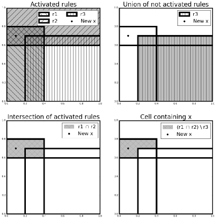
Figure 1: Different steps of the partitioning trick for a set of three hyperrectangles $\{\mathbf{r}_{1},\mathbf{r}_{2},\mathbf{r}_{3}\}$ of $[0,1]^{2}$ and a new observation $\mathbf{x}=(0.1,0.7)$. It is important to notice that the cell containing $\mathbf{x}$, $(\mathbf{r}_{1}\cap\mathbf{r}_{2})\setminus\mathbf{r}_{3}$, is not a hyperrectangle so it does not define a rule.

Proposition 2.1.

Let $\mathcal{S}_{n}$ be a set of $R$ rules selected from a sample $D_{n}$. Then, the complexity to calculate $\mu(K_{n}(\mathbf{x}),D_{n})$ for a new observation $\mathbf{x}\in\mathcal{X}$ is $O(nR)$.

Proof.

It is sufficient to notice that $\mu(K_{n}(\mathbf{x}),D_{n})$ can be express as follows:

$$\mu(K_{n}(\mathbf{x}),D_{n})=\dfrac{\sum\limits_{j=1}^{n}y_{j}k(\mathbf{x},\mathbf{x}_{j},\mathcal{S}_{n})}{\sum\limits_{j=1}^{n}k(\mathbf{x},\mathbf{x}_{j},\mathcal{S}_{n})},$$ (5)

with $k(\mathbf{x},\mathbf{x}_{j},\mathcal{S}_{n})=\prod\limits_{i=1}^{R}\left(\mathbf{1}_{\mathbf{x}\in\mathbf{r}_{i}}\mathbf{1}_{\mathbf{x}_{j}\in\mathbf{r}_{i}}+\mathbf{1}_{\mathbf{x}\notin\mathbf{r}_{i}}\mathbf{1}_{\mathbf{x}_{j}\notin\mathbf{r}_{i}}\right)$.

In (5), the complexity $O(nR)$ appears immediately. $\blacksquare$ ∎

2.2 Independent Suitable Rules

Each dimension of $\mathcal{X}$ is discretized into $m_{n}$ classes such that

$$\dfrac{(m_{n})^{d}}{n}\to 0,\qquad n\to\infty.$$ (6)

To do so empirical quantiles of each variable are considered (when it has more than $m_{n}$ different values). Thus, each class of each variable covers about $100/m_{n}$ percent of the sample. This discretization is the reason why RIPE deals with continuous and ordered discrete variables only.

It is a theoretical condition. However, it indicates that $m_{n}$ must be inversely related to $d$: The higher the dimension of the problem, the smaller the number of modalities. It is a way to avoid overfitting.

We first define two crucial numbers:

Definition 2.1.

Let $\mathbf{r}=\prod_{k=1}^{d}I_{k}$ be a hyperrectangle.

1. The number of activations of $\mathbf{r}$ in the sample $D_{n}$ is

   $$n(\mathbf{r},D_{n}):=\sum\nolimits_{j=1}^{n}\mathbf{1}_{\mathbf{x}_{j}\in\mathbf{r}}.$$ (7)

2. The complexity of $\mathbf{r}$ is

   $$cp(\mathbf{r})=d-\#\{1\leq k\leq d;I_{k}=\mathcal{X}_{k}\},$$ (8)

We are now able to define a suitable rule.

Definition 2.2.

A rule $\mathbf{r}$ is a suitable rule for a sample $D_{n}$ if and only if it satisfies the two following conditions:

1. Coverage condition.

   $$\dfrac{n(\mathbf{r},D_{n})}{n}\leq\frac{1}{\ln(m_{n})},$$ (9)

2. Significance condition.

   $$\left|\mu(\mathbf{r},D_{n})-\mu(\mathcal{X},D_{n})\right|\geq z(\mathbf{r},D_{n}),$$ (10)

   for a chosen function $z$.

The coverage condition (9) ensures that the coverage ratio $n(\mathbf{r},D_{n})/n$ of a rule tends toward $0$ for $n\to\infty$. It is a necessary condition to prove the consistency of the estimator which it is the purpose of a companion paper.

The threshold in the significance condition (10) is to ensure that the local estimators defined on subsets $\mathbf{r}$ is different than the simplest estimator which is the one who is identically equal to $\mu(\mathcal{X},D_{n})$.

RIPE generates rules of complexity $c\geq 2$ by a suitable intersection of rules of complexity $1$ and rule of complexity $c-1$.

Definition 2.3.

Two rules $\mathbf{r}_{i}$ and $\mathbf{r}_{j}$ define a suitable intersection if and only if they satisfy the two following conditions:

1. Intersection condition:

   $$\begin{split}&\mathbf{r}_{i}\cap\mathbf{r}_{j}\neq\emptyset,\\ &n(\mathbf{r}_{i}\cap\mathbf{r}_{j},D_{n})\neq n(\mathbf{r}_{i},D_{n}),\\ &n(\mathbf{r}_{i}\cap\mathbf{r}_{j},D_{n})\neq n(\mathbf{r}_{j},D_{n})\end{split}$$ (11)

2. Complexity condition:

   $$cp(\mathbf{r}_{i}\cap\mathbf{r}_{j})=cp(\mathbf{r}_{i})+cp(\mathbf{r}_{j}).$$ (12)

The intersection condition (11) avoids adding a useless condition for a rule. In other words, to define a suitable intersection $\mathbf{r}_{i}$ and $\mathbf{r}_{j}$ must not be satisfied for the same observations of $D_{n}$. And the complexity condition (12) means that $\mathbf{r}_{i}$ and $\mathbf{r}_{j}$ have no marginal index $k$; $\mathbf{1}_{k}\subsetneq\mathcal{X}_{k}$, in common of $\mathcal{X}$.

3 RIPE Algorithm

We now describe the methodology of RIPE for designing and selecting rules. The Python code is available at https://github.com/VMargot/RIPE.

The main algorithm is described as Algorithm 1. The methodology is divided into two parts. The first part aims at finding all suitable rule and the second one aims at selecting a small subset of suitable rules that estimate accurately the objective $g^{*}$.

The parameters of the algorithm are:

• $m_{n}$, the sharpness of the discretization, which must fulfill (6);

• $\alpha\in[0,1]$, which specifies the false rejecting rate of the test;

• $z$, the significance function of the test;

• and $M\in\mathbb{N}$, the number of rules of complexity $1$ and $c-1$ used to define the rules of complexity $c$.

Global parameters :  $m_{n}$, $\alpha$, $z$ and $M$;

Input:

• $(\mathbf{X},\mathbf{y})\in\mathbb{R}^{n(d+1)}$: data

Output:

• $\mathcal{S}$: the set of selected rules

1 Set ${h}_{n}=1/\ln(m_{n})$ the maximal coverage ratio of a rule;

2 $\tilde{}\mathbf{X}\leftarrow Discretize(\mathbf{X},{m}_{n})$ discretization in $m_{n}$ modalities;

3 $\mathcal{R}\leftarrow Calc\_cp1((\tilde{}\mathbf{X},\mathbf{y}),h_{n})$;

4 for $c=2,\dots,d$ do

5       $\mathcal{R}^{\prime}\leftarrow Calc\_cpc((\tilde{}\mathbf{X},\mathbf{y}),\mathcal{R},c,h_{n})$;

6       if $len(\mathcal{R}^{\prime})=0$ then

7             Break;

8            

9       else

10             $\mathcal{R}\leftarrow append(\mathcal{R},\mathcal{R}^{\prime})$;

11            

12      

13 end for

14$\mathcal{R}\leftarrow Sort\_by\_risk(\mathcal{R},(\tilde{}\mathbf{X},\mathbf{y}))$;

15 $\mathcal{S}\leftarrow Select(\mathcal{R},(\tilde{}\mathbf{X},\mathbf{y}))$;

16 Return $\mathcal{S}$;

Algorithm 1 Main

3.1 Designing Suitable Rules

The design of suitable rules is made recursively on their complexity. It stops at a complexity $c$ if no rule is suitable or if the maximal complexity $c=d$ is achieved.

3.1.1 Complexity $1$:

The first step is to find suitable rules of complexity $1$. This part is described as Algorithm 2. First notice that the complexity of evaluating all rules of complexity $1$ is $O(ndm_{n}^{2})$.

Rules of complexity $1$ are the base of RIPE search heuristic. So all rules are considered and just suitable are kept, i.e rules that satisfied the coverage condition (9) and the significance condition (10). Since rules are considered regardless of each others, the search can be parallelized.

At the end of this step, the set of suitable rules is sorted by their empirical risk (3), $\mathcal{L}_{n}(\hat{g}^{\{\mathbf{r}\}})$, with $\hat{g}^{\{\mathbf{r}\}}$ the predictor based on exactly one rule $\mathbf{r}$.

Global parameters :  $m_{n}$, $\alpha$ and $z$;

Input:

• $(\mathbf{X},\mathbf{y})\in\mathbb{R}^{n(d+1)}$: data

• $h_{n}$: parameter

Output:

• $\mathcal{R}$: the set of all suitable rules of complexity $1$;

1 $\mathcal{R}\leftarrow\emptyset$;

2 for $i=1,\dots,d$ do

3       $\mathbf{x}_{i}\leftarrow\mathbf{X}[i]$, the i^th feature ;

4       for $b_{min}=0,\dots,{m}_{n}$  do

5             for $b_{max}=b_{min},\dots,{m}_{n}$ do

6                   Set $\mathbf{r}=\prod_{k=1}^{d}I_{k}$ with $\begin{cases}I_{k}=[0,m_{n}],\,k\neq i\\ I_{i}=\left[b_{min},b_{max}\right]\\ \end{cases}$;

7                   if is_suitable($\mathbf{r}$, $(\mathbf{X},\mathbf{y})$, $h_{n}$, $z$, $\alpha$) then

8                         $\mathcal{R}\leftarrow append(\mathcal{R},\mathbf{r})$;

9                        

10                  

11             end for

12            

13       end for

14      

15 end for

Return $\mathcal{R}$

Algorithm 2 Calc_cp$1$

3.1.2 Complexity $c$:

Among the suitable rules of complexity $1$ and $c-1$ sorted by their empirical risk (3), RIPE selects the $M$ first rules of each complexity ($1$ and $c-1$). Then it generates rules of complexity $c$ by pairwise suitable intersection according to the definition 2.3. It is easy to see that the complexity of evaluating all rules of complexity $c$ obtained from their intersections is then $O(nM^{2})$.

The parameter $M$ is to control the computing time and it is fixed by the statistician. This part is described as Algorithm 3.

Global parameters :  $\alpha$, $z$ and $M$;

Input:

• $(\mathbf{X},\mathbf{y})\in\mathbb{R}^{n(d+1)}$: data

• $\mathcal{R}$: set of rules of complexity up to $c-1$

• $c$: complexity

• $h_{n}$: parameter

Output:

• $\mathcal{R}_{c}$: set of suitable rules of complexity ${c}$

1 $\mathcal{R}_{c}\leftarrow\emptyset$;

2 $\mathcal{R}\leftarrow Sort\_by\_risk(\mathcal{R},(\mathbf{X},\mathbf{y}))$;

3 $\mathcal{R}_{1}\leftarrow$ the $M$ first rules of complexity $1$ in $\mathcal{R}$;

4 $\mathcal{R}_{c-1}\leftarrow$ the $M$ first rules of complexity ${c}-1$ in $\mathcal{R}$;

5 if $\mathcal{R}_{1}\neq\emptyset$ and $\mathcal{R}_{c-1}\neq\emptyset$ then

6       for $\mathbf{r}_{1}$ in $\mathcal{R}_{1}$ do

7             for $\mathbf{r}_{2}$ in $\mathcal{R}_{c-1}$ do

8                   if is_suitable_intersection($\mathbf{r}_{1}$, $\mathbf{r}_{2}$) then

9                         Set $\mathbf{r}=\mathbf{r}_{1}\cap\mathbf{r}_{2}$;

10                         if is_suitable($\mathbf{r}$, $(\mathbf{X},\mathbf{y})$, $h_{n}$, $z$, $\alpha$) then

11                               $\mathcal{R}_{c}\leftarrow append(\mathcal{R}_{c},\mathbf{r})$;

12                              

13                        

14                  

15             end for

16            

17       end for

18      

Return $\mathcal{R}_{c}$

Algorithm 3 Calc_cp$c$

3.2 Selection of Suitable Rules

After designing suitable rules, RIPE selects an optimal set of rules. Let $\mathcal{R}_{n}$ be the set of all suitable rules generated by RIPE. The optimal subset $\mathcal{S}_{n}^{*}\subset\mathcal{R}_{n}$ is defined by

$$\mathcal{S}_{n}^{*}:=\operatorname*{arg\,min}\limits_{\mathcal{S}\subset\mathcal{R}_{n}}\mathcal{L}_{n}(\hat{g}^{\{\mathcal{S}\}})$$ (13)

is the empirical risk (3) of the predictor based on $\mathcal{S}$.

Each computation of the empirical risk (13) requires the partition from the set $\mathcal{S}$ of rules, as described in Section 2.1. The complexity to solve (13) naively, comparing all the possible sets of rules, is exponential in the number of suitable rules.

To work around this problem, RIPE uses Algorithm 4, a greedy recursive version of the naive algorithm: it does not explore all the subsets of $\mathcal{R}_{n}$. Instead, it starts with a single rule, the one with minimal risk, and iteratively keeps/leaves the rules by comparing the risk of a few combinations of these rules. More precisely, suppose that

• $\mathbf{r}_{1},\dots,\mathbf{r}_{N}$ are the suitable rules, sorted by increasing empirical risk;

• $\mathbf{r}_{1},\dots,\mathbf{r}_{k},\;k<N,$ have already been tested;

• $j$ of them, say $\mathcal{S}\subset\{\mathbf{r}_{1},\dots,\mathbf{r}_{k}\}$ have been kept, the $k-j$ other being left.

Then $\mathbf{r}_{k+1}$ is tested in the following way :

• Compute the risk of $\mathcal{S}$, $\mathcal{S}\cup\{\mathbf{r}_{k+1}\}$ and of all $\mathcal{S}\cup\{\mathbf{r}_{k+1}\}\!\setminus\!\{\mathbf{r}\}$ for $\mathbf{r}\in\mathcal{S}$;

• Keep the rules corresponding to the minimal risk;

• Possibly leave once for all, the rule in $\{\mathbf{r}_{1},\dots,\mathbf{r}_{k+1}\}$ which is not kept at this stage.

Thus, instead of testing the $2^{N}$ subsets of rules, we make $N$ steps and at the $k^{\text{th}}$ step we test at most $k+2$ (and usually much less) subsets, which leads to a theoretical overall maximum of $O(N^{2})$ tested subsets. The heuristic of this strategy is that rules with low risk are more likely to be part of low risk subsets of rules; and the minimal risk is searched in subsets of increasing size.

Input:

• $\mathcal{R}$: set of rules sorted by increasing risk

• $(\mathbf{X},\mathbf{y})\in\mathbb{R}^{n(d+1)}$: data

Output:

• $\mathcal{S}$: subset of selected rules approaching the argmin (13) over all subsets of $\mathcal{R}$ ;

1 Set $\mathcal{S}=\{\mathcal{R}(1)\}$;

2 for $i=2,\dots,len(\mathcal{R})$ do

3       Set $\mathfrak{S}=\{\;\mathcal{S}\;;\;\mathcal{S}\!\cup\!\{\mathcal{R}(i)\}\;\}$;

4       for j=1,…,len($\mathcal{S}$) do

5             $\mathfrak{S}\leftarrow append(\;\mathfrak{S}\;;\;\mathcal{S}\!\cup\!\{\mathcal{R}(i)\}\!\!\setminus\!\!\{\mathcal{S}(j)\}\;)$

6       end for

7      $\mathfrak{S}\leftarrow Sort\_by\_risk(\mathfrak{S},(\mathbf{X},\mathbf{y}))$;

8       $\mathcal{S}\leftarrow\mathfrak{S}(1)$

9 end for

10Return $\mathcal{S}$;

Algorithm 4 Select

4 Experiments

The experiments have been done with Python. To assure reproducibility the random seed has been set at $42$. The codes of these experiments are available in GitHub with the package RIPE.

4.1 Artificial Data

The purpose here it is to understand the process of RIPE, and how it can explain a phenomenon. We generate a dataset of $n=5000$ observations with $d=10$ features. The target variable $Y$ depends on two features $X_{1}$ and $X_{2}$ whose are identically distributed on $[-1,1]$. In order to simulate features assimilated to white noise, the others variables follow a centered- reduced normal distribution $\mathcal{N}(0,1)$. The model is the following

$$y_{i}=F^{*}(\mathbf{x}_{i})+\epsilon_{i}$$ (14)

with $\epsilon_{i}\sim\mathcal{N}(0,1)$ and

$$F^{*}(\mathbf{x}_{i})=-2\times\mathbf{1}_{\left\{x_{1,i}^{2}+x_{2,i}^{2}>0.8\right\}}+2\times\mathbf{1}_{\left\{x_{1,i}^{2}+x_{2,i}^{2}<0.5\right\}}$$ (15)

The dataset is randomly split into training set $D^{1}_{m}$ and test set $D^{2}_{l}$ such as $D^{1}_{m}$ represents $60\%$ of the dataset. RIPE uses significance test based on (17) with a threshold $\alpha=0.05$ and $m_{n}=5$.

On Figure 2, we have on the left, the true model (15) according to $X_{1}$ and $X_{2}$ with the realization of $Y$ not used during the learning. On the right, the model inferred by RIPE.

On Tab 1 we represent the set of selected rules. In this case rules form a covering of the features space. So it is not necessary to add the no rule satisfied statement (see Def 1.6).

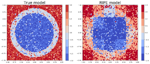
Figure 2: The true model vs the model inferred by RIPE.

Rule	Conditions	Coverage	Prediction	Z	$MSE$
R 0(2)-	$X0\in[1.0,3.0]\ \&\ X1\in[1.0,3.0]$	$0.36$	$-0.91$	$0.09$	$2.14$
R 1(2)-	$X0\in[1.0,3.0]\ \&\ X1\in[2.0,4.0]$	$0.36$	$-0.57$	$0.09$	$3.31$
R 2(2)-	$X0\in[2.0,4.0]\ \&\ X1\in[1.0,3.0]$	$0.35$	$-0.54$	$0.09$	$3.40$
R 3(1)-	$X0\in[2.0,3.0]$	$0.40$	$-0.46$	$0.08$	$3.48$
R 4(1)-	$X0\in[1.0,2.0]$	$0.40$	$-0.43$	$0.08$	$3.55$
R 5(1)-	$X1\in[1.0,2.0]$	$0.40$	$-0.43$	$0.08$	$3.55$
R 6(1)+	$X0=4.0$	$0.20$	$0.63$	$0.11$	$3.65$
R 7(1)+	$X1=4.0$	$0.20$	$0.56$	$0.12$	$3.74$
R 8(1)+	$X1\in[0.0,1.0]$	$0.40$	$0.19$	$0.08$	$3.95$
R 9(1)+	$X0\in[0.0,1.0]$	$0.40$	$0.15$	$0.08$	$3.99$

Table 1: Summary of selected rules with conditions interval express as modalities

4.2 High Dimension Simulation

In this simulation, we use the function make_regression, from the Python package sklearn ([11]), to generate a random linear regression model with $n$ observations and $d$ variables. Among these variables, $p$ are informative and the rest are gaussian centered noise.

In this example we take $n=500$, $d=1000$ and $p=5$ to simulate a noisy high dimensional problem. The data are randomly split into a training set and a test set, with a ratio of $60\%$ \$40\%$, respectively.

We use two others algorithms in this case: Decision Tree (DT) [3] without pruning and Random Forests (RF) [2], all from the package of python sklearn [11]. In order to evaluate the performance of our model, the normalized mean square error ($NMSE$) is computed.

Results are summarized in Tab 3. Difference between the $NMSE$ of the training and the $NMSE$ of test indicates that Decision Tree and Random Forests overfit in this context. Conversely, RIPE infers a model which is more general (see Tab 3). Indeed, RIPE is able to describe the model with only $14$ rules (see Tab 2) which have conditions on only seven variables from $1000$. Among these selected variables only two are very important $X_{976}$ and $X_{298}$ (see Tab 4).

In this case, RIPE discretizes each variable in $5$ modalities from $0$ to $4$. Table 2 presents the selected rules with their conditions. The rule $R14$ is the no rule satisfied statement (see Definition 1.6).

Rule	Conditions	Coverage	Prediction	Z	$MSE$
R 1(2)-	$X_{976}\in[0.0,2.0]\ \&\ X_{298}\in[0.0,2.0]$	$0.35$	$-0.83$	$0.28$	$7808.24$
R 2(1)-	$X_{976}=0.0$	$0.20$	$-1.07$	$0.46$	$8907.38$
R 3(1)+	$X_{976}=4.0$	$0.20$	$0.88$	$0.41$	$10081.34$
R 4(2)-	$X_{976}\in[0.0,1.0]\ \&\ X_{336}\in[0.0,1.0]$	$0.19$	$-0.89$	$0.40$	$10245.30$
R 5(2)+	$X_{298}\in[2.0,4.0]\ \&\ X_{976}\in[2.0,3.0]$	$0.24$	$0.65$	$0.27$	$10781.00$
R 6(1)+	$X_{298}=4.0$	$0.20$	$0.73$	$0.43$	$10813.83$
R 7(1)-	$X_{298}=0.0$	$0.20$	$-0.73$	$0.42$	$10822.09$
R 8(2)-	$X_{298}\in[0.0,1.0]\ \&\ X_{336}\in[0.0,1.0]$	$0.20$	$-0.66$	$0.38$	$11109.50$
R 9(2)+	$X_{976}\in[2.0,4.0]\ \&\ X_{564}=4.0$	$0.14$	$0.77$	$0.45$	$11253.10$
R 10(2)+	$X_{976}\in[2.0,4.0]\ \&\ X_{163}=4.0$	$0.13$	$0.75$	$0.44$	$11419.93$
R 11(2)-	$X_{976}\in[0.0,1.0]\ \&\ X_{945}=2.0$	$0.10$	$-0.87$	$0.51$	$11427.16$
R 12(2)-	$X_{976}\in[0.0,1.0]\ \&\ X_{733}=1.0$	$0.10$	$-0.84$	$0.58$	$11524.60$
R 13(1)+	$X_{976}=3.0$	$0.20$	$0.55$	$0.31$	$11548.05$
R 14	No rule activated	$0.02$	$-0.35$	$0.45$	$12440.40$

Table 2: Summary of selected rules with conditions interval express as modalities

Algorithm	Parameters	$NMSE$ training	$NMSE$ test	Nb of rules	Complexity max
DT	/	$0.0$	$0.46$	$350$	$14$
RF	m_tree = $200$ m_try = $d/3$	$0.04$	$0.39$	$128.25$	$21$
RIPE	$M$=300 z: see (17) $\alpha$=$0.05$	$0.13$	$0.30$	$14$	$2$

Table 3: Performance results of RIPE compared to two supervised learning algorithms: The Decision Tree (DT) and the Random Forests (RF).

Variable	$X_{976}$	$X_{298}$	$X_{336}$	$X_{163}$	$X_{945}$	$X_{565}$	$X_{733}$
Count	$10$	$5$	$2$	$1$	$1$	$1$	$1$

Table 4: Count of variable occurencies in rules selected by RIPE.

4.3 Real Data

In this section, we present a quick overview of the use of the alogirthm RIPE on the well-known Kaggle’s dataset: Titanic. It is a binary classification problem. The goal is to predict which passengers survived the tragedy. We have kept only $7$ features. We have dropped features Name, Ticket Number, and Cabin Number which are considered irrelevant for a first study, and we haven’t done data engineering.

The accuracy rate given by Kaggle for RIPE’s predictions on the test set is $0.765$, but the most interesting output is the description of the model.

This can be sum up in the table 5 and with the two following figures. Figure 3 shows that the most important feature is the fare which appears seven times in the set of selected rules. The figure 4 permits to be more specific. Indeed, we can notice that the cheaper the ticket, the higher the risk to die.

This example shows the kind of interpretation that RIPE could offer to a statistical study on an unknown dataset.

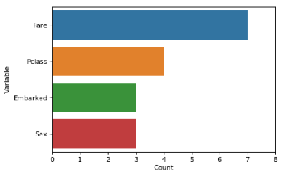
Figure 3: Distribution of rules by variables

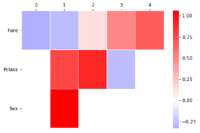
Figure 4: Sum of the prediction of rules for each quantitative variable by modalities

Rule	Conditions	Coverage	Prediction	Z	$MSE$
R 0(2)+	$Sex=female\ \&\ Pclass\in[1.0,2.0]$	$0.19$	$1.16$	$0.26$	$0.32$
R 1(2)+	$Sex=female\ \&\ Fare=4.0$	$0.11$	$1.09$	$0.35$	$0.41$
R 3(2)+	$Sex=female\ \&\ Embarked\in[C,Q]$	$0.12$	$0.93$	$0.32$	$0.42$
R 2(1)+	$Pclass=1.0$	$0.24$	$0.51$	$0.21$	$0.43$
R 5(1)-	$Fare\in[0.0,1.0]$	$0.38$	$-0.38$	$0.14$	$0.43$
R 6(2)+	$Pclass\in[1.0,2.0]\ \&\ Fare=4.0$	$0.18$	$0.63$	$0.25$	$0.43$
R 4(2)-	$Pclass=3.0\ \&\ Fare\in[0.0,2.0]$	$0.47$	$-0.27$	$0.13$	$0.44$
R 7(2)+	$Fare\in[2.0,4.0]\ \&\ Embarked\in[C,NaN]$	$0.15$	$0.54$	$0.27$	$0.45$
R 8(2)+	$Fare\in[2.0,4.0]\ \&\ Embarked\in[C,Q]$	$0.17$	$0.45$	$0.25$	$0.45$
R 9(1)-	$Fare\in[1.0,2.0]$	$0.41$	$-0.16$	$0.14$	$0.46$
R 10	No rule activated	$0.09$	$-0.40$	$0.28$	$0.47$

Table 5: Summary of selected rules with conditions interval express as modalities

5 Conclusion and Future Work

In this paper we present a novel understandable predictive algorithm, named RIPE. Considering the regression function is the best predictor RIPE has been developed to be a simple and accurate estimator of the regression function. The algorithm identified a set of suitable rules, not necessary disjoint, of the form If-Then such as their If conditions are hyperrectangles of the features space $\mathcal{X}$. Then, the estimator is built on the partition generated by the partitioning trick. Its computational complexity is linear in the data dimension $O(dn)$.

RIPE is different from existing methods which are based on a space-partitioning tree. It is able to generate a fine partition from a set of suitable rules, reasonably quickly such that their cells are explained as a list of suitable rules. Whereas there is a one-to-one correspondence between a rule and a cell of a partition provided by a decision tree. So to have a finer partition decision trees must be deeper and rules become less and less understandable. Furthermore, on the contrary to decision trees, the partition generated by RIPE can have cells which are not hyperrectangles.

A paper on the universal consistency of RIPE under some technical conditions is in preparation.

Appendix: Examples of Significance Function

Here, we present three functions $z$ used in practice.

1. The first one is based on the Hœffding’s inequality [8]:

   $$z(\mathbf{r},D_{n},\alpha)=\dfrac{(M-m)\sqrt{\ln(2/\alpha)}}{\sqrt{2n(\mathbf{r},D_{n})}},$$ (16)

   where $M=\max\limits_{i\in\{1,\dots,n\}}y_{i}$ and $m=\min\limits_{i\in\{1,\dots,n\}}y_{i}$.

2. The second one is based on the Bernstein’s inequality:

   $$z(\mathbf{r},D_{n},\alpha)=\dfrac{1}{6n(\mathbf{r},D_{n})}\left(M\ln\left(\dfrac{2}{\alpha}\right)+\sqrt{M^{2}\ln\left(\dfrac{2}{\alpha}\right)^{2}+72v\ln\left(\dfrac{2}{\alpha}\right)}\right),$$ (17)

   where $M=\max\limits_{i\in\{1,\dots,n\}}y_{i}$ and $v=\sum_{i=1}^{n}y_{i}^{2}$.

3. And the last one is

   $$z(\mathbf{r},D_{n})\>=\sqrt{\left(\beta_{\mathbf{r},n}\dfrac{1}{n-1}\sum_{i=1}^{n}\left(Y_{i}-\bar{Y}\right)^{2}-\dfrac{1}{n(\mathbf{r},D_{n})-1}\sum_{i=1}^{n}\mathbf{1}_{X_{i}\in\mathbf{r}}\left(Y_{i}-\bar{Y}_{\mathbf{r}}\right)^{2}\right)},$$ (18)

   where

   $$\beta_{\mathbf{r},n}=\dfrac{n}{\sum_{\mathbf{r}^{\prime}\in\mathcal{S}_{n}}n(\mathbf{r}^{\prime},D_{n})}\max\limits_{A}\#\{\mathbf{r}^{\prime}\in\mathcal{S}_{n}:\mathbf{r}^{\prime}\cap A\neq\emptyset\},$$ (19)

   with the $\max$ is taken upon the set of cells of $\mathcal{K}(\mathcal{S}_{n})$ contained in $\mathbf{r}$. It means the set defined by

   $$\left\{A\in\mathcal{K}(\mathcal{S}_{n}):A\subseteq\mathbf{r}\right\}.$$

References

- [1] S. Arlot and A. Celisse. A survey of cross-validation procedures for model selection. Statistics Surveys, 4:40–79, 2010. Published in Statistics Surveys.
- [2] L. Breiman. Random forests. Machine learning, 45(1):5–32, 2001.
- [3] L. Breiman, J. Friedman, R. Olshen, and C. Stone. Classification and Regression Trees. CRC press, 1984.
- [4] H.A. Chipman, E.I. George, and R.E. McCulloch. Bayesian cart model search. Journal of the American Statistical Association, 93(443):935–948, 1998.
- [5] K. Dembczyński, W. Kotłowski, and R. Słowiński. Solving regression by learning an ensemble of decision rules. In International Conference on Artificial Intelligence and Soft Computing, pages 533–544. Springer, 2008.
- [6] J.H. Friedman and B.E. Popescu. Predective learning via rule ensembles. The Annals of Applied Statistics, pages 916–954, 2008.
- [7] L. Györfi, M. Kohler, A. Krzyzak, and H Walk. A Distribution-Free Theory of Nonparametric Regression. Springer Science & Business Media, 2006.
- [8] W Hoeffding. Probability inequalities for sums of bounded random variables. Journal of the American statistical association, 58(301):13–30, 1963.
- [9] Laurent Hyafil and Ronald L Rivest. Constructing optimal binary decision trees is np-complete. Information processing letters, 5(1):15–17, 1976.
- [10] B. Letham, C. Rudin, T.H. McCormick, and D. Madigan. Interpretable classifiers using rules and bayesian analysis: Building a better stroke prediction model. The Annals of Applied Statistics, 9(3):1350–1371, 2015.
- [11] F. Pedregosa, G. Varoquaux, A. Gramfort, V. Michel, B. Thirion, O. Grisel, M. Blondel, P. Prettenhofer, R. Weiss, V. Dubourg, J. Vanderplas, A. Passos, D. Cournapeau, M. Brucher, M. Perrot, and E. Duchesnay. Scikit-learn: Machine learning in Python. Journal of Machine Learning Research, 12:2825–2830, 2011.
- [12] J. R Quinlan. C4.5: Programs for Machine Learning. Morgan Kaufmann Publishers Inc., San Francisco, CA, USA, 1993.
- [13] H. Yang, C. Rudin, and M. Seltzer. Scalable bayesian rule lists. In Proceedings of the 34th International Conference of Machine Learning (ICML’17), 2017.