Shack-Hartmann wavefront sensor sensitivity loss factor estimation in partial correction regime

Abstract

In typical adaptive optics applications, the atmospheric residual turbulence affects the wavefront sensor response decreasing its sensitivity. On the other hand, wavefront sensors are generally calibrated in diffraction limited condition, and, so, the interaction matrix sensitivity may differ from the closed loop one. The ratio between the two sensitivities, that we will call the sensitivity loss factor, has to be estimated to retrieve a well-calibrated measurement. The spots size measurement could give a good estimation, but it is limited to systems with spots well sampled and uniform across the pupil. We present an algorithm to estimate the sensitivity loss factor from closed loop data, based on the known parameters of the closed loop transfer functions. Here we preferred for simplicity the Shack-Hartmann WFS, but the algorithm we propose can be extended to other WFSs.

1 Introduction

In this article we focus on the sensitivity gain of the Wavefront Sensor (WFS), that is the ratio between the calibrated sensitivity and the one obtained during operation. For many applications we need the actual WFS sensitivity to get the correct measurement (very important in open-loop), to proper optimize the temporal controller, and to proper compensate for Non Common Path Aberrations (NCPA). A change on the WFS sensitivity can be caused by a variation of the spot size[1] (strong effect in a quadcell SH) or a change of dark current and/or sky background. In some cases these effects can be measured and so the sensitivity loss factor can be estimated [2, 3, 4], otherwise a specific algorithm should be used to estimate this [5, 6].

In this paper we present an approach to the estimation of this coefficient based on the closed loop Transfer Function (TF) and on the loop data Power Spectral Densities (PSD).

2 Closed Loop Transfer Functions and WFS sensitivity

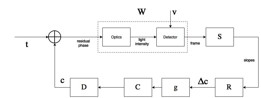
Figure 1: Scheme of a SCAO closed loop system.

Let us consider a Single Conjugate Adaptive Optics (SCAO) closed loop system as the one shown in Figure 1. Note that we choose a SCAO system for simplicity, however other systems, like multi-conjugate adaptive optics[7, 8] MCAO, can also be considered as well. The command vector $c$, and the incremental command vector $\Delta c$ are defined as:

$$c=\frac{gH}{1+gH}t+\frac{gSRCD}{1+gH}v\,,$$ (1)

$$\Delta c=\frac{WSR}{1+gH}t+\frac{SR}{1+gH}v\,,$$ (2)

where:

$$H=WSRCD\,,$$ (3)

$W$ is the WFS (optics + detector), $S$ is the slope computer, $R$ is the reconstruction matrix, $D$ is the deformable mirror, $g$ is the integrator gain vector, $C$ is the controller, $t$ is the turbulence and $v$ the measurement noise vector.
Note that the Rejection Transfer Function (RTF) $H_{R}=\frac{1}{1+gH}$, and the Noise Transfer Function (NTF) $H_{N}=\frac{gH}{1+gH}$ are implicitly present in Equations 1 and 2.

Then, we add an unknown linear coefficient in the WFS Transfer Function (TF), $\alpha$, that will be called sensitivity loss factor. Let us define $W=\alpha W^{\prime}$, so the previous equations become:

$$H=\alpha W^{\prime}SRCD=\alpha H^{\prime}\,,$$ (4)

$$c=\frac{g\alpha H^{\prime}}{1+g\alpha H^{\prime}}t+\frac{gSRCD}{1+g\alpha H^{\prime}}v\,.$$ (5)

$$\Delta c=\frac{\alpha W^{\prime}SR}{1+g\alpha H^{\prime}}t+\frac{SR}{1+g\alpha H^{\prime}}v\,,$$ (6)

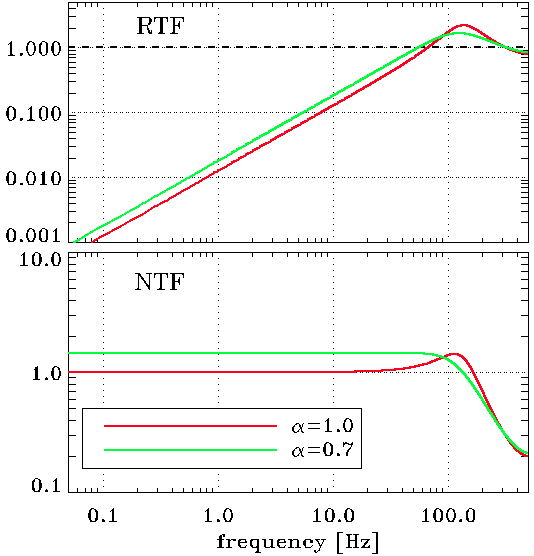
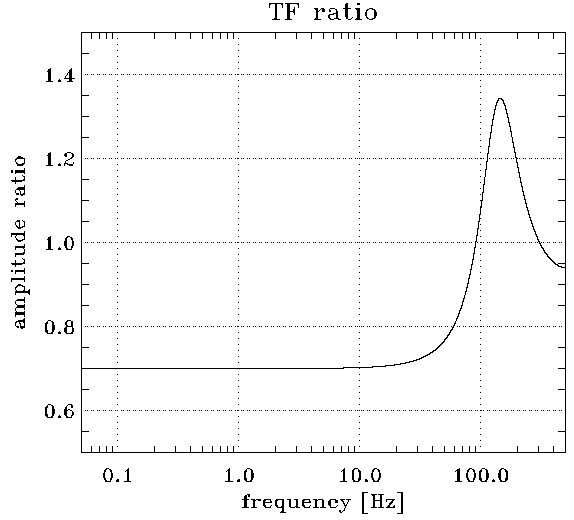
Figure 2: Left: RTFs and NTFs of an AO system with a sampling frequency of 1000Hz, 2 frames of delay, an integrator gain of 0.5 and different WFS sensitivity loss factors (1 and 0.7). Right: Ratio between RTFs (or NTFs) shown on the left.

We set $S=1$, $R=1$, that means they have no dynamics, $W^{\prime}=D=z^{-1}$, that is a pure one step delay dynamics (for a total of two steps of delay), and $C=\frac{1}{1-z^{-1}}$, that is a pure integrator, equations 6 and 5 become:

$$c=\frac{g\alpha}{z^{2}-z+g\alpha}t+\frac{gz}{z^{2}-z+g\alpha}v\,.$$ (7)

$$\Delta c=\frac{\alpha(z-1)}{z^{2}-z+g\alpha}t+\frac{z(z-1)}{z^{2}-z+g\alpha}v\,$$ (8)

The effect of the sensitivity loss factor on RTF and NTF is shown in Figure 2, and on command and incremental command in Figure 3.

Note that it is possible to estimate the RTF, as show in Dessenne et al. [9], but, unfortunately, this estimation is not affected by the sensitivity loss factor: in fact, if we compute this TF using Equations 5 and 6, and $z^{-k}=W^{\prime}$, that is the delay to be added to the commands to be synchronized with the incremental commands, we get:

$$\frac{\Delta c}{\Delta c+cz^{-k}}=\frac{1}{1+gCDz^{-k}}\,,$$ (9)

and so, $\alpha$ has been reduced in the computation.

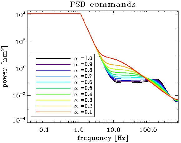
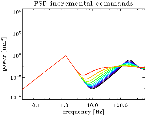
Figure 3: Effects of the sensitivity loss factor $\alpha$. Left: Effect on Tilt command. Right: Effect on Tilt incremental command. Turbulence $r_{0}$ is 0.15m, measurement noise variance is 60nm², integrator gain is 0.7 and total delay is 2 frames.

3 Sensitivity estimation

The sensitivity loss factor, $\alpha$, estimation is evaluated minimizing the cost function in the frequency range $\left[\omega_{1},\omega_{2}\right]$:

$$J(\alpha)=\sum_{\omega=\omega_{1}}^{\omega_{2}}{(\mathrm{PSD}\{\Delta c(\omega)\}-\hat{K}(\omega,\alpha))^{2}}\,,$$ (10)

where:

$$\begin{multlined}\hat{K}(\omega,\alpha)=\left(\frac{\alpha W^{\prime}SR}{1+g\alpha H^{\prime}}\right)^{2}\mathrm{PSD}\{t(\omega)\}+\\ \left(\frac{SR}{1+g\alpha H^{\prime}}\right)^{2}\mathrm{PSD}\{v(\omega)\}\,,\end{multlined}\hat{K}(\omega,\alpha)=\left(\frac{\alpha W^{\prime}SR}{1+g\alpha H^{\prime}}\right)^{2}\mathrm{PSD}\{t(\omega)\}+\\ \left(\frac{SR}{1+g\alpha H^{\prime}}\right)^{2}\mathrm{PSD}\{v(\omega)\}\,,$$ (11)

and the operator:

$$\mathrm{PSD}\{x(\omega)\}\triangleq\langle|x(\omega)|^{2}\rangle$$ (12)

denotes the temporal Power Spectral Density (PSD) of $x$.
So, summarizing, we search for the sensitivity loss factor, $\alpha$, which minimizes the difference between the incremental command PSD and the PSD, computed filtering the inputs PSDs by the $\alpha$ dependent TFs.
Note that here we suppose to know exactly both the turbulence $t$ and the measurement noise $v$. In a real system these data should be estimated before running the sensitivity loss factor estimation.

4 Examples

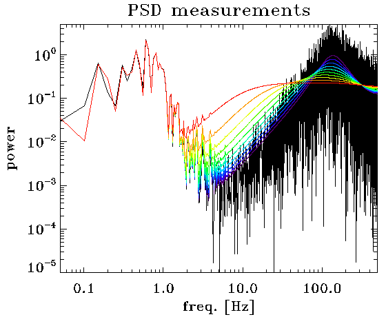
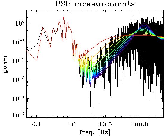
Figure 4: Effects of a spot size on the closed loop measurement PSD. Left: spot size as in calibration. Right: bigger spot size (spot convoled with gaussian with a FWHM of 8 pixels, corresponding to 1,84arcsec). Input Tip-Tilt RMS is 255nm, measurement noise variance is 10nm², integrator gain is 0.5 and total delay is 2 frames. $\alpha=1$ means no sensitivity gain change.

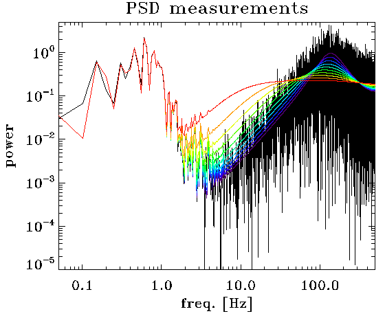
Figure 5: Effects of a strong background on the closed loop measurement PSD. Left: no background as in calibration. Right: 100ph/pixel/frame background (sub-aperture collects 40000ph/frame from the guide star). Input Tip-Tilt RMS is 255nm, measurement noise variance is 10nm², integrator gain is 0.5 and total delay is 2 frames.

In this section we present two examples, showing the effect of a spot size change on sensitivity for a quad-cell SH WFS and the effect of a background variation on a Center of Gravity (CoG) SH WFS. For both examples, we run a numerical simulation of a simple system, with a single sub-aperture SH and with a phase containing only tip-tilt, using the PASSATA software[10].
The parameters of the simulations are:

• WFS FoV = 2.5arcsec;

• dimension of the sub-aperture (side) = 0.2m;

• number of pixels of the detector (side) = 12;

• WFS central wavelength = 750nm;

• input Tip-Tilt RMS = 255nm.

In the first example we run the same simulation for two spot sizes: in the first case with the Diffraction Limited (DL) spot (FWHM=0.77arcsec) and the second case we convolve the DL spot with a 2D Gaussian shape with FWHM of 8 pixels (FWHM=1.84arcsec). In both cases we use the quad-cell algorithm to compute the slopes. We know from calibration that the slope coefficient is 0.0080nm^-1 for a DL spot and 0.0028nm^-1 for a DL spot convolved with the 2D Gaussian shape with FWHM of 8 pixels, hence, the relative sensitivity should be 0.35 (almost the ratio between the two spots size: 0.77/1.84). The frequency range, $\left[\omega_{1},\omega_{2}\right]$, chosen is $[50,500]$. In Figure 4 the measurement PSD for the two cases are shown. The estimated sensitivity loss factor of the first case is, as expected, 1 and for the second case is about 0.35 (between the yellow and the green lines).
As for the first example in the second one we run the same simulation twice: the first time with no background and the second time we add a background of 100ph/pixel/frame (sub-aperture collects 40000ph/frame from the guide star). In both cases we use the CoG algorithm to compute the slopes. Sky background photons increase the denominator of the slope computation of a factor 0.36 ($\frac{14400}{40000}$) and so the gain should be 0.74 ($\frac{1}{1+0.36}$). The frequency range, $\left[\omega_{1},\omega_{2}\right]$, chosen is again $[50,500]$. In Figure 5 the measurement PSD for the two cases are shown. The estimated sensitivity loss factor of the first case is, as expected, 1 and for second case is about 0.75 (between light blue and blue-green lines).
With these two examples we saw how spot size and background noise affect the sensitivity and how the sensitivity gain translates on modification of the TF, producing measurable effects on the PSD. Actually, we estimate the sensitivity gain, $\alpha$, analysing the PSD.

5 Conclusions

An accurate estimate of the WFS sensitivity is essential to get the correct measurement amplitude in the AO loop. We show in this paper how the WFS sensitivity affects the transfer functions of the closed loop, producing measurable effects on the closed loop and inputs data PSDs, so that PSD analysis can be used to estimate the sensitivity gain. The main limitation of this work is that, in most cases, a direct measurements of the input data is not available. This is the reason why further work is needed to find a method to estimate the WFS sensitivity when only closed loop data is available.

On the other hand, a robustness check of the evaluation of the sensitivity gain with respect to the knowledge of the turbulence and with respect to WFS noise estimated, may provide information about the operative range of the method described herein.

References

- [1] Thomas, S. J., Adkins, S., Gavel, D., Fusco, T., and Michau, V., “Study of optimal wavefront sensing with elongated laser guide stars,” MNRAS 387, 173–187 (June 2008).
- [2] Fugate, R. Q., Spinhirne, J. M., Moroney, J. F., Cleis, R. A., Oliker, M. D., Boeke, B. R., Ellerbroek, B. L., Higgins, C. H., Ruane, R. E., Swindle, D. W., Jelonek, M. P., Lange, W. J., Slavin, A. C., Wild, W. J., Winker, D. M., and Wynia, J. M., “Two generations of laser-guide-star adaptive-optics experiments at the starfire optical range,” J. Opt. Soc. Am. A 11, 310–324 (Jan 1994).
- [3] Shelton, J. C., Schneider, T. G., McKenna, D. L., and Baliunas, S. L., “First tests of the cassegrain adaptive optics system of the mount wilson 100-in telescope,” 2534, 72–77 (1995).
- [4] Acton, D. S., Wizinowich, P. L., Stomski, Jr., P. J., Shelton, J. C., Lai, O., and Brase, J. M., “Laboratory calibration of the w.m. keck observatory adaptive optics facility,” Proc. SPIE 3353, 125–131 (1998).
- [5] Véran, J.-P. and Herriot, G., “Centroid gain compensation in shack–hartmann adaptive optics systems with natural or laser guide star,” J. Opt. Soc. Am. A 17, 1430–1439 (Aug 2000).
- [6] Esposito, S., Puglisi, A., Pinna, A., Agapito, G., Veran, J., and Herriot, G., “Non common path aberration correction with non linear WFSs,” in [Adaptive Optics for Extremely Large Telescopes 4 - Conference Proceedings ], (2002).
- [7] Beckers, J. M., “Increasing the size of the isoplanatic patch with multiconjugate adaptive optics.,” in [ESO Conference on Very Large Telescopes and their Instrumentation ], 2, 693–703 (1988).
- [8] Beckers, J. M., “Detailed compensation of atmospheric seeing using multiconjugate adaptive optics.,” in [Active Telescope Systems ], Proc. SPIE 1114, 215–217 (1989).
- [9] Dessenne, C., Madec, P.-Y., and Rousset, G., “Optimization of a Predictive Controller for Closed-Loop Adaptive Optics,” Appl. Opt. 37, 4623–4633 (July 1998).
- [10] Agapito, G., Puglisi, A., and Esposito, S., “Passata: object oriented numerical simulation software for adaptive optics,” Proc. SPIE 9909, 99097E–99097E–9 (2016).