Prescribing the Postsingular Dynamics of Meromorphic Functions

Abstract.

We show that any dynamics on any discrete planar sequence $S$ can be realized by the postsingular dynamics of some transcendental meromorphic function, provided we allow for small perturbations of $S$. This work is motivated by an analogous result of DeMarco, Koch and McMullen in [5] for finite $S$ in the rational setting. The proof contains a method for constructing meromorphic functions with good control over both the postsingular set of $f$ and the geometry of $f$, using the Folding Theorem of [2] and a classical fixpoint theorem [18].

1. Introduction

The singular set $S(f)$ of a meromorphic function $f:\mathbb{C}\rightarrow\hat{\mathbb{C}}$ is the collection of values $w$ at which one can not define all branches of the inverse $f^{-1}$ in any neighborhood of $w$. If $f$ is rational, then $S(f)$ coincides with the collection of critical values of $f$. If $f$ is transcendental meromorphic, $f^{-1}$ may also fail to be defined in a neighborhood of an asymptotic value. The value $w$ is an asymptotic value of $f$ if there is a curve $\gamma(t)\rightarrow\infty$ for which $f(\gamma(t))\rightarrow w$; for instance the exponential map has one asymptotic value at $0$. In the transcendental setting, the set $S(f)$ coincides with the closure of the collection of critical and asymptotic values.

The postsingular set $P(f)$ of a meromorphic function is the closure of the union of forward iterates of the singular set: $\overline{\cup_{n=0}^{\infty}f^{n}(S(f))}$. The singular and postsingular sets play an important rule in the study of the dynamics of $f$, both in the rational and transcendental settings (see for instance [4] for the rational setting, and [17] for the transcendental setting.) The present work addresses the question of allowable geometries and dynamics for the postsingular sets of meromorphic functions. Our main result states that any postsingular dynamics on any discrete sequence can be realized provided one allows for arbitrarily small perturbations of that sequence:

Theorem 1.1.

Let $S\subset\mathbb{C}$ be a discrete sequence (no finite accumulation points) with $4\leq|S|\leq\infty$, let $h:S\rightarrow S$ be any map, and let $\varepsilon>0$. Then there exists a transcendental meromorphic function $f:\mathbb{C}\rightarrow\widehat{\mathbb{C}}$ and a bijection $\psi:S\rightarrow P(f)$ with $|\psi(s)-s|\rightarrow 0$ as $s\rightarrow\infty$, $|\psi(s)-s|\leq\varepsilon$ for all $s\in S$, and $f|_{P(f)}=\psi\circ h\circ\psi^{-1}$.

Theorem 1.1 was inspired by Theorem 1.3 of [5]:

Theorem 1.2.

Let $h:S\rightarrow S$ be an arbitrary map defined on a finite set $S\subset\hat{\mathbb{C}}$ with $|S|\geq 3$. Then there exists a sequence of rigid postcritically finite rational maps $f_{n}$ such that $|P(f_{n})|=|S|$, $P(f_{n})\rightarrow S$ and $f_{n}|P(f_{n})\rightarrow h|S$ as $n\rightarrow\infty$.

The proof of this result in [5] uses iteration on Teichmüller space, whereas the proof of Theorem 1.1 uses a fixpoint theorem [18] and quasiconformal folding methods developed in [2] which we will discuss at length in Section 2. Quasiconformal folding is a method of associating entire functions to certain infinite planar graphs introduced in [2], and was applied there to construct various new examples, such as a wandering domain for an entire function in the Eremenko-Lyubich class. Other applications have been given by Fagella, Godillon and Jarque [9], Fagella, Jarque and Lazebnik [6], Lazebnik [11], [12], Osborne and Sixsmith [14], and Rempe-Gillen [16]. We will review the basic folding construction in Section 2.

We now briefly sketch the proof of Theorem 1.1, leaving details and some special considerations to subsequent sections. We refer to Figure 1. Recall we are given a discrete sequence $S=(s_{n})$ and a map $h:S\rightarrow S$. We construct an infinite graph $G$ by enclosing points $s_{i}\in S$ by disjoint Euclidean discs $D_{i}$ centered at $s_{i}$. As discussed in Sections 3 and 4, we will associate a quasiregular function $g:\mathbb{C}\rightarrow\widehat{\mathbb{C}}$ to the graph $G$. For now, we give the definition of $g$ in a disc $D_{i}$ under the assumption that $h(s_{i})=s_{j}\in\mathbb{D}$. If $z\in D_{i}$, then $g(z):=\rho_{i}\circ(z\mapsto z^{d})\circ\tau_{i}(z)$, where $d\in 2\mathbb{N}$, $\tau_{i}:D_{i}\rightarrow\mathbb{D}$ is a Euclidean similarity (so $\tau_{i}(s_{i})=0$), and $\rho_{i}$ is a quasiconformal self-map of $\mathbb{D}$ which is conformal in $(3/4)\mathbb{D}$ and $\rho|_{\partial\mathbb{D}}=\textrm{id}$. The resulting quasiregular map $g$ will have a critical value at $\rho_{i}(0)$ coming from the critical point $s_{i}$ in $D_{i}$, and we will denote this critical value by $s_{j}^{*}$. The critical value $s_{j}^{*}$ should be thought of as a complex parameter in a small neighborhood of $s_{j}$ for now, and $s_{j}^{*}$ will eventually correspond to $\psi(s_{j})$ where $\psi:S\rightarrow P(f)$ is the bijection of Theorem 1.1. We note that the definition of $g$ on $\mathbb{C}\setminus D_{i}$ will not depend on a choice of $s_{j}^{*}$.

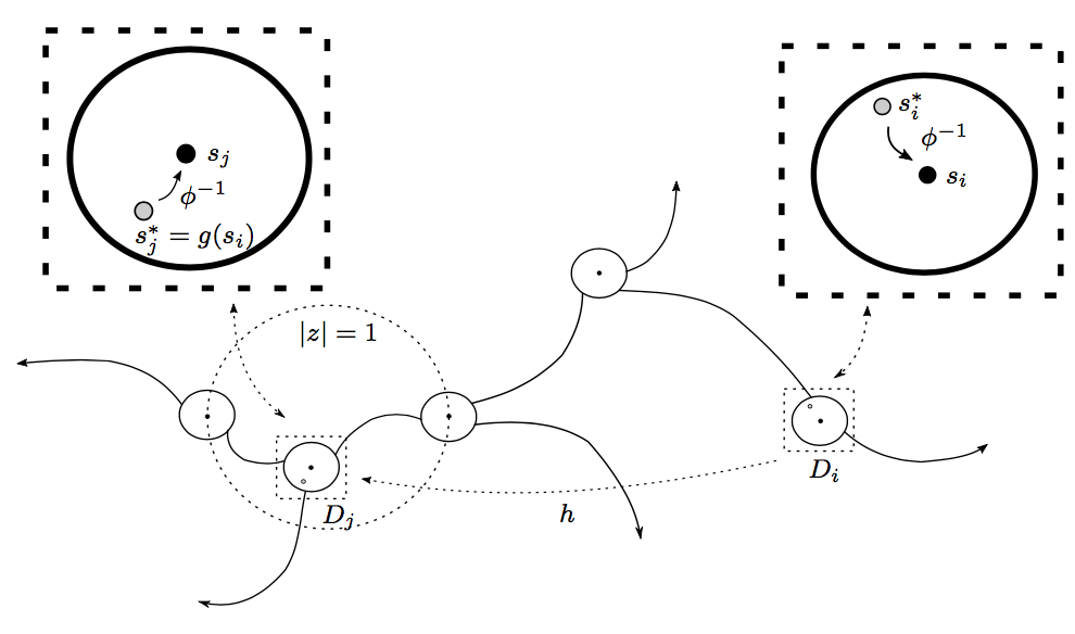
Figure 1. Illustrated is the general strategy in the proof of Theorem 1.1. One applies the Folding Theorem to a graph $G$. Here $s_{i}\in S$ is the center of $D_{i}$, and $s_{i}^{*}$ is a critical value of $g$. The critical point $s_{i}$ of $g$ is sent to a critical value $s_{j}^{*}$ near $s_{j}=h(s_{i})$. One then arranges (using a fixpoint theorem) for $s_{j}^{*}$ to be chosen so that $\phi^{-1}(s_{j}^{*})=s_{j}$.

Next we apply the measurable Riemann mapping theorem to obtain a quasiconformal map $\phi$ so that $g\circ\phi^{-1}$ is holomorphic. The crux of the proof of Theorem 1.1 is to arrange for $s_{j}^{*}$ to be chosen so that $\phi^{-1}(s_{j}^{*})=s_{j}\in S$, over all $j$. Indeed, then for $f=g\circ\phi^{-1}$ we would have $f(S(f))\subset S(f)$ with the desired dynamics, since $g\circ\phi^{-1}(s_{j}^{*})=g(s_{j})=(h(s_{j}))^{*}$ whence again one would have $\phi^{-1}((h(s_{j}))^{*})=h(s_{j})$.

How do we arrange for the parameters $(s_{j}^{*})$ to be chosen so that $\phi^{-1}(s_{j}^{*})=s_{j}$ over all $j$? Let us consider for now the simpler problem of arranging for $\phi^{-1}(s_{j}^{*})=s_{j}$ for some fixed, single index $j$. Of course the Beltrami coefficient $\mu_{g}$ of $g$, and hence the map $\phi$, depends on a choice of $s_{j}^{*}$; indeed varying the critical value $s_{j}^{*}$ varies the dilatation of $\rho_{i}$ in $\mathbb{D}$ (and hence the dilatation of $g$ in a small neighborhood of $\partial D_{i}$). However, as explained in Sections 3 and 4, one can arrange for the (uniformly bounded) dilatation of $g$ to be supported on a neighborhood of $G$ of arbitrarily small area. Hence one may prove that $\phi$ is uniformly close to the identity regardless of our choice of $s_{j}^{*}$ in a small neighborhood of $s_{j}$, say $|\phi(z)-z|<\varepsilon$ over all $z\in\mathbb{C}$.

Now consider moving the parameter $s_{j}^{*}$ continuously in $\overline{D(\varepsilon,s_{j})}$. Namely, for each choice of $w\in\overline{D(\varepsilon,s_{j})}$, we set $s_{j}^{*}:=w$, and we have some resulting quasiregular map $g_{w}$ and correction map $\phi_{w}$ where we have arranged for $|\phi_{w}(z)-z|<\varepsilon$ for $z\in\mathbb{C}$, and $\varepsilon$ is independent of $w$. Thus the map $w\rightarrow\phi_{w}(s_{j})$ is a self-map of $\overline{D(\varepsilon,s_{j})}$, and by continuous dependence on parameters (see Theorem 1.4), $w\rightarrow\phi_{w}(s_{j})$ is continuous. Thus we can apply a fixpoint theorem (in this instance the classical Brouwer fixpoint theorem) to yield some $w_{0}\in\overline{D(\varepsilon,s_{j})}$ so that by choosing $s_{j}^{*}:=w_{0}$, we have $\phi_{w_{0}}^{-1}(s_{j}^{*})=s_{j}$ as needed.

The argument to arrange for the parameters $(s_{j}^{*})$ to be chosen so that $\phi^{-1}(s_{j}^{*})=s_{j}$ over all indices $j$ is similar, however one looks for a fixpoint among a continuous self-mapping of an infinite product of discs centered at the points $s_{j}$, and one appeals to the following infinite-dimensional fixpoint theorem due to Tychonoff [18]:

Theorem 1.3.

Let $V$ be a locally convex topological vector space. For any non-empty compact convex set $X$ in $V$, any continuous function $f:X\rightarrow X$ has a fixpoint.

For us the locally convex topological vector space of Theorem 1.3 will be $\mathbb{C}^{\mathbb{N}}$ (a countable product of complex planes with seminorms $\rho_{i}((z_{j})_{j=1}^{\infty}):=|z_{i}|$), and the non-empty compact convex set $X$ will be an infinite product of closed discs containing the points $s_{i}$ (which is compact by another result of Tychonoff). We remark that a similar fixpoint argument to the one described above was developed independently in [7]. We also record here a statement of continuous dependence on parameters (see, for instance, Theorem 7.5 of [4]):

Theorem 1.4.

(Continuous dependence on parameters) Let $\mu\in L^{\infty}(\mathbb{C})$ with $||\mu||_{L^{\infty}(\mathbb{C})}<1$. Denote by $\phi_{\mu}$ the unique quasiconformal solution of $\frac{\partial\phi_{\mu}}{\partial\bar{z}}=\mu\frac{\partial\phi_{\mu}}{\partial z}$ satisfying some fixed normalization. If $\mu_{n}\rightarrow\mu$ a.e., then $\phi_{\mu_{n}}\rightarrow\phi_{\mu}$ uniformly on compact subsets. Consequently, for any fixed $z\in\mathbb{C}$, the map $L^{\infty}(\mathbb{C})\rightarrow\mathbb{C}$ given by $\mu\rightarrow\phi_{\mu}(z)$ is continuous.

We remark that in the present work we will only need to consider a subclass of Beltrami coefficients $\mu$ which satisfy a strong thinness condition near $\infty$, so that $\phi_{\mu}$ is asymptotically conformal at $\infty$ (see Section 3). For such maps one may normalize $\phi_{\mu}$ such that $\phi_{\mu}(z)=z+O(1/|z|)$ as $z\rightarrow\infty$, and this is the normalization we will always use in the present work.

We leave open the following question arising naturally from the statement of Theorem 1.1, which asks whether it is necessary, in general, to consider perturbations of the sequence $S$:

Question.

Given any discrete planar sequence $S$ and some map $h:S\rightarrow S$, does there always exist a meromorphic $f$ so that $P(f)=S$, and $f|_{S}=h$?

A similar question was asked for finite $S$ and rational $f$ in [5] (see Question 1.2 of [5]):

Question.

Let $S\subset P^{1}(\overline{\mathbb{Q}})$ be a finite set. Is every map $h:S\rightarrow S$ realized by a rigid rational map $f:P(f)\rightarrow P(f)$ with $P(f)=S$?

We also remark that an analogous version of Theorem 1.1 holds for any infinite sequence in $\widehat{\mathbb{C}}$ with a unique accumulation point (not necessarily at $\infty$); in this case the $f$ produced in Theorem 1.1 would have one essential singularity at this accumulation point (not necessarily $\infty$). Thus Theorem 1.1 could be viewed as a statement that Theorem 1.2 of [5] remains true for infinite sets $S$ with a unique accumulation point, provided one is allowed to place an essential singularity of the function $f$ at that accumulation point. It seems plausible, moreover, that any dynamics on a sequence $S$ with $n$ accumulation points could be realized by the postsingular dynamics of a meromorphic function with $n$ essential singularities (one at each accumulation point), provided one allows for perturbations of $S$ as in Theorem 1.1. There are further generalizations to be made in this direction.

Acknowledgements

The authors would like to thank the anonymous referees for their suggestions which led to an improved version of the paper.

2. Bounded geometry graphs

In this and the next section we review the quasiconformal folding method of [2] for constructing entire functions and adapt it to producing meromorphic functions.

Suppose $G$ is an unbounded, locally finite, connected planar graph. We say $G$ has bounded geometry if

1. The edges of $G$ are $C^{2}$ with uniform bounds.

2. The union of edges meeting at a vertex $v$ are a $K$-bi-Lipschitz image of a “star” $\{z\in{\mathbb{C}}:0\leq z^{k}\leq r\}$ for some uniformly bounded $k,K$ ($r$ can be any positive, finite value; the star consists of $k$ equal length segments meeting at evenly spaced angles).

3. For any pair of non-adjacent edges $e$ and $f$, $\text{diam}(e)/\text{dist}(e,f)$ is uniformly bounded from above.

The values for which these conditions hold are called the “bounded geometry constants” of $G$. We define a neighborhood $T_{\gamma}(r)$ of an arc $\gamma$ by

$$T_{\gamma}(r)=\{z\in\mathbb{C}:{\rm{dist}}(z,e)<r\cdot{\rm{diam}}(\gamma)\},$$

and we define a neighborhood $T(r)$ of $G$ by taking the union of these neighborhoods where $\gamma$ ranges over the edges of $G$. This is a sort of Hausdorff neighborhood of $G$, but adapted to the local geometry of $G$ (the “thickness” of the neighborhood is proportional to the diameters of nearby edges).

It is sometimes helpful to replace condition (1) by a stronger condition that was introduced in [3]: we say an arc $\gamma$ is $\varepsilon$-analytic if there is a conformal map on $T_{\gamma}(\varepsilon)$ that maps $\gamma$ to a line segment. We say $G$ is uniformly analytic if it has bounded geometry and every edge is $\varepsilon$-analytic for some fixed $\varepsilon>0$. Note that if we add extra vertices to the edges of a uniformly analytic graph $G$ so as to form a new bounded geometry tree, the new tree is also uniformly analytic with the same constant. All the graphs constructed in this paper will be uniformly analytic.

Since $G$ is connected, the connected components of $\Omega:={\mathbb{C}}\setminus G=\cup_{j}\Omega_{j}$ are simply connected. We further assume that any bounded components are disks and the vertices of $G$ are evenly spaced on the boundary of each disk. We call these the D-components (for “disk components”). To apply the Folding Theorem, D-components need only be bounded Jordan domains, but the special case of disks is all that we need here, and this extra assumption will simplify the discussion. Note that this assumption and bounded geometry imply that no two D-components touch each other. Moreover, we shall assume that every D-component contains an even number of vertices on its boundary; this is necessary because we will eventually map vertices of $G$ to $\pm 1$ with edges mapping to top and bottom halves of the unit circle and we will need to have an equal number of each type of edge and vertex on the boundary of the component. For each D-component $\Omega_{j}$ let $\tau_{j}$ be a complex-linear map to the unit disk, mapping the vertices of $G$ to the $2n^{\textrm{th}}$ roots of unity if there are $2n$ vertices on $\partial\Omega_{j}$.

The unbounded components of $\Omega$ are called R-components (for “right half-plane components”). For each R-component $\Omega_{j}$, choose a conformal map $\tau_{j}$ from $\Omega_{j}$ to the right half-plane, ${\mathbb{H}}_{r}=\{x+iy:x>0\}$, taking $\infty$ to $\infty$. We will denote by $\tau:\Omega\rightarrow\mathbb{C}$ the map defined as $\tau_{j}$ in each component $\Omega_{j}$ of $\Omega=\mathbb{C}\setminus G$. We think of each edge in $G$ as having two sides, which may belong to the same or different complementary components of $G$. The map $\tau$ sends all the sides belonging to a given unbounded component $\Omega_{j}$ to intervals that partition the imaginary axis. The bounded geometry condition implies adjacent intervals have uniformly comparable lengths; this is Lemma 4.1 of [2]. We call such a partition of a line a “quasisymmetric partition”. The proof of this lemma given in [2] is just a sketch, so we give a more detailed version here.

Lemma 2.1.

[Lemma 4.1, [2]] Suppose notation is as above. If $G$ is a bounded geometry graph, then $\tau$ maps sides of each unbounded complementary component $\Omega_{j}$ to a quasisymmetric partition of $\partial\mathbb{H}_{r}$.

Proof.

We will use some simple facts involving conformal modulus, e.g., as discussed in Chapter IV of [10]. We first note that if $I=[a,b]$ and $J=[b,c]$ are adjacent intervals on the real line, then $I$ and $J$ have comparable lengths if and only if the conformal moduli of the two path families connecting opposite sides of the quadrilateral are bounded (connecting $I$ to $K=[c,\infty)$ and connecting $J$ to $L=(-\infty,a]$).

Suppose $I$ and $J$ correspond to sides $e,f$ of $\Omega_{j}$ (they might belong to two distinct edges of $G$ or be the two sides of a single edge), and let $g$ and $h$ be the parts of $\partial\Omega_{j}$ that correspond to the rays $K$ and $L$ respectively. By rescaling we may assume $e$ has diameter $1$. We claim that there is an $\varepsilon>0$ so that any path $\gamma$ connecting $e$ to $g$ inside $\Omega_{j}$ has length at least $\varepsilon$. If $\gamma$ connects $e$ to a non-adjacent edge $e^{\prime}$ this follows immediately from condition (3) in the definition of bounded geometry. Otherwise, $e$, $f$ must be the two sides of a single edge, and $\gamma$ connects $e$ to a point of an adjacent edge $e^{\prime}$ (possibly a point on the other side of $e$). If $\gamma$ leaves $N(e,\varepsilon)$, the $\varepsilon$-neighborhood of $e$, then it obviously has length at least $\varepsilon$. Otherwise, $\gamma$ remains inside $N(e,\varepsilon)$. Suppose $v,w$ are the endpoints of $e$. By the bounded geometry conditions there is a $C<\infty$ and $\varepsilon>0$ so that $N(e,\varepsilon)\setminus(B(v,C\varepsilon)\cup B(w,C\varepsilon))$ is disjoint from all edges of $G$ except $e$ itself. With $\gamma$ as above, it must pass through one of these balls (where the graph has degree 1) and then hit the other ball before reaching $g$. Thus $\gamma$ must connect these two balls, and hence it must have diameter $\geq 1-O(\varepsilon)>\varepsilon$.

Now define a metric by $\rho=1/\varepsilon$ on $N(e,\varepsilon)$, the $\varepsilon$-neighborhood of $e$, and zero elsewhere. Since any path connecting $e$ to $g$ inside $\Omega_{j}$ has length at least $\varepsilon$, $\rho$ is admissible for this family. On other hand, part (1) of bounded geometry implies that $N(e,\delta)$ has area $O(\varepsilon)$, so $\iint\rho^{2}dxdy=O(\varepsilon^{-1})$, a uniform bound for the modulus of the path family that depends only on the bounded geometry constants. The same argument applies to $f$ and $h$, proving the lemma.

∎

3. Quasiconformal folding and meromorphic functions

In order to state the Folding Theorem we need another assumption on the graph $G$: we will assume that the $\tau$-image of every side of every R-component has length bounded below by $\pi$; this is the so called “$\tau$-condition” or “$\tau$ lower bound”. If there is a conformal map so that the images have lengths uniformly bounded away from zero, then by multiplying by a positive constant, we may assume the lower bound is $\pi$. Thus we usually only need to check that some lower bound holds. For example, it is easy to check that a half-strip satisfies the $\tau$-condition (for some choice of $\tau$) if the vertices are evenly spaced, and even if the gaps between vertices decrease exponentially along the edges of the strip. Moreover, this is essentially the only case that we will need to consider in this paper.

This collection of conformal maps on R-components and $\mathbb{C}$-linear maps on D-components defines a holomorphic map from $\Omega$ to the right half-plane. This map need not be continuous across $G$, but the following result says that it can be modified in a neighborhood of $G$ so that it becomes continuous on the whole plane and is not far from holomorphic (it is quasi-regular). The following is a special case of the result proven by the first author in [2]:

Theorem 3.1 (Folding Theorem).

Suppose notation and assumptions are as above. Then there are constants $r,K<\infty$ (that depend only on the bounded geometry constants of $G$) and a graph $G^{\prime}$ so that

1. $G^{\prime}$ is obtained from $G$ by adding a finite number of finite trees to the vertices of $G$ (the number added at any vertex is at most the degree of that vertex).

2. Each added tree is contained inside $T(r)$.

3. Each added tree is contained in an R-component, except for the vertex it shares with $G$. Therefore each complementary component $\Omega_{j}^{\prime}$ of $G^{\prime}$ is contained in a complementary component $\Omega_{j}$ of $G$ and this is a one-to-one correspondence. Note that $\Omega_{j}\setminus\Omega_{j}^{\prime}\subset\Omega_{j}\cap T(r)$.

4. For each R-component $\Omega_{j}^{\prime}$ of $G^{\prime}$, there is a $K$-quasiconformal map $\eta_{j}$ of $\Omega_{j}^{\prime}$ to the right half-plane that maps the sides of $\Omega_{j}^{\prime}$ to intervals of length $\pi$ on the imaginary axis.

5. On each side of an R-component $\Omega_{j}^{\prime}$, the map $\eta_{j}$ multiplies arclength by a constant factor (which must be $\pi$ divided by the length of that side).

6. For each R-component $\Omega_{j}$, $\eta_{j}=\tau_{j}$ on $\Omega_{j}\setminus T(r)$. In particular, $\eta_{j}$ is conformal off $T(r)$.

We define a map $F$ on $\Omega^{\prime}={\mathbb{C}}\setminus G^{\prime}=\cup_{j}\Omega_{j}^{\prime}$ by setting $F=\exp\circ\eta_{j}$ on each R-component $\Omega_{j}^{\prime}$ and setting $F=\tau^{n}$ on a D-component that has $2n$ vertices. Because the only closed loops in $G$ are the boundaries of the D-components, and because we have assumed each of these contains an even number of vertices, it is easy to check that $G$ is bipartite and we choose a labeling of its vertices by $\pm 1$, so that adjacent vertices always have different labels. By post-composing with a translation (for R-components) or a rotation (for D-components) we can assume $F$ maps each vertex of $G$ to $\pm 1$, agreeing with its label.

Note that each new unbounded component $\Omega_{j}^{\prime}$ lies inside one of the old R-components, and we will call these the new R-components (to distinguish them from the original R-components). Note that $F$ extends continuously across any edge bounding both a D-component and a new R-component. This follows since both maps send the edge to the same half of the unit circle, with both maps agreeing at the endpoints (which map to $\pm 1$), and both maps multiply arclength by the same constant factor.

The same observation shows that for any point on an edge bounding two new R-components (or an edge for which both sides belong to the same new R-component), the two possible images under $F=\exp\circ\eta$ are conjugate points on the unit circle. To “close the gap”, we define a $3$-quasiconformal map $\sigma$ from $\{|z|>1\}$ to ${\mathbb{C}}\setminus[-1,1]$ as follows. Use a Möbius transformation $\mu(z)=(z+1)/(z-1)$ to map $\{|z|>1\}$ to the right half-plane with $\{-1,+1\}$ mapping to $\{0,\infty\}$ (also note that $\mu$ is its own inverse). Consider the $3$-quasiconformal map $\nu$ from the right half-plane to ${\mathbb{C}}\setminus(-\infty,0]$ that is the identity on $\{|\arg(z)|\leq\pi/4\}$ and which triples angles in the two remaining sectors. Post-composing with $\mu^{-1}$ gives the desired map $\sigma$.

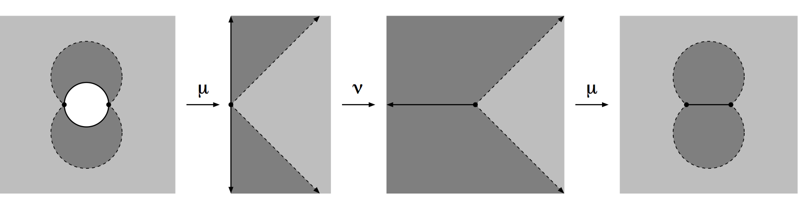
Figure 2. The 3-quasiconformal map that sends the outside of the unit disk to the outside of $[-1,1]$ and identifies conjugate points on the circle. The map is conformal (indeed, is the identity) on the light gray region.

We gave the definition in sectors so that $\sigma$ is conformal off a bounded neighborhood of $\{|z|=1\}$ (it would have been easier to define a 2-quasiconformal map with the same boundary values, but non-conformal in the whole plane). Thus applying $\sigma$ will keep our map holomorphic outside $T(r_{1})$ if $r_{1}$ is large enough.

Note that $\sigma$ maps two conjugate points on the unit circle to the same point of $[-1,1]$, so $\sigma\circ F$ will extend continuously across the edge we are considering. Here $\sigma\circ F$ is applied on the components of the $F$-pre-image of ${\mathbb{C}}\setminus(\{|z|\leq 1\}\cup[1,\infty))$ that contain the relevant edges of $G$ on their boundary, where we note that $\sigma(z)=z$ for $z\in[1,\infty)$.

Finally, given $w\in{\mathbb{D}}=\{|z|<1\}$, we can follow $F$ on a D-component by a quasiconformal map $\rho:{\mathbb{D}}\to{\mathbb{D}}$ so that $\rho(0)=w$, $\rho$ is the identity on $\{|z|=1\}$, and $\rho$ is conformal on $\{|z|<1/2\}$. The QC constant depends only on $|w|$ and blows up as $|w|\nearrow 1$. Then $\rho\circ F$ is uniformly quasiconformal (if $|w|$ is uniformly bounded away from $1$), and has dilatation supported in $T(r)$ for a uniformly bounded $r$ (the maximum of $r$ from Theorem 3.1 and $r_{1}$ above). The choice of $w$ can be different for each D-component, but $|w|$ must be uniformly bounded below $1$ to get a uniform quasiconformal estimate. Thus we have:

Corollary 3.2.

Suppose notation is as above. Given $0<s<1$ there are $r<\infty$ (depending only on the bounded geometry constants of $G$), $K<\infty$ (depending on $s$ and the bounded geometry constants of $G$) and a $K$-quasiregular $g$ on ${\mathbb{C}}$ so that

1. $g=\exp\circ\tau$ off $T(r)$.

2. The center of any D-component with $2n$ boundary vertices is a critical point of order $n$ and each critical value can be specified in $\{|z|<s\}$.

3. The only other singular values of $g$ are $\pm 1$, and the corresponding critical points occur at vertices of $G^{\prime}$.

4. The only asymptotic value is $\infty$, taken in the R-components.

We now adapt the above result to give meromorphic functions. Suppose we have a graph $G$, as above, but now the bounded components (which we still assume are disks) are labeled either as D-components or ID-components (ID for “inverted disk”) and the unbounded components are labeled either as R-components or IR-components (IR for “inverted R-component”). We emphasize that the new terminology ID-component (respectively, IR-component) is introduced only so as to allow a binary labelling of bounded (respectively, unbounded) components of $\mathbb{C}\setminus G$. This enables us, in what follows, to define a quasiregular function $H$ in $\mathbb{C}\setminus G^{\prime}$ so that the definition of $H$ in a given component of $\mathbb{C}\setminus G^{\prime}$ depends on whether that component has been labelled “inverted” or not. We assume that we are given such a labelling so that:

• D-components share edges only with R-components,

• ID-components share edges only with IR-components,

• R-components may share edges with D, R or IR-components,

• IR-components may share edges with ID, R or IR-components.

Apply the Folding Theorem to this graph with ID-components momentarily considered as D-components and IR-components considered as R-components. Obtain the graph extension $G^{\prime}$ of $G$ and the corresponding subdomains of the unbounded components. Each of these is a subset of a R-component or IR-component and they will be called the new R-components and new IR-components.

Next define a function $H$ to be equal to $F$ on the D and new R-components, and only use the QC-map $\sigma$ to modify $F$ on edges with both sides belonging to new R-components (possibly the same component). On the ID and new IR-components we set $H=1/F$, where we only use $\sigma$ to modify $F$ on edges with both sides belonging to new IR-components (possibly the same). Note that this creates poles, but considered as a map into the sphere $H$ is continuous across all edges, except possibly those shared by a new R-component and new IR-component. However, for a point on such an edge, the two possible images of $F$ are conjugate points on the unit circle and since $1/z=\overline{z}$ on the unit circle, $H$ also extends continuously across such edges.

Theorem 3.3.

With the assumptions above, and taking $0<s<1$, there are $r,K<\infty$ (depending only on the bounded geometry constants of $G$; $K$ also may depend on $s$) and a $K$-quasiregular map $g:{\mathbb{C}}\to\widehat{\mathbb{C}}$ that equals $H$ off $T(r)$. Moreover,

1. Each IR-component contains a curve tending to $\infty$ along which $g$ tends to zero; thus each such component contributes an asymptotic value of $0$, which may be perturbed with the map $\rho$.

2. There are $n$ poles (counted with multiplicity) in each ID-component that has $2n$ vertices on its boundary.

3. The critical values corresponding to D-components may be specified independently in $\{|w|<s\}$ and the critical values corresponding to ID-components may be specified independently in $\{|w|>1/s\}$.

4. Constructing the Graph

In this Section we build the graph $G$ that we use in the proof of Theorem 1.1.

Lemma 4.1.

Given $\delta>0$ and an infinite, discrete set of points $\{z_{n}\}$ in the plane, we can construct an unbounded Jordan domain $W$ so that

1. $\{z_{n}\}\subset W$.

2. The points $\{z_{n}\}$ are all at least unit distance apart in the hyperbolic metric for $W$.

3. Every point of $\{z_{n}\}$ lies within a uniformly bounded hyperbolic distance of some fixed hyperbolic geodesic, $\gamma$, for $W$ that connects some finite boundary point $x$ of $W$ to $\infty$.

4. $\operatorname{area}(W)<\delta$ and for all $n\in\mathbb{N}$, ${\rm{area}}(W\cap\{|z|>n\})\leq\delta\exp(-n)$.

5. Every point of the plane lies within distance $1$ of $W$.

6. We can add vertices to $\partial W$ to make it into a uniformly analytic tree with uniformly bounded constants.

7. Each edge $J_{j}$ of this tree is on the boundary of a region $R_{j}\subset W$ so that $\operatorname{area}(R_{j})\simeq\operatorname{diameter}(J_{j})^{2}$ and the $\{R_{j}\}$ are pairwise disjoint.

8. For each edge $J_{j}$ of this tree, the path distance in $W$ from $J_{j}$ to the arc of $\partial W\setminus x$ ($x$ is as in part (3)) that is disjoint from $J_{j}$ is comparable to $\operatorname{diameter}(J_{j})$.

Proof.

The proof is simple and we only sketch the construction, leaving some details for the reader. The main idea is illustrated in Figure 3: we take $W$ to be the union of small, disjoint disks $D_{n}$ centered at the points $\{z_{n}\}$ together with thin polygonal tubes connecting the disks, in order, which leave each disk at antipodal points of the boundary circle. If the connecting tubes are thin compared to the disks, then the points $\{z_{n}\}$ are far apart in the hyperbolic metric, so (2) holds. We now show that (3) follows by imposing an upper bound on the relative entering width of the connecting tubes (described above). Let $x\in\partial W$, $\gamma$ a geodesic in $W$ connecting $x$ to $\infty$, and denote harmonic measure by $\omega$. Let $I_{1},I_{2}$ denote the two components of $\partial W\setminus\{x\}$. Property (3) will follow if we can show that

$$\omega(z_{n},I_{1},W)>c\textrm{ and }\omega(z_{n},I_{2},W)>c$$

for all $n$ and some $c>0$ independent of $n$. By monotonicity properties of harmonic measure we have that

$$\omega(z_{n},I_{1},W)\geq\omega(z_{n},I_{1}\cap\partial D_{n},D_{n}),$$

and $I_{1}\cap\partial D_{n}$ contains a circular arc of harmonic measure (in $D_{n}$) uniformly bounded away from zero given an upper bound on the relative entering width of the connecting tubes. Similar considerations yield the lower bound for $\omega(z_{n},I_{2},W)$.

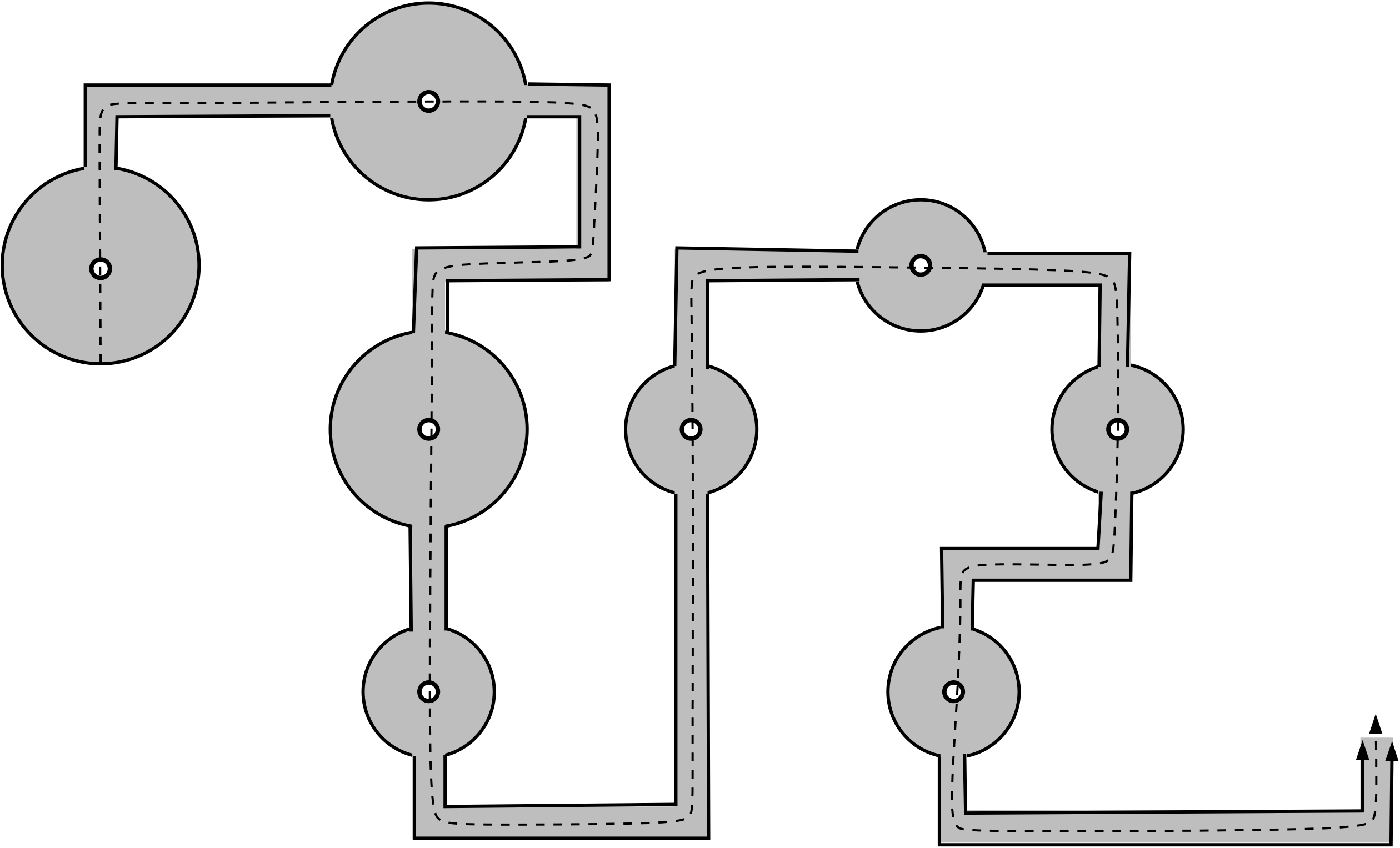
Figure 3. By using small disks around each point and thin corridors that enter and leave on opposite sides of the disks, we can build a Jordan domain that satisfies Lemma 4.1.

Part (4) can be obtained simply by taking the tubes and disks in the construction small enough. To get (5), we can add points to $\{z_{n}\}$ until this set is $1$-dense in the plane, e.g., add any point of $\mathbb{Z}+i\mathbb{Z}$ that does not already have a point of $\{z_{n}\}$ within distance $1/10$ of it. (6) is also easy to verify: on the tubes, take approximately evenly spaced points where the spacing is comparable to the width, and partition the circles in a way that interpolates between the sizes of the two tube openings. If we take a disk centered at the midpoint of $J_{j}$, whose radius is a small multiple of $\operatorname{diameter}(J_{j})$ (depending only on the bounded geometry constants), then the intersection $R_{j}$ of this disk with $W$ satisfies (7). See Figure 4. We can vary the width of a tube (also illustrated in Figure 4) so that all the previous conditions still hold, and the width of a tube when it enters and leaves a disk is always comparable to the width of that disk; thus only a uniformly bounded number (independent of the disk) of vertices is needed on the boundary of each disk and this implies (8) holds.

∎

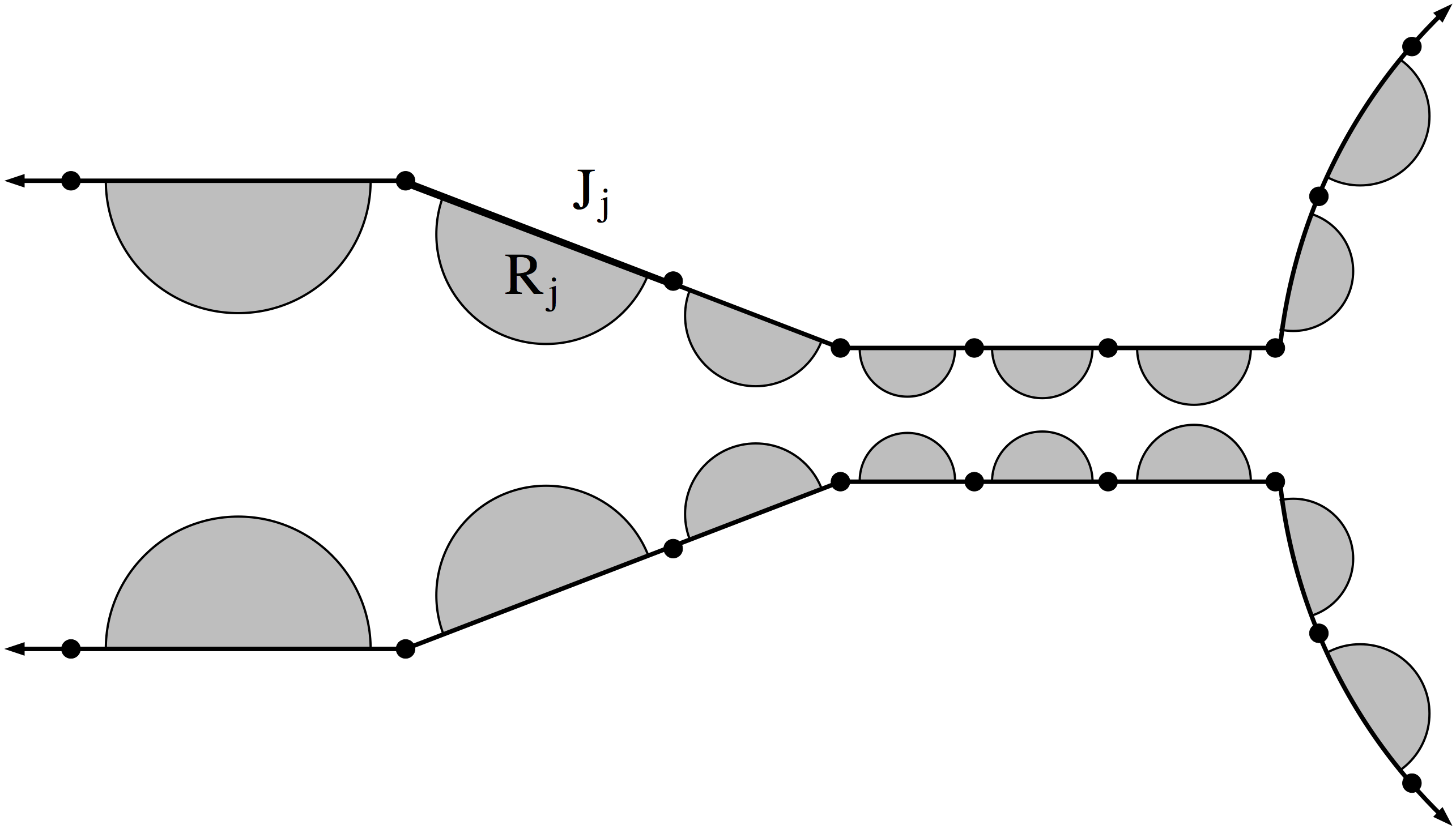
Figure 4. A detail of the tube showing how the tube width can vary, and how to associate a region $R_{j}\subset W$ to each side $J_{j}$ of $W$ so that $\operatorname{area}(R_{j})\simeq\operatorname{diameter}(J_{j})^{2}$.

If we conformally map $W$ to the upper half-plane, we can arrange for the geodesic $\gamma$ of Lemma 4.1 to map to the positive imaginary axis (by mapping the boundary point $x$ in the lemma to the origin; post-composing any conformal map from $W$ to the half-plane taking $\infty$ to $\infty$ with a translation will accomplish this). Then the points $\{z_{n}\}$ map to points in a vertical cone with its vertex at the origin. See Figure 5. Moreover, we can rescale so that the first point has height $1$ above the real axis.

A small disk in $W$ around each $z_{n}$ (say with radius one tenth the distance to the boundary) will map to a near-circular region in the upper half-space and it is easy to connect the near-disks to each other and to $\infty$ to form a bounded geometry graph $\tilde{G}$ as shown in Figure 5. We note that, instead of a bounded component containing the image of $z_{n}$, we may also place a vertex at the image of $z_{n}$, also as shown in Figure 5. The unbounded components are all approximately horizontal half-strips, and it is easy to verify the $\tau$-condition for them. Note that given any labeling of the bounded components by D or ID, we can easily label the unbounded components with R or IR to satisfy the necessary adjacency restrictions.

Figure 5. Building a bounded geometry graph with either a bounded component centered at each point or vertex there.

The bounded geometry and $\tau$-lower bound are clear for all the complementary components of $\tilde{G}$, except possibly the two components that border the real line. These require a separate argument; we want to show the vertices on the real line can be taken with all spacings $\simeq 1$. By the bounded geometry of $\partial W$, the vertices on $\partial W$ map to points on the real line that define a quasisymmetric partition of the line (see Lemma 2.1). Condition (8) of Lemma 4.1 implies that the spacing between the vertices on $\mathbb{R}$ grows exponentially (this is precisely Lemma 8.1 of [3]) and hence the spacing is bounded below. Thus by adding more points to $\tilde{G}$ along the real axis, if necessary, we can assume every edge on the real axis has length at most $1/4$ and without changing the bounded geometry constants of $\tilde{G}$. This verifies the bounded geometry condition and lower $\tau$-bound for the two components that border the real line. Moreover, adding the corresponding vertices to $\partial W$ does not increase the bounded geometry constant or the uniformly analytic constant of $\partial W$.

Therefore, Lemma 4.1 of [3] implies that the image $G$ of $\tilde{G}$ under the conformal map back to $W$ will be a uniformly analytic graph $G$ contained in $\overline{W}$. The $\tau$-condition will be automatically satisfied for components inside $W$, since this is a conformally invariant condition.

These account for all the complementary components of $G$ except for one: the complement $V$ of $\overline{W}$. This is also an unbounded Jordan domain, but it is not clear whether it satisfies the $\tau$-condition. However, there is a very simple trick for fixing this that we take from [3]. Let $\varphi:V\to\mathbb{H}_{u}$ be the conformal map of $V$ to the upper half-plane, taking infinity to infinity. We let $\Phi:\mathbb{H}_{u}\to V$ be its inverse. The vertices on $G$ on $\partial W=\partial V$ map to points on the real line. By Lemma 2.1, these points define a quasisymmetric partition of the real line. We define a graph in the closed upper half-plane by adjoining to the real line vertical rays, and placing evenly spaced vertices on each ray, where the spacing is the minimum distance of that ray to its two neighbors to the left and right. This defines an infinite “comb” tree. See Figure 6.

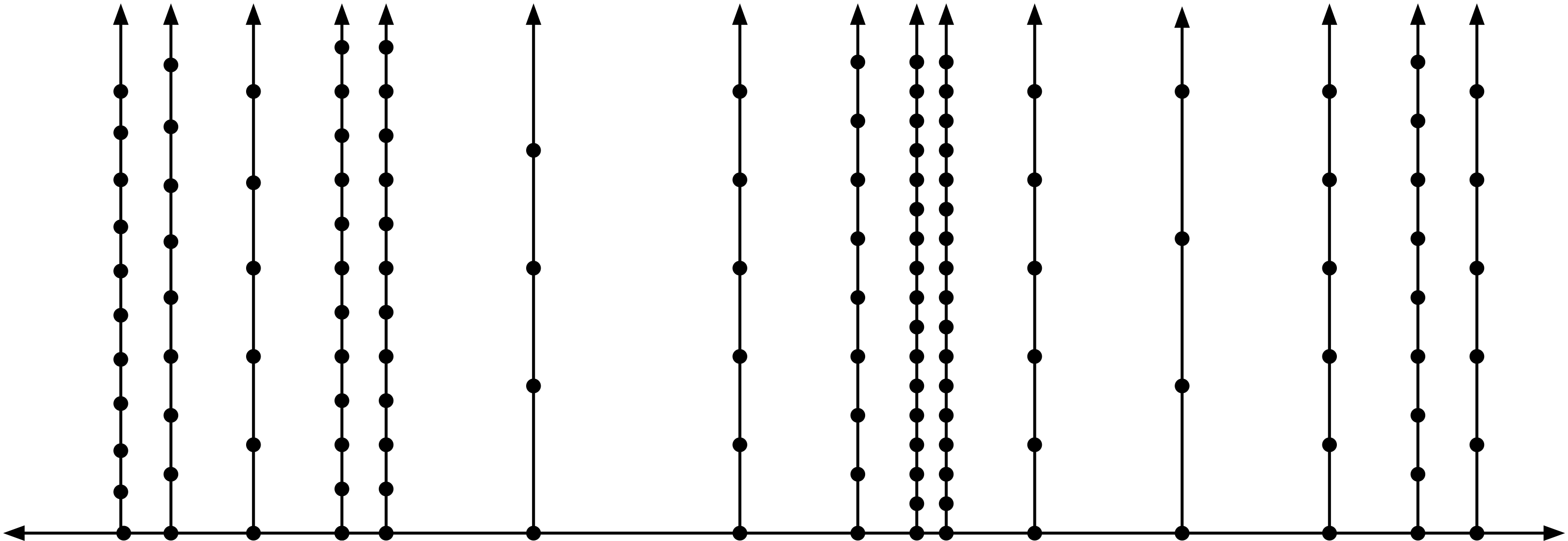
Figure 6. Any quasisymmetric partition of the real line can be extended to a bounded geometry graph in the upper half-plane that satisfies the $\tau$-condition.

By Lemma 6.1 of [3], this tree is uniformly analytic and every component satisfies the $\tau$-condition for an appropriate choice of $\tau$. Therefore by Lemma 4.1 of [3] again, the same is true for the conformal image of this graph in $V$. Adding this image to $G$ gives a new uniformly analytic tree (which we will still call $G$). We mark all the new components (i.e., the subdomains of $V$) as R-components. By construction, these only share edges with the two unbounded sub-domains of $W$ that border $\partial W$, hence they do not share edges with any ID-component, as required in condition (iii) in the discussion preceding Theorem 3.3.

In fact, the $\tau$-condition remains valid for the infinite comb tree even if the spacing of the points decays exponentially in the height. Therefore we can place the vertices so that the graph has bounded geometry, the $\tau$-condition holds on each vertical half-strip, and the area of $T(r)$ intersected with any of the half-strips decays exponentially as we move away from the boundary of the half-plane. Next we use the distortion theorem for conformal maps to prove an analogous estimate for the conformal image of this graph inside $V$.

Lemma 4.2.

Suppose the domain $W$ and graph $G$ are as described above, and that $g$ is the corresponding quasi-regular function given by the folding construction. Let $E$ be the set where $g$ is not holomorphic (note that $E$ is contained in $T(r)$ by construction). There is a $\alpha>0$ so that for any $\delta>0$, we can choose $W$, $G$ and $g$ so that

$$\operatorname{area}(E\cap\{|z|\geq n\})\leq\delta\cdot\exp(-\alpha n),\quad n=0,1,2,\dots$$

Proof.

The domain $W$ was chosen so that $\operatorname{area}(E\cap W)$ satisfies this estimate, so we only need to worry about $\operatorname{area}(E\cap V)=\operatorname{area}(E\setminus\overline{W})$.

We know that $E$ will be contained in the conformal image of the set $T(r)$ corresponding to the comb tree in the upper half-plane illustrated in Figure 6. Recall that $\Phi:\mathbb{H}\to V$ is a conformal map. The tree in the upper half-plane consists of vertical rays that define vertical half-strips $\{S_{j}\}$ with the finite edge $I_{j}$ lying on the real axis. These edges correspond to the edges $\{J_{j}\}$ on $\partial W$ via $\Phi$. In Figure 6, the points on each vertical ray are shown as being evenly spaced, with the spacing being comparable to the distance from the ray to its two neighboring rays. However, we can space the points at height $y$ so they are only separated by distance

(4.1) $$\simeq|I_{j}|\exp(-cy/|I_{j}|),$$

for some $c>0$ and still have the $\tau$-condition. This holds since the conformal map from a half-strip to a half-plane is given in terms of the $\sinh$ function, which has exponential growth in the half-strip (for a single strip we could take $c=\pi$, but since the spacing on a ray depends on the width of both adjacent strips, we use a positive $c$ that depends on the relative sizes of adjacent $I_{j}$’s). See Figure 7; note that the vertical half-strip is drawn horizontally to make the illustration clearer.

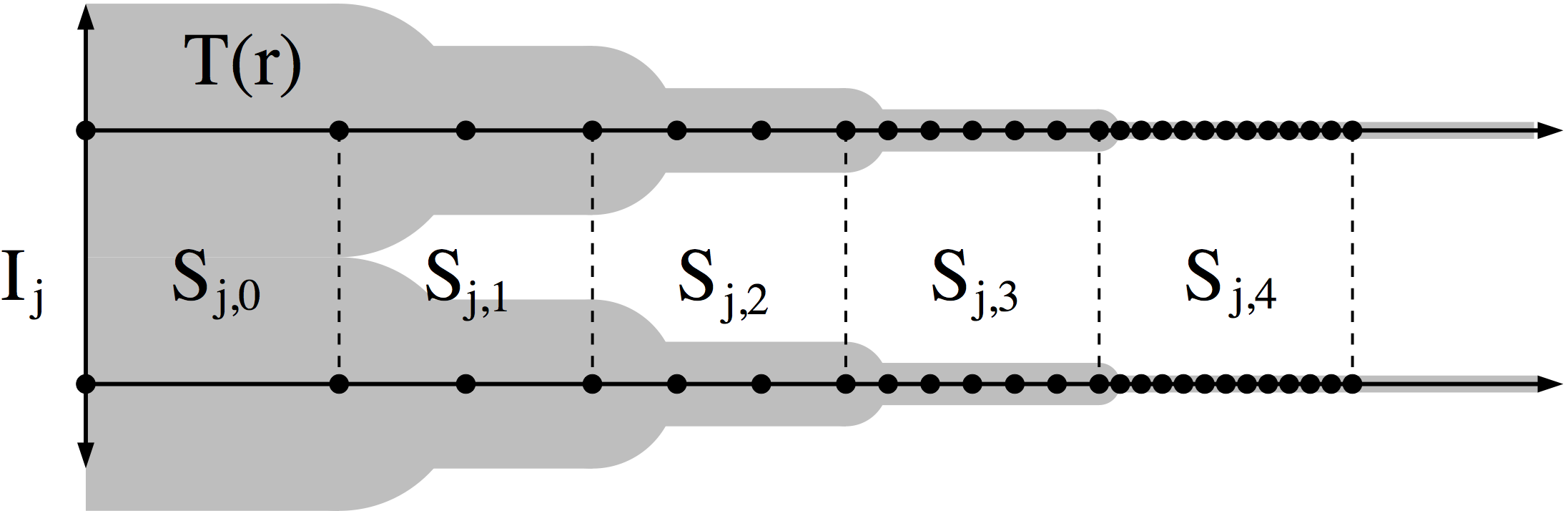
Figure 7. The half-strip $S_{j}$ is cut into squares $\{S_{j,k}\}$ whose intersection with $T(r)$ (shaded) has Euclidean area that decays exponentially with $k$. The picture has been rotated by $90^{\circ}$ compared to Figure 6.

Now cut $S_{j}$ into disjoint squares $\{S_{j,k}\}_{k=0}^{\infty}$ of side length $|I_{j}|$, where $S_{j,k}$ denotes the square whose Euclidean distance from the boundary segment $I_{j}$ is $k|I_{j}|$. Because of the exponential decrease in the spacing between vertices, the fraction of this square that hits $T(r)$ is bounded by $O(\exp(-ck))$ ($c>0$ as in (4.1)). We will show that a similar estimate holds, even after we map these squares back to the region $V$:

Lemma 4.3.

With notation as above,

$$\operatorname{area}(\Phi(T(r)\cap S_{j,k}))\leq C\operatorname{diameter}(J_{j})^{2}\cdot\exp(-ck/2),$$

for $k\geq 0$, where $C<\infty$ is fixed and $c>0$ is as in (4.1).

Proof.

The case $k=0$ (the square that is adjacent to the boundary of the half-plane) is different from the cases $k\geq 1$, and we deal with it first.

Recall that $\varphi:V\to\mathbb{H}_{u}$ is our choice of conformal map and we let $\Phi:\mathbb{H}_{u}\to V$ denote its inverse. In the case $k=0$, we simply bound the area of $\Phi(T(r)\cap S_{j,0})$ by the area of $\Phi(S_{j,0})$ (i.e., we assume $T(r)$ fills the entire square) and we claim the latter set has diameter bounded by a uniform multiple of $\operatorname{diameter}(J_{j})$.

Let $x_{j}$ be the center of the boundary segment $I_{j}$, let $y_{j}=|I_{j}|$ and define $z_{j}=x_{j}+iy_{j}\in\mathbb{H}_{u}$ and $w_{j}=\Phi(z_{j})\in V$. By Koebe’s theorem

(4.2) $$\operatorname{dist}(w_{j},\partial V)\simeq y_{j}|\Phi^{\prime}(z_{j})|,$$

and hence

(4.3) $$y_{j}|\Phi^{\prime}(z_{j})|=O(\operatorname{diameter}(J_{j})),$$

e.g., see Exercise IV.8 in [10].

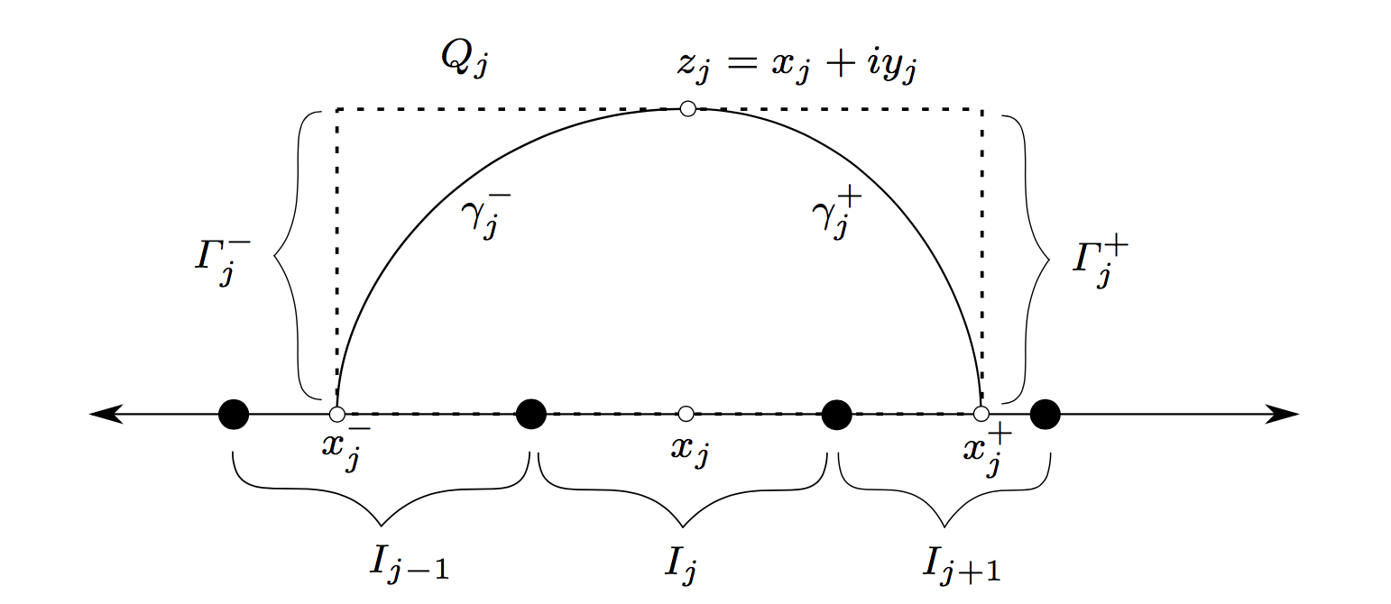
Figure 8. Illustrated is the notation used in the proof of Lemma 4.3 for the case $k=0$.

Assume the boundary intervals $\{I_{j}\}$ are numbered consecutively, so that $I_{j-1}$ and $I_{j+1}$ are adjacent to $I_{j}$. By Lemma 2.1, the intervals $I_{j-1}$, $I_{j}$, $I_{j+1}$ have uniformly comparable lengths (uniform over $j$). Thus by Corollary 4.18 of [15] and (4.2), there exists a point $x_{j}^{-}\in I_{j-1}$ such that the geodesic $\gamma_{j}^{-}$ in $\mathbb{H}_{u}$ with endpoints $x_{j}^{-}$ and $z_{j}$ satisfies

(4.4) $$\textrm{length}(\Phi(\gamma_{j}^{-}))\leq My_{j}\left|\Phi^{\prime}(z_{j})\right|,$$

for $M<\infty$ independent of $j$ (see Figure 8). Let $\Gamma_{j}^{-}$ denote the vertical segment connecting $x_{j}^{-}$ to $x_{j}^{-}+iy_{j}$. We claim that $\Phi(\Gamma_{j}^{-})$ and $\Phi(\gamma_{j}^{-})$ have uniformly comparable lengths (uniform over $j$). To see this, we cut $\Gamma_{j}^{-}$ and $\gamma_{j}^{-}$ into subsegments $\Gamma_{j,k}^{-}$ and $\gamma_{j,k}^{-}$ for $k=0$, $1$, $2$, $\dots$, where the $k^{\textrm{th}}$ subsegment is defined to be the subsegment lying in the horizontal strip

$$\{x+iy:2^{-k-1}y_{j}\leq y\leq 2^{-k}y_{j}\}.$$

Two such subsegments $\Gamma_{j,k}^{-}$, $\gamma_{j,k}^{-}$ lie in a common hyperbolic disc of fixed radius (independent of $j$, $k$), and so by Koebe’s distortion theorem the derivative of $\Phi$ is uniformly comparable throughout this disc. Thus since the lengths of $\Gamma_{j,k}^{-}$, $\gamma_{j,k}^{-}$ are comparable,

$$\textrm{length}(\Phi(\Gamma_{j,k}^{-}))\textrm{ and }\textrm{length}(\Phi(\gamma_{j,k}^{-}))$$

are uniformly comparable (uniform over $j$, $k$). Thus the bound (4.4) implies that

(4.5) $$\textrm{length}(\Phi(\Gamma_{j}^{-}))\leq M^{\prime}y_{j}\left|\Phi^{\prime}(z_{j})\right|$$

for $M^{\prime}<\infty$ independent of $j$. Analogously, there is a point $x_{j}^{+}\in I_{j+1}$ such that the image under $\Phi$ of the vertical segment $\Gamma_{j}^{+}$ connecting $x_{j}^{+}$ to $x_{j}^{+}+iy_{j}$ satisfies a similar bound. Lastly, consider the horizontal segment $l_{j}$ connecting $x_{j}^{-}+iy_{j}$ to $x_{j}^{+}+iy_{j}$. Since $I_{j-1}$, $I_{j}$, $I_{j+1}$ have uniformly comparable lengths,

(4.6) $$\textrm{length}(\Phi(l_{j}))=O(y_{j}\left|\Phi^{\prime}(z_{j})\right|)$$

by Koebe’s distortion theorem. Let $Q_{j}$ be the Euclidean rectangle with vertices $x_{j}^{-}$, $x_{j}^{+}$, $x_{j}^{+}+iy_{j}$, $x_{j}^{-}+iy_{j}$. Summarizing, we have $\Phi(S_{j,0})\subset\Phi(Q_{j})$, and the boundary of the latter set is contained inside the union of $\Phi(\Gamma_{j}^{-})$, $\Phi(\Gamma_{j}^{+})$, $\Phi(l_{j})$, $J_{j-1}$, $J_{j}$, and $J_{j+1}$; all of these have diameter $O(\operatorname{diameter}(J_{j}))$ by (4.3). Thus $\operatorname{diameter}(\Phi(S_{j,0}))=O(\operatorname{diameter}(J_{j}))$, so the $k=0$ case of Lemma 4.3 has been proved.

Next we verify Lemma 4.3 for $k\geq 1$. In this case, $S_{j,k}$ has bounded hyperbolic diameter, so Koebe’s distortion theorem implies

(4.7) $$\frac{\operatorname{area}(\Phi(T(r)\cap S_{j,k}))}{\operatorname{area}(\Phi(S_{j,k}))}\simeq\frac{\operatorname{area}(T(r)\cap S_{j,k})}{\operatorname{area}(S_{j,k})}\simeq\exp(-ck)\textrm{,}$$

where $c>0$ is as in (4.1). Thus it suffices to bound $\operatorname{area}(\Phi(S_{j,k}))$. To do this, we use Lemma 16.1 of [1]:

Proposition 4.4.

Let $\Omega\neq\mathbb{C}$ be simply connected and let $\varphi:\Omega\to\mathbb{H}_{u}$ be a conformal map to the upper half-plane. Let $\Phi:\mathbb{H}_{u}\to\Omega$ denote the inverse of $\varphi$. Let $w=x+it$ and $z=x+iy$ with $y>t$ and let $X\subset\mathbb{H}_{u}$ be a simply connected neigbourhood of $z$ with hyperbolic radius bounded by $r$. Then

$$\operatorname{diameter}(\Phi(X))=O(|\Phi^{\prime}(w)|\frac{y}{t}\operatorname{diameter}(X))$$

where the constant depends only on $r$.

The statement of this in [1] is for the special case $t=1$ and a map into the right half-plane, but the version above follows immediately by considering our $\varphi$ composed with the linear map $z\to-\frac{i}{t}z$. The proof given in [1] is a short deduction from the standard distortion theorem for conformal maps, e.g., Theorem I.4.5 of [10].

We apply Proposition 4.4 using $\varphi$, $t=|I_{j}|=y_{j}$, $w=x_{j}+iy_{j}=z_{j}$ and $X=S_{j,k}$, $k\geq 1$. Note that $y/t=k$ and $\operatorname{diameter}(X)=y_{j}$. Then

$$\operatorname{diameter}(\Phi(X))=O(|\Phi^{\prime}(z_{j})|\cdot k\cdot y_{j}),$$

and using (4.3) gives

$$\operatorname{diameter}(\Phi(X))=O(\operatorname{diameter}(J_{j})\cdot k).$$

Since $k=o(\exp(ck/4))$, we get

$$\operatorname{area}(\Phi(X))=O(\operatorname{diameter}(J_{j})^{2}\exp(ck/2)),$$

and hence, using (4.7),

$$\operatorname{area}(E\cap\Phi(X))=O(\operatorname{diameter}(J_{j})^{2}\exp(-ck/2)),$$

which gives the $k\geq 1$ cases of Lemma 4.3.

∎

Now that Lemma 4.3 is established, we can finish the proof of Lemma 4.2. Let $E_{j}=E\cap\Phi(S_{j})$ and note that

$$\operatorname{area}(E_{j})=\sum_{k=0}^{\infty}\operatorname{area}(E_{j}\cap\Phi(S_{j,k}))=O(\operatorname{diameter}(J_{j})^{2}\sum_{k=0}^{\infty}\exp(-kc/2))=O(\operatorname{area}(R_{j})),$$

where $\{R_{j}\}$ are the regions from Lemma 4.1. Next, let $U_{n}=\{z\in\mathbb{C}:|z|\geq n\}$. Then

$$\operatorname{area}(E\cap U_{n})=\sum_{j}\operatorname{area}(E_{j}\cap U_{n}).$$

We break this sum into two parts, depending on whether $J_{j}$ is contained in $U_{n/2}$ or not. For the first sum, we have

$$\sum_{j:J_{j}\subset U_{n/2}}\operatorname{area}(E_{j})=O(\sum\operatorname{area}(R_{j}))=O(\operatorname{area}(W\cap U_{n/2}))=O(\exp(-n/2)).$$

If $J_{j}$ is not contained in $U_{n/2}$, then let $\gamma_{j}$ be the hyperbolic geodesic connecting the two endpoints of $J_{j}$ inside $V$. Note that $\operatorname{diameter}(\gamma_{j})$ is uniformly bounded from above by a theorem of Gehring and Haymann (see, for instance, Exercise III.16 in [10]) since $\operatorname{diameter}(J_{j})$ is uniformly bounded from above by the construction of $G$. Thus any curve that connects $\gamma_{j}$ to $\partial U_{n}$ inside $V$ has quasi-hyperbolic length at least comparable to $n$ (recall that we have constructed $W$ so that every point of $V$ is within Euclidean distance $1$ of $\partial V$). By Koebe’s distortion theorem, the hyperbolic and quasi-hyperbolic metrics are comparable, and hence the hyperbolic distance from $\gamma_{j}$ to $\partial U_{n}=\{z\in\mathbb{C}:|z|=n\}$ is also comparable to $n$. Thus any square $S_{j,k}$ whose $\Phi$-image hits $U_{n}$ has at least hyperbolic distance $\simeq n$ to $S_{j,0}$ in the upper half-plane and hence $k\geq\exp(an)$ for some fixed $a>0$. Now fix $j$ and sum all over all the squares $S_{j,k}$ whose $\Phi$-images hits $U_{n/2}$:

$$\operatorname{area}(E_{j}\cap U_{n}) \leq \operatorname{area}(R_{j})O(\sum_{k>\exp(an)}\exp(-ck/2))$$

$$\leq \operatorname{area}(R_{j})O(\exp(-acn/2)),$$

for some $a>0$. The $\{R_{j}\}$ are pairwise disjoint and contained in $W$, so summing $\operatorname{area}(R_{j})$ over all $j$ is bounded by $\operatorname{area}(W)$. Taking $\alpha=ac/2$ completes the proof of Lemma 4.2.

∎

We end this Section with the following consequence of Theorem 3.3 and Lemmas 4.1 and 4.2:

Lemma 4.5.

Suppose $\varepsilon,\delta>0$ and suppose we are given an infinite, discrete set of points $\{z_{n}\}_{n=1}^{\infty}$ in the plane, and a sequence $\{w_{n}\}_{n=1}^{\infty}$ so that for each $n$, either $w_{n}=\pm 1$ or $|w_{n}|$ is uniformly bounded away from $1$ (i.e., $||w_{n}|-1|>\varepsilon>0$). Then we can find a quasiregular map $g:{\mathbb{C}}\to\widehat{\mathbb{C}}$ so that:

1. For all $n\in\mathbb{N}$, $g$ has a critical point at $z_{n}$ whose critical value is $w_{n}$.

2. $S(g)=\{w_{n}\}_{n=1}^{\infty}\cup\{\pm 1\}$, i.e., the only other singular values of $g$ are $\pm 1$ (these correspond to the critical points occurring at the vertices of the graph $G^{\prime}$), and the asymptotic value $0$ coming from the IR-components ($0$ can be replaced by any value in $\{|w|<1-\varepsilon\}$).

3. The map $g$ is conformal except on a set $E$ whose area is less than $\delta$, and is exponentially small near $\infty$, i.e., we have ${\rm{area}}(E\cap\{|z|>n\})<\delta\exp(-n)$.

4. Moreover, $K$ does not depend on the particular critical values $\{w_{n}\}$ chosen, but only on $\{z_{n}\}$ and $\varepsilon$.

Proof.

Given the sequences $\{z_{n}\}_{n=1}^{\infty}$ and $\{w_{n}\}_{n=1}^{\infty}$, one obtains a bounded geometry graph $G$ through Lemma 4.1 (and the ensuing discussion in Section 3) with the following property: for each $n\geq 1$, $G$ has a vertex at $z_{n}$ if $w_{n}=\pm 1$, and if $w_{n}\not=\pm 1$, $G$ has a D-component or ID-component centered at $z_{n}$ according to whether $|w_{n}|<1$ or $|w_{n}|>1$, respectively. The bounded geometry constants of $G$ depend only on $\{z_{n}\}_{n=1}^{\infty}$ by Lemmas 4.1 and 4.2. Theorem 3.3 then yields (1), (2) and (4). Property (3) is a consequence of Lemma 4.2.

∎

5. Reducing Theorem 1.1 to a special case

Next we show that it suffices to prove Theorem 1.1 using extra hypotheses on the set $S$.

First, after conjugating by a conformal linear transformation $z\rightarrow az+b$, we may assume $\pm 1\in S$. In other words, given a general $S$ as in Theorem 1.1, we can always find a conformal linear transformation $z\rightarrow m(z)$ so that $\pm 1\in m(S)$. It suffices to find some meromorphic $f$ satisfying the conclusion of Theorem 1.1 for $m(S)$, since then $m^{-1}\circ f\circ m$ is the desired meromorphic function in the conclusion of Theorem 1.1 for the initial $S$.

Next, we claim that since $|S|\geq 4$, we may further always choose the conjugating linear transformation $z\rightarrow m(z)$ so that there is some $s\in S$ with $|m(s)|<1$ in addition to $\pm 1\in m(S)$. Indeed, note that it would suffice to find three points $s,p,q\in S$ so that the circle whose diameter is the straight line segment $[s,p]$ joining $s,p$ contains the third point $q$ in its interior. Moreover, this happens if and only if the angle subtended by $[s,p]$ at $q$ is greater than or equal to $\pi/2$. If three points of $S$ are collinear, the statement is obvious. If we assume a point $r\in S$ is in the interior of the convex hull $T$ of $s,p,q\in S$, then the three angles subtended at $r$ by the three edges of $T$ sum to $2\pi$, hence one of the angles is greater than $\pi/2$, as needed. Lastly, if no point of $s,p,q,r$ is in the convex hull of the other three, then the two segments connecting alternating pairs of points must cross one another. If the closed disk corresponding to each segment does not contain either of the two points of the other pair, the circles must cross in at least four points, which is impossible. Hence we can always choose the conjugating linear transformation $z\rightarrow m(z)$ so that there is some $s\in S$ with $|m(s)|<1$ in addition to $\pm 1\in m(S)$.

Furthermore, we claim that we may further assume that $S$ does not intersect some open neighborhood of $|z|=1$ other than at $\pm 1$. Indeed, suppose for the moment that we can prove Theorem 1.1 for such an $S$. If we then consider the case when $S$ has finitely many points of modulus one, we adjust $S$ by moving each such point of modulus one (other than $\pm 1$) by a radial distance $\varepsilon/2$ inside of $\mathbb{D}$. Then we only need to apply Theorem 1.1 with $\varepsilon/4$ to this adjusted $S$ to obtain the desired result.

Let us return to Theorem 1.1, where we are given $\varepsilon>0$, a discrete sequence $S=(s_{n})$ and some dynamics $h:S\rightarrow S$. By the above discussion, we may assume henceforth that $\pm 1\in S$, there is some $s\in S$ with $|s|<1$, and that $\forall s\in S$ with $s\not=\pm 1$, $||s|-1|>2\varepsilon$. Thus given any sequence $(t_{n}^{*})$ with $|t_{n}^{*}-h(s_{n})|<\varepsilon$ for all $n$ and $t_{n}^{*}=h(s_{n})$ if $h(s_{n})=\pm 1$, we may apply Lemma 4.5 with $\{z_{n}\}=\{s_{n}\}$, $\{w_{n}\}=\{t_{n}^{*}\}$ to yield a quasiregular map $g:\mathbb{C}\rightarrow\hat{\mathbb{C}}$ such that $g$ has a critical point at each $s_{n}$ with corresponding critical value $t_{n}^{*}$. By the measurable Riemann mapping theorem, there exists some quasiconformal map $\phi:\mathbb{C}\rightarrow\mathbb{C}$ such that $f=g\circ\phi^{-1}$ is meromorphic. Moreover, since Lemma 4.5 guarantees that the support of the dilatation of $\phi$ is exponentially small near $\infty$, we may normalize $\phi$ so that $\phi(z)=z+O(1/z)$ near $\infty$ (see for instance [8]). Furthermore, by choosing $\delta$ in Lemma 4.5 sufficiently small, we may guarantee that $|\phi(z)-z|<\varepsilon$ for all $z\in\mathbb{C}$. In the next section we will see how to choose $\{w_{n}\}=\{t_{n}^{*}\}$ so that $\phi^{-1}(t_{n}^{*})=h(s_{n})$ for all $n$.

If we can prove that there is a choice of $\{w_{n}\}=\{t_{n}^{*}\}$ so that $\phi^{-1}(t_{n}^{*})=h(s_{n})$ for all $n$, Theorem 1.1 will be proven in the case that $h$ is onto. Indeed, we would then have $P(f)=S(f)=\{t_{n}^{*}\}$, and $\psi:S\rightarrow P(f)$ defined as $\psi(h(s_{n})):=t_{n}^{*}$ (see also the discussion in Section 1). If $h$ is not onto, the definition $\psi(h(s_{n})):=t_{n}^{*}$ of course does not define $\psi$ on the entirety of $S$ and we may have, for instance, that $|P(f)|=|S(f)|<|S|$. However we claim that in what follows, we may assume that $h$ is onto. Indeed, if $h$ is not onto, we may augment the sequence $S$ with auxiliary points to form a discrete sequence $\tilde{S}$, and extend $h$ to a function $\tilde{h}:\tilde{S}\rightarrow S$ such that $\tilde{h}$ is onto $S$. Then we apply Lemma 4.5 with $\{z_{n}\}=\{\tilde{s}_{n}\}$ and $\{w_{n}\}=\{t_{n}^{*}\}$ where $\{t_{n}^{*}\}$ is any sequence with $|t_{n}^{*}-\tilde{h}(\tilde{s}_{n})|<\varepsilon$ for all $n$ and $t_{n}^{*}=\tilde{h}(\tilde{s}_{n})$ if $\tilde{h}(\tilde{s}_{n})=\pm 1$. Then, again, if we can choose $\{w_{n}\}=\{t_{n}^{*}\}$ so that $\phi^{-1}(t_{n}^{*})=\tilde{h}(\tilde{s}_{n})$ for all $n$, then $f:=g\circ\phi^{-1}$ will be the desired function of Theorem 1.1, with $P(f)=S(f)=\{t_{n}^{*}\}$ and $\psi(\tilde{h}(\tilde{s}_{n})):=t_{n}^{*}$ now defined on all of $S$.

6. Existence of a Fixpoint

With the concluding remarks of Section 1 in mind, we will look for a fixpoint of a self-map of an infinite product of closed Euclidean discs. This fixpoint will correspond to a quasiregular map $g$ so that $g\circ\phi^{-1}$ is the desired meromorphic function in the conclusion of Theorem 1.1. In the previous sections we built a graph $G$ and a quasiregular map $g$ associated to a pair $(S,h)$ from Theorem 1.1. The set of critical points of $g$ included $S$.

The function $g$ depended on a choice of the images of each $s\in S$. We enumerate $S=(s_{i})$. For each choice of $(s_{j}^{*})_{j=1}^{\infty}$ where $s_{j}^{*}\in\overline{D(\varepsilon,s_{j})}$, Lemma 4.5 (and the assumption that $h$ is onto - see Section 5) gives some quasiregular function $g$ with critical points including $S$, and critical values at each $s_{j}^{*}$ where $g(s_{i})=s_{j}^{*}$ if and only if $h(s_{i})=s_{j}$. Thus there is a corresponding quasiconformal map $\phi$ so that $g\circ\phi^{-1}$ is meromorphic. Moreover, we have noted that we can arrange for $|\phi(z)-z|<\varepsilon$ for all $z\in\mathbb{C}$, and $\phi(z)-z=o(1)$ as $z\rightarrow\infty$. Since $\phi(z)-z=o(1)$ as $z\rightarrow\infty$, we can now fix some positive sequence $\varepsilon_{i}\rightarrow 0$ with $\varepsilon_{i}<\varepsilon$ over all $i$, such that $|\phi(s_{i})-s_{i}|<\varepsilon_{i}$, and $(\varepsilon_{i})$ is independent of a choice of $(s_{i}^{*})$.

Lemma 6.1.

With notation as above, the composition of maps

$$\prod_{i=1}^{\infty}\overline{D(\varepsilon_{i},s_{i})}\rightarrow L^{\infty}(\mathbb{C})\rightarrow\prod_{i=1}^{\infty}\overline{D(\varepsilon_{i},s_{i})}$$

given by

(6.1) $$(s_{i}^{*})\rightarrow\mu_{(s_{i}^{*})}\rightarrow(\phi_{\mu_{(s_{i}^{*})}}(s_{i}))$$

is continuous between the product topologies.

Proof.

We recall that a basis for the product topology on $\prod_{i=1}^{\infty}\overline{D(\varepsilon_{i},s_{i})}$ is given by products $\prod_{i=1}^{\infty}U_{i}$ where each $U_{i}$ is open in $\overline{D(\varepsilon_{i},s_{i})}$ and $U_{i}=\overline{D(\varepsilon_{i},s_{i})}$ except for finitely many indices $i$. In particular the topology on $\prod_{i=1}^{\infty}\overline{D(\varepsilon_{i},s_{i})}$ is coarse, and so it is easy to prove continuity of a map into $\prod_{i=1}^{\infty}\overline{D(\varepsilon_{i},s_{i})}$; we only need to check continuity into each factor of the product (see for example Theorem 19.6 of [13]). This is precisely Theorem 1.4. This gives the continuity of the second map in (6.1).

On the other hand, it is slightly more difficult to prove continuity of the first map in (6.1). Fix some sequence $(s_{i}^{*})\in\prod_{i=1}^{\infty}\overline{D(\varepsilon_{i},s_{i})}$ and an open neighborhood $D(r,\mu_{(s_{i}^{*})})\subset L^{\infty}(\mathbb{C})$. We need to find some product of open sets $\prod_{i=1}^{\infty}U_{i}\ni(s_{i}^{*})$ so that $U_{i}=\overline{D(\varepsilon_{i},s_{i})}$ except for finitely many indices $i$, and for any $(t_{i})\in\prod_{i=1}^{\infty}U_{i}$ we have $||\mu_{(t_{i})}-\mu_{(s_{i}^{*})}||_{L^{\infty}(\mathbb{C})}<r$.

Suppose we have indexed $s_{1}^{*}$ as the unique asymptotic value of $g$, and consider some fixed $i>1$. Varying $s_{i}^{*}$ changes the dilatation of $g$ only on a collection of thin annuli $A_{j}\subset D_{j}$ for which $h(s_{j})=s_{i}$. Let $E_{i}$ be the union of those annuli $A_{j}\subset D_{j}$ for which $h(s_{j})=s_{i}$. For $s_{1}^{*}$, we define $E_{1}$ as $T(r_{0})\setminus(\cup_{s}D_{s})$ in union with any $A_{j}\subset D_{j}$ for which $h(s_{j})=s_{1}$; the reason for this definition is that varying $s_{1}^{*}$ changes the dilatation of $g$ only on $E_{1}$.

Now consider some fixed $E_{j}$. Then $\mu_{(t_{i})}|_{E_{j}}$ depends only on $t_{j}$, and as $t_{j}\rightarrow s_{j}^{*}$, it is clear that $\mu_{(t_{i})}|_{E_{j}}\rightarrow\mu_{(s_{i}^{*})}|_{E_{j}}$ uniformly, so that we may choose some $\delta>0$ with $||\mu_{(t_{i})}-\mu_{(s_{i}^{*})}||_{L^{\infty}(E_{j})}<r$ as long as $t_{j}\in\overline{D(\delta,s_{j}^{*})}$. Since $\varepsilon_{j}\rightarrow 0$, we know that for all sufficiently large $j$ we have $D(\varepsilon_{j},s_{j})\subset D(\delta,s_{j}^{*})$, and we choose $U_{j}=\overline{D(\varepsilon_{j},s_{j})}$ for such $j$. For the finitely many other indices $j$, we choose $U_{j}=D(\delta,s_{j}^{*})\cap\overline{D(\varepsilon_{j},s_{j})}$. With this choice of $\prod_{i=1}^{\infty}U_{i}$, we have that $||\mu_{(t_{i})}-\mu_{(s_{i}^{*})}||_{L^{\infty}(\mathbb{C})}<r$ for any $(t_{i})\in\prod_{i=1}^{\infty}U_{i}$, as required.

∎

We are now ready to prove Theorem 1.1. We remark that the singular values $\pm 1$ are distinguished from other singular values of $g$ in that we do not have the freedom in Lemma 4.5 to perturb $\pm 1$. Therefore, the proof is simpler in the case when the correction map $\phi$ fixes both $\pm 1$. We will first prove the theorem in this case, and then extend the argument to cover the general case.

Theorem 1.1 assuming $\phi$ fixes $\pm 1$.

We have just shown that the map in (6.1) is continuous and maps $\prod_{i=1}^{\infty}\overline{D(\varepsilon_{i},s_{i})}$ into itself; this was arranged by definition of $\varepsilon_{i}$. Thus Theorem 1.3 implies this map has fixpoint. A fixpoint of (6.1) corresponds to some choice of $(s_{i}^{*})$ so that $\phi^{-1}_{\mu_{(s_{i}^{*})}}(s_{i}^{*})=s_{i}$ for all singular values other than $\pm 1$. By assumption this also holds if we set $(1)^{*}=1$ and $(-1)^{*}=-1$. If $f(z)=g(\phi^{-1}(z))$, then $f$ is meromorphic and we have $f|_{S^{*}}=\psi\circ h\circ\psi^{-1}$, where the map $\psi$ is defined by $\psi(s)=s^{*}$. This proves Theorem 1 under the extra assumption that $\phi^{-1}$ fixes both $\pm 1$.

∎

Theorem 1.1 in general.

Now we consider the case when the correction map $\phi^{-1}$ does not necessarily fix both $\pm 1$. Let $\delta>0$ be the distance from $\pm 1$ to the remainder of the singular set (this is positive since the singular set is discrete). For each $x,y\in\overline{D(-1,\delta/2)}\times\overline{D(1,\delta/2)}$ let $\eta$ be a quasiconformal map so that $\eta(-1)=x$, $\eta(1)=y$ and $\eta$ is the identity outside $U=D(-1,\delta)\cup D(1,\delta)$. Clearly we can do this with a dilation that is uniformly bounded independent of $\delta$, $x$ and $y$ and is supported inside $U$.

We now wish to repeat the fixpoint argument above with $g$ replaced by $G=\eta\circ g$. This is still a quasi-regular map that depends on the parameters $\{s_{j}^{*}\}$ and two new parameters $x,y$. The $g$ preimages of $U$ are contained in $T(r)$ for a uniform choice of $r$, so $G$ still has a dilatation that is supported in a set of small area and this area decays exponentially near $\infty$. Therefore the corresponding correction map $\phi$ still varies continuously in all the parameters. Moreover, $\phi$ will move each of the points $\pm 1$ by as little as we wish, depending on our choice of $W$. Therefore we can arrange for $\phi$ to map $-1$ into $\overline{D(-1,\delta/2)}$ for any $x\in\overline{D(-1,\delta/2)}$, independent of how the other parameters are chosen. Similarly, $\phi$ maps $1$ into $\overline{D(1,\delta/2)}$. The chosen closed disks around all the other (non $\pm 1$) singular values still map into themselves as before, so the fixpoint argument from above applies again. More precisely, there is a choice of $x\in\overline{D(-1,\delta/2)}$, $y\in\overline{D(1,\delta/2)}$, and $\{s_{j}^{*}\}\in\overline{D(s_{j},\varepsilon_{j})}$ so that $\phi(-1)=x$, $\phi(1)=y$, and $\phi(s_{j})=s_{j}^{*}$ for all $j$.

Let $f(z)=\eta(g(\phi^{-1}(z)))$. Then the definition of $\eta$ implies

$$f(x)=\eta(g(\phi^{-1}(x)))=\eta(g(-1))=\begin{cases}x&\mbox{ if }g(-1)=-1,\\ y&\mbox{ if }g(-1)=1,\\ g(-1)&\mbox{ otherwise. }\end{cases}$$

Similarly for $f(y)$. For other $s_{j}\in S$ such that $s_{j}\not=\pm 1$, we have $\eta(s_{j})=s_{j}$ (since $\eta$ is the identity away from $\pm 1$), so

$$f(s_{j}^{*})=\eta(g(\phi^{-1}(s_{j}^{*})))=\eta(g(s_{j}))=\begin{cases}x&\mbox{ if }g(s_{j})=-1,\\ y&\mbox{ if }g(s_{j})=1,\\ g(s_{j})&\mbox{ otherwise. }\end{cases}$$

Thus if we set $\psi(-1)=x$, $\psi(1)=y$ and $\psi(s_{j})=s_{j}^{*}$ for the other singular values, then $f,\psi$ satisfy the conclusions of Theorem 1.1.

∎

References

- [1] Albrecht, S., Bishop, C.J.: Spieser class Julia sets with dimension near one. preprint (2017)
- [2] Bishop, C.J.: Constructing entire functions by quasiconformal folding. Acta Math. 214(1), 1–60 (2015). DOI 10.1007/s11511-015-0122-0. URL http://dx.doi.org/10.1007/s11511-015-0122-0
- [3] Bishop, C.J.: Models for the Speiser class. Proc. Lond. Math. Soc. (3) 114(5), 765–797 (2017). DOI 10.1112/plms.12025. URL https://doi.org/10.1112/plms.12025
- [4] Carleson, L., Gamelin, T.W.: Complex dynamics. Universitext: Tracts in Mathematics. Springer-Verlag, New York (1993). DOI 10.1007/978-1-4612-4364-9. URL https://doi.org/10.1007/978-1-4612-4364-9
- [5] L.G. DeMarco, S.C. Koch, and C.T. McMullen. On the postcritical set of a rational map. Mathematische Annalen, Aug 2018.
- [6] N. Fagella, X. Jarque, and K. Lazebnik. Univalent Wandering Domains in the Eremenko-Lyubich Class. arXiv e-prints, page arXiv:1711.10629, Nov 2017.
- [7] D. Martí-Pete and M. Shishikura. Wandering domains for entire functions of finite order in the Eremenko-Lyubich class. arXiv e-prints, July 2018.
- [8] Dyn’ kin, E.M.: Smoothness of a quasiconformal mapping at a point. Algebra i Analiz 9(3), 205–210 (1997)
- [9] Fagella, N., Godillon, S., Jarque, X.: Wandering domains for composition of entire functions. J. Math. Anal. Appl. 429(1), 478–496 (2015). DOI 10.1016/j.jmaa.2015.04.020. URL http://dx.doi.org/10.1016/j.jmaa.2015.04.020
- [10] Garnett, J., Marshall, D.: Harmonic measure, New Mathematical Monographs, vol. 2. Cambridge University Press (2005)
- [11] Lazebnik, K.: Several constructions in the Eremenko-Lyubich class. J. Math. Anal. Appl. 448(1), 611–632 (2017). DOI 10.1016/j.jmaa.2016.11.007. URL http://dx.doi.org/10.1016/j.jmaa.2016.11.007
- [12] Lazebnik, K. Oscillating Wandering Domains for Functions with Escaping Singular Values. arXiv e-prints, April 2019.
- [13] Munkres, J.R.: Topology: a first course. Prentice-Hall, Inc., Englewood Cliffs, N.J. (1975)
- [14] Osborne, J.W., Sixsmith, D.J.: On the set where the iterates of an entire function are neither escaping nor bounded. Ann. Acad. Sci. Fenn. Math. 41(2), 561–578 (2016)
- [15] Ch. Pommerenke. Boundary behaviour of conformal maps, volume 299 of Grundlehren der Mathematischen Wissenschaften [Fundamental Principles of Mathematical Sciences]. Springer-Verlag, Berlin, 1992.
- [16] Rempe-Gillen, L.: Arc-like continua, Julia sets of entire functions, and Eremenko’s conjecture. preprint (2016)
- [17] Sixsmith, D.J.: Dynamics in the Eremenko-Lyubich class. ArXiv e-prints (2017)
- [18] Tychonoff, A.: Ein Fixpunktsatz. Math. Ann. 111(1), 767–776 (1935). URL https://doi.org/10.1007/BF01472256