A Lawson-type exponential integrator for the Korteweg–de Vries equation

Abstract

We propose an explicit numerical method for the periodic Korteweg–de Vries equation. Our method is based on a Lawson-type exponential integrator for time integration and the Rusanov scheme for Burgers’ nonlinearity. We prove first-order convergence in both space and time under a mild Courant–Friedrichs–Lewy condition $\tau=O(h)$, where $\tau$ and $h$ represent the time step and mesh size, respectively, for solutions in the Sobolev space $H^{3}((-\pi,\pi))$. Numerical examples illustrating our convergence result are given.

Keywords. exponential integrators; Lawson methods; Korteweg–de Vries equation; error estimates; Rusanov scheme

1 Introduction

Consider the Korteweg–de Vries (KdV) equation

$$u_{t}+u_{xxx}+uu_{x}=0,\quad x\in\Omega=(-\pi,\pi),\quad t>0,$$ (1.1)

$$u(x,0)=u_{0}(x),\quad x\in\overline{\Omega},$$

where we impose periodic boundary conditions for practical implementation. The KdV  equation is a generic model for the study of weakly nonlinear long waves. It describes the propagation of shallow water waves in a channel [23] and is widely applied in science and engineering, such as in plasma physics where it gives rise to ion acoustic solitons [8] and in geophysical fluid dynamics where it describes long waves in shallow seas and deep oceans [29, 30]. The KdV equation is also relevant for studying the interaction between nonlinearity and dispersion.

For the well-posedness of the periodic KdV equation, we refer to [4, 6, 12]. It was shown in [6] that the equation is globally well-posed for initial data in $H^{s}(\Omega)$ with $s\geq-1/2$. For its numerical solution, various methods have been proposed and analyzed in the literature, such as finite difference methods (FDM) [38, 36, 13, 19], finite element methods [1, 39, 9, 2], Fourier spectral methods [5, 28, 33, 31, 32], splitting methods [18, 21, 17] and Petrov–Galerkin methods for the KdV equation with nonperiodic boundary condition [26, 27, 34]. Numerical methods for the Kadomtsev–Petviashvili equation, which is a two-dimensional generalization of the KdV equation, were considered in [10, 22].

For finite difference methods, linear stability has been analyzed in [11, 36, 38]. The explicit leap-frog scheme [36] and the Lax–Friedrichs scheme [38] require both the rather severe stability condition $\tau=O(h^{3})$, where $\tau$ and $h$ represent the discretization parameters in time and space, respectively. To weaken the stability restriction, some implicit FDM were proposed in [11, 36]. Recently, the Lax–Friedrichs scheme with an implicit dispersion was proved to converge uniformly to the solution of the KdV equation for initial data in $H^{3}$ under the stability condition $\tau=O(h^{3/2})$ for both the decaying case on the full line and the periodic case [19]. However, no convergence rate was obtained. Very recently, for the $\theta$-right winded FDM, which applies the Rusanov scheme for the hyperbolic flux term and a 4-point $\theta$-scheme for the dispersive term, first-order convergence in space was proved under a hyperbolic Courant–Friedrichs–Lewy (CFL) condition $\tau=O(h)$ for $\theta\geq\frac{1}{2}$ and under an Airy Courant–Friedrichs–Lewy condition $\tau=O(h^{3})$ for $\theta<\frac{1}{2}$, for solutions in $H^{6}(\mathbb{R})$ [7].

On the other hand, the numerical approximation by Fourier spectral/pseudospectral methods has been studied by many authors [28, 25]. Maday and Quarteroni [28] showed that for solutions in $H^{r}$, the error of the Fourier spectral method is of order $O(h^{r-1})$ in the $L^{2}$ norm while the error of the pseudospectral method is of order $O(h^{r-2})$ in the $H^{1}$ norm. The corresponding $L^{2}$ estimate for the Fourier pseudospectral method was established in [25] with the aid of artificial viscosity to avoid the nonlinear instability caused by the aliasing error. More specifically, first-order convergence in time was shown in [25] for the fully discrete pseudospectral method under the stability condition $\tau=O(h^{3})$ for explicit and $\tau=O(h^{2})$ for implicit discretization of the nonlinear term, respectively. For the rigorous analysis of splitting methods, we refer to [17, 20].

Nowadays, exponential time integration methods are widely applied for parabolic and hyperbolic problems [15, 16, 3]. In particular, a distinguished exponential-type integrator was derived for the KdV equation [16] by using a “twisting” technique. For this integrator, first-order convergence in time was proved without any CFL condition required. However, the success of this scheme strongly depends on the particular form of the equation. The resulting key relation $k_{1}^{3}+k_{2}^{3}-(k_{1}+k_{2})^{3}=-3(k_{1}+k_{2})k_{1}k_{2}$ in Fourier space allows one to integrate the stiff part involving $\partial_{x}^{3}$ exactly without loss of regularity. Such an integrator, however, can hardly be extended to more general equations, e.g., the fifth-order KdV equation, without additional regularity assumptions. Furthermore, the spatial error was not considered in [16].

In the present paper, we propose a Fourier pseudospectral method based on a classical Lawson-type exponential integrator, which integrates the linear part exactly, and the Rusanov scheme for Burgers’ nonlinearity with an added artificial viscosity. The method is explicit, implemented with FFT and efficient in practical computation. First-order convergence in both space and time is shown under a mild CFL condition $\tau=O(h)$. Moreover, the method can be easily extended to other dispersive equations with Burgers’ nonlinearity.

The rest of this paper is organized as follows. In Section 2, we present the necessary notation, the numerical scheme and the main convergence result. Section 3 is devoted to the details of the error analysis. Numerical results are reported in Section 4 to illustrate our error bounds.

Throughout the paper, $C$ represents a generic constant, which is independent of the discretization parameters and the exact solution $u$.

2 The Fourier pseudospectral method

We adopt the standard Sobolev spaces and denote by $\|\cdot\|$ and $(\cdot,\cdot)$ the norm and inner product in $L^{2}(\Omega)$, respectively. For $m\in\mathbb{N}$, we denote by $H_{\rm p}^{m}(\Omega)$ the $H^{m}$ functions on the one-dimensional torus $\Omega=(-\pi,\pi)$. In particular, these functions have derivatives up to order $m-1$ that are all $2\pi$-periodic. The space is equipped with the standard norm $\|\cdot\|_{m}$ and semi-norm $|\cdot|_{m}$.

Let $\tau=\Delta t>0$ be the time step size and denote the temporal grid points by $t_{k}:=k\tau$ for $k=0,1,2,\ldots$. Given a mesh size $h:=2\pi/(2N+1)$ with $N$ being a positive integer, let

$$x_{j}:=-\pi+jh,\qquad j=0,1,\ldots,2N,$$

be the spatial grid points in $[-\pi,\pi)$. Denote

$$X_{N}:=\mathrm{span}\left\{e^{ikx}:|k|\leq N\right\},\qquad\qquad\qquad\,\widetilde{X}_{N}:=\left\{v=\sum\limits_{k=-N}^{N}v_{k}e^{ikx}\in\mathbb{R}\right\}\subseteq X_{N},$$

$$Y_{N}:=\left\{v=(v_{0},v_{1},\ldots,v_{{}_{2N}})\in\mathbb{C}^{2N+1}\right\},\qquad\widetilde{Y}_{N}=Y_{N}\cap\mathbb{R}^{2N+1}.$$

For any $u,v\in C(\Omega)$, define the following discrete inner product and norm by

$$\langle u,v\rangle_{{}_{N}}=h\sum\limits_{j=0}^{2N}u(x_{j})\overline{v(x_{j})},\qquad\interleave u\interleave_{{}_{N}}=\langle u,u\rangle_{{}_{N}}^{1/2}.$$

For a periodic function $v(x)$ and a vector $v\in Y_{N}$, let $P_{N}:L^{2}(\Omega)\rightarrow X_{N}$ be the standard orthogonal projection operator, and $I_{N}:C(\Omega)\rightarrow X_{N}$ or $I_{N}:Y_{N}\rightarrow X_{N}$ be the interpolation operator [35], i.e.,

$$(P_{N}v,\varphi)=(v,\varphi),\quad\mathrm{for}\ \ \mathrm{all}\quad\varphi\in X_{N};$$

$$(I_{N}v)(x_{j})=v(x_{j}),\quad\mathrm{or}\quad(I_{N}v)(x_{j})=v_{j},\quad j=0,\ldots,2N.$$

More specifically, $P_{N}v$ and $I_{N}v$ can be written as

$$(P_{N}v)(x)=\sum\limits_{l=-N}^{N}\widehat{v}_{l}e^{ilx},\quad(I_{N}v)(x)=\sum\limits_{l=-N}^{N}\widetilde{v}_{l}e^{ilx},$$

where $\widehat{v}_{l}$ and $\widetilde{v}_{l}$ are the Fourier and discrete Fourier coefficients, respectively, defined as

$$\widehat{v}_{l}=\frac{1}{2\pi}\int_{0}^{2\pi}v(x)e^{-ilx}dx,\qquad\widetilde{v}_{l}=\frac{1}{2N+1}\sum\limits_{j=0}^{2N}v_{j}e^{-ilx_{j}},\quad l=-N,\dots,N.$$

It was proved in [35] that for any $u,v\in C(\Omega)$,

$$\langle u,v\rangle_{{}_{N}}=(I_{N}u,I_{N}v),\qquad\interleave u\interleave_{{}_{N}}=\|I_{N}u\|.$$ (2.1)

The semi-discrete pseudospectral method for (1.1) consists in finding $u_{{}_{N}}$ in $\widetilde{X}_{N}$ such that

$$\partial_{t}u_{{}_{N}}(x,t)+\partial_{x}^{3}u_{{}_{N}}(x,t)+\frac{1}{2}I_{N}\left((u_{{}_{N}}^{2})_{x}\right)(x,t)=0,\quad x\in\Omega=(-\pi,\pi),\quad t>0,$$ (2.2)

$$u_{{}_{N}}(x,0)=I_{N}(u_{0})(x),\quad x\in\overline{\Omega}.$$

Thus, by Duhamel’s formula, we have

$$u_{{}_{N}}(t_{n}+\tau)=e^{-\tau\partial_{x}^{3}}u_{{}_{N}}(t_{n})-\frac{1}{2}\int_{0}^{\tau}e^{-(\tau-s)\partial_{x}^{3}}I_{N}\left((u_{{}_{N}}^{2})_{x}(t_{n}+s)\right)ds.$$

By applying the approximation $u_{{}_{N}}(t_{n}+s)\approx u_{{}_{N}}(t_{n})$ and the first-order Lawson method [24, 14], we get a first-order approximation as

$$u_{{}_{N}}(t_{n}+\tau)\approx e^{-\tau\partial_{x}^{3}}u_{{}_{N}}(t_{n})-\frac{\tau}{2}e^{-\tau\partial_{x}^{3}}I_{N}\left((u_{{}_{N}}^{2})_{x}(t_{n})\right).$$ (2.3)

To ensure the stability, we apply the Rusanov scheme [37, 7] for Burgers’ nonlinearity, which consists of a centered hyperbolic flux and an added artificial viscosity. The scheme then reads as

$$\begin{split}&u_{{}_{N}}^{n+1}=e^{-\tau\partial_{x}^{3}}u_{{}_{N}}^{n}-\frac{\tau}{2}e^{-\tau\partial_{x}^{3}}I_{N}\delta_{x}^{0}\left((u_{{}_{N}}^{n})^{2}\right)+\frac{c\tau h}{2}e^{-\tau\partial_{x}^{3}}\delta_{x}^{2}u_{{}_{N}}^{n},\quad n\geq 0,\\ &u_{{}_{N}}^{0}=I_{N}(u_{0}),\end{split}$$ (2.4)

where the constant $c$ is the so-called Rusanov coefficient, which has to satisfy a certain condition (cf. (3.29)). Moreover, we have used the notation

$$\delta_{x}^{0}v(x)=\frac{v(x+h)-v(x-h)}{2h},\quad\delta_{x}^{2}v(x)=\frac{v(x+h)-2v(x)+v(x-h)}{h^{2}},$$

where $v(x)=v(x\pm 2\pi)$. Similarly, for a vector $v\in Y_{N}$, define the standard finite difference operators as

$$\delta_{x}^{0}v_{j}=\frac{v_{j+1}-v_{j-1}}{2h},\quad\delta_{x}^{2}v_{j}=\frac{v_{j+1}-2v_{j}+v_{j-1}}{h^{2}},\quad\delta_{x}^{+}v_{j}=\frac{v_{j+1}-v_{j}}{h},\quad j=0,1,\dots,2N,$$

with $v_{j\pm(2N+1)}=v_{j}$ when necessary.

We are now in the position to present the main result of the paper.

Theorem 2.1

Assume that the solution of (1.1) satisfies $u\in C(0,T;H_{\rm p}^{3}(\Omega))$ and let $c_{0}>0$ be given by condition (3.29). Then, for $c>c_{0}$, there exists $h_{0}>0$ such that for all $h\leq h_{0}$ and $\tau\leq h/c$, the error of scheme (2.4) satisfies

$$\|u_{{}_{N}}^{n}-u(t_{n})\|\leq M(\tau+h),\qquad n\tau\leq T.$$ (2.5)

Here both of the constants $M$ and $h_{0}$ depend on $T$, $c$ and $\|u\|_{L^{\infty}(0,T;H_{\rm p}^{3}(\Omega))}$ (cf. (3.31) and (3.30)).

3 Error estimate

The purpose of this section is to prove Theorem 2.1.

3.1 Some lemmas

We recall three lemmas from the literature and then prove an additional lemma. All the lemmas are used in the proof of Theorem 2.1.

Lemma 3.1

[35]. For any $u\in H_{\rm p}^{m}(\Omega)$ and $0\leq\mu\leq m$,

$$\|P_{N}u-u\|_{\mu}\leq Ch^{m-\mu}|u|_{m},\quad\|P_{N}u\|_{m}\leq C\|u\|_{m}.$$ (3.1)

In addition, if $m>\frac{1}{2}$, then

$$\|I_{N}u-u\|_{\mu}\leq Ch^{m-\mu}|u|_{m},\quad\|I_{N}u\|_{m}\leq C\|u\|_{m}.$$ (3.2)

Lemma 3.2 (Nikolski’s Inequality)

[35]. For any $u\in X_{N}$ and $1\leq p\leq q\leq\infty$,

$$\|u\|_{L^{q}}\leq\left(\frac{Np_{0}+1}{2\pi}\right)^{\frac{1}{p}-\frac{1}{q}}\|u\|_{L^{p}},$$

where $p_{0}$ is the smallest even integer $\geq p$. In particular, for $p=2$ and $q=\infty$, we have

$$\|u\|_{L^{\infty}}\leq h^{-1/2}\|u\|.$$ (3.3)

Lemma 3.3 (Bernstein’s Inequality)

[35]. For any $u\in X_{N}$ and $0\leq\mu\leq m$,

$$\|u\|_{m}\leq Ch^{\mu-m}\|u\|_{\mu}.$$ (3.4)

Lemma 3.4

For $a=(a_{0},a_{1},\ldots,a_{{}_{2N}})$, $b=(b_{0},b_{1},\ldots,b_{{}_{2N}})\in\widetilde{Y}_{N}$, we have

$$\langle a,\delta_{x}^{2}b\rangle_{{}_{N}}=-\langle\delta_{x}^{+}a,\delta_{x}^{+}b\rangle_{{}_{N}},$$ (3.5)

and

$$\sum\limits_{j=0}^{2N}\left(\delta_{x}^{2}a_{j}\right)^{2}=\frac{4}{h^{2}}\sum\limits_{j=0}^{2N}\left[\left(\delta_{x}^{+}a_{j}\right)^{2}-\left(\delta_{x}^{0}a_{j}\right)^{2}\right],$$ (3.6)

$$\sum\limits_{j=0}^{2N}a_{j}a_{j+1}\delta_{x}^{+}a_{j}=-\frac{h^{2}}{3}\sum\limits_{j=0}^{2N}(\delta_{x}^{+}a_{j})^{3},\qquad\qquad\sum\limits_{j=0}^{2N}a_{j-1}a_{j+1}\delta_{x}^{0}a_{j}=-\frac{4h^{2}}{3}\sum\limits_{j=0}^{2N}(\delta_{x}^{0}a_{j})^{3},$$ (3.7)

$$\sum\limits_{j=0}^{2N}\delta_{x}^{2}a_{j}\delta_{x}^{0}(ab)_{j}=-\frac{1}{h^{2}}\sum\limits_{j=0}^{2N}a_{j}a_{j+1}\delta_{x}^{+}b_{j}+\frac{1}{h^{2}}\sum\limits_{j=0}^{2N}a_{j-1}a_{j+1}\delta_{x}^{0}b_{j}.$$ (3.8)

Proof. The identity (3.5) is the discrete version of the integration by parts formula:

$$\langle a,\delta_{x}^{2}b\rangle_{{}_{N}} =\frac{1}{h}\sum\limits_{j=0}^{2N}a_{j}(b_{j+1}-2b_{j}+b_{j-1})=\frac{1}{h}\sum\limits_{j=0}^{2N}a_{j}(b_{j+1}-b_{j})-\frac{1}{h}\sum\limits_{j=0}^{2N}a_{j}(b_{j}-b_{j-1})$$

$$=\sum\limits_{j=0}^{2N}a_{j}\delta_{x}^{+}b_{j}-\sum\limits_{j=0}^{2N}a_{j+1}\delta_{x}^{+}b_{j}=-h\sum\limits_{j=0}^{2N}(\delta_{x}^{+}a_{j})(\delta_{x}^{+}b_{j})=-\langle\delta_{x}^{+}a,\delta_{x}^{+}b\rangle_{{}_{N}}.$$

The equalities (3.6)-(3.8) were established in [7] for infinite sequences. By applying the same arguments, we can get (3.6)-(3.8) for periodic sequences here. We refer to [7] for details. $\square$

3.2 Local error analysis

We introduce the local truncation error $\xi^{n+1}$ as defect

$$\xi^{n+1}=u(t_{n+1})-e^{-\tau\partial_{x}^{3}}u(t_{n})+\frac{\tau}{2}e^{-\tau\partial_{x}^{3}}\left[\delta_{x}^{0}(u(t_{n})^{2})-ch\delta_{x}^{2}u(t_{n})\right],\quad n\geq 0.$$ (3.9)

The local error can be bounded as follows.

Lemma 3.5

For $u\in C(0,T;H_{\rm p}^{3}(\Omega))$, we have

$$\|\xi^{n+1}\|\leq M_{3}\tau^{2}+M_{2}\tau h,$$

where $M_{3}$ and $M_{2}$ depend on $\|u\|_{L^{\infty}(0,T;H^{3}(\Omega))}$ and $\|u\|_{L^{\infty}(0,T;H^{2}(\Omega))}$, respectively.

Proof. We first recall

$$u(t_{n+1})=e^{-\tau\partial_{x}^{3}}u(t_{n})-\frac{1}{2}\int_{0}^{\tau}e^{-(\tau-s)\partial_{x}^{3}}(u^{2})_{x}(t_{n}+s)ds$$

and that $e^{t\partial_{x}^{3}}$ is a linear isometry for all $t\in\mathbb{R}$. This yields that

$$\|\xi^{n+1}\| \leq\frac{1}{2}\Big{\|}\int_{0}^{\tau}\left[e^{-(\tau-s)\partial_{x}^{3}}(u^{2})_{x}(t_{n}+s)-e^{-\tau\partial_{x}^{3}}(u^{2})_{x}(t_{n})\right]ds\Big{\|}$$

$$\quad+\frac{\tau}{2}\left\|e^{-\tau\partial_{x}^{3}}[(u^{2})_{x}(t_{n})-\delta_{x}^{0}(u(t_{n})^{2})]\right\|+\frac{c\tau h}{2}\left\|e^{-\tau\partial_{x}^{3}}\delta_{x}^{2}u(t_{n})\right\|$$

$$=\Big{\|}\int_{0}^{\tau}(\tau-s)\partial_{s}\big{[}e^{-(\tau-s)\partial_{x}^{3}}(uu_{x})(t_{n}+s)\big{]}ds\Big{\|}$$

$$\quad+\frac{\tau}{2}\left\|(u^{2})_{x}(t_{n})-\delta_{x}^{0}(u(t_{n})^{2})\right\|+\frac{c\tau h}{2}\left\|\delta_{x}^{2}u(t_{n})\right\|$$

$$=:I_{1}+I_{2}+I_{3}.$$

For the first part we get

$$I_{1} =\Big{\|}\int_{0}^{\tau}(\tau-s)e^{-(\tau-s)\partial_{x}^{3}}\left[\partial_{x}^{3}(uu_{x})+\partial_{s}(uu_{x})\right](t_{n}+s)ds\Big{\|}$$

$$=\Big{\|}\int_{0}^{\tau}(\tau-s)e^{-(\tau-s)\partial_{x}^{3}}\left[3u_{x}\partial_{x}^{3}u+3(\partial_{x}^{2}u)^{2}-u^{2}\partial_{x}^{2}u-2uu_{x}^{2}\right](t_{n}+s)ds\Big{\|}$$

$$\leq C\tau^{2}\sup\limits_{0\leq t\leq T}\|u\|_{3}\left[\|u_{x}\|_{L^{\infty}}+\|\partial_{x}^{2}u\|_{L^{\infty}}+\|u\|_{L^{\infty}}^{2}+\|u\|_{L^{\infty}}\|u_{x}\|_{L^{\infty}}\right]$$

$$\leq C\tau^{2}\sup\limits_{0\leq t\leq T}(\|u\|_{3}^{2}+\|u\|_{3}^{3}),$$

where we employed equation (1.1) and the Sobolev imbedding theorem $H^{3}(\Omega)\hookrightarrow W^{2,\infty}(\Omega)$. Further, using Taylor expansion and Hölder’s inequality, we have

$$I_{2} =\frac{\tau}{4h}\Big{\|}\int_{0}^{h}(h-y)\left[\partial_{x}^{2}(u^{2})(\cdot+y,t_{n})-\partial_{x}^{2}(u^{2})(\cdot-y,t_{n})\right]dy\Big{\|}$$

$$\leq\frac{\tau h^{1/2}}{4}\Big{(}\int_{-\pi}^{\pi}\int_{0}^{h}\left[\partial_{x}^{2}(u^{2})(\cdot+y,t_{n})-\partial_{x}^{2}(u^{2})(\cdot-y,t_{n})\right]^{2}dydx\Big{)}^{1/2}$$

$$\leq\tau h\|\partial_{x}^{2}(u^{2})(t_{n})\|\leq 2\tau h\left(\|u_{x}(t_{n})\|_{L^{\infty}}\|u(t_{n})\|_{1}+\|u(t_{n})\|_{L^{\infty}}\|u(t_{n})\|_{2}\right)$$

$$\leq C\tau h\|u(t_{n})\|^{2}_{2}\leq C\tau h\sup\limits_{0\leq t\leq T}\|u\|_{2}^{2}.$$

A similar calculation shows that

$$I_{3} =\frac{c\tau}{2h}\Big{\|}\int_{0}^{h}(h-y)\left[\partial_{x}^{2}u(\cdot+y,t_{n})+\partial_{x}^{2}u(\cdot-y,t_{n})\right]dy\Big{\|}$$

$$\leq c\tau h^{1/2}\Big{(}\int_{-\pi}^{\pi}\int_{0}^{h}\left[\partial_{x}^{2}u(\cdot+y,t_{n})+\partial_{x}^{2}u(\cdot-y,t_{n})\right]^{2}dydx\Big{)}^{1/2}$$

$$\leq 2c\tau h\sup\limits_{0\leq t\leq T}\|u\|_{2},$$

which completes the proof. $\square$

3.3 Proof of Theorem 2.1.

Proof. Denote $\omega_{{}_{N}}^{n}=P_{N}(u(t_{n}))$ and $\eta^{n}=u_{{}_{N}}^{n}-\omega_{{}_{N}}^{n}\in\widetilde{X}_{N}$. In view of (3.1) and the triangle inequality, it is sufficient to show

$$\|\eta^{n}\|\leq M(\tau+h),$$ (3.10)

where $M$ is independent of $\tau$ and $h$ for $0\leq n\tau\leq T$.

The proof is given by induction. For $n=0$, it is obvious by using Lemma 3.1:

$$\|\eta^{0}\|=\|I_{N}(u_{0})-P_{N}(u_{0})\|\leq Ch\|u_{0}\|_{1}.$$ (3.11)

Suppose the claim is true for $n=0,1,\ldots,k$. We prove that $\|\eta^{k+1}\|\leq M(\tau+h)$. Subtracting (2.4) from the projection of (3.9) in $X_{N}$ and noticing that the operator $P_{N}$ commutes with $e^{-\tau\partial_{x}^{3}}$, we get for $n=0,1,\ldots,k,$

$$\eta^{n+1} =e^{-\tau\partial_{x}^{3}}\eta^{n}-\frac{\tau}{2}e^{-\tau\partial_{x}^{3}}\left[I_{N}\delta_{x}^{0}((u_{{}_{N}}^{n})^{2})-P_{N}\delta_{x}^{0}(u(t_{n})^{2})\right]+\frac{c\tau h}{2}e^{-\tau\partial_{x}^{3}}\delta_{x}^{2}\eta^{n}-P_{N}(\xi^{n+1})$$

$$=e^{-\tau\partial_{x}^{3}}\left[\eta^{n}+\frac{c\tau h}{2}\delta_{x}^{2}\eta^{n}-\frac{\tau}{2}I_{N}\delta_{x}^{0}\left((u_{{}_{N}}^{n})^{2}-(\omega_{{}_{N}}^{n})^{2}\right)+\zeta^{n+1}\right],$$ (3.12)

where

$$\zeta^{n+1}=\frac{\tau}{2}\left[P_{N}\delta_{x}^{0}(u(t_{n})^{2})-I_{N}\delta_{x}^{0}((\omega_{{}_{N}}^{n})^{2})\right]-e^{\tau\partial_{x}^{3}}P_{N}(\xi^{n+1}).$$

It follows from Lemma 3.1, (2.1) and Lemma 3.5 that

$$\|\zeta^{n+1}\| \leq\frac{\tau}{2}\left\|P_{N}\delta_{x}^{0}(u(t_{n})^{2})-I_{N}\delta_{x}^{0}(u(t_{n})^{2})\right\|+\frac{\tau}{2}\left\|I_{N}\delta_{x}^{0}(u(t_{n})^{2}-(\omega_{{}_{N}}^{n})^{2})\right\|+\|P_{N}(\xi^{n+1})\|$$

$$\leq C\tau h\|\delta_{x}^{0}(u(t_{n})^{2})\|_{1}+\frac{\tau}{2}\interleave\delta_{x}^{0}\left(u(t_{n})^{2}-(\omega_{{}_{N}}^{n})^{2}\right)\interleave_{{}_{N}}+M_{3}(\tau^{2}+\tau h)$$

$$\leq C\tau h\|u(t_{n})^{2}\|_{2}+\frac{\tau}{2}\left\|u(t_{n})^{2}-(\omega_{{}_{N}}^{n})^{2}\right\|_{1}+M_{3}(\tau^{2}+\tau h)$$

$$\leq C\tau h\|u(t_{n})\|_{2}^{2}+C\tau\|u(t_{n})+\omega_{{}_{N}}^{n}\|_{1}\|u(t_{n})-\omega_{{}_{N}}^{n}\|_{1}+M_{3}(\tau^{2}+\tau h)$$

$$\leq C\tau h\|u(t_{n})\|_{2}^{2}+C\tau h\|u(t_{n})\|_{1}\|u(t_{n})\|_{2}+M_{3}(\tau^{2}+\tau h)\leq M_{3}(\tau^{2}+\tau h),$$ (3.13)

where $M_{3}$ depends on $\|u\|_{L^{\infty}(0,T;H_{\rm p}^{3}(\Omega))}$. Here for the third inequality we used the properties

$$\|\delta_{x}^{0}v\|^{2} =\frac{1}{4h^{2}}\int_{-\pi}^{\pi}\left(v(x+h)-v(x-h)\right)^{2}dx=\frac{1}{4h^{2}}\int_{-\pi}^{\pi}\left(\int_{-h}^{h}v^{\prime}(x+y)dy\right)^{2}dx$$

$$\leq\frac{1}{2h}\int_{-\pi}^{\pi}\int_{-h}^{h}\left(v^{\prime}(x+y)\right)^{2}dydx=|v|^{2}_{1},$$

$$\interleave\delta_{x}^{0}v\interleave^{2}_{{}_{N}} =\frac{1}{4h}\sum\limits_{j=0}^{2N}\left(v(x_{j}+h)-v(x_{j}-h)\right)^{2}=\frac{1}{4h}\sum\limits_{j=0}^{2N}\left(\int_{-h}^{h}v^{\prime}(x_{j}+y)dy\right)^{2}$$

$$\leq\frac{1}{2}\sum\limits_{j=0}^{2N}\int_{-h}^{h}\left(v^{\prime}(x_{j}+y)\right)^{2}dy=|v|_{1}^{2},$$

and the well-known bilinear estimate $\|fg\|_{1}\leq C\|f\|_{1}\|g\|_{1}$. For simplicity of notation, we denote $u_{j}^{n}=u_{{}_{N}}^{n}(x_{j})$, $\omega_{j}^{n}=\omega_{{}_{N}}^{n}(x_{j})$, $\eta_{j}^{n}=\eta^{n}(x_{j})$ and $\zeta_{j}^{n+1}=\zeta^{n+1}(x_{j})$. Recall that $u_{j}^{n}$, $\omega_{j}^{n}$, $\eta_{j}^{n}$, $\zeta_{j}^{n+1}\in\mathbb{R}$ by definition. Applying (3.12), Young’s inequality, (2.1) and (3.5), we obtain

$$\|\eta^{n+1}\|^{2}=\big{\|}\eta^{n}+\frac{c\tau h}{2}\delta_{x}^{2}\eta^{n}-\frac{\tau}{2}I_{N}\delta_{x}^{0}((u_{{}_{N}}^{n})^{2}-(\omega_{{}_{N}}^{n})^{2})+\zeta^{n+1}\big{\|}^{2}$$

$$=\left\|\eta^{n}+\zeta^{n+1}\right\|^{2}+\frac{\tau^{2}}{4}\left\|ch\delta_{x}^{2}\eta^{n}-I_{N}\delta_{x}^{0}((\eta^{n})^{2})-2I_{N}\delta_{x}^{0}(\eta^{n}\omega_{{}_{N}}^{n})\right\|^{2}$$

$$\quad+\tau\left(\eta^{n}+\zeta^{n+1},ch\delta_{x}^{2}\eta^{n}-I_{N}\delta_{x}^{0}((\eta^{n})^{2})-2I_{N}\delta_{x}^{0}(\eta^{n}\omega_{{}_{N}}^{n})\right)$$

$$\leq(1+\tau)\|\eta^{n}\|^{2}+(1+\frac{1}{\tau})\|\zeta^{n+1}\|^{2}+\frac{\tau^{2}}{4}\interleave ch\delta_{x}^{2}\eta^{n}-\delta_{x}^{0}((\eta^{n})^{2})-2\delta_{x}^{0}(\eta^{n}\omega_{{}_{N}}^{n})\interleave_{{}_{N}}^{2}$$

$$\quad+\tau\left\langle\eta^{n}+\zeta^{n+1},ch\delta_{x}^{2}\eta^{n}-\delta_{x}^{0}((\eta^{n})^{2})-2\delta_{x}^{0}(\eta^{n}\omega_{{}_{N}}^{n})\right\rangle_{{}_{N}}$$

$$=(1+\tau)\|\eta^{n}\|^{2}+(1+\frac{1}{\tau})\|\zeta^{n+1}\|^{2}+\frac{c^{2}\tau^{2}h^{2}}{4}\interleave\delta_{x}^{2}\eta^{n}\interleave_{{}_{N}}^{2}+\frac{\tau^{2}}{4}\interleave\delta_{x}^{0}((\eta^{n})^{2})\interleave_{{}_{N}}^{2}$$

$$\quad+\tau^{2}\interleave\delta_{x}^{0}(\eta^{n}\omega_{{}_{N}}^{n})\interleave_{{}_{N}}^{2}-\frac{c\tau^{2}h}{2}\left\langle\delta_{x}^{2}\eta^{n},\delta_{x}^{0}((\eta^{n})^{2})\right\rangle_{{}_{N}}-c\tau^{2}h\left\langle\delta_{x}^{2}\eta^{n},\delta_{x}^{0}(\eta^{n}\omega_{{}_{N}}^{n})\right\rangle_{N}$$

$$\quad+\tau^{2}\left\langle\delta_{x}^{0}((\eta^{n})^{2}),\delta_{x}^{0}(\eta^{n}\omega_{{}_{N}}^{n})\right\rangle_{N}-c\tau h\interleave\delta_{x}^{+}\eta^{n}\interleave_{{}_{N}}^{2}+c\tau h\left\langle\zeta^{n+1},\delta_{x}^{2}\eta^{n}\right\rangle_{{}_{N}}-\tau\left\langle\eta^{n},\delta_{x}^{0}((\eta^{n})^{2})\right\rangle_{{}_{N}}$$

$$\quad-\tau\left\langle\zeta^{n+1},\delta_{x}^{0}((\eta^{n})^{2})\right\rangle_{{}_{N}}-2\tau\left\langle\eta^{n},\delta_{x}^{0}(\eta^{n}\omega_{{}_{N}}^{n})\right\rangle_{{}_{N}}-2\tau\left\langle\zeta^{n+1},\delta_{x}^{0}(\eta^{n}\omega_{{}_{N}}^{n})\right\rangle_{{}_{N}}.$$ (3.14)

Next we estimate the terms in (3.14) separately by using similar arguments as in [7]. By definition and (3.6), we have

$$\frac{c^{2}\tau^{2}h^{2}}{4}\interleave\delta_{x}^{2}\eta^{n}\interleave_{{}_{N}}^{2}=\frac{c^{2}\tau^{2}h^{3}}{4}\sum\limits_{j=0}^{2N}\left(\delta_{x}^{2}\eta_{j}^{n}\right)^{2}\\ =c^{2}\tau^{2}\left(\interleave\delta_{x}^{+}\eta^{n}\interleave_{{}_{N}}^{2}-\interleave\delta_{x}^{0}\eta^{n}\interleave_{{}_{N}}^{2}\right).$$ (3.15)

Moreover, it follows from (3.3), by induction $\|\eta^{n}\|\leq M(\tau+h)$ and the assumption $\tau\leq h/c$ that

$$\|\eta^{n}\|_{L^{\infty}}\leq h^{-1/2}\|\eta^{n}\|\leq Mh^{-1/2}(\tau+h)\leq M(1+1/c)h^{1/2}\leq c,$$ (3.16)

whenever

$$h\leq h_{1}=M^{-2}c^{4}(1+c)^{-2}.$$ (3.17)

Thus, when $h\leq h_{1}$ we have

$$\frac{\tau^{2}}{4}\interleave\delta_{x}^{0}((\eta^{n})^{2})\interleave_{{}_{N}}^{2}=\frac{\tau^{2}h}{4}\sum\limits_{j=0}^{2N}(\delta_{x}^{0}\eta_{j}^{n})^{2}(\eta_{j+1}^{n}+\eta_{j-1}^{n})^{2}\leq c\tau^{2}\|\eta^{n}\|_{L^{\infty}}\interleave\delta_{x}^{0}\eta^{n}\interleave_{{}_{N}}^{2}.$$ (3.18)

In view of the Sobolev inequality and (3.1), we have

$$\|\omega_{{}_{N}}^{n}\|_{L^{\infty}}\leq C\|\omega_{{}_{N}}^{n}\|_{1}\leq C\|u(t_{n})\|_{1}\leq M_{1},\quad\|\partial_{x}\omega_{{}_{N}}^{n}\|_{L^{\infty}}\leq C\|\omega_{{}_{N}}^{n}\|_{2}\leq C\|u(t_{n})\|_{2}\leq M_{2},$$ (3.19)

where $M_{1}$ and $M_{2}$ depend on $\|u\|_{L^{\infty}(0,T;H_{\rm p}^{1}(\Omega))}$ and $\|u\|_{L^{\infty}(0,T;H_{\rm p}^{2}(\Omega))}$, respectively. This yields

$$\tau^{2}\interleave\delta_{x}^{0}(\eta^{n}\omega_{{}_{N}}^{n})\interleave_{{}_{N}}^{2} =\tau^{2}h\sum\limits_{j=0}^{2N}\left(\eta_{j+1}^{n}\delta_{x}^{0}\omega_{j}^{n}+\omega^{n}_{j-1}\delta_{x}^{0}\eta^{n}_{j}\right)^{2}$$

$$\leq 2\tau^{2}h\sum\limits_{j=0}^{2N}\left((\eta_{j+1}^{n})^{2}(\delta_{x}^{0}\omega_{j}^{n})^{2}+(\omega^{n}_{j-1})^{2}(\delta_{x}^{0}\eta_{j}^{n})^{2}\right)$$

$$\leq 2\tau^{2}\|\partial_{x}\omega_{{}_{N}}^{n}\|_{L^{\infty}}^{2}\|\eta^{n}\|^{2}+2\tau^{2}\|\omega_{{}_{N}}^{n}\|^{2}_{L^{\infty}}\interleave\delta_{x}^{0}\eta^{n}\interleave_{{}_{N}}^{2}$$

$$\leq 2\tau^{2}\left(M_{2}^{2}\|\eta^{n}\|^{2}+M_{1}^{2}\interleave\delta_{x}^{0}\eta^{n}\interleave_{{}_{N}}^{2}\right).$$ (3.20)

Applying (3.7) and (3.16), we obtain

$$-\frac{c\tau^{2}h}{2}\left\langle\delta_{x}^{2}\eta^{n},\delta_{x}^{0}((\eta^{n})^{2})\right\rangle_{{}_{N}} =\frac{c\tau^{2}}{2}\sum\limits_{j=0}^{2N}\eta_{j}^{n}\eta_{j+1}^{n}\delta_{x}^{+}\eta_{j}^{n}-\frac{c\tau^{2}}{2}\sum\limits_{j=0}^{2N}\eta_{j-1}^{n}\eta_{j+1}^{n}\delta_{x}^{0}\eta_{j}^{n}$$

$$=-\frac{c\tau^{2}h^{2}}{6}\sum\limits_{j=0}^{2N}(\delta_{x}^{+}\eta_{j}^{n})^{3}+\frac{2c\tau^{2}h^{2}}{3}\sum\limits_{j=0}^{2N}(\delta_{x}^{0}\eta_{j}^{n})^{3}$$

$$\leq-\frac{c\tau^{2}h^{2}}{6}\sum\limits_{j=0}^{2N}(\delta_{x}^{+}\eta_{j}^{n})^{3}+\frac{2c\tau^{2}}{3}\|\eta^{n}\|_{L^{\infty}}\interleave\delta_{x}^{0}\eta^{n}\interleave_{{}_{N}}^{2}.$$ (3.21)

Similarly, using (3.8), (3.19) and the assumption $c\tau\leq h$ yields

$$-c\tau^{2}h\left\langle\delta_{x}^{2}\eta^{n},\delta_{x}^{0}(\eta^{n}\omega_{{}_{N}}^{n})\right\rangle_{N} =c\tau^{2}\sum\limits_{j=0}^{2N}\eta_{j}^{n}\eta_{j+1}^{n}\delta_{x}^{+}\omega_{j}^{n}-c\tau^{2}\sum\limits_{j=0}^{2N}\eta_{j-1}^{n}\eta_{j+1}^{n}\delta_{x}^{0}\omega_{j}^{n}$$

$$\leq 2\tau\|\partial_{x}\omega_{{}_{N}}^{n}\|_{L^{\infty}}\|\eta^{n}\|^{2}\leq 2M_{2}\tau\|\eta^{n}\|^{2}.$$ (3.22)

Some tedious calculations give

$$\tau^{2}\left\langle\delta_{x}^{0}((\eta^{n})^{2}),\delta_{x}^{0}(\eta^{n}\omega_{{}_{N}}^{n})\right\rangle_{N}=\tau^{2}h\sum\limits_{j=0}^{2N}(\delta_{x}^{0}\eta_{j}^{n})(\eta_{j+1}^{n}+\eta_{j-1}^{n})(\omega_{j+1}^{n}\delta_{x}^{0}\eta_{j}^{n}+\eta_{j-1}^{n}\delta_{x}^{0}\omega_{j}^{n})$$

$$=\tau^{2}h\sum\limits_{j=0}^{2N}(\delta_{x}^{0}\eta_{j}^{n})^{2}\omega_{j+1}^{n}(\eta_{j+1}^{n}+\eta_{j-1}^{n})+\tau^{2}h\sum\limits_{j=0}^{2N}\eta_{j-1}^{n}(\eta_{j+1}^{n}+\eta_{j-1}^{n})(\delta_{x}^{0}\eta_{j}^{n})(\delta_{x}^{0}\omega_{j}^{n})$$

$$\leq 2\tau^{2}\|\omega_{{}_{N}}^{n}\|_{L^{\infty}}\|\eta^{n}\|_{L^{\infty}}\interleave\delta_{x}^{0}\eta^{n}\interleave_{{}_{N}}^{2}+\frac{\tau^{2}}{h}\|\eta^{n}\|_{L^{\infty}}\|\partial_{x}\omega_{{}_{N}}^{n}\|_{L^{\infty}}h\sum\limits_{j=0}^{2N}|\eta_{j-1}^{n}|(|\eta_{j+1}^{n}|+|\eta_{j-1}^{n}|)$$

$$\leq 2\tau^{2}\|\omega_{{}_{N}}^{n}\|_{L^{\infty}}\|\eta^{n}\|_{L^{\infty}}\interleave\delta_{x}^{0}\eta^{n}\interleave_{{}_{N}}^{2}+2\tau\frac{\tau}{h}\|\eta^{n}\|_{L^{\infty}}\|\partial_{x}\omega_{{}_{N}}^{n}\|_{L^{\infty}}\|\eta^{n}\|^{2}$$

$$\leq 2\tau^{2}M_{1}\|\eta^{n}\|_{L^{\infty}}\interleave\delta_{x}^{0}\eta^{n}\interleave_{{}_{N}}^{2}+2M_{2}\tau\|\eta^{n}\|^{2}.$$ (3.23)

Applying Young’s inequality, we have

$$c\tau h\left\langle\zeta^{n+1},\delta_{x}^{2}\eta^{n}\right\rangle_{{}_{N}}=c\tau\sum\limits_{j=0}^{2N}\zeta_{j}^{n+1}\left(\eta_{j+1}^{n}-2\eta_{j}^{n}+\eta_{j-1}^{n}\right)$$

$$\leq 2c\sum\limits_{j=0}^{2N}(\zeta_{j}^{n+1})^{2}+\frac{c\tau^{2}}{8}\sum\limits_{j=0}^{2N}\left(\eta_{j+1}^{n}-2\eta_{j}^{n}+\eta_{j-1}^{n}\right)^{2}$$

$$\leq 2c\sum\limits_{j=0}^{2N}(\zeta_{j}^{n+1})^{2}+2c\tau^{2}\sum\limits_{j=0}^{2N}(\eta_{j}^{n})^{2}\leq\frac{2}{\tau}\|\zeta^{n+1}\|^{2}+2\tau\|\eta^{n}\|^{2}.$$ (3.24)

Furthermore, a straightforward calculation yields that

$$-\tau\langle\eta^{n},\delta_{x}^{0}((\eta^{n})^{2})\rangle_{{}_{N}}=-\frac{\tau}{2}\sum\limits_{j=0}^{2N}\eta_{j}^{n}\left((\eta_{j+1}^{n})^{2}-(\eta_{j-1}^{n})^{2}\right)=-\frac{\tau}{2}\sum\limits_{j=0}^{2N}\left[\eta_{j}^{n}(\eta_{j+1}^{n})^{2}-\eta_{j+1}^{n}(\eta_{j}^{n})^{2}\right]$$

$$=\frac{\tau}{6}\sum\limits_{j=0}^{2N}\left[(\eta_{j+1}^{n})^{3}-3\eta_{j}^{n}(\eta_{j+1}^{n})^{2}+3\eta_{j+1}^{n}(\eta_{j}^{n})^{2}-(\eta_{j}^{n})^{3}\right]=\frac{\tau h^{3}}{6}\sum\limits_{j=0}^{2N}(\delta_{x}^{+}\eta_{j}^{n})^{3},$$ (3.25)

$$-2\tau\langle\eta^{n},\delta_{x}^{0}(\eta^{n}\omega_{{}_{N}}^{n})\rangle_{{}_{N}}=-\tau h\sum\limits_{j=0}^{2N}\eta_{j}^{n}\eta_{j+1}^{n}\delta_{x}^{+}\omega_{j}^{n}\leq\tau\|\partial_{x}\omega_{{}_{N}}^{n}\|_{L^{\infty}}\|\eta^{n}\|^{2}\leq M_{2}\tau\|\eta^{n}\|^{2}.$$ (3.26)

Similarly, one derives that

$$-\tau\left\langle\zeta^{n+1},\delta_{x}^{0}((\eta^{n})^{2})\right\rangle_{{}_{N}}-2\tau\left\langle\zeta^{n+1},\delta_{x}^{0}(\eta^{n}\omega_{{}_{N}}^{n})\right\rangle_{{}_{N}}$$

$$=-\frac{\tau}{2}\sum\limits_{j=0}^{2N}\zeta_{j}^{n+1}\left[(\eta_{j+1}^{n})^{2}-(\eta_{j-1}^{n})^{2}+2\eta_{j+1}^{n}\omega_{j+1}^{n}-2\eta_{j-1}^{n}\omega_{j-1}^{n}\right]$$

$$\leq 2\sum\limits_{j=0}^{2N}(\zeta_{j}^{n+1})^{2}+\frac{\tau^{2}}{4}\|\eta^{n}\|_{L^{\infty}}^{2}\sum\limits_{j=0}^{2N}(\eta_{j+1}^{n}-\eta_{j-1}^{n})^{2}+\frac{\tau^{2}}{4}\sum\limits_{j=0}^{2N}\left(\eta_{j+1}^{n}\omega_{j+1}^{n}-\eta_{j-1}^{n}\omega_{j-1}^{n}\right)^{2}$$

$$\leq\frac{\tau}{h}\Big{[}\frac{2}{\tau}\|\zeta^{n+1}\|^{2}+\tau(\|\eta^{n}\|_{L^{\infty}}^{2}+\|\omega_{{}_{N}}^{n}\|_{L^{\infty}}^{2})\|\eta^{n}\|^{2}\Big{]}\leq\frac{1}{c}\Big{[}\frac{2}{\tau}\|\zeta^{n+1}\|^{2}+\tau(c^{2}+M_{1}^{2})\|\eta^{n}\|^{2}\Big{]}.$$ (3.27)

Combining (3.14) and (3.15)-(3.27), we obtain that

$$\begin{split}\|\eta^{n+1}\|^{2}&\leq(1+A\tau)\|\eta^{n}\|^{2}+\left(1+\frac{3}{\tau}+\frac{2}{c\tau}\right)\|\zeta^{n+1}\|^{2}+B\tau^{2}\|\delta_{x}^{0}\eta^{n}\|^{2}\\ &\quad+\tau h\sum\limits_{j=0}^{2N}(h-c\tau)\left(\frac{h}{6}\delta_{x}^{+}\eta_{j}^{n}-c\right)(\delta_{x}^{+}\eta_{j}^{n})^{2},\end{split}$$ (3.28)

where

$$A =3+c+5M_{2}+2\tau M_{2}^{2}+M_{1}^{2}/c,$$

$$B =2M_{1}^{2}-c^{2}+\|\eta^{n}\|_{L^{\infty}}\left(2M_{1}+5c/3\right).$$

Applying (3.16), we get

$$B\leq 2M_{1}^{2}-c^{2}+2M(1+1/c)\left(M_{1}+c\right)h^{1/2},$$

which implies that $B\leq 0$ whenever

$$c>c_{0}=\sqrt{2}M_{1},$$ (3.29)

and

$$h\leq h_{0}=\left(\frac{c^{2}-2M_{1}^{2}}{2M(1+1/c)(M_{1}+c)}\right)^{2},$$ (3.30)

where $M_{1}$ is given by (3.19) depending on $\|u\|_{L^{\infty}(0,T;H_{\rm p}^{1}(\Omega))}$. It is easily observed that $h_{0}\leq h_{1}$. In view of (3.16), we have

$$\frac{h}{6}\delta_{x}^{+}\eta_{j}^{n}-c\leq\frac{1}{3}\|\eta^{n}\|_{L^{\infty}}-c\leq-\frac{2c}{3}<0,\quad\mathrm{if}\quad h\leq h_{0}.$$

This together with the CFL condition $c\tau\leq h$ and (3.28) yields that for $n=0,\ldots,k$,

$$\|\eta^{n+1}\|^{2} \leq(1+\tau C(M_{2},c))\|\eta^{n}\|^{2}+\frac{C(c)}{\tau}\|\zeta^{n+1}\|^{2}$$

$$\leq(1+\tau C(M_{2},c))\|\eta^{n}\|^{2}+\tau C(M_{3},c)(\tau+h)^{2},$$

where $C(c,d)$ indicates that $C$ depends on $c$ and $d$. Hence

$$\|\eta^{k+1}\|^{2} \leq e^{\tau C(M_{2},c)}\|\eta^{k}\|^{2}+\tau C(M_{3},c)(\tau+h)^{2}$$

$$\leq e^{2\tau C(M_{2},c)}\|\eta^{k-1}\|^{2}+\tau C(M_{3},c)(\tau+h)^{2}\big{(}1+e^{\tau C(M_{2},c)}\big{)}$$

$$\leq\ldots$$

$$\leq e^{(k+1)\tau C(M_{2},c)}\|\eta^{0}\|^{2}+\tau C(M_{3},c)(\tau+h)^{2}\big{(}1+e^{\tau C(M_{2},c)}+\ldots+e^{k\tau C(M_{2},c)}\big{)}$$

$$\leq e^{(k+1)\tau C(M_{2},c)}\big{[}\|\eta^{0}\|^{2}+\frac{C(M_{3},c)}{C(M_{2},c)}(\tau+h)^{2}\big{]}$$

$$\leq e^{TC(M_{2},c)}C(M_{3},c)(\tau+h)^{2},$$

which gives the error (3.10) for $n=k+1$ by setting

$$M=C(T,M_{3},c)=e^{TC(M_{2},c)/2}C^{1/2}(M_{3},c).$$ (3.31)

This concludes the proof.

4 Numerical experiments

In this section, we present some numerical experiments to illustrate our analytic convergence rate given in Theorem 2.1. In practical computation, the interpolation $I_{N}$ is implemented via FFT, which is very efficient.

Example 1. The well-known solitary-wave solution of the KdV equation (1.1) is given by

$$u(x,t)=12\lambda\,{\mathrm{sech}}^{2}(\sqrt{\lambda}(x-4\lambda t-a)),\quad a\in\mathbb{R},\quad\lambda>0.$$ (4.1)

It represents a single bump moving to the right with speed $4\lambda$. Here we choose $\lambda=1/4$ and the torus $\Omega=(-30,30)$ which is large enough such that the periodic boundary conditions do not introduce significant errors, i.e., the soliton is far enough away from the boundary for the considered time interval.

Figure 1(a) displays the discretization errors for the scheme (2.4) at $T=2$ for various choices of $h$ and $c$ with $\tau=h/c$. The results for $\tau=dh$ with $d\leq 1/c$ are similar, which are omitted here for brevity. It can be clearly observed that the scheme (2.4) converges linearly in space under the condition $\tau\leq h/c$. Moreover, the error decreases as $c$ gets smaller, which is reasonable due to the fact that $c$ is the coefficient of the added artificial viscosity. The constraint of $c\geq c_{0}$ is verified by the fact that the numerical solution blows up when $h\leq 1/320$ for $c=2$. On the other hand, the solution also explodes when $\tau=dh$ with $d>1/c$, which shows the CFL condition $\tau\leq h/c$ in Theorem 2.1 is sharp. Figure 1(b) illustrates the time evolution of the solitary wave and the corresponding first-order approximate solutions for fixed $h=1/200$ and $\tau=h/4$.

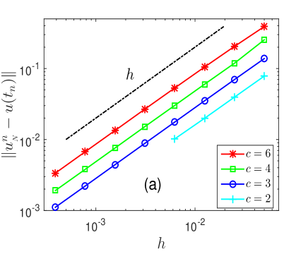
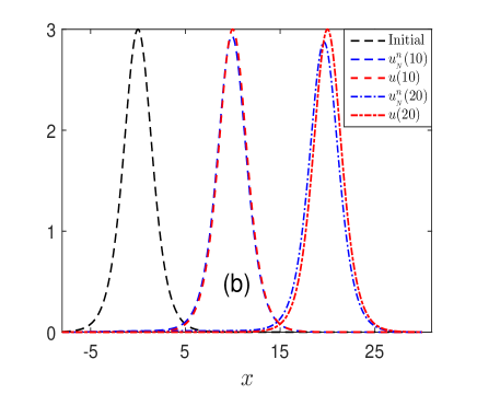
Figure 1: Numerical simulation for the solitary-wave solution (4.1). (a) The error of the first-order scheme (2.4) at $T=2$ for various choices of $h$ and $c$. The time step size $\tau$ satisfies $\tau=h/c$. The broken line has slope one. (b) The numerical solution at $T=10,20$ was obtained by the scheme (2.4) with $h=1/200$ and $\tau=h/4$.

Example 2. The initial data of the KdV equation (1.1) is now chosen as

$$u_{0}(x)=3\,{\mathrm{sech}}^{2}(2x)\sin(x),\qquad x\in[-\pi,\pi].$$ (4.2)

The initial data and the numerical solution for $T=3$ with $c=3$, $h=\pi/2^{11}$ and $\tau=h/\pi$ are displayed in Figure 2 (b), where the reference solution is obtained by the second-order exponential integrator of [16] with $\tau=10^{-6}$ and $h=\pi/2^{15}$. The error of the scheme (2.4) with $c=3$ and $\tau=h/\pi$ is shown in Figure 2 (a). The graph clearly shows first-order convergence of the scheme (2.4).

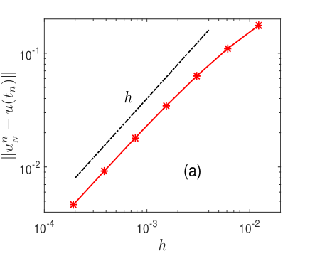
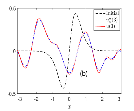
Figure 2: Numerical simulation for the initial value (4.2). (a) The error of the first-order scheme (2.4) at $T=3$ for various choices of $h$ with $c=3$ and $\tau=h/\pi$. The broken line has slope one. (b) The numerical solution at $T=3$ was computed with the scheme (2.4) using $h=\pi/2^{11}$ and $\tau=h/\pi$.

References

• [1] E. Aksan and A. Özdeş, Numerical solution of Korteweg–de Vries equation by Galerkin B-spline finite element method, Appl. Math. Comput., 175 (2006), pp. 1256–1265.
• [2] D. N. Arnold and R. Winther, A superconvergent finite element method for the Korteweg–de Vries equation, Math. Comput., 38 (1982), pp. 23–36.
• [3] W. Bao, X. Dong and X. Zhao, An exponential wave integrator sine pseudospectral method for the Klein–Gordon–Zakharov system, SIAM J. Sci. Comput., 35 (2013), pp. A2903–A2927.
• [4] J. Bourgain, Fourier transform restriction phenomena for certain lattice subsets and applications to nonlinear evolution equations, Geom. Funct. Anal., 3 (1993), pp. 209–262.
• [5] T. Chan and T. Kerkhoven, Fourier methods with extended stability intervals for the Korteweg–de Vries equation, SIAM J. Numer. Anal., 22 (1985), pp. 441–454.
• [6] J. Colliander, M. Keel, G. Staffilani, H. Takaoka and T. Tao, Sharp global well-posedness for KdV and modified KdV on $\mathbb{R}$ and $\mathbb{T}$, J. Amer. Math. Soc., 16 (2003), pp. 705–749.
• [7] C. Courtès, F. Lagoutière and F. Rousset, Numerical analysis with error estimates for the Korteweg–de Vries equation, arXiv:1712.02291, (2017).
• [8] G. Das and J. Sarma, A new mathematical approach for finding the solitary waves in dusty plasma, Phys. Plasmas, 5 (1998), pp. 3918–3923.
• [9] R. Dutta, U. Koley and N. H. Risebro, Convergence of a higher order scheme for the Korteweg–de Vries equation, SIAM J. Numer. Anal., 53 (2015), pp. 1963–1983.
• [10] L. Einkemmer and A. Ostermann, A split step Fourier/discontinuous Galerkin scheme for the Kadomtsev–Petviashvili equation, Appl. Math. Comput., 334 (2018 ), pp. 311–325.
• [11] K. Goda, On stability of some finite difference schemes for the Korteweg–de Vries equation, J. Phys. Society Japan, 39 (1975), pp. 229–236.
• [12] M. Gubinelli, Rough solutions for the periodic Korteweg–de Vries equation, Comm. Pure Appl. Anal., 11 (2012), pp. 709–733.
• [13] M. Helal and M. Mehanna, A comparative study between two different methods for solving the general Korteweg–de Vries equation (GKdV), Chaos, Solitons & Fractals, 33 (2007), pp. 725–739.
• [14] M. Hochbruck and A. Ostermann, Explicit exponential Runge–Kutta methods for semilinear parabolic problems, SIAM J. Numer. Anal., 43 (2005), pp. 1069–1090.
• [15] M. Hochbruck and A. Ostermann, Exponential integrators, Acta Numer., 19 (2010), pp. 209–286.
• [16] M. Hofmanová and K. Schratz, An exponential-type integrator for the KdV equation, Numer. Math., 136 (2017), pp. 1117–1137.
• [17] H. Holden, K. Karlsen, N. Risebro, and T. Tao, Operator splitting for the KdV equation, Math. Comput., 80 (2011), pp. 821–846.
• [18] H. Holden, K. H. Karlsen, and N. H. Risebro, Operator splitting methods for generalized Korteweg–de Vries equations, J. Comput. Phys., 153 (1999), pp. 203–222.
• [19] H. Holden, U. Koley, and N. Risebro, Convergence of a fully discrete finite difference scheme for the Korteweg–de Vries equation, IMA J. Numer. Anal., 35 (2015), pp. 1047–1077.
• [20] H. Holden, C. Lubich, and N. Risebro, Operator splitting for partial differential equations with Burgers nonlinearity, Math. Comput., 82 (2013), pp. 173–185.
• [21] C. Klein, Fourth order time–stepping for low dispersion Korteweg–de Vries and nonlinear Schrödinger equation, Electron. Trans. Numer. Anal., 29 (2008), pp. 116–135.
• [22] C. Klein and K. Roidot, Fourth order time-stepping for Kadomtsev–Petviashvili and Davey–Stewartson equations, SIAM J. Sci. Comput., 33 (2011), pp. 3333–3356.
• [23] D. Korteweg and G. de Vries, On the change of form of long waves advancing in a rectangular channel, and a new type of long stationary wave, Phil. Mag., 39 (1895), pp. 422–443.
• [24] J. D. Lawson, Generalized Runge–Kutta processes for stable systems with large Lipschitz constants, SIAM J. Numer. Anal., 4 (1967), pp. 372–380.
• [25] H. Ma and B. Guo, The Fourier pseudospectral method with a restrain operator for the Korteweg–de Vries equation, J. Comput. Phys., 65 (1986), pp. 120–137.
• [26] H. Ma and W. Sun, A Legendre–Petrov–Galerkin and Chebyshev collocation method for third-order differential equations, SIAM J. Numer. Anal., 38 (2000), pp. 1425–1438.
• [27]  , Optimal error estimates of the Legendre–Petrov–Galerkin method for the Korteweg–de Vries equation, SIAM J. Numer. Anal., 39 (2001), pp. 1380–1394.
• [28] Y. Maday and A. Quarteroni, Error analysis for spectral approximation of the Korteweg–de Vries equation, ESAIM: Math. Model. Numer. Anal., 22 (1988), pp. 499–529.
• [29] A. Osborne, The inverse scattering transform: tools for the nonlinear Fourier analysis and filtering of ocean surface waves, Chaos, Solitons & Fractals, 5 (1995), pp. 2623–2637.
• [30] L. Ostrovsky and Y. A. Stepanyants, Do internal solitions exist in the ocean?, Rev. Geophys., 27 (1989), pp. 293–310.
• [31] A. Rashid, Convergence analysis of three-level Fourier pseudospectral method for Korteweg–de Vries Burgers equation, Comput. Math. Appl., 52 (2006), pp. 769–778.
• [32]  , Numerical solution of Korteweg–de Vries equation by the Fourier pseudospectral method, Bull. Belg. Math. Soc., 14 (2007), pp. 709–721.
• [33] A. Rashid, T. Mahmood, and G. Mustafa, An explicit pseudospectral scheme for Korteweg–de Vries Burgers equation, Inter. J. Pure Appl. Math., 16 (2004), pp. 439–449.
• [34] J. Shen, A new dual-Petrov-Galerkin method for third and higher odd-order differential equations: application to the KdV equation, SIAM J. Numer. Anal., 41 (2003), pp. 1595–1619.
• [35] J. Shen, T. Tang, and L.-L. Wang, Spectral methods: algorithms, analysis and applications, Springer, Berlin, Heidelberg, 2011.
• [36] T. R. Taha and M. I. Ablowitz, Analytical and numerical aspects of certain nonlinear evolution equations. III. Numerical, Korteweg–de Vries equation, J. Comput. Phys., 55 (1984), pp. 231–253.
• [37] J. A. Trangenstein, Numerical solution of hyperbolic partial differential equations, Cambridge University Press, 2009.
• [38] A. Vliegenthart, On finite–difference methods for the Korteweg–de Vries equation, J. Eng. Math., 5 (1971), pp. 137–155.
• [39] R. Winther, A conservative finite element method for the Korteweg–de Vries equation, Math. Comput., (1980), pp. 23–43.