Non-linear Breit-Wheeler process in short laser double-pulses

Abstract

The non-linear (strong-field) Breit-Wheeler $e^{+}e^{-}$ pair production by a probe photon traversing two consecutive short and ultra short (sub-cycle) laser pulses is considered within a QED framework. The temporal shape of the pulses and the distance between them are essential for the differential cross section as a function of the azimuthal angle distribution of the outgoing electron (positron). The found effect of a pronounced azimuthal anisotropy is important for sub-cycle pulses and decreases rapidly with increasing width of the individual pulses.

I Introduction

The rapidly progressing laser technology Tajima offers novel and unprecedented opportunities to investigate quantum systems with intense laser beams Piazza . An intensity $I_{L}$ of $\sim 2\times 10^{22}$ W/cm² has been already achieved I-22 . Intensities of the order of $I_{L}\sim 10^{23}...10^{25}$ W/cm² are envisaged in the near future, e.g. at CLF CLF , ELI ELI , or HiPER hiper . Further facilities are in the planning or construction stages, e.g. the PEARL laser facility sarov at Sarov/Nizhny Novgorod, Russia. The high intensities are provided in short pulses on a femtosecond pulse duration level Piazza ; ShortPulse ; ShortPulse_2 , with only a few oscillations of the electromagnetic (e.m.) field or even sub-cycle pulses. (The tight connection of high intensity and short pulse duration is further emphasized in Mackenroth-2011 . The attosecond regime will become accessible at shorter wavelengths atto ; I-222 ).

New laser facilities may utilize short and ultra-short pulses in ”one-” or ”few-” cycle regimes. In this case, a determination of the pulse fine-structure is very important and, in particular, tasking the phase difference between the electric field and pulse envelope, i. e. the carrier envelope phase (CEP). It was found that the CEP effect is especially important just for the case of the short and ultra-short (sub-cycle) pulses (cf. CEPTitov and references therein; for recent access option for the CEP in long pulses, cf. Li:2018xnp ).

The study of quantum processes in two consecutive (or double) laser pulses with taking into account CEP effect is a new important and interesting topic in laser physics. An analysis of Breit-Wheeler pair production within the framework of scalar electrodynamics is provided in JansenMuller . Below, we give a further development of this problem. We extend that previous consideration to QED, where $e^{+}e^{-}$ are fermions, and we concentrate our attention on the azimuthal angle distribution of outgoing electron (positron) at fixed CEP. In fact, the non-linear Breit-Wheeler process considered below, assumes the interaction of a probe photon $X$ (e.g. from Compton backscattering in a pre-pulse, starting a seeded cascade via two-step part of trident process, cf. Blackburn:2017dpn ; Blackburn:2018ghi ) with two consecutive laser pulses, $L_{1+2}$, in the reaction $X+L_{1+2}\to e^{+}+e^{-}$, where a multitude of laser photons can participate simultaneously in the $e^{+}e^{-}$ pair creation, thus enabling the process even ”below threshold”. In the Furry picture, this process is a cross channel of the non-linear Compton process without having a classical counterpart, as the Thomson process in the weal-field regime. The non-linear Breit-Wheeler process means the decay of the probe photon into a laser-dressed electron ($e^{-}$) positron ($e^{+}$) pair. The emphasis here is on short and intense laser pulses. Long and weak laser pulses are dealt with in the standard textbook Breit-Wheeler process (cf. the review paper Ritus-79 ). Various aspects, such as the impact of the pulse envelope, pulse duration, pulse polarization, of $e^{+}e^{-}$ pair creation in single pulses were analyzed, e.g. in Refs. TitovPEPAN ; TitovPRA ; TitovPRL ; Nousch ; Krajewska with special emphasis on CEP effects A1 ; CEPTitov , spin effects Jansen:2016gvt , bi-frequent pulses Jansen:2013dea ; Nousch:2015pja ; Otto:2016fdo , spectral caustics Nousch:2015pja , and focusing effects DiPiazza:2016maj ; DiPiazza:2016tdf .

One may contrast the single-pulse laser beams to a long train of pulses or multi-pulses, where a special modulation of the phase space distribution of produced $e^{\pm}$ in comb structures arises due to interference effect Krajewska:2014ssa . In some sense, such a situation refers to multi-shot experiments, where a laser with extremely high repetition rate fires for some time. (Another option is the pulse train generation at XFELs, cf. Decker .) In between is the presently considered case of a double pulse. Below, we concentrate mainly on the interplay of the effect of CEP and the shape of the laser beams which is determined by the temporal shape of the individual pulses (cf. TitovPRA ) and the separation distance between them.

Our present paper is a follow-up of CEPTitov which is inspired by JansenMuller . Differences are (i) Fermion pairs (JansenMuller deals with Bose pairs), (ii) circular polarization (JansenMuller uses linear polarization), (iii) many details of the laser pulse modeling (JansenMuller uses separate individual pulses with particular envelope functions, while our field arises from ”cutting out” the pulses by a double hump window function with hump separation $\geq 0$), (iv) consideration of very short and sub-cycle pulses, (v) focus on sub-threshold pair production, (vi) focus on azimuthal angle distribution (JansenMuller considers the energy spectra).

Our paper is organized as follows. In Sect. II, the double-pulse field model is presented. Sect. III recalls the basic expressions for the relevant observables in non-linear Breit-Wheeler $e^{+}e^{-}$ pair production. In Sect. IV we discuss results of numerical calculations. Our summary is given in Sect. V.

II Model of the double pulse

In the following we use the electromagnetic (e.m.) four-potential for a circularly polarized laser field in the axial gauge $A^{\mu}=(0,\,\mathbf{A}(\phi))$ with

$$\mathbf{A}(\phi)=f(\phi)\left(\mathbf{a}_{1}\cos(\phi+\tilde{\phi})+\mathbf{a}_{2}\sin(\phi+\tilde{\phi})\right)~{},$$ (1)

where $\tilde{\phi}$ is the CEP. The quantity $\phi=k\cdot x$ is the invariant phase with four-wave vector $k=(\omega,\mathbf{k})$, obeying the null field property $k^{2}=k\cdot k=0$ (a dot between four-vectors indicates the Lorentz scalar product) implying $\omega=|\mathbf{k}|$, $\mathbf{a}_{(1,2)}\equiv\mathbf{a}_{(x,y)}$; $|\mathbf{a}_{x}|^{2}=|\mathbf{a}_{y}|^{2}=a^{2}$, $\mathbf{a}_{x}\mathbf{a}_{y}=0$; transversality means $\mathbf{k}\mathbf{a}_{x,y}=0$ in the present gauge. The envelope function $f(\phi)$ in case of two consecutive pulses is chosen as sum of two hyperbolic secants

$$f(\phi)=\frac{1}{\cosh(\frac{\phi}{\Delta}-G)}+\frac{1}{\cosh(\frac{\phi}{\Delta}+G)},$$ (2)

where $G$ is the separation parameter of two consecutive short pulses which is equal to the distance between the centers of the two consecutive pulses. The dimensionless quantity $\Delta$ is related to the single pulse duration $2\Delta=2\pi N$, where $N$ has the meaning of a number of cycles in the individual pulse. It is related to the time duration of the pulse $\tau=2N/\omega$.

One may imagine the generation of the above described pulse structures by the sequence of a laser beam - beam splitter - a delay section for one of the split beams and subsequently the merging of both beams. Presently, the alignment of two separate laser beams of seems hardly possible to be realized with equal carrier envelope phases and precisely adjustable temporal pulse delay together with keeping constant the polarizations. In this respect, our field model (1, 2) is highly idealized, but enjoys a minimum number of parameters. However, having in mind principle effects of quantum interference patterns by such double-slit phenomena in the temporal domain, our field model can be regarded as useful representative ansatz. For further discussion of aspects of double-and multi-slit phenomena we refer the interested reader to JansenMuller with references quoted therein.

For an illustration, in Fig. 1 we show the $x$ component of the e.m. potential $A_{x}/a$ as a function of invariant phase $\phi$ for different values of the separation parameter $G$. The case $G=0$ corresponds to the complete overlap of the two envelopes which leads to the e.m. potential with a double amplitude $a$.

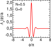
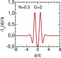
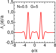
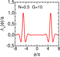
Figure 1: (Color online) The e.m. potential $A_{x}/a$ in Eq. (2) as a function of the invariant phase $\phi=k\cdot x$ for sub-cycle pulse with $N=1/2$ and different values of the separation parameter $G=0,\,2,\,5,\,10$ as it is indicated in the legends.

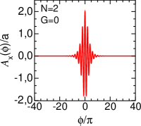
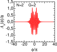
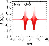
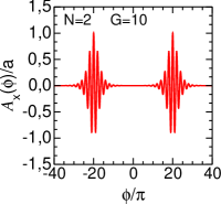
Figure 2: (Color online) The same as in Fig. 1 but for a short pulse with $N=2$.

The e.m. potential $A_{x}/a$ for a short pulse with $N=2$ and different $G$ is exhibited in Fig. 2.

As mentioned above, the interplay between carrier envelope phase $\tilde{\phi}$ and separation parameter $G$ is the main subject of our present discussion and, as we will show, it has a strong impact on the azimuthal angle distribution of the outgoing electron (positron), in particular for a short pulse duration $\Delta$. We will consider essentially multi-photon events, where a finite number of laser photons is involved into the $e^{+}e^{-}$ pair production. This allows for the sub-threshold $e^{+}e^{-}$ pair production with $s<s_{\rm thr}$, where $s=(k_{x}+k)^{2}$ is the square of total energy in the center of mass system (c.m.s., defined by $\mathbf{k}_{x}=-\mathbf{k}$, $s_{c.m.s.}=4\omega_{X}\omega$), $s_{\rm thr}=4m^{2}$ is it threshold value, where $m$ is the electron mass. We also discuss dependence of the cross section on e.m. field intensity which is described by the reduced field intensity $\xi^{2}=e^{2}a^{2}/m^{2}$. We use natural units with $c=\hbar=1$, $e^{2}/4\pi=\alpha\approx 1/137.036$.

III Cross section and anisotropy

The azimuthal angular differential cross can be cast into the form (cf. Appendix A for details)

$$\frac{d\sigma}{d\phi_{e^{+}}}=\frac{\alpha^{2}\,\zeta}{4m^{2}\xi^{2}N_{0}}\,\int\limits_{\zeta}^{\infty}\,d\ell\,v(\ell)\,\int\limits_{-1}^{1}d\cos\theta_{e^{+}}\,w{(\ell)}~{}$$ (3)

with partial probabilities

$$w(\ell) = 2|\widetilde{Y}_{\ell}(z)|^{2}+\xi^{2}(2u-1)$$

$$\times \left(|Y_{\ell-1}(z)|^{2}+|Y_{\ell+1}(z)|^{2}-2{\rm Re}\,(\widetilde{Y}_{\ell}(z)X^{*}_{\ell}(z))\right),$$

which recover the known expressions Ritus-79 in case of infinitely long e.m. pulses, where $\ell$ becomes a discrete (integer) variable (cf. CEPTitov ). The azimuthal angle of the outgoing positron, $\phi_{e^{+}}$, is defined as $\cos\phi_{e^{+}}={\mathbf{a}_{x}}{\mathbf{p}}_{e^{+}}/a|{\mathbf{p}}_{e^{+}}|$. It is related to the azimuthal angle of the electron by $\phi_{e}=\phi_{e^{+}}-\pi$. Furthermore, $\theta_{e^{+}}$ is the polar angle of outgoing positron, $v$ is the positron (electron) velocity in c.m.s.. The averaging and sum over the spin variables in the initial and the final states is executed.

The lower limit of the integral over the variable $\ell$ is the threshold parameter $\zeta=s_{\rm thr}/s\equiv 4m^{2}/s$. The region of $\zeta<1$ corresponds to the above-threshold $e^{+}e^{-}$ pair production, while the region of $\zeta>1$ matches the sub-threshold pair production. We keep our notation of CEPTitov and denote four-vectors $k(\omega,{\mathbf{k}})$, $k^{\prime}(\omega^{\prime},{\mathbf{k}}^{\prime})\equiv k_{x}(\omega_{x},{\mathbf{k}}_{x})$, $p(E,{\mathbf{p}})$ and $p^{\prime}(E^{\prime},{\mathbf{p}}^{\prime})$ as the four-momenta of the background (laser) field (1), incoming probe photon, outgoing positron and electron, respectively. The variables $s$, $v$ and $u$ are determined by $s={2k\cdot k^{\prime}}=2(\omega^{\prime}\omega-{\mathbf{k}}^{\prime}{\mathbf{k}})$ (with $\mathbf{k}^{\prime}\mathbf{k}=-\omega^{\prime}\omega$ for head-on geometry), $v^{2}=(\ell s-4m^{2})/\ell s$, $u\equiv(k^{\prime}\cdot k)^{2}/\left(4(k\cdot p)(k\cdot p^{\prime})\right)=1/(1-v^{2}\cos^{2}\theta_{e})$. The factor $N_{0}$ reads $N_{0}={1}/{2\pi}\int_{-\infty}^{\infty}d\phi\,(f^{2}(\phi)+{f^{\prime}}^{2}(\phi))$ and normalizes to the photon flux in case of finite pulses TitovEPJD . The variable $\ell$ takes continuous values and the product $\ell\omega$ has the meaning of the laser energy involved in the process (see also A1 for a recent discussion).

The basic functions $Y_{\ell}$ and $X_{\ell}$ entering partial probabilities (III) the may be considered as generalized Bessel functions for the finite e.m. pulse,

$$Y_{\ell}(z) = \frac{1}{2\pi}{\rm e}^{-i\ell(\phi_{0}-\tilde{\phi})}\int\limits_{-\infty}^{\infty}\,d\phi\,{f}(\phi)\,{\rm e}^{i\ell\phi-i{\cal P}(\phi)}~{},$$ (5)

$$X_{\ell}(z) = \frac{1}{2\pi}{\rm e}^{-i\ell(\phi_{0}-\tilde{\phi})}\int\limits_{-\infty}^{\infty}\,d\phi\,{f^{2}}(\phi)\,{\rm e}^{i{\ell}\phi-i{\cal P}(\phi)},$$ (6)

$$\widetilde{Y}_{\ell}(z) = \frac{z}{2\ell}\left(Y_{\ell+1}(z)+Y_{\ell-1}(z)\right)-\xi^{2}\frac{u}{u_{\ell}}\,X_{\ell}(z)$$ (7)

with the phase function

$${\cal P(\phi)} = z\int\limits_{-\infty}^{\phi}\,d\phi^{\prime}\,\cos(\phi^{\prime}-\phi_{0}+\tilde{\phi})f(\phi^{\prime})$$ (8)

$$- \xi^{2}\zeta u\int\limits_{-\infty}^{\phi}\,d\phi^{\prime}\,f^{2}(\phi^{\prime})~{},$$

where $\phi_{0}$ is the azimuthal angle of the outgoing electron $\phi_{0}\equiv\phi_{e}=\phi_{e+}-\pi$ and the argument $z$ of the generalized Bessel functions is related to $\xi$, $\ell$ and $u$ via $z=2{\ell}\xi\sqrt{{u}/{u_{\ell}}\left(1-{u}/{u_{\ell}}\right)}$ with $u_{\ell}\equiv\ell/\zeta$.

Together with the differential cross section $d\sigma/d\phi_{e}$ we analyze the anisotropy of the electron (positron) emission as a function as a function of the positron (electron) azimuthal angle

$${\cal A}=\frac{{d\sigma(\phi_{e})}-{d\sigma(\phi_{e^{+}})}}{{d\sigma(\phi_{e})}+{d\sigma(\phi_{e^{+}})}}.$$ (9)

The cross section (3) and anisotropy (9) have a non-trivial, non-monotonic dependence as a function of azimuthal angle $\phi_{e^{+}}$ $(\phi_{e})$, which is determined by the values of the carrier phase $\tilde{\phi}$ and separation parameter $G$. On a qualitative level, the reason for such behavior is the following. The basic functions $Y_{\ell}$ and $X_{\ell}$ are determined by the integral over $d\phi$ with a rapidly oscillating exponential function $\exp[i\Psi]$ with leading terms

$$\Psi=\ell\phi - z\Delta\cos(\Phi-G\Delta)\int\limits_{-\infty}^{\frac{\phi}{\Delta}-G}dt\,f_{0}(t)\cos(t\Delta)$$ (10)

$$- z\Delta\sin(\Phi-G\Delta)\int\limits_{-\infty}^{\frac{\phi}{\Delta}-G}dt\,f_{0}(t)\sin(t\Delta)$$

$$- z\Delta\cos(\Phi+G\Delta)\int\limits_{-\infty}^{\frac{\phi}{\Delta}+G}dt\,f_{0}(t)\cos(t\Delta)$$

$$- z\Delta\sin(\Phi+G\Delta)\int\limits_{-\infty}^{\frac{\phi}{\Delta}+G}dt\,f_{0}(t)\sin(t\Delta)~{},$$

$$+ \cdots$$

where $f_{0}(t)=1/\cosh(t)$ and $\Phi=\phi_{e}-\tilde{\phi}$. The ellipses refer to contributions from the second line in (8). Due to the fact that for short (ultra-short) pulses

$$\int\limits_{-\infty}^{t}dt^{\prime}\,f_{0}(t^{\prime})\cos(t^{\prime}\Delta)\gg\int\limits_{-\infty}^{t}dt^{\prime}\,f_{0}(t^{\prime})\sin(t^{\prime}\Delta)~{},$$ (11)

one can conclude that the maximum value to the highly oscillating integrals determined the basic functions $Y_{\ell}$ and $X_{\ell}$ comes from the range $\Phi\pm G\Delta\simeq 2n\pi$, where $n$ is an integer $n=0,\,1,\,2\,\cdots$. Then the differential cross section would be enhanced at

$$\phi^{\rm max}_{e^{+}}-\tilde{\phi}=(2n+1)\pi\pm G\Delta~{}.$$ (12)

IV Numerical results

IV.1 Azimuthal distributions

Let us consider first the sub-cycle pulse with $N=1/2$, i.e. $\Delta=\pi/2$. For sub-cycle pulses, the electric field field vector does not rotate in the $\mathbf{k}$-transverse plane with full length. This asymmetry, which is also seen in Fig. 1 as strong asymmetry in the $\pm A_{x}$ directions, leaves such a strong imprint on the azimuthal distribution of $e^{\pm}$. It rapidly disappears for longer pulses, i.e. larger values of $N$, as already evidenced by Fig. 2.

To be specific we consider the differential cross section $d\sigma/d\phi_{e^{+}}$ for sub-cycle pulse with $N=1/2$ as a function of azimuthal angle of positron momentum at different values of separation parameter $G$ and fixed CEP $\tilde{\phi}=0$ exhibited in the left panel of Fig. 3. One can see the oscillating structure of the cross section. The positions of the maxima and the frequencies of the oscillations depend on the separation parameter.

The dependence of the differential cross section for ultra-short pulse on CEP at fixed separation parameter $G=8$ is expressed in the right panel of Fig. 3 One can see that the cross sections have a bump-like structure and, besides, the bump positions coincide with the corresponding carrier phases. If one plots the cross sections as a function of the useful ”scale variable”

$$\chi_{e^{+}}=\phi_{e^{+}}-\tilde{\phi}$$ (13)

then the all curves expressed in right panel of Fig. 3 merge into one (that is the blue one labeled by $\tilde{\phi}=0$). The entire dependence the differential cross section on ˜$\tilde{\phi}$ is contained in the variable $\chi_{e^{+}}$ (cf. CEPTitov ). Later we use this variable in our discussion.

According to (14) the differential cross section would be enhanced at

$$\chi_{e^{+}}=\phi^{\rm max}_{e^{+}}-\tilde{\phi}=(2n+1)\pi\pm G\Delta$$ (14)

This is in pretty good agreement with results of our full calculation shown in the left panel of Fig. 3 (recollect that in this calculation $\tilde{\phi}=0$). Thus, for pulse separation $G=4$ choice for integer $n=0,\,-1$ leads to the bump position $\phi_{e^{+}}=\pi+(\pm\,2\pi)$ and $-\pi+(\pm\,2\pi)$. This is coincides with results exhibited in the right panel of Fig. 3, since the phase factor $(\pm\,2\pi)$ may be omitted. Similar results one can obtained for separation parameters $G=10$ with $\phi_{e^{+}}^{max}=0,\pm\,2\pi$ and $G=5$ with $\phi_{e^{+}}^{max}=\pm\,\pi/2\,\pm\,3\pi/2$, respectively.

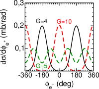
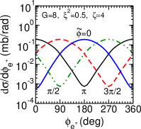
Figure 3: (Color online) Differential cross section $d\sigma/d\phi_{e^{+}}$ of Eq. (3) for various values of the separation parameter $G$ and the carrier envelope phase $\tilde{\phi}$. For $N=1/2$, $\xi^{2}=0.5$ and $\zeta=4$. Left panel: $G=4$ (sold black curve), 5 (dashed green curve) and 10 (dashed red curve); $\tilde{\phi}=0$. Right panel: $G=8$ and $\tilde{\phi}=0$ (solid blue curve), $\pi/2$ (dot-dashed green curve), $\pi$ solid black curve), $3\pi/2$ ( dashed red curve). When plotting the curves as a function of $\chi_{e^{+}}=\phi_{e^{+}}-\tilde{\phi}$ they coincide with the blue curve labeled by $\tilde{\phi}=0$.

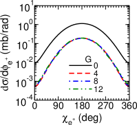
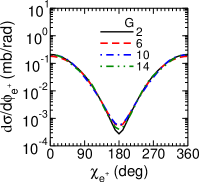
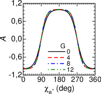
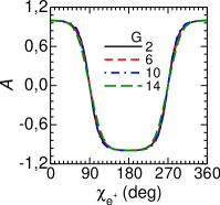
Figure 4: (Color online) Top panels : The differential cross section of Eq. (3) as a function of $\chi_{e^{+}}$ for $N=1/2$, pulses separation parameter $G=0,4,8,12$ and $G=2,6,10,14$ shown in the left and right panels, respectively. Bottom panels : The same as in the top panels, but for the anisotropy of Eq. (9).

Let us now focus on the dependence of the azimuthal angular distribution on the separation parameter $G$, again for sub-cycle pulse with $N=1/2$. At $G=4n$, the cross section of $e^{+}e^{-}$ production is expected to be enhanced at

$$\chi_{e^{+}}=(2n+1)\pi~{}.$$ (15)

The corresponding cross sections and anisotropies as a function of $\chi_{e^{+}}$ calculated numerically using Eqs. (3) and (9, respectively are displayed in the top and bottom parts of the right panels in Fig. 4. One can see sharp bumps in the cross sections and anisotropies at $\chi_{e}^{+}=\pi$, which coincide with our qualitative prediction (15).

The case $G=0$ is exceptional, since the two pulses completely overlap and the cross section is greatly enhanced. The main reason of such enhancement is related to the modification of highly oscillating function $\Psi$ in Eq. (10). Now, the leading term reads

$$\Psi\simeq\ell\phi - 2z\Delta\cos(\Phi)\int\limits_{-\infty}^{\frac{\phi}{\Delta}}dt\,f_{0}(t)\cos(t\Delta)$$ (16)

$$- 2z\Delta\sin(\Phi)\int\limits_{-\infty}^{\frac{\phi}{\Delta}}dt\,f_{0}(t)\sin(t\Delta),$$

which leads to renormalization $z\to 2z$ or $\xi^{2}\to 4\xi^{2}$. The cross section increases with $\xi^{2}$ see, for example TitovPEPAN ) and our next section therefore one can see strong enhancement of the cross section at $G=0$.

The situation changes dramatically for the separation parameter $G=2+4n$. In this case, the cross sections and anisotropies are enhanced at $\phi_{e^{+}}-\tilde{\phi}=0$ and $2\pi$ as illustrated in the right panels of Fig. 4. Here, we face also some (approximate) symmetry: the right column curves are generated by shifting $\chi_{e^{+}}\to\chi_{e^{+}}\pm\pi$.

Both examples show the explicit correlation between separation parameter $G$ and the carrier phase $\tilde{\phi}$ in the different cross section $d\sigma/d\phi_{e^{+}}$, especially for $G<2$. For larger values of $G$, the cross section becomes independent of the separation parameter $G$.

A similar behavior is expected for wider pulses. For instance, in Fig. 5 we display results for the short pulse with $N=1$ corresponding to $\Delta=\pi$. Using Eq. (15) one can find that the bump-like structure with the bump position $\chi_{e^{+}}=\pi$ appears at $G=2n$, as confirmed by our full numerical calculation exhibited in the left panels of Fig. 5. The values of the separation parameter $G=2n+1$ result in an enhancement of the cross section and anisotropies at $\chi_{e^{+}}=0$ and $2\pi$ (cf. right panels of Fig. 5).

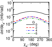
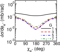
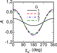
Figure 5: (Color online) The same as in Fig. 4 but for $N=1$ and pulses separation parameter $G=0,2,4,6$ and $G=1,3,5,7$ shown in the left and right panels, respectively.

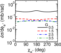
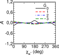
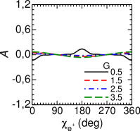
Figure 6: (Color online) The same as in Fig. 4 but for $N=2$ and separation parameter $G=0,1,2,3$ and $G=1/2,3/2,5/2,7/2$ shown in the left and right panels, respectively.

For wider pulses with $N\geq 2$ the bump structure and the non-monotonic behavior becomes very weak. For example, Fig. 6 illustrates our result for the short pulses with $N=2$, that is $\Delta=2\pi$.

Nevertheless, some enhancement (weak bump structure at $\phi_{e^{+}}-\tilde{\phi}=\pi$) is expected at $G=0,\,1,\,2,\,\cdots$, while the enhancement at $\phi_{e}=0$ and $2\pi$ is expected at half-integer values $G=1/2,\,3/2,\,5/2,\,\cdots$. Our corresponding result is depicted in Fig. 6. Our full numerical calculation does not support the qualitative prediction of (10).

IV.2 Total cross section

With the given parameterization (1, 2), the total cross section depends on the available energy $s$ (encoded in the sub-threshold parameter $\zeta$), the laser intensity parameter $\xi$, the double-pulse distance parameter $G$, and the cycle number $N$ (encoded in the pulse width parameter $\Delta$): $\sigma(s;\xi^{2},G,N)$ since the CEP dependence disappears. A few of these dependencies are now considered. For simplicity and without loss of generality below we consider sub-cycle and short pulses with $N=1/2$ and $N=1$, respectively. Our analysis shows that wilder pulses do not bring new qualitative results.

The dependence of the total cross section as a function of the field intensity $\xi^{2}$ is exhibited in Fig. 7. We choose sub-threshold pulse with $N=0.5$ and the separation parameter $G=4n$ according to Fig. 4, left panels. One can see that all curves coincide with another at $G\geq 2$, where the dependence on the separation parameter disappears. Qualitatively, the behavior of the cross sections shown in the left and right panels are similar, being enhanced for sub-cycle pulse, especially for small vales of $\xi^{2}$.

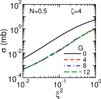
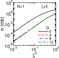
Figure 7: (Color online) The total cross section of the $e^{+}e^{-}$ production as a function of the reduced field intensity $\xi^{2}$. The results are for $N=1/2$, sub-threshold parameter $\zeta=4$ and various values of the separation parameter $G$ listed in the legend.

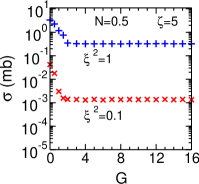
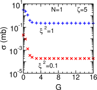
Figure 8: (Color online) The total cross section of the $e^{+}e^{-}$ production as a function of separation parameter $G$ at $\xi^{2}=0.1$ and $\xi^{2}=1$, and $\zeta=5$. Left and right panels correspond to $N=1/2$ and $N=1$, respectively.

This is correlated with results shown in Fig. 8, where the total cross sections as a function of the separation parameter $G$ for the sub-cycle ($N=1/2$) and short ($N=1$) pules are shown in the left and right panels, respectively. The calculations are for the sub-threshold parameter $\zeta=5$ and the field intensities $\xi^{2}=0.1$ and $1$. The cross sections for $\xi^{2}=1$ are much greater compared to the case of $\xi^{2}=0.1$. One can see a significant enhancement of the cross sections at $G<2$ which is a consequence of strong overlap of the two pulses, discussed above, cf. top in Figs. 4 and 5. The cross sections at $G\geq 2$ are independent of $G$ and exhibit some plateau. For the sub-cycle pulses at chosen parameters within the accuracy of our calculation, the cross sections at the plateau are $\approx 1.4\times 10^{-3}$ mb and $\approx 0.32$ mb for $\xi^{2}=0.1$ and $1$, respectively. For the short pulses ($N=1$), the result is qualitatively similar to that shown in the left panel but the cross sections are smaller compared to the case of $N=1/2$. Thus, the cross sections at plateau are $\approx 1.9\times 10^{-4}$ mb and $\approx 0.22$ mb for $\xi^{2}=0.1$ and $1$, respectively. The enhancement of the cross sections for the sub-cycle pulses compared to the short pulses, especially for small $\xi^{2}$, is consistent with our results exhibited in Fig. 7 and below in Fig. 9. Note that the results displayed in Figs. 7 and 8 are obtained at different values of the subthreshold parameter $\zeta=4$ and $5$, respectively.

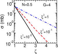
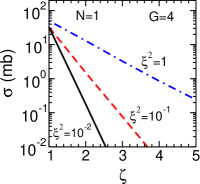
Figure 9: (Color online) The total cross section of the $e^{+}e^{-}$ production as a function of sub-threshold parameter $\zeta$ for various $\xi^{2}$ at fixed $G=4$ and $N=1/2$.

The total cross section as a function of the sub-threshold parameter $\zeta$ is exhibited in Fig. 9 for different values of field intensity $\xi^{2}$ and $G=4$. The left and right panels correspond to $N=1/2$ and $N=1$, respectively. One can see an almost exponential decrease of the cross section with $\zeta$. The slope of the curves decreases with increasing intensity of the electromagnetic field (or $\xi^{2}$). (Closer inspection shows that this result does not depend on the separation parameter $G\geq 2$ which is correlated with results exhibited in Fig. 8.) Qualitatively, results for sub-cycle and short pulses are similar. The curves in case of sub-cycle pulses are slightly flatter.

V summary

In summary we have analyzed the non-linear (strong-field) Breit-Wheeler $e^{+}e^{-}$ production in case of two consecutive circularly polarized short pulses with equal carrier phases. We find that for short pulses with the number of oscillation in the pulse $N\leq 1$ the azimuthal angular differential cross section is sensitive to both the carrier phase $\tilde{\phi}$ and the separation parameter $G$. That is manifest in the bump-like behavior of the differential cross section. Results of the full numerical calculations coincide with simple analytical expressions. This means that the azimuthal angle distribution of outgoing fermions may be used as a powerful method for determination of the structure of the short double pulses (or the carrier phase at the fixed pulse geometry).

The total cross section obeys a monotonic (near-exponential) increase with the field intensity $\xi^{2}$ at fixed sub-threshold parameter $\zeta$ and an exponential decrease of cross section with increasing $\zeta$ at fixed $\xi^{2}$. The total cross sections increases significantly for $G<2$ because of strong interference in case of overlapping pulses. All these facts can be used in planning appropriate experiments.

Appendix A Evaluation of the partial probability $\mathbf{w(\ell)}$

Here, for simplicity we choose the carrier phase $\tilde{\phi}$ equal to zero. Generalization for a finite $\tilde{\phi}$ is done in a straight forward manner. The starting point is (cf. TitovPRL ; TitovPEPAN ; CEPTitov )

$$\frac{d\sigma}{d\phi_{e^{+}}}=\frac{\alpha^{2}\,\zeta}{8m^{4}\xi^{2}N_{0}}\,\int\limits_{\zeta}^{\infty}\,d\ell\,v\int\limits_{-1}^{1}d\cos\theta_{e^{+}}\,|M_{fi}(\ell,u)|^{2}~{},$$ (17)

where

$$M_{fi}(\ell)=\sum\limits_{i=0}^{3}[\bar{u}_{p^{\prime}}\,\hat{M}^{(i)}\,v_{p}]\,C^{(i)}(\ell)~{},$$ (18)

with

$$\hat{M}^{(0)} = \varepsilon\!\!\!/^{\prime}~{},\quad\hat{M}^{(1)}=-\frac{e^{2}a^{2}\,(\varepsilon^{\prime}\cdot k)\,k\!\!\!/}{2(k\cdot p)(k\cdot p^{\prime})}~{},$$

$$\hat{M}^{(2,3)} = \frac{ea\!\!\!/_{(1,2)}k\!\!\!/\varepsilon\!\!\!/^{\prime}}{2(k\cdot p^{\prime})}-\frac{e\varepsilon\!\!\!/^{\prime}k\!\!\!/a\!\!\!/_{(1,2)}}{2(k\cdot p)}~{},$$ (19)

where $u_{p^{\prime}}$ and $v_{p}$ are the Dirac spinors of the electron and positron, respectively, and $\varepsilon^{\prime}$ is the polarization four-vector of the probe photon $X$.

The functions $C^{(i)}(\ell)$ read

$$C^{(0)}(\ell) = \frac{1}{2\pi}\int\limits_{-\infty}^{\infty}d\phi\,{\rm e}^{i\ell\phi-i{\cal P(\phi)}}~{},$$

$$C^{(1)}(\ell) = \frac{1}{2\pi}\int\limits_{-\infty}^{\infty}d\phi f^{2}(\phi)\,{\rm e}^{i\ell\phi-i{\cal P(\phi)}}~{},$$

$$C^{(2)}(\ell) = \frac{1}{2\pi}\int\limits_{-\infty}^{\infty}d\phi f(\phi)\,\cos\phi\,{\rm e}^{i\ell\phi-i{\cal P(\phi)}}~{},$$

$$C^{(3)}(\ell) = \frac{1}{2\pi}\int\limits_{-\infty}^{\infty}d\phi f(\phi)\,\sin\phi\,{\rm e}^{i\ell\phi-i{\cal P(\phi)}}~{},$$ (20)

with the phase function ${\cal P(\phi)}$ from (8). The integrand of the function $C^{(0)}$ does not contain the envelope function $f(\phi)$ and therefore it is divergent. One can ”regularize” it by using the prescription of BocaFlorescu yielding

$$C^{(0)}(\ell) = \frac{1}{2\pi\ell}\int\limits_{-\infty}^{\infty}d\phi\left[z\cos(\phi-\phi_{0})\,f(\phi)-\xi^{2}\zeta u\,f^{2}(\phi)\right]$$ (21)

$$\times {\rm e}^{i\ell\phi-i{\cal P(\phi)}}+\delta(\ell)\,{\rm e}^{-i{\cal P}(0)}~{}.$$

The divergence is isolated in the last term. However, it does not contribute because of kinematic considerations implying $\ell>0$.

Utilizing Eqs. (19), (20) and (21) and using the notation $Z_{ij}=\frac{1}{4}{\rm Tr}[M^{(i)}\,{M^{(j)}}^{\dagger}]$ one can express the mod-square of (18) in the following form

$$\frac{1}{4}|M_{fi}(\ell)|^{2}=$$ (22)

$$|C^{(0)}|^{2}Z_{00}+|C^{(1)}|^{2}Z_{11}+|C^{(2)}|^{2}Z_{22}+|C^{(3)}|^{2}Z_{33}$$

$$+2{\rm Re}\,C^{(0)}{C^{(1)}}^{*}Z_{01}+2{\rm Re}\,C^{(0)}{C^{(2)}}^{*}Z_{02}$$

$$\hskip 88.2037pt+2{\rm Re}\,C^{(0)}{C^{(3)}}^{*}Z_{03}$$

$$+2{\rm Re}\,C^{(1)}{C^{(2)}}^{*}Z_{12}+2{\rm Re}\,C^{(1)}{C^{(3)}}^{*}Z_{13}$$

$$+2{\rm Re}\,C^{(2)}{C^{(3)}}^{*}Z_{23}~{}.$$

The averaging and sum over the spin variables in the initial and the final states is already executed. Trace calculations lead to

$$Z_{00} = 2\left(p\cdot p^{\prime}+2m^{2}\right),$$

$$Z_{22} = Z_{33}=\frac{\xi^{2}m^{2}\left((k\cdot p)^{2}+(k\cdot p^{\prime})^{2}\right)}{(k\cdot p)(k\cdot p^{\prime})},$$

$$Z_{01} = \xi^{2}m^{2},$$

$$Z_{02} = \frac{e\left(k\cdot p+k\cdot p^{\prime}\right)\left((p^{\prime}\cdot a_{1})(k\cdot p)-(p\cdot a_{1})(k\cdot p^{\prime})\right)}{(k\cdot p)(k\cdot p^{\prime})},$$

$$Z_{03} = Z_{02}\left(a_{1}\to a_{2}\right),$$

$$Z_{11} = Z_{12}=Z_{13}=Z_{23}=0$$ (23)

which can be expressed through more convenient variables by

$$Z_{00} = 2m^{2}\left(2u_{\ell}+1\right),$$

$$Z_{22} = Z_{33}=2\xi^{2}m^{2}(2u-1),$$

$$Z_{01} = \xi^{2}m^{2},$$

$$Z_{02} = -2m^{2}u_{\ell}\frac{z}{\ell}\cos\phi_{0},$$

$$Z_{03} = -2m^{2}u_{\ell}\frac{z}{\ell}\sin\phi_{0}$$ (24)

making Eq. (22) surprizingly simple:

$$\frac{1}{4}|M_{fi}(\ell)|^{2} = 2m^{2}(2u_{0}+1)|C^{(0)}|^{2}$$

$$+ 2m^{2}\xi^{2}(2u-1)\left(|C^{(2)}|^{2}+|C^{(3)}|^{2}\right)$$

$$+ 2\xi^{2}m^{2}C^{(0)}{C^{(1)}}^{*}$$

$$- 4m^{2}u_{0}\frac{z}{\ell}\left(C^{(2)}\cos\phi_{0}+C^{(3)}\sin\phi_{0}\right){C^{(0)}}^{*}.$$

In principle, using the explicit expressions Eqs. (20), (8) and (21)) for the functions $C^{(i)}$ one can evaluate $\frac{1}{4}|M_{fi}(\ell)|^{2}$ numerically. However, it turns out that it is more convenient to use another representation for the square of the matrix element, which allows to carry out a qualitative analysis of the partial probability. For this aim we introduce new functions $Y_{\ell}$ (5) and $X_{\ell}$ (6) as well as $\tilde{Y}_{\ell}$ (7) which may be considered as the generalized Bessel functions for the finite e.m. pulse which allow to express the functions $C^{(i)}$ as

$$C^{(0)}(\ell) = \widetilde{Y}_{\ell}(z){\rm e}^{i\ell\phi_{0}}~{},$$ (26)

$$C^{(1)}(\ell) = X_{\ell}(z)\,{\rm e}^{i\ell\phi_{0}}~{},$$

$$C^{(2)}({\ell}) = \frac{1}{2}\left(Y_{\ell+1}{\rm e}^{i(\ell+1)\phi_{0}}+Y_{\ell-1}{\rm e}^{i(\ell-1)\phi_{0}}\right)~{},$$

$$C^{(3)}({\ell}) = \frac{1}{2i}\left(Y_{\ell+1}{\rm e}^{i(\ell+1)\phi_{0}}-Y_{\ell-1}{\rm e}^{i(\ell-1)\phi_{0}}\right)~{}.$$

The identity

$$C^{(2)}(\ell)\cos\phi_{0}+C^{(3)}(\ell)\sin\phi_{0} = \frac{1}{2}\left(Y_{\ell+1}+Y_{\ell-1}\right)$$ (27)

$$\times {\rm e}^{i\ell\phi_{0}}$$

and Eqs. (26), together with some cumbersome algebra, lead to the final result (III) due to $w(\ell)\equiv\frac{1}{4m^{2}}|M_{fi}(\ell)|^{2}$.

References

- (1) G. A. Mourou, T. Tajima, and S. V. Bulanov. Rev. Mod. Phys. 78, 309 (2006).
- (2) A. Di Piazza, C. Müller, K. Z. Hatsagortsyan, and C. H. Keitel. Rev. Mod. Phys. 84, 1177 (2012).
- (3) V. Yanovsky et al. Opt. Express 16, 2109 (2008).
-
(4)
http://www.clf.stfc.ac.uk/CLF/.
-
(5)
http://www.eli-beams.eu.
-
(6)
http://www.hiper-laser.org.
-
(7)
https://www.ipfran.ru/english/science/las_phys.html.
- (8) A. L. Cavalieri et al. New J. Phys. 9, 242 (2007); Z. Major et al., AIP Conference Proceedings 1228, 117 (2010).
- (9) Z. Major et al. AIP Conference Proceedings 1228, 117 (2010)
- (10) F. Mackenroth and A. Di Piazza. Phys. Rev. A 83, 032106 (2011).
- (11) X. Feng, S. Gilbertson, H. Mashiko, He Wang, S. D. Khan, M. Chini, Yi Wu, K. Zhao, and Z. Chang Phys. Rev. Lett. 103, 183901 (2009).
- (12) F. Krausz, and M. Ivanov. Rev. Mod. Phys. 81, 163 (2009).
- (13) K. Krajewska and J. Z. Kamiński, Phys. Rev. A 90, no. 5, 052108 (2014).
- (14) A. I. Titov, B. Kämpfer, A. Hosaka, T. Nousch and D. Seipt, Phys. Rev. D 93, no. 4, 045010 (2016).
- (15) J. X. Li, Y. Y. Chen, K. Z. Hatsagortsyan and C. H. Keitel, Phys. Rev. Lett. 120, no. 12, 124803 (2018).
- (16) M. J. A. Jansen and C. Müller, Phys. Lett. B 766, 71 (2017).
- (17) T. G. Blackburn and M. Marklund, Plasma Phys. Control. Fusion 60, 054009 (2018).
- (18) T. G. Blackburn, A. Ilderton, C. D. Murphy and M. Marklund, Phys. Rev. A 96, no. 2, 022128 (2017).
- (19) V. I. Ritus. J. Sov. Laser Res. (United States), 6:5, 497 (1985).
- (20) A. I. Titov, B. Kämpfer, A. Hosaka and H. Takabe, Phys. Part. Nucl. 47, no. 3, 456 (2016).
- (21) A. I. Titov, B. Kämpfer, H. Takabe and A. Hosaka. Phys. Rev. A 87, 042106 (2013).
- (22) A. I. Titov, H. Takabe, B. Kämpfer, and A. Hosaka. Phys. Rev. Lett. 108, 240406 (2012).
- (23) T. Nousch, D. Seipt, B. Kämpfer, and A. I. Titov. Phys. Lett. B 715, 246 (2012).
- (24) K. Krajewska and J. Z. Kaminski. Phys. Rev. A 86, 052104 (2012).
- (25) M. J. A. Jansen and C. Müller, Phys. Rev. D 93, 053011 (2016).
- (26) M. J. A. Jansen, J. Z. Kamiński, K. Krajewska and C. Müller, Phys. Rev. D 94, 013010 (2016).
- (27) M. J. A. Jansen and C. Müller, Phys. Rev. A 88, no. 5, 052125 (2013).
- (28) T. Nousch, D. Seipt, B. Kämpfer and A. I. Titov, Phys. Lett. B 755, 162 (2016).
- (29) A. Otto, T. Nousch, D. Seipt, B. Kämpfer, D. Blaschke, A. D. Panferov, S. A. Smolyansky and A. I. Titov, J. Plasma Phys. 82, no. 3, 655820301 (2016).
- (30) A. Di Piazza, Phys. Rev. A 95, no. 3, 032121 (2017).
- (31) A. Di Piazza, Phys. Rev. Lett. 117, no. 21, 213201 (2016).
- (32) F. J. Decker et al. (LCLS) , to be published (2018).
- (33) F. Mackenroth, N. Kumar, N. Neitz and C. H. Keitel, arXiv:1805.01762 [physics.plasm-ph].
- (34) B. Kämpfer and O. P. Pavlenko, Phys. Lett. B 477, 171 (2000).
- (35) A. I. Titov, B. Kämpfer, T. Shibata, A. Hosaka and H. Takabe. Eur. Phys. J. D 68, 299 (2014).
- (36) M. Boca and V. Florescu Phys. Rev. A 80, 053403 (2009).