Statistical Inference with Local Optima

Abstract

We study the statistical properties of an estimator derived by applying a gradient ascent method with multiple initializations to a multi-modal likelihood function. We derive the population quantity that is the target of this estimator and study the properties of confidence intervals (CIs) constructed from asymptotic normality and the bootstrap approach. In particular, we analyze the coverage deficiency due to finite number of random initializations. We also investigate the CIs by inverting the likelihood ratio test, the score test, and the Wald test, and we show that the resulting CIs may be very different. We propose a two-sample test procedure even when the MLE is intractable. In addition, we analyze the performance of the EM algorithm under random initializations and derive the coverage of a CI with a finite number of initializations.

Keywords: Maximum likelihood estimation, two-sample test, non-convex, gradient descent, EM algorithm

1 Introduction

Many statistical analyses involve finding the maximum of an objective function. The maximum likelihood estimator (MLE) is the maximum of the likelihood function. In variational inference (Blei et al., 2017), the variational estimator is constructed by maximizing the evidence lower bound. In regression analysis, we estimate the parameter by minimizing the loss function, which is equivalent to maximizing the negative loss function. In nonparametric mode hunting (Parzen, 1962; Romano, 1988b, a), the parameter of interest is the location of the density global mode; therefore, we are finding the point that maximizes the density function.

Each of the above analyses works well when the objective function is concave. However, when the objective function is non-concave and has many local maxima, finding the (global) maximum can be challenging and even computationally intractable. Moreover, because the computed estimator may not be the actual MLE, the resulting confidence set may not have the nominal coverage.

In this paper, we focus on the analysis of the MLE of a multi-modal likelihood function. Our analysis can also be applied to the examples mentioned before and other types of M-estimators (Van der Vaart, 1998). Maximizing a multi-modal likelihood function is a common scenario encountered while we fit a mixture model (Titterington et al., 1985; Redner and Walker, 1984). Figure 1 plots the log-likelihood function of fitting a 2-Gaussian mixture model to data generated from a 3-Gaussian mixture model, in which the orange color indicates the regions of parameter space with high likelihood values. There are two local maxima, denoted by the blue and green crosses. The blue maximum is the global maximum. To find the maximum of a multi-modal likelihood function, we often apply a gradient ascent method such as the EM algorithm (Titterington et al., 1985; Redner and Walker, 1984) with an appropriate initial guess of the MLE. The right panel of Figure 1 shows the result of applying a gradient ascent algorithm to a few initial points. Each black dot is an initial guess of the MLE, and the corresponding black curve indicates the gradient ascent path starting from this initial point to a nearby local maximum. Although it is ensured that a gradient ascent method does not decrease the likelihood value (when the step size is sufficiently small), it may converge to a local maximum or a critical point rather than the global maximum. For instance, in the right panel of Figure 1, three initial point converges to the green cross, which is not the global maximum. To resolve this issue, we often randomly initialize the starting point (initial guess) many times and then choose the convergent point with the highest likelihood value as the final estimator (McLachlan and Peel, 2004; Jin et al., 2016). However, as we have not explored the entire parameter space, it is hard to determine whether the final estimator is indeed the MLE. Although the theory of MLEs suggests that the MLE is a $\sqrt{n}$-consistent estimator of the population maximum (population MLE) under appropriate conditions (Titterington et al., 1985), our estimator may not be a $\sqrt{n}$-consistent estimator because it is generally not the MLE. The CI constructed from the estimator inherits the same problem; if our estimator is not the MLE, it is unclear what population quantity the resulting CI is covering.

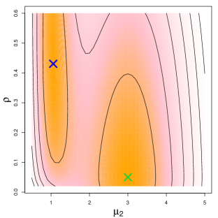
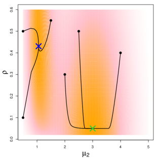
Figure 1: Log-likelihood function of fitting a 2-Gaussian mixture model to a data that is generated from a 3-Gaussian mixture model. The true distribution has a density function: $p_{0}(x)=0.5\phi(x;0,0.2^{2})+0.45\phi(x;0.75,0.2^{2})+0.05\phi(x;3,0.2^{2})$, where $\phi(x;\mu,\sigma^{2})$ is the density of a Gaussian with center $\mu$ and variance $\sigma^{2}$. We fit a 2-Guassian mixture with the center of the first Gaussian being set to $0$ and the variance of both Gaussians being $0.2^{2}$. The parameters of interest are the center of the second Gaussian $\mu_{2}$ and the proportion of the second Gaussian $\rho$. Namely, the log-likelihood function is $L(\mu_{2},\rho)={\mathbb{E}}(\log\left((1-\rho)\phi(X;0,0.2^{2})+\rho\phi(X;\mu_{2},0.2^{2})\right)),$ where $X$ has a PDF $p_{0}$. Left: Contour plot of the log-likelihood function $L(\mu_{2},\rho)$. Regions with orange color are where the log-likelihood function has a high value. The two local maxima are denoted by the blue and green crosses. Right: The trajectories of the gradient ascent method with multiple initial points. Each solid black dot is an initial point and the curve attached to it indicates the trajectory of the gradient ascent method starting from that initial point.

The goal of this paper is to analyze the statistical properties of this estimator. Note that we do not provide a solution to resolve the problem causing by multiple local maxima; instead, we attempt to analyze how the local maxima affect the performance of the estimator and the validity of a related statistical procedure. Although this estimator is not the MLE, it is commonly used in practice. To understand what population quantity this estimator is estimating, we study the behavior of estimators obtained from applying a gradient ascent algorithm to a likelihood function that has multiple local maxima. We investigate the underlying population quantity being estimated and analyze the properties of resulting CIs. Specifically, our main contributions are summarized as follows.

Main Contributions.

1. We derive the population quantity being estimated by the MLE when the likelihood function has multiple local maxima (Theorem 4 and 5).

2. We analyze the population quantity that a normal CI covers and study its coverage (Theorem 6).

3. We discuss how to use the bootstrap method to construct a meaningful CI and derive its coverage (Theorem 7).

4. We show that the CIs from inverting the likelihood ratio test, score test, and Wald test can be different (Section 3.3 and Figure 4).

5. We also discuss how to perform a two-sample test maintaining type-I error when the MLE is intractable (Section 3.4).

6. We analyze the probability that the EM algorithm recovers the actual MLE (Section 4) and study the coverage of its normal CI (Theorem 9).

7. We apply our developed framework to investigate the old faithful dataset (Section 5).

Related Work. The analysis of MLE under a multi-modal likelihood function has been analyzed for decades; see, for example, Redner (1981); Redner and Walker (1984); Sundberg (1974); Titterington et al. (1985). In the multi-modal case, finding the MLE is often accomplished by applying a gradient ascent method such as the EM-algorithm (Dempster et al., 1977; Wu, 1983; Titterington et al., 1985) with random initializations. The analysis of initializations and convergence of the gradient ascent method can be found in Lee et al. (2016); Panageas and Piliouras (2017); Jin et al. (2016); Balakrishnan et al. (2017). In our analysis, we use the Morse theory (Milnor, 1963; Morse, 1930; Banyaga and Hurtubise, 2013) to analyze the behavior of a gradient ascent algorithm. The analysis using the Morse theory is related to the work of Chazal et al. (2017); Mei et al. (2018); Chen et al. (2017).

Outline. We begin with providing the necessary background in Section 2. Then, we discuss how to perform statistical inference with local optima in Section 3. We extend our analysis to EM algorithm in Section 4. We provide data analysis in Section 5. Finally, we discuss issues and opportunities for further work in Section 6. In the appendix, we include a simulation study to investigate the effect of initialization (Section A) and a generalization to mode hunting problem (Section E) and all technical assumptions and proofs (Section G).

2 Background

In the first few sections, we will focus on an estimator that attempts to maximize the likelihood function. Let $X_{1},\cdots,X_{n}\sim P_{0}$ be a random sample. For simplicity, we assume that each $X_{i}$ is continuous. In parametric estimation, we impose a model on the underlying population distribution function $P(\cdot;\theta)$. This gives a parametrized probability density function $p(\cdot;\theta)$. The MLE estimates the parameter using

$$\widehat{\theta}_{MLE}=\underset{\theta}{\sf argmax}\,\,\widehat{L}_{n}(\theta)=\underset{\theta}{\sf argmax}\,\,\frac{1}{n}\sum_{i=1}^{n}\log p(X_{i};\theta),$$

which can be viewed as an estimator of the population MLE:

$$\theta_{MLE}=\underset{\theta}{\sf argmax}\,\,L(\theta)=\underset{\theta}{\sf argmax}\,\,{\mathbb{E}}(\log p(X_{1};\theta)).$$

When the likelihood function has multiple local modes (maxima), the MLE does not in general have a closed form; therefore, we need a numerical method to find it. A common approach is to apply a gradient ascent algorithm to the likelihood function with a randomly chosen initial point. To simplify our analysis, we study a continuous-time gradient ascent flow of the likelihood function (this is like conducting a gradient ascent with an infinitely small step size). When the likelihood function has multiple local maxima, the algorithm may converge to a local maximum rather than to the global maximum. As a result, we need to repeat the above procedure several times with different initial values and choose the convergent point with the highest likelihood value.

To study the behavior of a gradient ascent flow, we define the following quantities. Given an initial point $\theta^{\dagger}$, let $\widehat{\gamma}_{\theta^{\dagger}}:{\mathbb{R}}\rightarrow\Theta$ be a gradient flow such that

$$\widehat{\gamma}_{\theta^{\dagger}}(0)=\theta^{\dagger},\quad\widehat{\gamma}_{\theta^{\dagger}}^{\prime}(t)=\nabla\widehat{L}_{n}(\gamma_{\theta^{\dagger}}(t)).$$

Namely, the flow $\widehat{\gamma}_{\theta^{\dagger}}$ starts at $\theta^{\dagger}$ and moves according to the gradient direction of $\widehat{L}_{n}$. The stationary point $\widehat{\gamma}_{\theta^{\dagger}}(\infty)=\lim_{t\rightarrow\infty}\widehat{\gamma}_{\theta^{\dagger}}(t)$ is the destination of the gradient flow starting at $\theta^{\dagger}$. Different starting points lead to flows that may end at different points.

Because our initial points are chosen randomly, we view these initial points $\theta^{\dagger}_{1},\cdots,\theta^{\dagger}_{M}$ as IID draws from a distribution $\widehat{\Pi}_{n}(\cdot)$ (see, e.g., Chapter 2.12.2 of McLachlan and Peel 2004) that may depend on the original data $X_{1},\cdots,X_{n}$. The number $M$ denotes the number of the initializations. Later we will assume that $\widehat{\Pi}_{n}$ converges to a fixed distribution $\Pi$ when the sample size increases to infinity. Note that different initialization methods lead to a different distribution of $\widehat{\Pi}_{n}$. As an example, in the Gaussian mixture model, we often draw random points from the observed data as the initial centers of each mixture component. In this case, $\widehat{\Pi}_{n}$ can be viewed as the empirical distribution function.

By applying the gradient ascent to each of the $M$ initial parameters, we obtain a collection of stationary points $\widehat{\gamma}_{\theta^{\dagger}_{1}}(\infty),\cdots,\widehat{\gamma}_{\theta^{\dagger}_{M}}(\infty).$ The estimator is the one that maximizes the likelihood function so it can be written as

$$\widehat{\theta}_{n,M}={\sf argmax}_{\widehat{\gamma}_{\theta^{\dagger}_{\ell}}(\infty)}\left\{\widehat{L}_{n}\left(\widehat{\gamma}_{\theta^{\dagger}_{\ell}}(\infty)\right):\ell=1,\cdots,M\right\}.$$ (1)

In practice, we often treat $\widehat{\theta}_{n,M}$ as $\widehat{\theta}_{MLE}$ and use it to make inferences about the underlying population. However, unless the likelihood function is concave, there is no guarantee that $\widehat{\theta}_{n,M}=\widehat{\theta}_{MLE}$. Thus, our inferences and conclusions, which were based on treating $\widehat{\theta}_{n,M}$ as the MLE, could be problematic.

Algorithm 1 Gradient ascent with random initialization

1. Choose $\theta^{\dagger}$ randomly from a distribution $\widehat{\Pi}_{n}$.

2. Starting with $\theta^{\dagger}$, apply a gradient ascent algorithm to $\widehat{L}_{n}$ until it converges. Let $\widehat{\gamma}_{\theta^{\dagger}}(\infty)$ be the stationary point.

3. Repeat the above two steps $M$ times, leading to

$$\widehat{\gamma}_{\theta^{\dagger}_{1}}(\infty),\cdots,\widehat{\gamma}_{\theta^{\dagger}_{M}}(\infty).$$

4. Compute the corresponding log-likelihood value of each of them:

$$\widehat{L}_{n}\left(\widehat{\gamma}_{\theta^{\dagger}_{1}}(\infty)\right),\cdots,\widehat{L}_{n}\left(\widehat{\gamma}_{\theta^{\dagger}_{M}}(\infty)\right).$$

5. Choose the final estimator as

$$\widehat{\theta}_{n,M}={\sf argmax}_{\widehat{\gamma}_{\theta^{\dagger}_{\ell}}(\infty)}\left\{\widehat{L}_{n}\left(\widehat{\gamma}_{\theta^{\dagger}_{\ell}}(\infty)\right):\ell=1,\cdots,M\right\}.$$

2.1 Population-level Analysis

To better understand the inferences we make when treating $\widehat{\theta}_{n,M}$ as $\widehat{\theta}_{MLE}$, we start with a population level analysis over $\widehat{\theta}_{n,M}$. The population version of the gradient flow $\widehat{\gamma}_{\theta^{\dagger}}$ starting at $\theta^{\dagger}$ is a gradient flow $\gamma_{\theta^{\dagger}}(t)$ such that

$$\gamma_{\theta^{\dagger}}(0)=\theta^{\dagger},\quad\gamma_{\theta^{\dagger}}^{\prime}(t)=\nabla L(\gamma_{\theta^{\dagger}}(t)).$$

The destination of this gradient flow, $\gamma_{\theta^{\dagger}}(\infty)=\lim_{t\rightarrow\infty}\gamma_{\theta^{\dagger}}(t)$, is one of the critical points of $L(\theta)$.

For a critical point $m$ of $L$, we define the basin of attraction of $m$ as the collection of initial points where the gradient flow converges to $m$:

$$\mathcal{A}(m)=\{\theta\in\Theta:\gamma_{\theta}(\infty)=m\}.$$

Namely, $\mathcal{A}(m)$ is the region where the (population) gradient ascent flow converges to critical point $m$.

Throughout this paper, we assume that $L$ is a Morse function and $L$ has a continuous second derivatives. That is, critical points of $L$ are non-degenerate (well-separated). By the stable manifold theorem (e.g., Theorem 4.15 of Banyaga and Hurtubise 2013), $\mathcal{A}(m)$ is a $k$-dimensional manifold, where $k$ is the number of negative eigenvalues of $H(m)$, the Hessian matrix of $L(\cdot)$ evaluated at $m$. Thus, the Lebesgue measure of $\mathcal{A}(m)$ is non-zero only when $m$ is a local maximum. Because of this fact, we restrict our attention to local maxima and ignore other types of critical points; a randomly chosen initial point has probability zero of falling within the basin of attraction of a critical point that is not a local maximum when $\widehat{\Pi}_{n}$ is continuous. Note that a similar argument also appears in Lee et al. (2016) and Panageas and Piliouras (2017). Let ${{\mathcal{C}}}$ be the collection of local maxima with

$${{\mathcal{C}}} =\{m_{1},\cdots,m_{K}\},$$

$$L(m_{1}) \geq L(m_{2})\geq\cdots L(m_{K}),$$

where $K$ is the number of local maxima. The population MLE is $m_{1}=\theta_{MLE}$.

Figure 2 provides an illustration of the critical points and the basin of attraction. The left panel displays the contour plot of a log-likelihood function. The three solid black dots are the local maxima ($m_{1},m_{2}$, and $m_{3}$), the three crosses are the critical points, and the empty box indicates a local minimum. In the middle panel, we display gradient flows from some starting points. The right panel shows the corresponding basins of attraction ($\mathcal{A}(m_{1})$, ${\mathcal{A}}(m_{2})$, and ${\mathcal{A}}(m_{3})$). Each color patch is a basin of attraction of a local maximum.

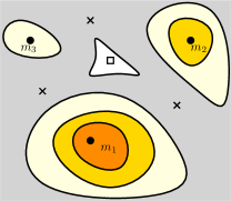
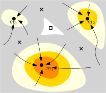
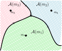
Figure 2: An illustration of critical points and basin of attractions. Left: the colored contours show the level sets of the log-likelihood function. The three sold black dots are the locations of local maxima ($m_{1},m_{2}$, and $m_{3}$); the crosses are the locations of saddle points; and the empty box indicates the location of a local minimum. Middle: gradient flows with different starting points. Each arrow indicates the gradient flow starting from an initial point that ends at a local maximum. Right: Basins of attractions of local maxima. Each color patch is the basin of attraction of a local maximum. Note that by the Morse theory, saddle points and local minima will be on the boundary of basins of attraction of local maxima.

For the $\ell$-th local maximum, we define the probability

$$q^{\pi}_{\ell}=\Pi(\mathcal{A}(m_{\ell}))=\int_{\mathcal{A}(m_{\ell})}d\Pi(\theta),$$ (2)

where $\Pi$ is the population version of $\widehat{\Pi}_{n}$ (i.e., $\widehat{\Pi}_{n}$ converges to $\Pi$ in the sense of assumption (A4) in the Appendix D.1). $q^{\pi}_{\ell}$ is the probability that the initialization method chooses an initial point within the basin of attraction of $m_{\ell}$. Namely, $q^{\pi}_{\ell}$ is the chance that the gradient ascent flow converges to $m_{\ell}$ from a random initial point. Note that we add a superscript $\pi$ to $q^{\pi}_{\ell}$ to emphasize the fact that this quantity depends on how we choose the initialization approach. Varying the initialization method leads to different probabilities $q^{\pi}_{\ell}$.

We define a ‘cumulative’ probability of the top $N$ local maxima as $Q^{\pi}_{N}=\sum_{\ell=1}^{N}q^{\pi}_{\ell},$ where $q^{\pi}_{\ell}$ is defined in equation (2). The quantity $Q^{\pi}_{N}$ plays a key role in our analysis because it is the probability of seeing one of the top $N$ local maxima after applying the gradient ascent method with a single initialization. Note that $q^{\pi}_{1}=Q^{\pi}_{1}$ is the probability of selecting an initial parameter value within the basin of attraction of the MLE, which is also the probability of obtaining the MLE with only one initialization. Later we will give a bound on the number of initializations we need in order to obtain the MLE with a high probability (Proposition 2).

Because the estimator $\widehat{\theta}_{n,M}$ is constructed by $M$ initializations, we introduce a population version of it. Let $\theta^{\dagger}_{1},\cdots,\theta^{\dagger}_{M}\sim\Pi$ be the initial points and let $\gamma_{\theta^{\dagger}_{1}}(\infty),\cdots,\gamma_{\theta^{\dagger}_{M}}(\infty)$ be the corresponding destinations. The quantity

$$\bar{\theta}_{M}={\sf argmax}_{\gamma_{\theta^{\dagger}_{\ell}}(\infty)}\left\{L\left(\gamma_{\theta^{\dagger}_{\ell}}(\infty)\right):\ell=1,\cdots,M\right\}.$$

is the population analog of $\widehat{\theta}_{n,M}$.

Due to the fact that $\bar{\theta}_{M}$ is constructed by $M$ initializations, it may not be the population MLE $\theta_{MLE}$. However, it is still the best among all these $M$ candidates so it should be one of the top local maxima in terms of the likelihood value. Let ${{\mathcal{C}}}_{N}=\{m_{1},\cdots,m_{N}\}$ be the top $N$ local maxima, where $N\leq K$ and $L(m_{1})\geq\cdots\geq L(m_{K})$. By simple algebra, we have

$$P(\bar{\theta}_{M}\in{{\mathcal{C}}}_{N})=1-P(\bar{\theta}_{M}\notin{{\mathcal{C}}}_{N})=1-(1-Q^{\pi}_{N})^{M}.$$

Given any fixed number $N$, such a probability converges to $1$ as $M\rightarrow\infty$ when $\Pi$ covers the basin of attraction of every local maximum. Therefore, we can pick $N=1$ and choose $M$ sufficiently large to ensure that we obtain the MLE with an overwhelming probability. However, when $M$ is finite, the chance of obtaining the population MLE could be slim.

To acknowledge the effect from the initializing $M$ times, we introduce a new quantity called the precision level, denoted as $\delta>0$. Given a precision level $\delta$, we define an integer

$$N^{\pi}_{M,\delta}=\min\{N:(1-Q^{\pi}_{N})^{M}\leq\delta\}$$

that can be interpreted as: with a probability of at least $1-\delta$, $\bar{\theta}_{M}$ is among the top $N^{\pi}_{M,\delta}$ local maxima. We further define

$${{\mathcal{C}}}^{\pi}_{M,\delta}={{\mathcal{C}}}_{N^{\pi}_{M,\delta}},$$ (3)

which satisfies

$$P(\bar{\theta}_{M}\in{{\mathcal{C}}}^{\pi}_{M,\delta})\geq 1-\delta.$$

Namely, with a probability of at least $1-\delta$, $\bar{\theta}_{M}$ recovers one element of ${{\mathcal{C}}}^{\pi}_{M,\delta}$. We often want $\delta$ to be small because later we will show that common CIs have an asymptotic coverage $1-\alpha-\delta$ containing an element of ${{\mathcal{C}}}^{\pi}_{M,\delta}$ (Section 3.1). If we want to control the type-I error to be, say $5\%$, we may want to choose $\alpha=2.5\%$ and $\delta=2.5\%$.

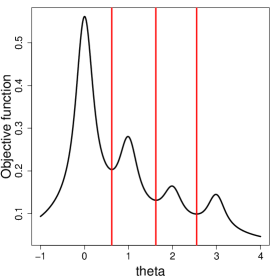
Figure 3: A modal regression method to the mixture regression problem. Left: we display a data generated by a 4-mixture regression model. Right: the objective function of the linear modal regression as a function of the parameter $\theta$. The three red vertical lines display the boundary of basins of attraction of the four local modes.

Example 1 (Modal regression).

To illustrate the idea, consider a regression problem where we observe $(X_{1},Y_{1}),\cdots,(X_{n},Y_{n})$ and the goal is to fit a linear model of the conditional mode of $Y$ given $X$. This problem is called linear modal regression (Yao and Li, 2014; Feng et al., 2020; Chen, 2018). Suppose that our data is generated by the following mixture model (intercept is 0):

$$Y=\theta X+\epsilon,\quad X\sim{\sf Uni}[0,1],\quad\epsilon\sim N(0,0.05^{2}).$$

However, $\theta$ is also random such that $P(\theta=0)=0.6,P(\theta=1)=0.2,P(\theta=2)=P(\theta=3)=0.1$. Namely, it is a mixture of 4 component regression problem and the left panel of Figure 3 shows a scatter plot of the data. It is known that (Chen, 2018) if we are looking for the conditional (global) mode of $Y$ given $X$, we can maximize the following objective function:

$$\ell_{n}(\theta)=\frac{1}{nh}\sum_{i=1}^{n}K\left(\frac{Y_{i}-\theta X_{i}}{h}\right).$$

The right panel plots $\ell_{n}(\theta)$ when we choose $h=0.1$ and $K$ to be the Gaussian kernel. The 4 local modes correspond to the 4 mixture components. The global mode is $\theta_{MLE}=m_{1}=0$, which corresponds to the component with the highest proportion. There are three other local modes $m_{2}=1,m_{3}=2,m_{4}=3$. The three vertical lines in the right panel indicate the boundaries of basins of attraction of different modes; they correspond to $\theta=0.62,1.62,2.55$. So the basin corresponding to the global mode is $\mathcal{A}(m_{1})=(-\infty,0.62)$.

Suppose that we randomly initialize the starting point within $[-1,4]$ (i.e., $\Pi\sim{\sf Uni}[-1,4]$), then $q^{\pi}_{1}=\Pi((-\infty,0.62))=1.62\times 0.2=0.324$ and $q^{\pi}_{2}=0.2,q^{\pi}_{3}=0.186,q^{\pi}_{4}=0.29$. Therefore, we only have around $32\%$ chance of getting the actual maximizer if we only initialize it once. Suppose that $\delta=1\%$ and we randomly initialize the program $4$ times, we obtain $N^{\pi}_{4,0.01}=3$ so ${{\mathcal{C}}}^{\pi}_{4,0.01}=\{m_{1},m_{2},m_{3}\}$. To ensure ${{\mathcal{C}}}^{\pi}_{M,0.01}=\{m_{1}\}$, we need at least $M=12$ random initializations (this corresponds to $(1-0.324)^{12}\approx 0.0091<\delta=0.01$).

The above example is a particularly simple case (one dimensional so we can clearly see the landscape of the objective function), so we can work out the minimal number $M$ to guarantee a probability of at least $1-\delta$ of finding the global mode (i.e., ${{\mathcal{C}}}^{\pi}_{M,\delta}=\{\theta_{MLE}\}$). In Section 3.5, we propose a practical rule of choosing $M$ based on our judgement of the problem. In what follows, we provide a theoretical upper bound of the minimal number using the curvature around the global mode. Let $\nabla_{\nu}$ denotes the directional derivative with respect to $\nu\in\mathbb{S}_{d}$, where $\mathbb{S}_{d}=\{\nu\in{\mathbb{R}}^{d}:\|\nu\|=1\}$ is the collection of all unit vectors in $d$ dimensions. When either $M$ or $\delta$ increase, the set ${{\mathcal{C}}}^{\pi}_{M,\delta}$ may shrink. Under smoothness conditions of $L$, a sufficiently large $M$ ensures ${{\mathcal{C}}}^{\pi}_{M,\delta}=\{\theta_{MLE}\}$ as described in the following proposition.

Proposition 2.

Assume that $\Theta$ is a compact parameter space. Assume all eigenvalues of $H(\theta_{MLE})=\nabla\nabla L(\theta_{MLE})$ are less than $-\lambda_{0}$ for some positive constant $\lambda_{0}$ and

$$\sup_{\theta\in\Theta}\sup_{\nu_{1},\nu_{2},\nu_{3}\in\mathbb{S}_{d}}\left|\nabla_{\nu_{1}}\nabla_{\nu_{2}}\nabla_{\nu_{3}}L(\theta)\right|<c_{3}.$$

Moreover, assume that $\theta_{MLE}$ is unique within $\Theta$. Then for every $\delta>0$, $P\left({{\mathcal{C}}}^{\pi}_{M,\delta}=\{\theta_{MLE}\}\right)\geq 1-\delta$ when $M\geq\frac{\log\delta}{\log\left(1-\Pi\left(B(\theta_{MLE},\frac{\lambda_{0}}{c_{3}})\right)\right)},$ where $B(\theta,r)=\{x\in\Theta:\|x-\theta\|_{2}\leq r\}$ is the ball centered at $\theta$ with a radius $r$.

Proposition 2 describes a desirable scenario: when $M$ is sufficiently large, with a probability of at least $1-\delta$ the set ${{\mathcal{C}}}^{\pi}_{M,\delta}$ contains only the MLE.

If the uniqueness assumption is violated, i.e., there are multiple parameters attaining the maximum value of the likelihood function, then the set ${{\mathcal{C}}}^{\pi}_{M,\delta}$ converges to the collection of all these maxima in probability when $M\rightarrow\infty$. One common scenario in which we encounter this situation is in mixture models where permuting some parameters results in the same model (this is known as the label switching problem in Titterington et al. 1985).

2.2 Sample-level Analysis

In this section, we show that $\widehat{\theta}_{n,M}$ converges to an element of $\mathcal{C}^{\pi}_{M,\delta}$ with a probability at least $1-\delta$. We first introduce some generic assumptions. We define the projection distance $d(x,A)=\inf_{y\in A}\|x-y\|$ for any point $x$ and any set $A$. For a set $A$ and a scalar $r$, define $A\oplus r=\{x:d(x,A)\leq r\}$.

We start with a useful lemma which states that with a high probability (a probability tending to $1$ as the sample size increases), the local maxima of $\widehat{L}_{n}$ and the local maxima of $L$ have a one-to-one correspondence. Denote the collection of local maxima of $\widehat{L}_{n}$ as $\widehat{{{\mathcal{C}}}}=\{\widehat{m}_{1},\cdots,\widehat{m}_{\widehat{K}}\}$ such that $\widehat{L}_{n}(\widehat{m}_{1})\geq\cdots\geq\widehat{L}_{n}(\widehat{m}_{\widehat{K}}),$ where $\widehat{K}$ is the number of local maxima of $\widehat{L}_{n}$. Note that by definition, $\widehat{m}_{1}=\widehat{\theta}_{MLE}$. Let

$$\epsilon_{1,n} =\sup_{\theta\in\Theta}\left\|\nabla\widehat{L}_{n}(\theta)-\nabla L(\theta)\right\|_{\max},$$

$$\epsilon_{2,n} =\sup_{\theta\in\Theta}\left\|\nabla\nabla\widehat{L}_{n}(\theta)-\nabla\nabla L(\theta)\right\|_{\max},$$

be the bounds on gradient and Hessian.

Lemma 3.

Assume (A1) and (A3) in Appendix D.1. Then there exists a constant $C_{0}$ such that when $\epsilon_{1,n},\epsilon_{2,n}<C_{0}$, $\widehat{K}=K$ and for every $\ell=1,\cdots,K$,

$$\|\widehat{m}_{\ell}-m_{\ell}\|<\min\left\{\min_{j\neq\ell}\|\widehat{m}_{\ell}-m_{j}\|,\min_{j\neq\ell}\|\widehat{m}_{j}-m_{\ell}\|\right\}.$$

This result appears in many places in the literature so we will omit the proof in this exposition. Interested readers are encourage to consult Chazal et al. (2017); Mei et al. (2018); Chen et al. (2017). Note that in most cases, we in fact have a stronger result than what Lemma 3 suggests – not only is there a one-to-one correspondence between a pair of estimated and population local maxima, but also between pairs of other types of critical points.

The following theorem provides a bound on the distance from $\widehat{\theta}_{n,M}$ to ${{\mathcal{C}}}^{\pi}_{M,\delta}$.

Theorem 4.

Assume (A1-4) in Appendix D.1 and let $\epsilon_{3,n},\epsilon_{4,n}$ be the two bounds in Assumption (A4) in Appendix D.1. Let $C_{0}$ be the constant in Lemma 3 and

$$\xi_{n}=P(\epsilon_{1,n}\geq C_{0}\mbox{ or }\epsilon_{2,n}\geq C_{0}).$$

When $\epsilon_{1,n},\cdots,\epsilon_{4,n}$ are non-random, with a probability of at least $1-\delta-\xi_{n}+O(\epsilon_{1,n}+\epsilon_{3,n}+\epsilon_{4,n})$,

$$d\left(\widehat{\theta}_{n,M},{{\mathcal{C}}}^{\pi}_{M,\delta}\right)=O\left(\epsilon_{1,n}\right).$$

Moreover, when $\epsilon_{1,n},\cdots,\epsilon_{4,n}$ are random and there exists $\eta_{n,j}(t)$ such that

$$P(\epsilon_{j,n}>t)\leq\eta_{n,j}(t)\quad\mbox{for }j=1,\cdots,4,$$

then for any sequence $t_{n}\rightarrow 0$, with a probability of at least $1-\delta-\xi_{n}+O(t_{n})-\sum_{j=1,3,4}\eta_{n,j}(t_{n})$,

$$d\left(\widehat{\theta}_{n,M},{{\mathcal{C}}}^{\pi}_{M,\delta}\right)=O_{P}\left(\epsilon_{1,n}\right).$$

In the first claim ($\epsilon_{1,n},\cdots,\epsilon_{4,n}$ are non-random), the probability comes from the randomness of initializations. In the second claim ($\epsilon_{1,n},\cdots,\epsilon_{4,n}$ are random), the probability statement accounts for both the randomness of initializations and $\epsilon_{1,n},\cdots,\epsilon_{4,n}$.

In many applications, the probability $\xi_{n}$ is very small because that statement is true when both $\epsilon_{1,n},\epsilon_{2,n}$ are less than a fixed threshold (see Lemma 16 of Chazal et al. 2017). Further, the chance that these two quantities are less than a fixed number has a probability of $1-e^{-C\cdot a_{n}}$ for some $a_{n}\rightarrow\infty$ as $n\rightarrow\infty$ and $C>0$ so often $\xi_{n}$ can be ignored.

When we made further assumptions of the likelihood function to obtain a $\sqrt{n}$ rate (assumptions (A3L) and (A4L) in Appendix D.1), we have the following result on a concrete rate.

Theorem 5.

Assume (A1), (A2) (A3L), and (A4L) in Appendix D.1. Then when $n\rightarrow\infty$, with a probability of at least $1-\delta-O\left(\sqrt{\frac{\log n}{n}}\right)$,

$$d\left(\widehat{\theta}_{n,M},{{\mathcal{C}}}^{\pi}_{M,\delta}\right)=O_{P}\left(\frac{1}{\sqrt{n}}\right).$$

Theorem 5 bounds the distance from the estimator to an element of ${{\mathcal{C}}}^{\pi}_{M,\delta}$ when $M$ initializations are used. Note that if $M$ is sufficiently large (so Proposition 2 holds), then we can claim that $\|\widehat{\theta}_{n,M}-\theta_{MLE}\|=O_{P}\left(\frac{1}{\sqrt{n}}\right)$ with a probability around $1-\delta$.

3 Statistical Inference

In this section we study the procedure of making inferences when the likelihood function has multiple maxima.

To simplify the problem of constructing CIs, we focus on constructing CIs of $\tau_{MLE}=\tau(\theta_{MLE})$, where $\tau:\Theta\rightarrow{\mathbb{R}}$ is a known function. We estimate $\tau_{MLE}$ using $\widehat{\tau}_{MLE}=\tau(\widehat{\theta}_{n,M})$. Recall that ${{\mathcal{C}}}^{\pi}_{M,\delta}$ from equation (3) is the top local modes that we can discover with a precision level $1-\delta$ and $M$ initializations and $\Pi$ initialization method. Moreover, we define

$$\tau\left({{\mathcal{C}}}^{\pi}_{M,\delta}\right)=\{\tau(\theta):\theta\in{{\mathcal{C}}}^{\pi}_{M,\delta}\}.$$

The set $\tau\left({{\mathcal{C}}}^{\pi}_{M,\delta}\right)$ will be the population quantity that the CIs are covering.

3.1 Normal Confidence Interval

A naive approach to constructing a CI is to estimate the variance of $\tau(\widehat{\theta}_{n,M})$ and invert it into a CI. Such CIs are in one-dimensional space and are based on the asymptotic normality of the MLE (Redner and Walker, 1984):

$$\sqrt{n}\left(\widehat{\theta}_{MLE}-\theta_{MLE}\right)\overset{D}{\rightarrow}N(0,\sigma^{2}),$$

for some $\sigma^{2}>0$. In practice, we only have access to $\widehat{\theta}_{n,M}$, not $\widehat{\theta}_{MLE}$, so we replace $\widehat{\theta}_{MLE}$ by $\widehat{\theta}_{n,M}$ and construct a CI using the normality. This is perhaps the most common approach to the construction of a CI and the representation of the error of estimation (see Chapter 2.15 and 2.16 in McLachlan and Peel 2004 for examples of mixture models). However, we will show that when the likelihood function has multiple local maxima, this CI undercovers for $\tau_{MLE}$ and has $1-\alpha-\delta$ coverage for an element in $\tau({{\mathcal{C}}}_{M,\delta}^{\pi})$.

To fully describe the construction of this normal CI, we begin with an analysis of the asymptotic covariance of the MLE. Let $S(\theta)=\nabla L(\theta)$ be the score function and $H(\theta)=\nabla S(\theta)$ be the Hessian matrix of the log-likelihood function. Moreover, let $S(\theta|X_{i})=\nabla\log p(X_{i};\theta)$ and $H(\theta|X_{i})=\nabla S(\theta|X_{i})$. The MLE $\widehat{\theta}_{MLE}$ has an asymptotic covariance matrix

$${\sf Cov}(\widehat{\theta}_{MLE})=H(\theta_{MLE})^{-1}{\mathbb{E}}(S(\theta_{MLE}|X_{1})S(\theta_{MLE}|X_{1})^{T})H(\theta_{MLE})^{-1}+o(1).$$

Note that under regularity conditions,

$$H(\theta_{MLE})=-{\mathbb{E}}(S(\theta_{MLE}|X_{1})S(\theta_{MLE}|X_{1})^{T})=-I(\theta_{MLE})$$

is the Fisher’s information matrix, which further implies ${\sf Cov}(\widehat{\theta}_{MLE})=I^{-1}(\theta_{MLE}).$ However, when the model is mis-specified, $H(\theta_{MLE})\neq I(\theta_{MLE})={\mathbb{E}}(S(\theta_{MLE}|X_{1})S(\theta_{MLE}|X_{1})^{T})$, and in this case, we cannot use the information matrix to construct a normal CI.

Using the delta method (Van der Vaart, 1998; Wasserman, 2006), the variance of $\tau(\widehat{\theta}_{MLE})$ is

$${\sf Var}\left(\tau(\widehat{\theta}_{MLE})\right)=g_{\tau}^{T}(\theta_{MLE}){\sf Cov}(\widehat{\theta}_{MLE})g_{\tau}(\theta_{MLE}),$$

where $g_{\tau}(\theta)=\nabla\tau(\theta)$.

Thus, given an estimator $\widehat{\theta}_{n,M}$, we can estimate the covariance matrix using

$$\widehat{{\sf Cov}}(\widehat{\theta}_{n,M}) =\widehat{H}_{n}(\widehat{\theta}_{n,M})^{-1}\left(\frac{1}{n}\sum_{i=1}^{n}S(\widehat{\theta}_{n,M}|X_{i})S(\widehat{\theta}_{n,M}|X_{i})^{T}\right)\widehat{H}_{n}(\widehat{\theta}_{n,M})^{-1},$$ (4)

$$\widehat{H}_{n}(\theta) =\frac{1}{n}\sum_{i=1}^{n}H(\theta|X_{i}).$$

And the CI is

$$C_{n,\alpha}=\left\{t:\sqrt{n}\left|\frac{t-\tau(\widehat{\theta}_{n,M})}{g_{\tau}^{T}(\widehat{\theta}_{n,M})\widehat{\sf Cov}(\widehat{\theta}_{n,M})g_{\tau}(\widehat{\theta}_{n,M})}\right|\leq z_{1-\alpha/2}\right\},$$ (5)

where $z_{\alpha}$ is the $\alpha$ quantile of a standard normal distribution. Note that under suitable assumptions, one can also use Fisher’s information matrix or the empirical information matrix to replace $\widehat{{\sf Cov}}(\widehat{\theta}_{n,M})$.

However, because $\widehat{\theta}_{n,M}$ is never guaranteed to be the MLE, $C_{n,\alpha}$ may not contain the population MLE with the right coverage. In what follows, we show that $C_{n,\alpha}$ has an asymptotic $1-\alpha-\delta$ coverage of covering an element of $\tau\left({{\mathcal{C}}}^{\pi}_{M,\delta}\right)$ and $1-\alpha-(1-q^{\pi}_{1})^{M}$ coverage for covering the MLE, where $q^{\pi}_{1}=\Pi({\mathcal{A}}(\theta_{MLE}))$ is defined in equation (2).

Theorem 6.

Assume (A1), (A2), (A3L), (A4L), (A5), and (T) in Appendix D.1 and D.2. Then $P(C_{n,\alpha}\cap\tau\left({{\mathcal{C}}}^{\pi}_{M,\delta}\right)\neq\emptyset)\geq 1-\alpha-\delta-O\left(\sqrt{\frac{\log n}{n}}\right).$ Thus, by choosing $\delta=(1-q^{\pi}_{1})^{M}$, we have

$$P(\tau_{MLE}\in C_{n,\alpha})\geq 1-\alpha-(1-q^{\pi}_{1})^{M}-O\left(\sqrt{\frac{\log n}{n}}\right).$$

The population quantity covered by the normal CI is given by the fact that $C_{n,\alpha}$ has an asymptotic $1-\alpha-\delta$ coverage for an element of $\tau\left({{\mathcal{C}}}^{\pi}_{M,\delta}\right)$. The quantities $\alpha$ and $\delta$ play similar roles in terms of coverage but they have different meanings. The quantity $\alpha$ is the conventional confidence level, which aims to control the fluctuation of the estimator. On the other hand, $\delta$ is the precision level that corrects for the multiple local optima.

When $M$ is sufficiently large (greater than the bound given in Proposition 2), Proposition 2 guarantees that we asymptotically have at least $1-\alpha-\delta$ coverage of the population MLE. Equivalently, when $\delta$ is sufficiently small ($\delta\leq(1-q^{\pi}_{1})^{M}\Rightarrow{{\mathcal{C}}}^{\pi}_{M,\delta}=\{\theta_{MLE}\}$), the first assertion implies the second assertion: $C_{n,\alpha}$ has a coverage of $1-\alpha-(1-q^{\pi}_{1})^{M}$ of containing $\tau_{MLE}$.

3.2 Bootstrap

The bootstrap method (Efron, 1982, 1979) is a common approach for constructing a CI. While there are many variants of bootstrap, we focus on the empirical bootstrap with the percentile approach.

When applying a bootstrap approach to an estimator that requires multiple initializations (such as our estimator or the estimator from an EM-algorithm), there is always a question: How should we choose the initial point for each bootstrap sample? Should we rerun the initialization several times to pick the highest value for each bootstrap sample?

Based on the following arguments, we recommend using the estimator of the original sample, $\widehat{\theta}_{n,M}$, as the initial point for every bootstrap sample. The purpose of using the bootstrap is to approximate the distribution of the estimator $\widehat{\theta}_{n,M}$. In the M-estimator theory (Van der Vaart, 1998), we know that the variation of $\widehat{\theta}_{n,M}$ is caused by the randomness of the function $\widehat{L}_{n}(\theta)$ around $\widehat{\theta}_{n,M}$. Thus, to make sure the bootstrap approximates such randomness, we need to ensure that the bootstrap estimator $\widehat{\theta}^{*}_{n,M}$ is around $\widehat{\theta}_{n,M}$ so the distribution of $\widehat{\theta}^{*}_{n,M}-\widehat{\theta}_{n,M}$ approximates the distribution of $\widehat{\theta}_{n,M}-\theta^{\dagger}$ for some $\theta^{\dagger}\in{{\mathcal{C}}}$. By Lemma 3, we know that there is a local maximum $\widehat{\theta}^{*}$ of the bootstrap log-likelihood function that is close to $\widehat{\theta}_{n,M}$. Therefore, we need that the initial point to which we apply the gradient ascent method in the bootstrap sample is within the basin of attraction of $\widehat{\theta}^{*}$ asymptotically (with a probability tending to $1$ when the sample size $n\rightarrow\infty$). Because $\widehat{\theta}_{n,M}$ is close to $\widehat{\theta}^{*}$, $\widehat{\theta}_{n,M}$ will be within the basin of attraction of $\widehat{\theta}^{*}$ asymptotically; as a result, $\widehat{\theta}_{n,M}$ is a good initial point for the bootstrap sample.

Moreover, using the same initial point in every bootstrap sample avoids the problem of label switching (Redner and Walker, 1984). Label switching occurs when the distribution function is the same after permuting some parameters. For instance, in a Gaussian mixture model with equal variance and proportion, permuting the location parameters leads to the same model. When we use the same initial point in every bootstrap sample, we alleviate this problem.

Algorithm 2 Percentile bootstrap method

1. Let $\widehat{\theta}_{n,M}$ be the output from Algorithm 1.

2. Generate a bootstrap sample and let $\widehat{L}^{*}_{n}$ denote the bootstrap log-likelihood function.

3. Use $\widehat{\theta}_{n,M}$ as the initial point, apply the gradient ascent algorithm to $\widehat{L}^{*}_{n}$ until it converges. Let $\widehat{\theta}^{*}_{n,M}$ be the convergent.

4. Repeat Step 2 and 3 $B$ times, leading to $\widehat{\theta}^{*(1)}_{n,M},\cdots,\widehat{\theta}^{*(B)}_{n,M}.$ Let $\tau(\widehat{\theta}^{*(1)}_{n,M}),\cdots,\tau(\widehat{\theta}^{*(B)}_{n,M})$ be the corresponding value of the parameter of interest.

5. Compute the quantile

$$\widehat{\omega}_{1-\alpha}=\widehat{G}_{\omega}^{-1}(1-\alpha),\quad\widehat{G}_{\omega}(s)=\frac{1}{B}\sum_{\ell=1}^{B}I(\tau(\widehat{\theta}^{*(\ell)}_{n,M,})\leq s).$$

6. Form the CI as $\widehat{C}_{n,\alpha}^{*}=\left[\widehat{\omega}_{\alpha/2},\widehat{\omega}_{1-\alpha/2}\right].$

Now we describe the formal bootstrap procedure. Let $X_{1}^{*},\cdots,X^{*}_{n}$ be a bootstrap sample. We first calculate the bootstrap log-likelihood function $\widehat{L}_{n}^{*}$. Next, we start a gradient ascent flow from the initial point $\widehat{\theta}_{n,M}$. The gradient ascent flow leads to a new local maximum, denoted as $\widehat{\theta}^{*}_{n,M}$. By evaluating the function $\tau(\cdot)$ at this new local maximum, we obtain a bootstrap estimate of the parameter of interest, $\tau(\widehat{\theta}^{*}_{n,M})$. We repeat the above procedure many times and construct a CI using the upper and lower $\alpha/2$ quantile of the distribution of $\tau(\widehat{\theta}^{*}_{n,M})$. Namely, let

$$\widehat{\omega}_{1-\alpha}=\widehat{G}^{-1}(1-\alpha),\quad\widehat{G}_{\omega}(s)=P(\tau(\widehat{\theta}^{*}_{n,M})\leq s|X_{1},\cdots,X_{n}).$$

The CI is $\widehat{C}_{n,\alpha}^{*}=\left[\widehat{\omega}_{\alpha/2},\widehat{\omega}_{1-\alpha/2}\right].$ Algorithm 2 outlines the procedure of this bootstrap approach.

A benefit of this CI is that $\widehat{C}_{n,\alpha}^{*}$ does not require any knowledge about the variance of $\widehat{\theta}_{n,\alpha}$. When the variance is complicated or does not have a closed form, being able to construct a CI without knowledge of the variance makes this approach particularly appealing.

Theorem 7.

Assume (A1), (A2), (A3L), (A4L), (A5), and (T) in Appendix D.1 and D.2. Let $\widehat{C}_{n,\alpha}^{*}$ be defined as the above. Then

$$P(\widehat{C}^{*}_{n,\alpha}\cap\tau({{\mathcal{C}}}_{M,\delta}^{\pi})\neq\emptyset)\geq 1-\alpha-\delta-O\left(\sqrt{\frac{\log n}{n}}\right).$$

Therefore, by choosing $\delta=(1-q^{\pi}_{1})^{M}$, where $q^{\pi}_{1}$ is defined in Theorem 6, we conclude that

$$P(\tau_{MLE}\in\widehat{C}^{*}_{n,\alpha})\geq 1-\alpha-(1-q^{\pi}_{1})^{M}-O\left(\sqrt{\frac{\log n}{n}}\right).$$

The conclusions of Theorem 7 are similar to those of Theorem 6: under appropriate conditions, with a (asymptotic) coverage $1-\alpha-\delta$, the CI covers an element of $\tau({{\mathcal{C}}}_{M,\delta}^{\pi})$, and with a coverage $1-\alpha-(1-q^{\pi}_{1})^{M}$, the CI covers $\tau_{MLE}$.

Remark 1.

There are many other variants of bootstrap approaches and Algorithm 2 describes only a simple one. A common alternative to the method so far presented is bootstrapping the pivotal quantity (also known as the studentized pivotal approach in Wasserman 2006 and the percentile-$t$ approach in Hall 2013). In certain scenarios, bootstrapping a pivotal quantity leads to a CI with a higher order accuracy (namely., the coverage will be $1-\alpha-O\left(\frac{1}{n}\right)$). However, we may not have such a property because the bottleneck of the coverage error $O\left(\sqrt{\frac{\log n}{n}}\right)$ comes from the uncertainty of the basins of attraction. Such uncertainty may not be reduced when using the pivotal approach.

3.3 Confidence Intervals by Inverting a Test

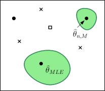
(a) Likelihood ratio test.

(b) Score test.

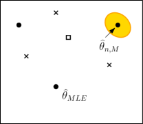
(c) Wald test.

Figure 4: Illustration of CIs from inverting a test. The black dots are local maxima of the estimated likelihood function. The black crosses are saddle points. The empty box is a local minimum. Assume that the estimator we compute, $\widehat{\theta}_{n,M}$, is the local maximum in the top-right corner and the actual MLE is the local maximum at the bottom. Left: The CI (green areas) from the likelihood ratio test. This CI contains not only the regions around our estimator but also regions around the actual MLE. Middle: The CI (purple areas) from the score test. This CI contains regions around each critical point because the gradient around every critical point is close to $0$. Right: The CI (yellow area) from the Wald test. This CI will be an ellipsoid around the estimator $\widehat{\theta}_{n,M}$. Note that this figure is only for the purpose of illustration; it was not created from a real dataset.

In this section, we introduce three CIs of $\tau_{MLE}$ created by inverting hypothesis tests. We consider three famous tests: the likelihood ratio test, the score test, and the Wald test. Although the three tests are asymptotically equivalent in a regular setting (when the likelihood function is concave and smooth), they lead to very different CIs when the likelihood function has multiple local maxima. Figure 4 provides an example illustrating these three CIs of a multi-modal likelihood function.

Because it is easier to invert a test for a CI of $\theta_{MLE}$, we focus on describing the procedure of constructing a CI of $\theta_{MLE}$ is this section. With a $1-\alpha$ CI of $\theta_{MLE}$, say $\widehat{\Theta}_{n,\alpha}$, one can easily invert it into a $1-\alpha$ CI of $\tau_{MLE}$ by

$$\widehat{\mathcal{T}}_{n,\alpha}=\left\{\tau(\theta):\theta\in\widehat{\Theta}_{n,\alpha}\right\}.$$ (6)

3.3.1 Likelihood ratio test

One classical approach to inverting a test to a CI is to use the likelihood ratio test (Owen, 1990). Such a CI is also called a likelihood region in Kim and Lindsay (2011).

Under appropriate conditions, the likelihood ratio test implies

$$2n(\widehat{L}_{n}(\widehat{\theta}_{MLE})-\widehat{L}_{n}(\theta_{MLE}))\overset{d}{\rightarrow}\chi^{2}_{d},$$

where $\chi^{2}_{k}$ is a $\chi^{2}$ distribution with $k$ degrees of freedom and $d$ is the dimension of the parameter. This motivates a $1-\alpha$ CI of $\theta_{MLE}$ of the form

$$\Theta_{n,\alpha}^{0}=\left\{\theta:2n(\widehat{L}_{n}(\widehat{\theta}_{MLE})-\widehat{L}_{n}(\theta))\leq\zeta_{d,1-\alpha}\right\},$$

where $\zeta_{d,1-\alpha}$ is the $1-\alpha$ quantile of $\chi^{2}_{d}$.

In practice, we do not know the actual MLE $\widehat{\theta}_{MLE}$ and have only the estimator $\widehat{\theta}_{n,M}$. Therefore, we replace $\widehat{\theta}_{MLE}$ by $\widehat{\theta}_{n,M}$, leading to a CI

$$\widehat{\Theta}_{n,\alpha}=\{\theta:2n(\widehat{L}_{n}(\widehat{\theta}_{n,M})-\widehat{L}_{n}(\theta))\leq\zeta_{d,1-\alpha}\}.$$ (7)

The CI $\widehat{\Theta}_{n,\alpha}$ has asymptotic $1-\alpha$ converage for $\theta_{MLE}$, regardless of whether or not $\widehat{\theta}_{n,M}$ equals to $\widehat{\theta}_{MLE}$ because $\widehat{L}_{n}(\widehat{\theta}_{n,M})\leq\widehat{L}_{n}(\widehat{\theta}_{MLE})$ implies $\widehat{\Theta}_{n,\alpha}\supset\Theta_{n,\alpha}^{0}$. Because the set $\Theta_{n,\alpha}^{0}$ is a CI with asymptotic $1-\alpha$ coverage of $\theta_{MLE}$, $\widehat{\Theta}_{n,\alpha}$ also enjoys this property. Thus, even when we only have a small number of initializations, the CI in equation (7) has the asymptotic (in terms of sample size) coverage.

The CI $\widehat{\Theta}_{n,\alpha}$ can be used to carry out a hypothesis test. Consider testing the null hypothesis

$$H_{0}:\tau_{MLE}=\tau_{0}\subset{\mathbb{R}}.$$ (8)

We can simply check if the set $\tau(\widehat{\Theta}_{n,\alpha})$ and $\tau_{0}$ intersects or not to decide if we can reject the null hypothesis. This controls the type-I error asymptotically.

Although $\widehat{\Theta}_{n,\alpha}$ is valid regardless of the number $M$, it is often very conservative and computationally intractable. When $\widehat{\theta}_{n,M}$ is not $\widehat{\theta}_{MLE}$, the set $\widehat{\Theta}_{n,\alpha}$ is often non-concave and composed of many disjoint regions, each of which corresponds to a local mode of $\widehat{L}_{n}$ with a likelihood value greater than $\widehat{\theta}_{n,M}$. See the left panel of Figure 4 for an illustration. Moreover, we do not know the exact locations of other regions because they correspond to the local modes whose basins of attraction contain no initial points when we apply the gradient ascent method.

Remark 2.

Although the number $M$ does not affect the coverage of $\widehat{\Theta}_{n,\alpha}$, it does affect the size of $\widehat{\Theta}_{n,\alpha}$. The higher log-likelihood value of the estimator $\widehat{\theta}_{n,M}$, the smaller $\widehat{\Theta}_{n,\alpha}$. This is because the CI includes all parameters whose likelihood values are greater than or equal to $\widehat{L}_{n}(\widehat{\theta}_{n,M})-\frac{1}{2n}\zeta_{d,1-\alpha}$. Thus, increasing $M$ does improve the CI, but not in the sense of coverage. This is a distinct feature compared to the bootstrap or normal CIs.

3.3.2 Score test

In addition to the likelihood ratio test, one may invert the score test (Rao, 1948) to obtain a CI. The score test is based on the following observation: when $\theta=\theta_{MLE}$ and the likelihood function is smooth,

$$n\cdot\nabla\widehat{L}_{n}(\theta)^{T}\widehat{I}_{n}(\theta)^{-1}\nabla\widehat{L}_{n}(\theta)\overset{d}{\rightarrow}\chi^{2}_{d},$$ (9)

where $\widehat{I}(\theta)=\frac{1}{n}\sum_{i=1}^{n}S(\theta|X_{i})S(\theta|X_{i})^{T}$ is the observed Fisher’s information matrix. Thus, we can construct a CI of $\theta_{MLE}$ via

$$\left\{\theta:n\cdot\nabla\widehat{L}_{n}(\theta)^{T}\widehat{I}_{n}(\theta)^{-1}\nabla\widehat{L}_{n}(\theta)\leq\zeta_{d,1-\alpha}\right\}$$

and then use it to construct a CI of $\tau_{MLE}$ as equation (6).

Although this CI is an asymptotically valid $1-\alpha$ CI, it tends to be very large because $\theta_{MLE}$ is not the only case in which equation (9) holds – all critical points, including local minima and saddle points, of $L(\cdot)$ satisfy this equation. Thus, this CI is the collection of regions around critical points, and as such it tends to be a complicated set of large total size. The middle panel of Figure 4 illustrates a CI from the score test. In terms of testing equation (8), we can use this CI or use the score test because the CI has the right coverage asymptotically.

3.3.3 Wald test

Another common approach to finding CIs is inverting the Wald test (Wald, 1943). It relies on the following fact:

$$n\cdot(\widehat{\theta}_{MLE}-\theta_{MLE})^{T}\widehat{\sf Cov}(\widehat{\theta}_{MLE})^{-1}(\widehat{\theta}_{MLE}-\theta_{MLE})\overset{d}{\rightarrow}\chi^{2}_{d}.$$

By the above property, a CI of $\theta_{MLE}$ is

$$\left\{\theta:n\cdot(\widehat{\theta}_{MLE}-\theta)^{T}\widehat{\sf Cov}(\widehat{\theta}_{MLE})^{-1}(\widehat{\theta}_{MLE}-\theta)\leq\zeta_{d,1-\alpha}\right\},$$

where $\widehat{\sf Cov}$ is defined in equation (4).

Because we do not have $\widehat{\theta}_{MLE}$ but only $\widehat{\theta}_{n,M}$, we use

$$\left\{\theta:n\cdot(\widehat{\theta}_{n,M}-\theta)^{T}\widehat{\sf Cov}_{n}(\widehat{\theta}_{n,M})^{-1}(\widehat{\theta}_{n,M}-\theta)\leq\zeta_{d,1-\alpha}\right\}$$

as the CI. By construction, this CI is an ellipsoid; see the right panel of Figure 4 for an illustration.

The CI that results from this inversion will be asymptotically the same as the normal CI so it has the same coverage property. Namely, the CI has asymptotic $1-\alpha-\delta$ coverage for covering one element of ${{\mathcal{C}}}^{\pi}_{M,\delta}$ and $1-\alpha-(1-q^{\pi}_{1})^{M}$ coverage for containing $\theta_{MLE}$.

Note that unlike the two previous CIs constructed from inverting tests that can be applied to testing the null hypothesis in equation (8), this CI may not control type-I error because it does not have the asymptotic coverage of covering $\theta_{MLE}$. The same issue also occurs in the normal CI $C_{n,\alpha}$ and the bootstrap CI $C^{*}_{n,\alpha}$.

Compared to the other two tests, the Wald test leads to a CI that can be represented easily – it is an ellipsoid around $\widehat{\theta}_{n,M}$. If we make further use of equation (6) to construct a CI of $\tau_{MLE},$ the result is an interval centered at the estimator $\tau(\widehat{\theta}_{n,M})$ so the CI can be succinctly expressed as the estimator plus and minus the standard error.

3.4 Two-Sample Test

We now explain how to do a two-sample test using a multi-modal likelihood function. In a two-sample test, we observe two sets of data $X_{1},\cdots,X_{n}\sim P_{X}$ and $Y_{1},\cdots,Y_{m}\sim P_{Y}$ and we would like to test if the two data sets are from the same distribution. That is, the null hypothesis being tested is

$$H_{0}:P_{X}=P_{Y}.$$ (10)

A common way of testing (10) is to fit a parametric model $P(\cdot;\theta)$ to both samples and then compare the fitted parameters. An advantage of this approach is that we can interpret the results based on the likelihood model. When rejecting $H_{0}$, we not only know that $H_{0}$ is not feasible, but also are able to describe the degree of difference between the two datasets by comparing their corresponding parameters.

Let $L_{X}(\theta)={\mathbb{E}}\log p(X_{1};\theta)$ and $L_{Y}(\theta)={\mathbb{E}}\log p(Y_{1};\theta)$ be the likelihood functions from the two populations. The null hypothesis in equation (10) implies

$$H_{0}:L_{X}=L_{Y}.$$ (11)

Because this equality is derived from equation (10), rejecting the null hypothesis in equation (11) implies that the null hypothesis in equation(10) should be also rejected.

A naive idea of how to test equation (11) is to compute the MLEs in both samples and then compare the MLEs to determine the significance. This method implicitly assumes that we can compute the actual MLEs. Indeed, the $H_{0}$ in equation (11) implies that the two MLEs should be the same so we can directly test the locations of MLEs. However, when $L_{X}$ or $L_{Y}$ is multi-modal, our estimators could be local maxima rather than the MLEs. Thus, the two estimators may be very different even if $H_{0}$ (in equation (11)) is true because the estimators happen to be different local maxima.

To ensure that the two estimators converge to the same destination when the null hypothesis $H_{0}$ is true, the two estimators must be estimating the same local maximum. A simple way is to choose the same initial point in both samples. We therefore recommend the procedure in Algorithm 3.

Algorithm 3 Two-sample test without the MLE

1. Pool both samples together, to form a joint sample $\{X_{1},\cdots,X_{n},Y_{1},\cdots,Y_{m}\}$.

2. Fit the log-likelihood model to this joint sample and apply the gradient ascent algorithm with a random initialization to find a local maximum.

3. Iterate the above procedure $M$ times and then select from among the local maxima that has the highest log-likelihood value. Denoted this local maximum by $\widehat{\theta}_{opt}$.

4. Now for each of the two samples, fit the likelihood function and apply the gradient ascent algorithm with initial point being $\widehat{\theta}_{opt}$. Let $\widehat{\theta}_{X}$ and $\widehat{\theta}_{Y}$ denote the destination of each of the two samples, respectively.

5. Compare $\widehat{\theta}_{X}$ and $\widehat{\theta}_{Y}$ using conventional two-sample test techniques.

In the first step, we combine the data from the two samples because under $H_{0}$, combining them gives us the largest sample from the population. The second and the third steps are the same as the algorithm described in Algorithm 1 to the pooled sample. The resulting estimator should be an estimator with a high likelihood value by Theorem 5. Under $H_{0}$, this estimator should also have a high value in terms of $L_{X}$ and $L_{Y}$. Moreover, because $\widehat{\theta}_{opt}$ is a local maximum of the pooled likelihood function and $H_{0}$ implies that $L_{X}$, $L_{Y}$, and pooled likelihood function are all the same, $\widehat{\theta}_{opt}$ should be close to both the local maximum of $L_{X}$ and the local maximum of $L_{Y}$ that correspond to the same local maximum of the underlying population likelihood function. Thus, both $\widehat{\theta}_{X}$ and $\widehat{\theta}_{Y}$ are close to the same local maximum of the underlying population likelihood function, so a comparison between them would control the type-I error (asymptotically).

We do not specify how to compare $\widehat{\theta}_{X}$ and $\widehat{\theta}_{Y}$ because there are many ways to perform this comparison. For instance, we can compare them by constructing their CIs and determining if the two CIs intersect. Or we can do a permutation test where the test statistics are some particular distance between them, e.g., $T_{1}=\|\widehat{\theta}_{X}-\widehat{\theta}_{Y}\|$.

3.5 A practical procedure of choosing $M$

As is shown in the above analysis, the choice of $M$ plays a key role in the coverage of a confidence set. Here we propose a practical procedure to choose $M$ based on the analyst’s judgement about $q_{1}^{\pi}$.

We first pick a the precision level $\delta$. A simple rule is to choose $\delta=1\%$ when the significance level $\alpha=5\%$ or $10\%$. Then we hypothesize a threshold $q^{*}$ such that we believe that $q_{1}^{\pi}\geq q^{*}$. Namely, we assume that the chance of initializing in the MLE’s basin of attraction is no smaller than $q^{*}$.

Under this threshold, to ensure the coverage deficiency is less than $\delta$, we need

$$(1-q^{*})^{M}\leq\delta\Rightarrow M\geq\frac{\log\delta}{\log(1-q^{*})}=M^{*}(\delta,q^{*}).$$

When $\delta$ and $q^{*}$ are given, the number of initializations needed is $M=M^{*}(\delta,q^{*})$.

Under $\delta=0.01(1\%)$, the above threshold becomes $M^{*}(0.01,q^{*})\approx\frac{4.6}{|\log(1-q^{*})|}.$ In the extreme case where $q^{*}\approx 0$ (i.e., the chance of obtaining the actual MLE is very small), we further have $|\log(1-q^{*})|\approx q^{*}$, so the above threshold becomes

$$M^{*}(0.01,q^{*})\approx 4.6/q^{*}.$$ (12)

The above threshold provides an easy-to-use reference rule of choosing $M$. For instance, suppose we believe that the chance of getting the MLE is no smaller than $0.1\%(10^{-3})$, then we need at least $M\geq 4.6\times 10^{3}=4,600$ initializations to ensure the coverage deficiency is less than $1\%$. The choice of $q^{*}$ should be determined by the analyst’s judgement about the problem.

In practice, when the dimension is large, $q^{*}$ is often small (see Section A and Table 1 in Appendix), so we need a large number of initializations to control this uncertainty. However, the threshold in equation (12) is independent of the dimension as long as $q^{*}$ is fixed. This implies that if we can design a method (such as using a strongly convex penalty) such that $q^{*}=q^{*}_{d}\rightarrow q^{*}_{0}$ when $d\rightarrow\infty$ and $q^{*}_{0}$ is not a tiny number, the bound $M^{*}(\delta,q^{*})$ can be small. For instance, if $q^{*}_{0}=0.1$ and $\delta=0.01$, we only need about $46$ initializations even if the dimension $d$ is large.

While the above analysis assumes $q^{*}$ to be fixed and non-random, this analysis can be applied to the case where $q^{*}=q^{*}_{n}$ is random and its distribution depends on $n$ as well. As long as we have a concentration bound such that $P(q^{*}_{n}>q^{*}_{\dagger,\delta})>1-\delta/2$ for some fixed quantity $q^{*}_{\dagger,\delta}$, we can plug $q^{*}_{\dagger,\delta}$ into (12) and use the revised bound $M^{*}(\delta/2,q^{*}_{\dagger,\delta})$ as the minimal number of initializations needed (we use $\delta/2$ to account for the randomness of $q^{*}_{n}$).

4 EM-Algorithm

In this section, we use the above framework to analyze estimators obtained from the EM-algorithm (Dempster et al., 1977; McLachlan and Peel, 2004; McLachlan and Krishnan, 2007). For simplicity, we consider a latent variable model, assuming that our observations are IID random variables $X_{1},\cdots,X_{n}$ from some unknown distribution and each individual has a latent variable $Z$. Namely, our dataset consists of pairs $(X_{1},Z_{1}),\cdots,(X_{n},Z_{n})$ that are IID from an unknown distribution function $P_{0}$ but the $Z_{1},\cdots,Z_{n}$ are unobserved.

With the latent variable, we assume that the density of $(X,Z)$ forms a parametric model $p_{\theta}(X,Z)$, where $\theta\in\Theta$ is the underlying parameter. We define

$$L(\theta|X,Z) =\log p_{\theta}(X,Z),$$

$$L(\theta|X) ={\mathbb{E}}(L(\theta|X,Z)|X),$$

$$L(\theta) ={\mathbb{E}}(L(\theta|X))={\mathbb{E}}(L(\theta|X,Z)).$$

The function $L(\theta)$ is the population log-likelihood function and its sample estimator is $\widehat{L}_{n}(\theta)=\frac{1}{n}\sum_{i=1}^{n}L(\theta|X_{i}).$ Under this model, the population MLE and sample MLE are

$$\theta_{MLE}={\sf argmax}_{\theta\in\Theta}\,\,L(\theta),\quad\widehat{\theta}_{MLE}={\sf argmax}_{\theta\in\Theta}\,\,\widehat{L}_{n}(\theta).$$

To describe the EM-algorithm, we follow the notations of Balakrishnan et al. (2017) and define $Q(\theta|\theta^{\prime})={\mathbb{E}}(Q(\theta|\theta^{\prime},X))$ and $\widehat{Q}_{n}(\theta|\theta^{\prime})=\frac{1}{n}\sum_{i=1}^{n}Q(\theta|\theta^{\prime},X_{i}),$ where

$$Q(\theta|\theta^{\prime},X) =\int p_{\theta^{\prime}}(z|X)L(\theta|X,z)dz.$$

Given an initial parameter $\theta^{(0)}$, the population EM-algorithm updates it by

$$\theta^{(t+1)}={\sf argmax}_{\theta\in\Theta}\,\,Q(\theta|\theta^{(t)})$$

for $t=0,1,2,3,\cdots$. When applied to data, the sample EM-algorithm uses the following update

$$\widehat{\theta}^{(t+1)}={\sf argmax}_{\theta\in\Theta}\,\,\widehat{Q}_{n}(\theta|\theta^{(t)}).$$

It is known that under smoothness conditions and good initializations (Titterington et al., 1985; McLachlan and Peel, 2004; McLachlan and Krishnan, 2007), the stationary point (also called the destination) satisfying the following conditions:

$$\theta^{(\infty)}=\lim_{t\rightarrow\infty}\theta^{(t)}=\theta_{MLE},\quad\widehat{\theta}^{(\infty)}=\lim_{t\rightarrow\infty}\widehat{\theta}^{(t)}=\widehat{\theta}_{MLE}.$$

Namely, the EM algorithm leads to the actual MLE.

If the initial point $\theta^{(0)}$ is not well-chosen, the EM-algorithm can converge to a local maximum or a saddle point instead of the MLE (Wu, 1983). Therefore, the EM-algorithm is often applied to multiple initial points and the stationary point with the highest likelihood value is used as the final estimator. In this case, the estimator can be viewed as the one generated by the method described in Algorithm 1 with the gradient ascent method being replaced by the EM-algorithm. Let $\widehat{\theta}^{EM}_{n,M}$ be the stationary point with the highest likelihood value after $M$ initializations from $\widehat{\Pi}_{n}$. Note that we ignore the algorithmic error by assuming that for each initial point, we run the EM-algorithm until it converges (the algorithmic error of EM-algorithm has been studied in Balakrishnan et al. 2017). By viewing the initialization procedure as choosing the starting points from a distribution $\widehat{\Pi}_{n}$, we fall into the same framework as described in Section 2. As a result, the set of top local modes with $1-\delta$ precision level and $M$ initializations, $\mathcal{C}_{M,\delta}^{\pi}$, is well-defined.

Although we can attest that ${{\mathcal{C}}}^{\pi}_{M,\delta}$ is well-defined, it is unclear how to analyze the stability of the basin of attraction of the EM-algorithm, so we cannot develop a theoretical guarantee for inferring ${{\mathcal{C}}}^{\pi}_{M,\delta}$ as we had in Theorem 5. However, we are at least able to determine that a ball centered at $\theta_{MLE}$ with a sufficiently small radius will be within the basin of attraction of the MLE when the function $Q(\theta|\theta^{\prime})$ is sufficiently smooth (Balakrishnan et al., 2017). We use this fact to bound the estimator $\widehat{\theta}^{EM}_{n,M}$ and the population MLE $\theta_{MLE}$.

Theorem 8.

Assume (A3L) and (EM1–4) in Appendix D.1 and D.3. Define

$$q_{EM}=\frac{1}{2}\cdot\Pi\left(B\left(\theta_{MLE},\frac{r_{0}}{3}\right)\right).$$

Then when $n\rightarrow\infty$, there exist positive numbers $c_{1}$ and $c_{2}$ such that

$$P\left(\widehat{\theta}^{EM}_{n,M}=\widehat{\theta}_{MLE}\in{\mathcal{A}}^{EM}(\theta_{MLE})\right)\geq 1-\left(1-q_{EM}\right)^{M}-\eta_{n}(q_{EM})-c_{1}e^{-c_{2}n},$$

where $\eta_{n}(t)$ is a concentration bound in (EM4) that is often in the form of $\eta_{n}(t)=A_{1}e^{-A_{2}nt^{2}}$ for some fixed constant $A_{1},A_{2}>0$.

Theorem 8 shows that the EM-algorithm recovers the MLE with a probability of at least $1-\left(1-q_{EM}\right)^{M}-\eta_{n}(q_{EM})-c_{1}e^{-c_{2}n}$. Note that both $\eta_{n}(q_{EM})$ and $c_{1}e^{-c_{2}n}$ converge to $0$ when $n\rightarrow\infty$. Thus, we have a bound on the number of initializations $M$ needed to ensure that we have a good chance of obtaining the MLE $\widehat{\theta}_{MLE}.$

In addition, Theorem 8 allows us to bound the coverage of a normal CI (Section 3.1) with the estimator computed from the EM algorithm. Let $C^{EM}_{n,\alpha}$ be the normal CI by replacing $\widehat{\theta}_{n,M}$ by $\widehat{\theta}^{EM}_{n,M}$ in equation (5). Namely,

$$C^{EM}_{n,\alpha}=\left\{t:\sqrt{n}\left|\frac{t-\tau(\widehat{\theta}^{EM}_{n,M})}{g_{\tau}^{T}(\widehat{\theta}^{EM}_{n,M})\widehat{\sf Cov}(\widehat{\theta}^{EM}_{n,M})g_{\tau}(\widehat{\theta}^{EM}_{n,M})}\right|\leq z_{1-\alpha/2}\right\},$$

where $g_{\tau}(\theta)=\nabla\tau(\theta)$ and $\widehat{\sf Cov}(\theta)$ is the estimated covariance matrix from equation (4) (see Section 3.1 for more details).

Theorem 9.

Assume (EM1–5), (A3,5), and (T) in Appendix D.1, D.2 and D.3. Let $q_{EM}$ be the quantity defined in Theorem 8. Then when $n\rightarrow\infty$,

$$P\left(\tau_{MLE}\in C^{EM}_{n,\alpha}\right)\geq 1-\alpha-\left(1-q_{EM}\right)^{M}-\eta_{n}(q_{EM})-O\left(\sqrt{\frac{\log n}{n}}\right).$$

Theorem 9 can be proved using Theorems 6 and  8, so we omit the proof in this presentation.

Theorem 9 shows that while we can use the asymptotic normality to construct a CI, we may not have the nominal coverage. If one wants an asymptotic $1-\alpha$ CI, we can use $C^{EM}_{n,\alpha/2}$ with $M\geq\frac{\log(\alpha/2)}{\log(1-q_{EM})}$ because $M\geq\frac{\log(\alpha/2)}{\log(1-q_{EM})}$ implies $\left(1-q_{EM}\right)^{M}\leq\alpha/2$ so the coverage of $C^{EM}_{n,\alpha/2}$ is at least $1-\alpha/2-\alpha/2-O\left(\sqrt{\frac{\log n}{n}}\right).$

The CI from the bootstrap approach also works and the coverage is similar – the coverage is decreased by $\left(1-q_{EM}\right)^{M}$. One can also invert a testing procedure to a CI as described in Section 3.3; the behaviors of the three CIs are similar to the ones in Section 3.3 – the likelihood ratio test gives a CI that is asymptotically valid regardless of $M$; the score test gives an asymptotically valid CI but tends to be very large; and the Wald test gives a CI whose asymptotic coverage is $1-\alpha-\left(1-q_{EM}\right)^{M}$.

Remark 3.

The probability bound in Theorem 8 is a conservative lower bound because the basin of attraction $\mathcal{A}^{EM}(\theta_{MLE})$ can be much larger than the ball $B(\theta_{MLE},r_{0}/3)$. To improve the bound on the coverage, we need to know the stability of this basin because the basin of attraction of the sample MLE, $\widehat{\mathcal{A}}^{EM}(\widehat{\theta}_{MLE})=\{\widehat{\theta}^{(0)}:\widehat{\theta}^{(\infty)}=\widehat{\theta}_{MLE}\},$ can be different from $\mathcal{A}^{EM}(\theta_{MLE})$ and the probability that the EM-algorithm recovers $\widehat{\theta}_{MLE}$ is $\widehat{\Pi}(\widehat{\mathcal{A}}^{EM}(\widehat{\theta}_{MLE}))$, not $\Pi(\mathcal{A}^{EM}(\theta_{MLE}))$ Therefore, we need to know the asymptotic behavior of $\widehat{\Pi}(\widehat{\mathcal{A}}^{EM}(\widehat{\theta}_{MLE}))$ to improve the results in Theorem 8. Intuitively, we expect that the set $\widehat{\mathcal{A}}^{EM}(\widehat{\theta}_{MLE})$ converges to $\mathcal{A}^{EM}(\theta_{MLE})$ under some set metrics. However, to our knowledge, such convergence has not yet been established, so we cannot improve the bound in Theorem 8.

5 Real data: old faithful data

Likelihood	Proportion
-2038.44	12.5%
-2036.92	14.4%
-2036.72	6.2%
-2035.79	0.7%
-2035.65	2%
-2033.35	7.6%
-2033.23	1.6%
-2029.62 (MLE)	21%

Figure 5: The old faithful data. Left: The scatter plot of the current waiting time versus the next waiting time. Right: The result of applying EM algorithm to the old faithful data. There are more than 20 local modes and here we only display the results of 8 local modes corresponding to the top likelihood values. The proportion indicates the chance of obtaining that local mode from a random initialization (default method in mixtools).

To illustrate the prevalence of the local modes in mixture models, we consider old faithful data that can be obtained by the object faithful in R. It is a dataset consisting of $n=272$ observations of the eruption and waiting time of Old Faithful geyser in Yellowstone National Park. Here we consider two variables: the current waiting time and the next waiting time.

Left panel of Figure 5 shows the scatter plot of the data. We see that clearly there are three major bumps in the data. Thus, we fit a 3-Gaussian mixture model with the package mixtools and use the default method for initialization and draw $M=1000$ initializations. While it seems that the 3-Gaussian mixture should be clear, it turns out that we have more than 20 local modes! This is caused by the outliers in the bottom-right corner of the left panel so the covariance matrices have multiple local modes. The right panel of Figure 5 shows the chance of obtaining one of the 8 local modes corresponding to the top likelihood values.

In this case, the chance of obtaining the MLE is 21%. Suppose we want to reach the precision level $\delta=1\%$, the number of initialization $M$ has to satisfy $(1-0.21)^{M}\leq 0.01\Rightarrow M\geq 19.53.$ Thus, we need at least $M=20$ initializations to achieve such precision. Note that the approximation method in equation (12) leads to $M^{*}(0.01,0.21)\approx 4.6/0.21=21.9,$ which suggests that we need at least $M=22$ initializations to control the precision level to be $1\%$.

From the analysis of Section 3.5, the number of initialization needed is $M^{*}(\delta,q^{*})=\frac{\log\delta}{\log(1-q^{*})}$, which is logarithmic in the precision level $\delta$. Thus, we can improve the precision without drastically increasing $M$ as long as $q^{*}$ is not small. To see this, in the old faithful data, if we want to improve precision level from $\delta=1\%$ to $\delta=0.1\%$, we only need $M\geq\frac{\log 0.001}{\log(0.79)}=29.3$, so we only need $M=30$ initializations. There is no much cost to improve the prevision level in this case.

6 Discussion

In this paper, we analyzed the performance of an estimator derived from applying a gradient ascent method with multiple initializations. We study the asymptotic theory of such estimator and investigate the properties of the corresponding CIs. In what follows, we discuss possible extensions and future directions.

6.1 Applications and Extensions

6.1.1 Reproducibility

Because the initializations are random, it is non-trivial to ‘reproduce’ the result. Even we use the same dataset and the same estimating procedure, we may not obtain the same estimator. Both the number of initializations $M$ and the initialization method $\widehat{\Pi}_{n}$ affect the realization of the estimator. We should provide details on how we initialized the starting points and how many times the initialization was applied to fully describe how we obtained our results. Unlike a conventional statistical analysis, the statistical model and data alone are not enough for reproducing the results.

Even when all the information above is provided, we still may not obtain an estimator with the same numerical value because of random initializations. A remedy is to report the distribution of the log-likelihood values corresponding to the local maxima discovered from every initialization. If the result is reproducible, other research teams would be able to recover a similar distribution when re-running the same program. In this case, checking the reproducibility becomes a two-sample test problem as follows. Suppose that another research team obtains $N$ log-likelihood values. If the result is reproducible, then the new $N$ values and the original $M$ values reported in the literature should be from the same distribution. Thus,

$$H_{0}: \mbox{ The result is reproducible}\Longleftrightarrow$$

$$H_{0}:\mbox{ The two samples are from the same distribution}.$$

We can then apply a two-sample test to see if the result is indeed reproducible.

6.1.2 Comparing Initialization Approaches

Our analysis provides two new ways of comparing different initialization approaches. As discussed in Appendix F, when $M$ is fixed, the only way to reduce the size of ${{\mathcal{C}}}^{\pi}_{M,\delta}$ or the coverage loss, $(1-q^{\pi}_{1})^{M}$, is to choose a better initialization method ($\widehat{\Pi}_{n}$ and $\Pi$). Ideally, we would like to put as much probability mass in the basin of attraction of the actual MLE as possible so that we have a high chance of finding MLE with a small number of $M$. When $M$ and $\delta$ are both fixed, a better initialization approach would have either a smaller set ${{\mathcal{C}}}^{\pi}_{M,\delta}$ or a higher value of $q^{\pi}_{1}=\Pi(\mathcal{A}(\theta_{MLE}))$. The simulation study in Section A.1 is based on this idea in comparing three initialization methods.

Appendix

The appendix consists of the following sections:

• Section A: Simulations. We provide two simulations. The first simulation investigates the effect of different initialization methods and the second simulation studies the power of the two-sample test.

• Section B: Future work. We include three possible future directions in this section.

• Section C: Morse theory. We provide a short introduction of the Morse theory that will be used in studying the basin of attraction of gradient flows.

• Section D: Technical assumptions. We describe the technical assumptions that we need to obtain the theoretical results in this paper.

• Section E: Nonparametric mode hunting. We apply the developed framework to the nonparametric mode hunting problem and study the problem of using the bootstrap to construct a confidence set of the density mode.

• Section F: Uncertainty analysis. We summarize different sources of uncertainty that need to be considered when the objective function is non-convex and has multiple optima.

• Section G: Proofs. Proofs of theoretical results are described in this section.

Appendix A Simulations

A.1 Effect of initializations under Gaussian mixture models

To investigate how the effect of initialization methods could affect the chance of obtaining the MLE, we implement a simple simulation study of fitting a 2-Gaussian mixture model to the data generated from a 3-Gaussian mixture model.

We generate $n_{1}=500$ observations from multivariate Gaussian $N(\mu_{1},\Sigma_{1})$ and $n_{2}=500$ observations from $N(\mu_{2},\Sigma_{2})$ and $n_{3}=100$ observations from $N(\mu_{3},\Sigma_{3})$, where the mean vectors are

$$\mu_{1}=\begin{pmatrix}0\\ 0\\ 0\end{pmatrix},\mu_{2}=\begin{pmatrix}3.5\\ 0\\ 0\end{pmatrix},\mu_{3}=\begin{pmatrix}10\\ 0\\ 0\end{pmatrix},$$

and the covariance matrices are

$$\Sigma_{1}=\begin{pmatrix}1&0.5&0\\ 0.5&1&0\\ 0&0&1\end{pmatrix},\Sigma_{2}=\begin{pmatrix}1&-0.5&0\\ -0.5&1&0\\ 0&0&1\end{pmatrix},\Sigma_{3}=\begin{pmatrix}1&0&0\\ 0&1&0\\ 0&0&1\end{pmatrix}.$$

Thus, the total sample size is $n=1100$ and the data can be viewed as a sample from a 3-Gaussian mixture.

We fit a 2-Gaussian mixture model to this data where the two initial mean vectors $m^{(0)}_{1},m^{(0)}_{2}$ are generated from:

$$m^{(0)}_{1}\sim N\left(\begin{pmatrix}0\\ 0\\ 0\end{pmatrix},\begin{pmatrix}1&0&0\\ 0&1&0\\ 0&0&1\end{pmatrix}\right),\quad m^{(0)}_{2}=m^{(0)}_{1}+\begin{pmatrix}\rho\\ 0\\ 0\end{pmatrix}.$$

We consider $\rho=0,5,10$ as three different initialization methods. We use the R package mixtools to perform the EM algorithm. The proportion parameter is randomly initialized with the default method in the package mixtools. The covariance matrices are initialized with the method described in Section A.2.

We draw $M=100$ initializations, apply the EM algorithm using the mixtools package, and record the likelihood values when the EM algorithm converges. The result is displayed in Table 1 (top rows). We see that there are two local modes in this case and the initialization method $\rho=10$ leads to a much higher chance of obtaining the actual MLE. The other two initialization methods only have a chance of $20-30\%$ to obtain the MLE. This is an expected result because in the data, the third component $\mu_{3}$ is far from the other two components. When fitting a two-Gaussian mixture to this data, the actual MLE will place one center around $(10,0,0)$ and the other center around $(1,0,0)$. Thus, the initializations with $\rho=10$ (third column) will be around this configuration, leading to a high chance of obtaining the actual MLE. There is a local mode that puts the two centers around $(0,0,0)$ and $(5,0,0)$. This local mode corresponds to the case where the model only fits the first two components $\mu_{1},\mu_{2}$. Thus, the initialization with $\rho=5$ generates an initial point close to this local mode, so it has a low chance of obtaining the actual MLE.

	Likelihood	$\rho=0$	$\rho=5$	$\rho=10$
d=3	-5735.1	69%	78%	3%
	-5697.75 (MLE)	31%	22%	97%
d=5	-8960.64	1%	0%	0%
	-8957.01	1%	0%	0%
	-8908.78	1%	0%	0%
	-8813.08	57%	87%	10%
	-8774.53 (MLE)	40%	13%	90%
d=10	-16645.48	1%	0%	0%
	-16640.42	1%	0%	0%
	-16639.11	1 %	0%	0%
	-16432.2	37%	66%	3%
	-16385.83 (MLE)	60%	34%	97%
d=15	-24338.93	1%	0%	0%
	-24316.42	1%	0%	0%
	-24316.37	1%	0%	0%
	-24314.68	1%	0%	0%
	-24305.97	1%	0%	0%
	-24276.19	1%	0%	0%
	-24270.82	1%	0%	0%
	-24236.65	42%	63%	3%
	-24228.38	1%	1%	0%
	-24226.91	0%	0%	1%
	-24225.8	2%	2%	11%
	-24224.89	48%	33%	31%
	-24196.38 (MLE)	0%	1%	54%

Table 1: The distribution of likelihood values when the EM algorithm converges under different initialization methods. The data is generated from a 3-Gaussian mixture model and we fit a 2-Gaussian mixture to it. Different values of $\rho$ represents different initialization approaches.

To investigate the effect of dimensionality on the EM algorithm, we increase the dimension of the data to $d=5,10,15,$ and the values of the additional dimensions are all from a standard normal distribution. We repeat the same procedure and compare the three initialization methods. The results are given in the middle-to-bottom rows of Table 1. We observe a similar result as $d=3$ that $\rho=10$ tends to generate an initial point that resides in the correct basin of attraction.

While $d=5,10$ do not show much difference in the low dimensional case ($d=3$), the case of $d=15$ has drastically changed the landscape. First, there are many spurious local modes (a total of 13 local modes). Second, the change of obtaining the correct MLE from the three initialization methods all decreases drastically. The first two methods have a very low chance to initialize in the correct basin of attraction. Even the third method, which has above $90\%$ chance to correctly initialize in lower dimensional cases, has only around $50\%$ chance to correctly initialize. Note that the major reason of this is due to the increase of number of parameters. In $d=15,$ the total number of parameters in the 2-Gaussian mixture models is $271$, which is comparable to the sample size $n=1100$. This is another effect of the curse of dimensionality.

From Table 1, we see that initialization methods could have a huge impact on the chance of obtaining the actual MLE, especially in higher dimensional regimes. Therefore, our inference cannot ignore this deficiency of coverage. We only apply initialization $M=100$ times to ease the computation. The actual number of local modes can be larger than what we reported here.

A.2 Initialization of the covariance matrix in the EM algorithm

To initialize the covariance matrix of the two Gaussian mixture in Section A.1, we need to sample from the space of positive definite matrices, which is a non-trivial task. Thus, we apply the following procedure to generate random covariance matrices. For simplicity, we describe the procedure for $d=3$, the cases of higher dimensions can be derived easily:

1. We generate

   $$B_{1},B_{2}\sim{\sf Beta}(30,10)$$

   and compute

   $$\alpha_{1}=2B_{1}-1,\alpha_{2}=-(2B_{2}-1).$$

2. We generate $m=150$ observations from

   $$N\left(\begin{pmatrix}0\\ 0\\ 0\end{pmatrix},\begin{pmatrix}1&\alpha_{1}&0\\ \alpha_{1}&1&0\\ 0&0&1\end{pmatrix}\right)$$

   and compute the sample covariance matrix, denoted as $\Sigma_{1}$.

3. We generate $m=150$ observations from

   $$N\left(\begin{pmatrix}0\\ 0\\ 0\end{pmatrix},\begin{pmatrix}1&\alpha_{2}&0\\ \alpha_{2}&1&0\\ 0&0&1\end{pmatrix}\right)$$

   and compute the sample covariance matrix, denoted as $\Sigma_{2}$.

4. The covariance matrices $\Sigma_{1},\Sigma_{2}$ are used as the initial values of the two covariance matrices in the EM algorithm.

The first step is to generate random ‘correlation’ parameters concentrated at $0.5$ and $-0.5$, which are the actual correlation parameters in the original sample. We use the Beta distribution, so it concentrates around $\pm 0.5$. We then use the sample covariance matrices from a small sample as a way to generate ‘random covariance matrices’. This procedure guarantees that the initial covariance matrices are indeed positive definite and will be close to the actual covariance matrices.

A.3 Two-sample test

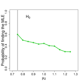
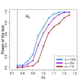
Figure 6: A demonstration of the validity of the two-sample test. The two samples are generated from two 3-Gaussian mixture models where the second center $\mu_{2}$ varies under different scenarios (when $\mu_{2}=0.75$, they are the same). We fit a 2-Gaussian mixture model to this problem. The left panel shows the chance of finding the MLE with a single random initialization when we combine two samples (Step 2 and 3 of Algorithm 3 of the main paper with $M=1$). The right panel shows the power curve of the proposed two-sample test under different significance level. In the case of $\mu_{2}=0.75$, we only have a chance of around 60% of finding the MLE but the two-sample test still maintain the type-I error properly. In both panels, the gray vertical line indicates where $H_{0}$ is true.

In Figure 6, we display a simulation result showing the power of the two-sample test under a Gaussian mixture model. The two samples are generated from univariate 3-Gaussian mixtures with

$$p_{1}(x) =0.5\phi(x;0,0.2^{2})+0.45\phi(x;0.75,0.2^{2})+0.05\phi(x;3,0.2^{2})$$

$$p_{2}(x) =0.5\phi(x;0,0.2^{2})+0.45\phi(x;\mu_{2},0.2^{2})+0.05\phi(x;3,0.2^{2}),$$

where $\phi(x;\mu,\sigma^{2})$ is the normal density with mean $\mu$ and variance $\sigma^{2}$. We generate $n_{1}=n_{2}=500$ observations in both samples. The only difference between the two samples is the second center $\mu_{2}$ in the second sample. We fit a 2-Gaussian mixture model to them with only one random initialization; in this case, there are multiple local modes in the likelihood space (part of the likelihood space can be seen in Figure 1). The left panel of Figure 6 shows the probability of finding the MLE under different $\mu_{2}$ (Step 2 and 3 of Algorithm 3 of main paper with $M=1$). The right panel of Figure 6 shows the power curve using the proposed two-sample test when the test statistic is the $L_{2}$ norm difference of the two fitted mean vectors. When $\mu_{2}=0.75$ ($H_{0}$ is true), there are only around 60% chance that we are using the MLE but our test still controls the type-I error properly.

Appendix B Future Work

B.1 Basins of Attraction of the EM-algorithm

In Section 4, we analyzed the performance of the EM-algorithm. However, the bound we obtain in Theorem 8 is very conservative because we only use a small ball within the basin of attraction of $\widehat{\theta}_{MLE}$, not the entire basin. Thus, a direction for future research is to investigate the basins of attraction of stationary points of an EM algorithm. In particular, we need to investigate how basins change under a small perturbation on the log-likelihood function (or its derivatives). With such stability result we could then obtain a refined bound on $P(\widehat{\theta}^{EM}_{n,M}=\widehat{\theta}_{MLE})$ and the loss of coverage.

B.2 High-dimensional Problems

Another direction for future work is to extend our framework to a high-dimensional M-estimator with a non-concave objective function (Loh and Wainwright, 2015; Loh, 2017; Elsener and van de Geer, 2018). Essentially, the log-likelihood function can be replaced by a loss function and the estimator $\widehat{\theta}_{MLE}$ becomes an M-estimator of an objective function.

The challenges in this generalization are the assumptions. Assumption (A3) in Appendix is not an issue because the uniform convergence of the gradient and the Hessian were proved in Mei et al. (2018). However, the constants in assumptions (A1), (A2), and (A4) may depend on the dimension and they could drastically reduce the convergence rate.

B.3 Stochastic Algorithms

Stochastic gradient ascent/descent (SGD; Kushner and Yin 2003; Bottou 2010; Pensia et al. 2018) and stochastic gradient Langevin dynamics (SGLD; Gelfand and Mitter 1991; Teh et al. 2016; Raginsky et al. 2017) are popular optimization techniques that can also be applied to find the MLE. A possible direction for future research is to study the estimators from SGD or SGLD using the analysis done in this paper. When using a stochastic algorithm, we introduce additional randomness into our estimator, contributing to a new source of uncertainty. But this uncertainty is based on our design, so we may be able to modify the CIs to account for this uncertainty. Thus, in principle we should be able to construct a CI with properties similar to those in Theorems 6 and 7. Note that Liang and Su (2019) have already analyzed the stochastic behavior of an estimator around a local optimum in a SGD method. Their results could be very useful in analyzing the uncertainty from a stochastic algorithm.

Appendix C Morse Theory

We summarize some useful results from Morse theory (Milnor, 1963; Morse, 1925, 1930) that are relevant to our analysis. Note that the notations in this section is self-consistent and should not be confused with the notations in other sections. For simplicity, we consider a function $f:{\mathbb{K}}\rightarrow{\mathbb{R}}$, where ${\mathbb{K}}\subset{\mathbb{R}}^{d}$ is a compact set.

A function $f$ is called a Morse function if all its critical points (points with $0$ gradient) are non-degenerate. When $f$ is at least twice differentiable, being a Morse function implies that all eigenvalues of its Hessian matrix at every critical point are non-zero.

Let $g=\nabla f$ and $H=\nabla\nabla f$ denote the gradient and Hessian matrix of $f$, respectively. Let ${\mathcal{C}}$ be the collection of critical points of $f$. For any point $x\in{\mathbb{K}}$, define a gradient flow $\gamma_{x}:{\mathbb{R}}\rightarrow{\mathbb{K}}$ such that

$$\gamma_{x}(0)=x,\quad\gamma_{x}^{\prime}(t)=g(\gamma_{x}(t)).$$

That is, $\gamma_{x}$ is a flow starting at point $x$ that moves according to the gradient of $f$. Then the Morse theory states that the destination

$$\gamma_{x}(\infty)=\lim_{t\rightarrow\infty}\gamma_{x}(t)$$

must be one of the critical points.

For a critical point $c\in{\mathcal{C}}$, define the basin of attraction ${\mathcal{A}}(c)=\{x:\gamma_{x}(\infty)=c\}$. The stable manifold theorem (see, e.g., Theorem 4.15 in Banyaga and Hurtubise 2013) shows that the basin ${\mathcal{A}}(c)$ is a $k$-dimensional manifold if $H(c)$ has $k$ negative eigenvalues. Namely, the basin of attraction of a local maximum is a $d$-dimensional manifold.

Let ${\mathcal{C}}_{j}$ denote the collection of all critical points with $j$ negative eigenvalues. Then, ${\mathcal{C}}_{d}$ is the collection of all local maxima and ${\mathcal{C}}_{0}$ is the collection of all local minima. Define

$${\mathcal{W}}_{j}=\bigcup_{c\in{\mathcal{C}}_{j}}{\mathcal{A}}(c).$$

to be the union of basins of attraction of critical points in ${\mathcal{C}}_{j}$. Then ${\mathcal{W}}_{0},\cdots,{\mathcal{W}}_{d}$ form a partition of ${\mathbb{K}}$. Namely,

$${\mathbb{K}}={\mathcal{W}}_{0}\cup{\mathcal{W}}_{1}\cup\cdots\cup{\mathcal{W}}_{d},\quad{\mathcal{W}}_{j}\cap{\mathcal{W}}_{\ell}=\emptyset\mbox{ for all }j\neq\ell.$$

Because ${\mathcal{W}}_{j}$ is the union of finite number of $j$-dimensional manifolds,

$$\mu({\mathcal{W}}_{j})=0,\quad j=0,\cdots,d-1,$$

where $\mu$ is the Lebesgue measure in ${\mathbb{R}}^{d}$.

The quantity ${\mathcal{W}}_{d}$ and its boundary are crucial in our analysis because ${\mathcal{W}}_{d}$ is the union of basins of attraction of local modes and is the only set within $\{{\mathcal{W}}_{j}:j=1,\cdots,d\}$ with a non-zero Lebesgue measure. Using the fact that ${\mathcal{W}}_{0},\cdots,{\mathcal{W}}_{d}$ form a partition of ${\mathbb{K}}$, the boundary of ${\mathcal{W}}_{d}$, denoted by ${\mathcal{B}}=\partial{\mathcal{W}}_{d}$, can be written as

$${\mathcal{B}}={\mathcal{W}}_{0}\cup{\mathcal{W}}_{1}\cup\cdots\cup{\mathcal{W}}_{d-1}.$$

Therefore, every point $x\in{\mathcal{B}}$ belongs to the basin of attraction of a critical point in ${\mathcal{C}}_{0}\cup{\mathcal{C}}_{1}\cup\cdots\cup{\mathcal{C}}_{d-1}$. Using the stable manifold theorem, $x$ is on a $k$-dimensional manifold, where $k$ is the number of negative eigenvalues of $H(\gamma_{x}(\infty))$. Thus, there is a well-defined normal space of $x$ relative to the manifold it falls within. We define $\mathcal{N}(x)$ to be the normal space of that manifold at point $x$. If $x\in{\mathcal{W}}_{k}$, we can find $d-k$ orthonormal vectors that span $\mathcal{N}(x)$. Let $v_{1},\cdots,v_{d-k}$ be an orthonormal basis of $\mathcal{N}(x)$ and define the matrix $V(x)=[v_{1},\cdots v_{d-k}]\in{\mathbb{R}}^{d\times(d-k)}$. We can then define the Hessian of $f$ in the normal space using $v_{1},\dots,v_{d-k}$ as

$$H_{V}(x)=V(x)^{T}H(x)V(x)\in{\mathbb{R}}^{(d-k)\times(d-k)}.$$ (13)

Namely, $H_{V}(x)$ is the Hessian matrix of $f$ by taking derivatives along $v_{1},\cdots,v_{d-k}$.

For a square matrix $M$, denote $\lambda_{|\min|}(M)$ as the smallest eigenvalue of $M$ in absolute value. The quantity

$$\rho(x)=\lambda_{|\min|}(H_{V}(x))=\inf_{v\in\mathcal{N}(x)}\frac{|v^{T}H(x)v|}{\|v\|^{2}}$$ (14)

plays a key role in controlling the stability of ${\mathcal{B}}$. Note that $\rho(x)$ is the smallest absolute eigenvalues of $H_{V}(x)$ so it is invariant of the orthonormal basis we are using. Later in assumption (A2) in Section D.1, we need $\inf_{x\in{\mathcal{B}}}\rho(x)\geq\rho_{\min}>0$. This assumption implies the stability of ${\mathcal{B}}$ (see Lemma 12). The quantity $\rho(x)$ also appears in Chen et al. (2017), where the authors used it to study the stability of the boundary of basins of attraction of a smooth density function.

When $d=1$, there are only two types of critical points – local minima and maxima – and the boundary ${\mathcal{B}}$ is the collection of local minima. Thus, $\rho(x)$ in equation (14) is just the absolute value of the second derivative at local minima and $\rho(x)>0$ is a necessary condition for $f$ to be a Morse function.

Appendix D Technical assumptions

D.1 Assumptions in Section 2.2

Let ${\mathcal{B}}=\bigcup_{\ell=1}^{K}\partial{\mathcal{A}}(m_{\ell})$ be the union of boundaries of basins of attraction of local maxima. The Morse theory implies that

$${\mathcal{B}}={\mathcal{W}}_{0}\cup{\mathcal{W}}_{1}\cup\cdots\cup{\mathcal{W}}_{d-1},$$

where ${\mathcal{W}}_{j}$ is a $j$-dimensional manifold (see Appendix C for more details). Namely, the boundary can be written as the union of basins of attraction of saddle points and local minima. Thus, every point $x\in{\mathcal{B}}$ admits a subspace space $\mathcal{N}(x)$ that is normal to ${\mathcal{B}}$ at $x$.

Assumptions.

• The (global) maximum is unique and there exist constants $g_{0},r_{0},\lambda_{0}>0$ such that:

  • At every critical point (i.e., $c:\nabla L(c)=0$), the eigenvalues of the Hessian matrix of $L(c)$ are outside $[-\lambda_{0},\lambda_{0}]$, and

  • for any $g<g_{0}$, there exists $r<r_{0}$ such that

    $$\{\theta:\|\nabla L(\theta)\|\leq g\}\subset\mathbb{C}\oplus r,$$

    where $\mathbb{C}=\{\theta:\nabla L(\theta)=0\}$ is the collection of all critical points.

• There exist $R_{1}>0$ and an integrable function $f(x)$ such that for every $i,j,k=1,\cdots,d$,

  $$\frac{\partial^{3}L(\theta|x)}{\partial\theta_{i}\partial\theta_{j}\partial\theta_{k}}\leq f(x)\quad\mbox{for all }\theta\in\mathcal{C}\oplus R_{1}.$$

  Moreover, there exists $\rho_{\min}>0$ such that

  $$\sup_{x\in{\mathcal{B}}}\inf_{v\in\mathcal{N}(x)}\frac{|v^{T}H(x)v|}{\|v\|^{2}}\geq\rho_{\min},$$

  where $\mathcal{N}(x)$ is the normal space of ${\mathcal{B}}$ at point $x$.

• Define

  $$\epsilon_{1,n} =\sup_{\theta\in\Theta}\left\|\nabla\widehat{L}_{n}(\theta)-\nabla L(\theta)\right\|_{\max},$$

  $$\epsilon_{2,n} =\sup_{\theta\in\Theta}\left\|\nabla\nabla\widehat{L}_{n}(\theta)-\nabla\nabla L(\theta)\right\|_{\max},$$

  where $\|\cdot\|_{\max}$ is the max-norm for a vector or a matrix. We need $\epsilon_{1,n},\epsilon_{2,n}=o(1)$ or $=o_{P}(1)$.

• There exists $r_{1}>0$ such that

  $$\epsilon_{3,n} =\max_{\ell=1,\cdots,K}\left|\widehat{\Pi}_{n}({\mathcal{A}}_{\ell})-\Pi({\mathcal{A}}_{\ell})\right|$$ (15)

  $$\epsilon_{4,n} =\sup_{r_{1}>r>0}\left|\widehat{\Pi}_{n}({\mathcal{B}}\oplus r)-\Pi({\mathcal{B}}\oplus r)\right|,$$ (16)

  $$\sup_{r_{1}>r>0}\Pi({\mathcal{B}}\oplus r) =O(r)$$ (17)

  with $\epsilon_{3,n},\epsilon_{4,n}=o(1)$ or $=o_{P}(1)$, where $\mathcal{A}_{\ell}\equiv\mathcal{A}(m_{\ell})$ for a local maximum $m_{\ell}\in\mathcal{C}$.

Assumption (A1) is called the strongly Morse assumption in Mei et al. (2018), and is often used in the literature to ensure critical points are well separated (Chazal et al., 2017; Genovese et al., 2016; Chen et al., 2016, 2017). Under assumption (A1), the likelihood function is a Morse function (Milnor, 1963; Morse, 1925).

Assumption (A2) consists of two parts: a third-order derivative assumption and a boundary curvature assumption. The third-order derivative assumption is a classical assumption to establish asymptotic normality (Redner and Walker, 1984; Van der Vaart, 1998). The boundary curvature assumption (Chen et al., 2017) assumes that when we are moving away from the boundary of a basin of attraction, the log-likeihood function has to behave like a quadratic function. When $d=1$, the boundary becomes the collection of local minima so this assumption reduces to requiring the second derivative is non-zero at local minima, which is a common assumption to ensure non-degenerate critical points.

Assumption (A3) requires that both the gradient and the Hessian can be uniformly estimated. It is also a common assumption in the literature, see, e.g., Genovese et al. (2016); Chazal et al. (2017); Mei et al. (2018); Chen et al. (2017).

The assumptions in (A4) are more involved. At first glance, it seems that the bound in equation (16) will be difficult to verify. However, there is a simple rule to verify it using the fact that the collection $\{{\mathcal{B}}\oplus r:r_{1}>r>0\}$ has VC dimension $1$ so as long as the convergence of $\widehat{\Pi}_{n}$ toward $\Pi$ can be written as an empirical process, this condition holds due to the VC theory (see Theorem 2.43 of Wasserman 2006). The assumption on the bound in equation (17) is required to avoid any probability mass around the boundary.

Here we gave additional assumptions on the likelihood function to obtain a concrete rate. Let $S(\theta|x)=\nabla L(\theta|x)$, and $H(\theta|x)=\nabla\nabla L(\theta|x)$, where the operator $\nabla$ is taking the gradient with respect to $\theta$.

Assumptions.

• The gradient and Hessian of the log-likelihood function are Lipschitz in the maximum norm in the following sense: there exist $m_{S}(x)$ and $m_{H}(x)$ with ${\mathbb{E}}(m^{2}_{S}(X_{1})),{\mathbb{E}}(m^{2}_{H}(X_{1}))<\infty$ such that for every $\theta_{1},\theta_{2}\in\Theta$,

  $$\|S(\theta_{1}|x)-S(\theta_{2}|x)\|_{\max} \leq m_{S}(x)\|\theta_{1}-\theta_{2}\|,$$

  $$\|H(\theta_{1}|x)-H(\theta_{2}|x)\|_{\max} \leq m_{H}(x)\|\theta_{1}-\theta_{2}\|.$$

• The quantities $\epsilon_{3,n},\epsilon_{4,n}$ in Assumption (A4) satisfy

  $$P\left(\max\{\epsilon_{3,n},\epsilon_{4,n}\}>t\right)\leq A_{1}n^{\nu}e^{-A_{2}nt^{2}},$$

  for some constants $A_{1},A_{2},\nu>0$.

Assumption (A3L) is a sufficient condition to ensure that we have a uniform concentration inequality of both the gradient and the Hessian. The Lipschitz condition is to guarantee that the parametric family has an $\epsilon$-bracketing number scaling at rate $O(\epsilon^{-d})$, where $d$ is the dimension of parameters (Van der Vaart, 1998). The bounds on the bracketing number can further be inverted into a concentration inequality using Talagrand’s inequality (see Theorem 1.3 of Talagrand 1994) Furthermore, (A3L) is a mild assumption because many common models, such as a Gaussian mixture model, satisfy this assumption when $\Theta$ is defined properly.

The concentration inequality assumption of (A4L) is also mild. The assumption is true whenever the data-driven approach $\widehat{\Pi}_{n}$ is based on fitting a smooth model such as a normal distribution on the parameter space with mean and variance being estimated by the data.

D.2 Assumptions in Section 3

Assumptions.

• The score function satisfies

  $${\mathbb{E}}\left(\|\nabla L(\theta|X_{1})\|^{4}\right)<\infty.$$

• There exist constants $R_{0},T_{0},T_{1}>0$ such that for every $\theta\in\mathcal{C}\oplus R_{0}$,

  $$\|\nabla\nabla\tau(\theta)\|_{\max} \leq T_{0}<\infty$$

  $$\|\nabla\tau(\theta)\| \geq T_{1}>0.$$

Assumption (A5) is related to but stronger than the assumption required by the Berry-Esseen bound (Berry, 1941; Esseen, 1942). We need the existence of the fourth-moment because we need a $\sqrt{n}$ convergence rate of the sample variance toward the population variance. It could be replaced by a third-moment assumption but in that case, we would not be able to obtain the convergence rate of the coverage of a CI. Assumption (T) ensures that the mapping $\tau(\cdot)$ is smooth around critical points so that we can apply the delta method (Van der Vaart, 1998) to construct a CI.

D.3 Assumptions in Section 4

Define $q(\theta)=Q(\theta|\theta_{MLE})$ and $\widehat{q}(\theta)=\widehat{Q}_{n}(\theta|\widehat{\theta}_{MLE})$. Let $\nabla_{\omega}$ be taking gradient with respect to the variable $\omega$ and

$${\mathcal{A}}^{EM}(\theta_{MLE})=\{\theta^{(0)}:\theta^{(\infty)}=\theta_{MLE}\}$$

be the basin of attraction of $\theta_{MLE}$.

Assumptions.

• $\theta_{MLE}$ is the unique maximizer of $q(\theta)$.

• There exists a positive number $r_{0}>0$ such that the following two conditions are met:

  • There is a positive number $\lambda_{0}>0$ that

    $$\sup_{\theta\in B(\theta_{MLE},r_{0})}\lambda_{\max}\left(\nabla\nabla q(\theta)\right)\leq-\lambda_{0}<0,$$

    where $\lambda_{\max}(A)$ is the largest eigenvalue of matrix $A$.

  • There is a positive number $\kappa_{0}<\lambda_{0}$ such that

    $$\sup_{\theta,\theta^{\prime}\in B(\theta_{MLE},r_{0})}\left\|\nabla_{\theta}\nabla_{\theta^{\prime}}Q(\theta|\theta^{\prime})\right\|\leq\kappa_{0}.$$

• Let $H_{q}(\theta|\theta^{\prime},x)=\nabla_{\theta}\nabla_{\theta^{\prime}}Q(\theta|\theta^{\prime},x)$ and $H_{q}(\theta|x)=\nabla_{\theta}\nabla_{\theta}Q(\theta|\theta_{MLE},x)$. There exist $m_{\theta\theta}(x)$ and $m_{q\theta}(x)$ with ${\mathbb{E}}(m^{2}_{\theta\theta}(X_{1})),{\mathbb{E}}(m^{2}_{q\theta}(X_{1}))<\infty$ such that for any $\theta_{1},\theta_{2}\in B(\theta_{MLE},r_{0})$,

  $$\sup_{\theta^{\prime}\in B(\theta_{MLE},r_{0})}\|H_{q}(\theta^{\prime}|\theta_{1},x)-H_{q}(\theta^{\prime}|\theta_{2},x)\|_{\max} \leq m_{\theta\theta}(x)\|\theta_{1}-\theta_{2}\|$$

  $$\|H_{q}(\theta_{1}|x)-H_{q}(\theta_{2}|x)\|_{\max} \leq m_{q\theta}(x)\|\theta_{1}-\theta_{2}\|,$$

  where $r_{0}$ is the constant in (EM2).

• Let $r_{0}$ be the constant in (EM2). For each $t>0$, there exists a function $\eta_{n}(t)$ such that

  $$P\left(\left|\widehat{\Pi}_{n}\left(B\left(\theta_{MLE},\frac{r_{0}}{3}\right)\right)-\Pi\left(B\left(\theta_{MLE},\frac{r_{0}}{3}\right)\right)\right|>t\right)<\eta_{n}(t)$$

  and $\eta_{n}(t)=o(1)$ when $n\rightarrow\infty$.

Assumption (EM1) is known as the self-consistency property (Dempster et al., 1977; Balakrishnan et al., 2017), and it is a very common condition used to establish the stability of the EM algorithm around the population MLE. Assumption (EM2) regularizes the behavior of $q$ and $Q$ around the MLE. In a sense, (EM2-1) requires that the function $q$ is quadratic around the MLE; this further implies the strongly concavity assumption in Balakrishnan et al. (2017). (EM2-2) requests that the function $Q(\theta|\theta^{\prime})$ changes smoothly when varying $\theta$ or $\theta^{\prime}$ which, when being satisfied, implies the first-order stability assumption in Balakrishnan et al. (2017). Assumption (EM3) is related to the concentration inequalities for approximating $q(\theta)$ and $Q(\theta|\theta^{\prime})$ by their empirical versions $\widehat{q}(\theta)$ and $\widehat{Q}(\theta|\theta^{\prime})$. This assumption can be viewed as a modified version of the assumption (A3L). The final assumption (EM4) is related to assumptions (A4L) but it is much weaker – we only need to focus on the probability of a ball around the MLE. In many cases, $\eta_{n}(t)=A_{1}e^{-A_{2}nt^{2}}$ for some positive constants $A_{1}$ and $A_{2}$.

D.4 Assumptions of Appendix E

Let $\beta=(\beta_{1},\cdots,\beta_{d})\in\{0,1,2,\cdots\}^{d}$ be a multi-index variable with $d$ variables and $\|\beta\|_{1}=\sum_{j=1}^{d}\beta_{j}$. For a multivariate function $f$ with $d$ arguments (i.e., $f:{\mathbb{R}}^{d}\mapsto{\mathbb{R}}$), we define

$$f^{(\beta)}(x)=\frac{\partial^{\|\beta\|_{1}}}{\partial x_{1}^{\beta_{1}}\cdots\partial x_{d}^{\beta_{d}}}f(x).$$

Namely, $f^{(\beta)}$ is taking derivatives with respect to the coordinate corresponding to $\beta$. Let $\mathbf{BC}^{r}$ denote the collection of functions with bounded continuous derivatives up to the $r$-th order. We consider the following two common assumptions on the kernel function:

• The kernel function $K\in\mathbf{BC}^{3}$ and is symmetric, non-negative, and

  $$\int x^{2}K^{(\beta)}(x)dx<\infty,\qquad\int\left(K^{(\beta)}(x)\right)^{2}dx<\infty$$

  for all $\|\beta\|_{1}=0,1,2,3$.

• The kernel function satisfies condition $K_{1}$ (VC-subgraph condition) of Gine and Guillou (2002). That is, there exist some $A,\nu,C_{K}>0$ such that for all $0<\epsilon<1$, we have $\sup_{Q}N(\mathcal{K},L_{2}(Q),C_{K}\epsilon)\leq\left(\frac{A}{\epsilon}\right)^{\nu},$ where $N(\mathcal{K},d,\epsilon)$ is the $\epsilon$-covering number for a semi-metric space $(\mathcal{K},d)$, and

  $$\mathcal{K}=\Biggl{\{}u\mapsto K^{(\beta)}\left(\frac{x-u}{h}\right):x\in{\mathbb{R}}^{d},h>0,\|\beta\|_{1}=0,1,2\Biggr{\}}$$

  and $C_{K}=\sup_{f\in\mathcal{K}}\|f\|_{\infty}$. Namely, $\mathcal{K}$ is the collection of kernel functions and their partial derivatives up to the second order.

Assumption (K1) is a common assumption used to obtain the convergence rate of a KDE; see Wasserman (2006). Assumption (K2) is a mild assumption that establishes uniform convergence of the KDE and its derivatives. It first appeared in Gine and Guillou (2002) and Einmahl and Mason (2005) and is a common assumption in the literature; for examples, see Genovese et al. (2014); Chen et al. (2015); Genovese et al. (2016)

The assumption of (K1) and (K2) implies the following concentration inequality.

Lemma 10 (Talagrand’s inequality for KDE and its derivatives).

Assume (K2) and that ${\mathbb{K}}$ is a compact set and $h\rightarrow 0$, $n\rightarrow\infty$, $\frac{nh^{d+4}}{\log n}\rightarrow\infty$. Let $\widehat{p}_{h}(x)$ be the KDE and $\widehat{g}_{h}(x)$ be its gradient and $\widehat{H}_{h}(x)$ be the Hessian matrix. Then there exist positive numbers $A_{1},A_{2}$, and $t_{0}$ such that

$$P\left(\sup_{x\in{\mathbb{K}}}\|\widehat{p}_{h}(x)-{\mathbb{E}}(\widehat{p}_{h}(x))\|>t\right) \leq A_{1}e^{-A_{2}nh^{d}t^{2}}$$

$$P\left(\sup_{x\in{\mathbb{K}}}\|\widehat{g}_{h}(x)-{\mathbb{E}}(\widehat{g}_{h}(x))\|_{\max}>t\right) \leq A_{1}e^{-A_{2}nh^{d+2}t^{2}}$$

$$P\left(\sup_{x\in{\mathbb{K}}}\|\widehat{H}_{h}(x)-{\mathbb{E}}(\widehat{H}_{h}(x))\|_{\max}>t\right) \leq A_{1}e^{-A_{2}nh^{d+4}t^{2}}$$

for every $t>\frac{t_{0}}{\sqrt{n}}.$

As this lemma is a direct result from Theorem 1.1 of Talagrand (1994) and assumption (K2), we omit the proof.

Appendix E Nonparametric Mode Hunting

To demonstrate that our analysis can be applied to situations outside the likelihood model, we study the nonparametric mode hunting problem. Mode hunting aims to find the global mode/maximum (or all local modes) of the underlying probability density function (Good and Gaskins, 1980; Hall et al., 2004; Burman and Polonik, 2009). This is a classical problem in density estimation (Parzen, 1962; Romano, 1988a, b) and is often related to the task of clustering (Li et al., 2007; Azizyan et al., 2015; Chacón et al., 2015; Chen et al., 2016). In this section, we focus on inferring the global mode.

We assume that our data consists of $X_{1},\cdots,X_{n}$ that are IID from an unknown PDF $p$ with a compact support ${\mathbb{K}}\subset{\mathbb{R}}^{d}$. The goal is to make inference of ${\sf Mode}(p)={\sf argmax}_{x\in{\mathbb{K}}}\,\,p(x).$

A plug-in estimate from a density estimator offers a simple approach of finding the mode. Namely, we first construct a smooth density estimator $\widehat{p}_{h}$ using the data and then form our estimator $\widehat{\sf Mode}(p)={\sf Mode}(\widehat{p}_{h}).$ A popular choice of $\widehat{p}_{h}$ is the kernel density estimator (KDE): $\widehat{p}_{h}(x)=\frac{1}{nh^{d}}\sum_{i=1}^{n}K\left(\frac{X_{i}-x}{h}\right),$ where $K(\cdot)$ is a smooth function called the kernel function (we often use the Gaussian as the kernel) and $h>0$ is the smoothing bandwidth that controls the amount of smoothing.

When using a KDE to do mode hunting, there is a simple numerical approach called the meanshift algorithm (Cheng, 1995; Comaniciu and Meer, 2002; Fukunaga and Hostetler, 1975). The meanshift algorithm is a gradient ascent method that moves a given point $x_{0}$ by its density gradient $\nabla\widehat{p}_{h}(x_{0})$ until it arrives at a local mode. Specifically, given a point $x_{t}$, the meanshift algorithm moves it to

$$x_{t+1}\leftarrow\frac{\sum_{i=1}^{n}X_{i}K\left(\frac{X_{i}-x_{t}}{h}\right)}{\sum_{i=1}^{n}K\left(\frac{X_{i}-x_{t}}{h}\right)}.$$

One can show that the amount of shift, $x_{t+1}-x_{t}$, is proportional to the gradient $\nabla\widehat{p}_{h}(x_{t})$ when the kernel function $K$ is the Gaussian. This implies that the meanshift algorithm is a gradient ascent approach.

Although there are many ways of choosing the initial points, we consider a simple method through which we generate $n$ initial points by sampling with replacement from the observed data points. This implies that $M=n$ and $\widehat{\Pi}_{n}=\widehat{P}_{n},$ where $\widehat{P}_{n}$ is the empirical distribution function. This method is based on the fact that the density around the mode is often very high, so it is very likely to have observations within the basin of attraction of the mode. After $n$ initializations, let $\widehat{\sf Mode}^{\dagger}(p)$ denote the resulting estimator of the mode. We will use $\widehat{\sf Mode}^{\dagger}(p)$ to construct a CI.

Because the asymptotic covariance matrix of the mode estimator $\widehat{\sf Mode}^{\dagger}(p)$ is quite complex, we use the bootstrap approach. Let $X^{*}_{1},\cdots,X^{*}_{n}$ be a bootstrap sample (from sampling the original dataset with replacement) and $\widehat{p}_{h}^{*}$ be the corresponding KDE using the same smoothing bandwidth and the same kernel function. Using the estimator $\widehat{\sf Mode}^{\dagger}(p)$ as the initial point, we apply the meanshift algorithm with the bootstrap sample $X^{*}_{1},\cdots,X^{*}_{n}$ and iterate it until the algorithm convergence. Let $\widehat{\sf Mode}^{\dagger*}(p)$ be the convergent point, which can be viewed as the mode estimator using the bootstrap sample. Let $\widehat{d}^{\dagger}_{1-\alpha}$ be the $1-\alpha$ quantile of $\left\|\widehat{\sf Mode}^{\dagger*}(p)-\widehat{\sf Mode}^{\dagger}(p)\right\|$ given $X_{1},\cdots,X_{n}$. Namely,

$$\widehat{d}^{\dagger}_{1-\alpha} =\widehat{G}^{-1}_{h}(1-\alpha),$$

$$\widehat{G}_{h}(t) =P\left(\left\|\widehat{\sf Mode}^{\dagger*}(p)-\widehat{\sf Mode}^{\dagger}(p)\right\|<t|X_{1},\cdots,X_{n}\right).$$

Define a $1-\alpha$ CI as $\mathbb{M}_{n,\alpha}=\left\{x:\left\|x-\widehat{\sf Mode}^{\dagger}(p)\right\|\leq\widehat{d}^{\dagger}_{1-\alpha}\right\}.$ Namely, $\mathbb{M}_{n,\alpha}$ is a ball centered at the original estimator $\widehat{\sf Mode}^{\dagger}(p)$ with a radius $\widehat{d}^{\dagger}_{1-\alpha}$.

Theorem 11.

Assume (A1) and (A2) in Appendix D.1 of the density function and also that the kernel function satisfies assumptions (K1) and (K2) in Appendix D.4. Suppose $h\rightarrow 0$, $\frac{nh^{d+4}}{\log n}\rightarrow\infty$, and $nh^{d+6}\rightarrow 0$, then

$$P(\mathbb{M}_{n,\alpha}\cap{{\mathcal{C}}}_{n,\delta}^{\pi}\neq\emptyset) \geq 1-\alpha-\delta-O\left(\sqrt{nh^{d+6}}\right)-O\left(\sqrt{\frac{\log n}{nh^{d+2}}}\right),$$

where ${{\mathcal{C}}}_{n,\delta}^{\pi}$ is the set defined in Section 2.1 from replacing the likelihood function $L$ and initialization distribution $\Pi$ by $p$ and $P$, respectively. Moreover, let $\mathcal{A}_{\sf mode}$ denote the basin of attraction of the mode of $p$. Then under the same requirement for the smoothing bandwidth,

$$P({\sf Mode}(p)\in\mathbb{M}_{n,\alpha}) \geq 1-\alpha-\left(1-\frac{1}{3}P(\mathcal{A}_{\sf mode})\right)^{n}-O\left(\sqrt{nh^{d+6}}\right)-O\left(\sqrt{\frac{1}{nh^{d+2}}}\right).$$

Theorem 11 is analogous to Theorem 7 where the two big-O terms are generated from the bias and the stochastic variation of a nonparametric estimator. The quantity $\left(1-\frac{1}{3}P(\mathcal{A}_{\sf mode})\right)^{n}$ in the second assertion is needed to account for the uncertainty from initializations. The multiplier $\frac{1}{3}$ is a constant that we use to simplify the proof and it can be improved to any fixed number that is less than $1$ (we cannot replace it by $1$ due to the uncertainty of the basin of attraction and the uncertainty of initialization method). Asymptotically, this quantity can be ignored because it is exponentially converging to $0$; we keep it here to emphasize the uncertainty from initializations. The fact that this quantity is much smaller than the other components, $O\left(\sqrt{nh^{d+6}}\right)$ and $O\left(\sqrt{\frac{1}{nh^{d+2}}}\right)$, implies that in nonparametric mode hunting, the main bottleneck for the coverage is not from initialization but from the nonparametric estimation of the gradient. Note that the big-O terms in the first and the second assertions differ by a $\sqrt{\log n}$ term ($O\left(\sqrt{\frac{\log n}{nh^{d+2}}}\right)$ versus $O\left(\sqrt{\frac{1}{nh^{d+2}}}\right)$). This discrepancy comes from the fact that the uncertainty of boundary in the first case introduces an error at the order of the uniform convergence rate of the gradient, which is $O\left(\sqrt{\frac{\log n}{nh^{d+2}}}\right)$. In the second case, the uncertainty of boundary is absorbed into the quantity $\frac{1}{3}P(\mathcal{A}_{\sf mode})$ and the rate $O\left(\sqrt{\frac{1}{nh^{d+2}}}\right)$ comes from the estimating the gradient of the density function.

We have two requirements on the smoothing bandwidth: $\frac{nh^{d+4}}{\log n}\rightarrow\infty$ and $nh^{d+6}\rightarrow 0$. The former condition ensures the uniform convergence of the Hessian matrix of the KDE. The latter one is an undersmoothing bandwidth requirement for gradient estimation. We need to undersmooth the gradient estimation so that the bias converges faster than the stochastic variation, leading to a CI with the desired coverage.

Theorem 11 is consistent with Theorem 2.1 of Romano (1988a), where the author proved that the empirical bootstrap leads to a consistent CI of the mode in $d=1$ when the smoothing bandwidth satisfies $nh^{7}\rightarrow 0,\frac{nh^{5}}{\log n}\rightarrow\infty$.

Theorem 11 is similar to Theorem 7 but there are two major differences. First, assumption (A3) holds with $\epsilon_{1,n}=O(h^{2})+O_{P}\left(\sqrt{\frac{\log n}{nh^{d+2}}}\right)$, $\epsilon_{2,n}=O(h^{2})+O_{P}\left(\sqrt{\frac{\log n}{nh^{d+4}}}\right)$. These are the nonparametric estimation rates of the gradient and Hessian matrix (see, e.g., page 17 of Genovese et al. 2014 and Lemma 10 of Chen et al. 2015). The other difference is that the CI here is in ${\mathbb{R}}^{d}$ so we need to apply a multivariate Berry-Esseen bound (Gotze, 1991; Sazonov, 1968). Note that the use of empirical measure for the initializations (i.e., $\widehat{\Pi}_{n}=\widehat{P}_{n}$) automatically implies that the assumption (A4L) holds.

Appendix F Uncertainty Analysis

As is discussed in the main paper, the behavior of the estimator $\widehat{\theta}_{n,M}$ depends on several components: the initialization method, the number of initializations, and the sample size. Each of these factors contribute to the uncertainties of $\widehat{\theta}_{n,M}$. In this section, we categorize the uncertainties based on their sources and discuss possible remedies to reduce them.

Source 1: Uncertainty of parameter estimation. The uncertainty of parameter estimation has been studied in the statistical literature for decades. This source of uncertainty is often captured by a CI or the standard error (McLachlan and Peel, 2004; McLachlan and Krishnan, 2007). Uncertainty of parameter estimation is caused by the random fluctuation of the estimated likelihood function around each local maximum. Under assumption (A1), this uncertainty is often related to the convergence rate of the gradient of the log-likelihood function (score function) because the local maxima (critical points) are where the gradient is $0$. Common CIs, such as the normal CI (Section 3.1) and the bootstrap CI (Section 3.2), can capture this type of uncertainty.

Source 2: Number of initializations. When the likelihood function has multiple local modes, initializations introduce uncertainties of $\widehat{\theta}_{n,M}$. Small number of initializations leads to a large uncertainty of $\widehat{\theta}_{n,M}$. There are two ways of expressing this type of uncertainty. First, from the analysis in Section 2, we know that the estimator $\widehat{\theta}_{n,M}$ is close to an element of ${{\mathcal{C}}}^{\pi}_{M,\delta}$ with a probability of at least $1-\delta$. Thus, for a given initialization method, the size of ${{\mathcal{C}}}^{\pi}_{M,\delta}$ can be a measure of the uncertainty related to the number of initializations. The other way of expressing this uncertainty is the loss in coverage of a CI with respect to covering $\tau_{MLE}$. In Theorem 6 and 7, we see that the probability of a CI of containing $\tau_{MLE}$ is $1-\alpha-(1-q^{\pi}_{1})^{M}$. The quantity $(1-q^{\pi}_{1})^{M}$ is the uncertainty caused by $M$, the number of initializations.

Source 3: Uncertainty of the initialization method. Another source of uncertainty in our inference comes from the differences between the data-driven initialization method $\widehat{\Pi}_{n}$ and its population version $\Pi$. At the population level, the set to which the estimator $\widehat{\theta}_{n,M}$ is converging, ${{\mathcal{C}}}^{\pi}_{M,\delta}$, is defined through the limiting initialization distribution $\Pi$. But our estimator $\widehat{\theta}_{n,M}$ is constructed by applying the gradient ascent with initializations from $\widehat{\Pi}_{n}$. Thus, the differences in initialization methods also contribute to the uncertainty in our inference. The first two requirements in assumption (A4) serve to regularize the uncertainty from this source.

Source 4: Uncertainty of the basin of attraction. An important quantity in the construction of ${{\mathcal{C}}}^{\pi}_{M,\delta}$ is the basin of attraction of gradient flows of $L$. When we compute the estimator $\widehat{\theta}_{n,M}$, the relevant basins of attraction are defined through gradient flows of $\widehat{L}_{n}$. Such basins of attraction are often different and the differences contribute uncertainty to our inference. Under assumptions (A2) and (A4), this uncertainty is controlled by the rate of estimating the gradient of the log-likelihood function.

Source 5: Algorithmic uncertainty. In this paper, we assumed that we can use the actual ‘continuous’ gradient ascent flow to find the estimator. However, in practice gradient ascent algorithms perform a ‘discrete’ gradient ascent, and thus the number of iterations and the step size used in the algorithm will affect the performance of the estimator. This type of uncertainty should also be considered when we report our findings. Fortunately, when the initial point is sufficiently close to a local optimum (so that the objective function is locally strongly concave/convex) and the step size is sufficiently small (both bounds are known in the literature–related to the conditioning number; Nesterov 2013), a gradient decent algorithm converges linearly to a critical point (Boyd and Vandenberghe, 2004; Nesterov, 2013). When the initial point is outside the nice area, it is less clear about how the gradient decent algorithm and the corresponding flow are related; some prior work can be found in Beyn (1987); Merlet and Pierre (2010); Arias-Castro et al. (2016). So this may introduce some additional uncertainties.

Appendix G Proofs

of Proposition 2.

Our proof consists of two parts. In the first part, we will prove that the likelihood function $L(\theta)$ is concave within the ball $B(\theta_{MLE},\frac{\lambda_{0}}{c_{3}})$ and conclude that $B(\theta_{MLE},\frac{\lambda_{0}}{c_{3}})\subset\mathcal{A}(\theta_{MLE})$. In the second part, we will derive the bound on $M$.

Part 1: Concavity of $L(\theta)$ within $B(\theta_{MLE},\frac{\lambda_{0}}{c_{3}})$. For any point $x\in B(\theta_{MLE},\frac{\lambda_{0}}{c_{3}})$, define $\omega=x-\theta_{MLE}$ and $\omega_{0}=\frac{\omega}{\|\omega\|}$. To show the concavity, we start with analyzing the Hessian matrix $H(x)$. By Taylor’s theory,

$$H(x)=H(\theta_{MLE}+\omega) =H(\theta_{MLE})+\int_{t=0}^{t=\|\omega\|}dH(\theta_{MLE}+t\omega_{0})$$

$$=H(\theta_{MLE})+\int_{t=0}^{t=\|\omega\|}\frac{dH(\theta_{MLE}+t\omega_{0})}{dt}dt$$

$$=H(\theta_{MLE})+\int_{t=0}^{t=\|\omega\|}\nabla_{\omega_{0}}H(\theta_{MLE}+t\omega_{0})dt,$$

where $\nabla_{\omega_{0}}$ denotes the directional derivative with respect to $\omega_{0}$. Thus,

$$\|H(x)-H(\theta_{MLE})\|_{2} =\left\|\int_{t=0}^{t=\|\omega\|}\nabla_{\omega_{0}}H(\theta_{MLE}+t\omega_{0})dt\right\|_{2}$$

$$\leq\int_{t=0}^{t=\|\omega\|}\left\|\nabla_{\omega_{0}}H(\theta_{MLE}+t\omega_{0})\right\|_{2}dt$$

$$\leq\int_{t=0}^{t=\|\omega\|}c_{3}dt$$

$$=c_{3}\|\omega\|\leq\lambda_{0}.$$

Note that we use the fact that $\|\omega\|=\|x-\theta_{MLE}\|\leq\frac{\lambda_{0}}{c_{3}}$ in the last inequality. By the Weyl’s inequality (see, e.g., Theorem 4.3.1 of Horn and Johnson 1990),

$$\lambda_{\max}(H(x))\leq\lambda_{\max}(H(\theta_{MLE}))+\|H(x)-H(\theta_{MLE})\|_{2}<-\lambda_{0}+\lambda_{0}=0,$$

where $\lambda_{\max}(A)$ is the largest eigenvalue of a square matrix $A$. Thus, every eigenvalue of $H(x)$ is negative so $H(x)$ is negative definite. This analysis applies to every $x\in B(\theta_{MLE},\frac{\lambda_{0}}{c_{3}})$. This, together with the fact that the ball $B(\theta_{MLE},\frac{\lambda_{0}}{c_{3}})$ is a convex set, implies that $L(\theta)$ is a concave function within $B(\theta_{MLE},\frac{\lambda_{0}}{c_{3}})$, which further implies that $B\left(\theta_{MLE},\frac{\lambda_{0}}{c_{3}}\right)\subset\mathcal{A}(\theta_{MLE})$.

Part 2: Bound the number $M$. Because $B(\theta_{MLE},\frac{\lambda_{0}}{c_{3}})\subset\mathcal{A}(\theta_{MLE})$,

$$q^{\pi}_{1}=\Pi(\mathcal{A}(\theta_{MLE}))\geq\Pi\left(B\left(\theta_{MLE},\frac{\lambda_{0}}{c_{3}}\right)\right)$$

To make sure ${{\mathcal{C}}}^{\pi}_{M,\delta}=\{\theta_{MLE}\}$, we need $M$ to satisfy

$$(1-q^{\pi}_{1})^{M}\leq\delta.$$

Thus, a lower bound on $M$ is

$$\left(1-\Pi\left(B\left(\theta_{MLE},\frac{\lambda_{0}}{c_{3}}\right)\right)\right)^{M}\leq\delta.$$

Taking logarithm in both sides, we obtain

$$M\cdot\log\left(1-\Pi\left(B\left(\theta_{MLE},\frac{\lambda_{0}}{c_{3}}\right)\right)\right)\leq\log\delta.$$

Because $\log\left(1-\Pi\left(B\left(\theta_{MLE},\frac{\lambda_{0}}{c_{3}}\right)\right)\right)$ is negative, so this is equivalent to

$$M\geq\frac{\log\delta}{\log\left(1-\Pi\left(B\left(\theta_{MLE},\frac{\lambda_{0}}{c_{3}}\right)\right)\right)},$$

which is the desired bound.

∎

Before proving Theorem 4, we first recall a useful result from Chen et al. (2017). For two sets $A$ and $B$, define their Hausdorff distance as

$$d_{H}(A,B)=\inf\{r>0:B\subset A\oplus r,\,\,A\subset B\oplus r\},$$

where $A\oplus r=\{x:\inf_{y\in A}\|x-y\|\leq r\}$ is the region within a distance $r$ to the set $A$. The Hausdorff distance can be viewed as an $L_{\infty}$ distance between sets.

Lemma 12 (Theorem 1 of Chen et al. (2017)).

Assume (A1–3) and $\max\{\epsilon_{1,n},\epsilon_{2,n}\}\rightarrow 0$. Let ${\mathcal{B}}$ be the boundary of basin of attraction defined in Section 2.2 and $\widehat{\mathcal{B}}$ be the corresponding sample version. Then

$$d_{H}(\mathcal{B},\widehat{\mathcal{B}})=O(\epsilon_{1,n}).$$

of Theorem 4.

We assume that Lemma 3 holds so that there exists $\bar{\theta}\in{{\mathcal{C}}}$ such that $\widehat{\theta}_{n,M}$ is closest to $\bar{\theta}$. Therefore, we can write $\|\widehat{\theta}_{n,M}-\bar{\theta}\|=d(\widehat{\theta}_{n,M},{{\mathcal{C}}})$ and focus on the analysis of $\|\widehat{\theta}_{n,M}-\bar{\theta}\|$. Note that by definition, Lemma 3 holds with a probability of $1-\xi_{n}$.

The proof of the first argument contains three steps (part 1-3). In the first step, we bound the distance $\|\widehat{\theta}_{n,M}-\bar{\theta}\|$. In the second step we analyze the difference between probabilities $\widehat{q}_{\ell}-q_{\ell}$. Then in the third step, we show that with some probability, $\bar{\theta}\in{{\mathcal{C}}}^{\pi}_{M,\delta}$. The first and third steps together imply a bound on $d(\widehat{\theta}_{n,M},{{\mathcal{C}}}^{\pi}_{M,\delta}),$ which is the desired quantity. The proof of the second argument will be in the part 4, which is built on the first three parts.

Recall that $S(\theta)=\nabla L(\theta)$, $H(\theta)=\nabla\nabla L(\theta)$, $\widehat{S}_{n}(\theta)=\nabla\widehat{L}_{n}(\theta)$, and $\widehat{H}_{n}(\theta)=\nabla\nabla\widehat{L}_{n}(\theta)$.

Step 1: bounding $\|\widehat{\theta}_{n,M}-\bar{\theta}\|$. Because $\widehat{\theta}_{n,M}$ is a local maximum of $\widehat{L}_{n}$ and $\bar{\theta}$ is a local maximum of $L$, we have

$$0=\widehat{S}_{n}(\widehat{\theta}_{n,M})=S(\bar{\theta}).$$

Thus, by Taylor expansion and the differentiability of $L$ in assumption (A2),

$$\widehat{S}_{n}(\bar{\theta})-S(\bar{\theta}) =\widehat{S}_{n}(\bar{\theta})-\widehat{S}_{n}(\widehat{\theta}_{n,M})$$

$$=\widehat{H}_{n}(\bar{\theta})(\bar{\theta}-\widehat{\theta}_{n,M})+O\left(\|\bar{\theta}-\widehat{\theta}_{n,M}\|^{2}\right)$$

$$=H^{-1}(\theta)\left(\bar{\theta}-\widehat{\theta}_{n,M}\right)+O\left(\|\bar{\theta}-\widehat{\theta}_{n,M}\|\cdot\epsilon_{2,n}+\|\bar{\theta}-\widehat{\theta}_{n,M}\|^{2}\right),$$

which implies

$$\widehat{\theta}_{n,M}-\bar{\theta} =-H^{-1}(\bar{\theta})(\widehat{S}_{n}(\bar{\theta})-S(\bar{\theta}))+O\left(\|\bar{\theta}-\widehat{\theta}_{n,M}\|\cdot\epsilon_{2,n}+\|\bar{\theta}-\widehat{\theta}_{n,M}\|^{2}\right).$$ (18)

Note that $\widehat{H}^{-1}_{n}(\bar{\theta})=H^{-1}(\bar{\theta})+O(\epsilon_{2,n})$ is due to assumption (A1) that the Hessian matrix is invertible around each neighborhood of local maxima.

Because $\|\widehat{S}_{n}(\bar{\theta})-S(\bar{\theta})\|\leq\sup_{\theta\in\Theta}\|\widehat{S}_{n}({\theta})-S({\theta})\|=\epsilon_{1,n}$, we conclude that

$$\widehat{\theta}_{n,M}-\bar{\theta}=d(\widehat{\theta}_{n,M},{{\mathcal{C}}})=O(\epsilon_{1,n}).$$

Step 2. Bounding the probability difference $\widehat{q}_{\ell}-q_{\ell}$. We will prove that $\widehat{q}_{\ell}-q_{\ell}=O(\epsilon_{1,n}+\epsilon_{3,n}+\epsilon_{4,n})$. Note that we assume that Lemma 3 holds throughout the entire proof so each $q_{\ell}$ corresponds to $\widehat{q}_{\ell}$ after relabeling. Recall that $q_{\ell}=\Pi(\mathcal{A}_{\ell})$ and $\widehat{q}_{\ell}=\widehat{\Pi}_{n}(\widehat{\mathcal{A}}_{\ell})$. By triangle inequality,

$$|\widehat{q}_{\ell}-q_{\ell}|=|\widehat{\Pi}_{n}(\widehat{\mathcal{A}}_{\ell})-\Pi(\mathcal{A}_{\ell})|\leq\underbrace{|\widehat{\Pi}_{n}(\widehat{\mathcal{A}}_{\ell})-\widehat{\Pi}_{n}(\mathcal{A}_{\ell})|}_{(I)}+\underbrace{|\widehat{\Pi}_{n}(\mathcal{A}_{\ell})-\Pi(\mathcal{A}_{\ell})|}_{(II)}.$$ (19)

Using the symmetric difference, $A\triangle B=(A\backslash B)\cup(B\backslash A)$, the first part (I) can be bounded by

$$(I) =|\widehat{\Pi}_{n}(\widehat{\mathcal{A}}_{\ell})-\widehat{\Pi}_{n}(\mathcal{A}_{\ell})|$$

$$\leq\widehat{\Pi}_{n}(\widehat{\mathcal{A}}_{\ell}\triangle\mathcal{A}_{\ell})$$

For any point $x\in\widehat{\mathcal{A}}_{\ell}\triangle\mathcal{A}_{\ell}$, this point must be within the set $\mathcal{B}\oplus d_{H}(\mathcal{B},\widehat{\mathcal{B}})$. Lemma 12 implies $d_{H}(\mathcal{B},\widehat{\mathcal{B}})=O(\epsilon_{1,n})$, so

$$\widehat{\mathcal{A}}_{\ell}\triangle\mathcal{A}_{\ell}\subset\mathcal{B}\oplus O(\epsilon_{1,n}).$$

By the second assertion of assumption (A4) and the fact that $\epsilon_{1,n}\rightarrow 0$,

$$\widehat{\Pi}_{n}(\widehat{\mathcal{A}}_{\ell}\triangle\mathcal{A}_{\ell})\leq\widehat{\Pi}_{n}(\mathcal{B}\oplus O(\epsilon_{1,n}))\leq\Pi(\mathcal{B}\oplus O(\epsilon_{1,n}))+O(\epsilon_{4,n}).$$

Moreover, the third assertion of assumption (A4) implies that $\Pi({\mathcal{B}}\oplus O(\epsilon_{1,n}))=O(\epsilon_{1,n})$. Therefore, we conclude that

$$(I)=O(\epsilon_{1,n}+\epsilon_{4,n}).$$

For the quantity (II), the first assertion in assumption (A4) directly shows that

$$(II)=|\widehat{\Pi}_{n}(\mathcal{A}_{\ell})-\Pi(\mathcal{A}_{\ell})|\leq\epsilon_{3,n}.$$

Putting it altogether, equation (19) implies

$$|\widehat{q}_{\ell}-q_{\ell}|\leq(I)+(II)=O(\epsilon_{1,n}+\epsilon_{3,n}+\epsilon_{4,n}).$$ (20)

Part 3. Bounding the probability $\bar{\theta}\in{{\mathcal{C}}}^{\pi}_{M,\delta}$. Now we will show that given $\delta$, with a probability of at least $1-\delta+O(\epsilon_{1,n}+\epsilon_{3,n}+\epsilon_{4,n})$, $\bar{\theta}$, the population target of $\widehat{\theta}_{n,M}$, will be one of the elements of ${{\mathcal{C}}}^{\pi}_{M,\delta}$. Recall that $N^{\pi}_{M,\delta}=\min\{N:(1-Q_{N}^{\pi})^{M}\leq\delta\}$ is the number of elements in ${{\mathcal{C}}}^{\pi}_{M,\delta}$.

By the definition of $N^{\pi}_{M,\delta}$, we have

$$L(m_{1})\geq\cdots\geq L(m_{N^{\pi}_{M,\delta}-1})>L(m_{N^{\pi}_{M,\delta}})\geq\cdots\geq L(m_{K}).$$

The fact that the gap $L(m_{N^{\pi}_{M,\delta}-1})-L(m_{N^{\pi}_{M,\delta}})$ is positive implies that when $\epsilon_{0,n},\epsilon_{1,n}$ are sufficiently small, we have

$$\min_{\ell=1,\cdots,{N^{\pi}_{M,\delta}-1}}\widehat{L}_{n}(\widehat{m}_{\ell})>\max_{\ell={N^{\pi}_{M,\delta}},\cdots,K}\widehat{L}_{n}(\widehat{m}_{\ell}).$$

Thus, the quantity

$$\widehat{Q}_{N^{\pi}_{M,\delta}}=\sum_{\ell=1}^{N^{\pi}_{M,\delta}}\widehat{q}_{\ell}=\sum_{\ell=1}^{N^{\pi}_{M,\delta}}q_{\ell}+O(\max_{\ell}\|\widehat{q}_{\ell}-q_{\ell}\|)=Q_{N^{\pi}_{M,\delta}}+O(\max_{\ell}\|\widehat{q}_{\ell}-q_{\ell}\|).$$

By the analysis of part II,

$$\max_{\ell}\|\widehat{q}_{\ell}-q_{\ell}\|=O(\epsilon_{1,n}+\epsilon_{3,n}+\epsilon_{4,n}),$$

so

$$\widehat{Q}_{N^{\pi}_{M,\delta}}=Q_{N^{\pi}_{M,\delta}}+O(\epsilon_{1,n}+\epsilon_{3,n}+\epsilon_{4,n}).$$

Because $N^{\pi}_{M,\delta}$ is from

$$N^{\pi}_{M,\delta}=\min\{N:(1-Q_{N}^{\pi})^{M}\leq\delta\},$$

this implies that

$$P(\widehat{\theta}_{n,M}\mbox{ is not one of }\widehat{m}_{1},\cdots,\widehat{m}_{N^{\pi}_{M,\delta}}) =(1-\widehat{Q}_{N^{\pi}_{M,\delta}})^{M}$$ (21)

$$=(1-Q_{N^{\pi}_{M,\delta}}+O(\epsilon_{1,n}+\epsilon_{3,n}+\epsilon_{4,n}))^{M}$$

$$=(1-Q_{N^{\pi}_{M,\delta}})^{M}+O(\epsilon_{1,n}+\epsilon_{3,n}+\epsilon_{4,n})$$

$$\leq\delta+O(\epsilon_{1,n}+\epsilon_{3,n}+\epsilon_{4,n})$$

because $M$ is fixed. Namely, with a probability of at least $1-\delta+O(\epsilon_{1,n}+\epsilon_{3,n}+\epsilon_{4,n})$, $\widehat{\theta}_{n,M}$ will be an element of $\{\widehat{m}_{1},\cdots,\widehat{m}_{N^{\pi}_{M,\delta}}\}$. Therefore, the target $\bar{\theta}$ will be an element of $\{m_{1},\cdots,m_{N^{\pi}_{M,\delta}}\}={{\mathcal{C}}}^{\pi}_{M,\delta}$ (by Lemma 3), i.e.,

$$\bar{\theta}\in{{\mathcal{C}}}^{\pi}_{M,\delta}.$$

Combining the result in Part I, we conclude that

$$d(\widehat{\theta}_{n,M},{{\mathcal{C}}}^{\pi}_{M,\delta})=\|\widehat{\theta}_{n,M}-\bar{\theta}\|=O(\epsilon_{1,n})$$ (22)

with a probability of at least $1-\delta-\xi_{n}+O(\epsilon_{1,n}+\epsilon_{3,n}+\epsilon_{4,n})$, which completes the proof. Note that we have an extra $\xi_{n}$ here because we need Lemma 3 to be true, which happens with a probability of $1-\xi_{n}$.

Part 4. Converting $\epsilon_{j,n}$ to $\eta_{n,j}(t)$. In Part 1 and 3, we saw that a sufficient condition to

$$d(\widehat{\theta}_{n,M},{{\mathcal{C}}}^{\pi}_{M,\delta})=\|\widehat{\theta}_{n,M}-\bar{\theta}\|$$

is (i) Lemma 3 holds, and (ii) $\widehat{\theta}_{n,M}\mbox{ is one of }\widehat{m}_{1},\cdots,\widehat{m}_{N^{\pi}_{M,\delta}}$. Let $C_{0}$ be the constant defined in Lemma 3. Define the events

$$E_{1} =\{\mbox{$\epsilon_{1,n},\epsilon_{2,n}<C_{0}$}\}$$

$$E_{2} =\{\mbox{$\widehat{\theta}_{n,M}\mbox{ is one of }\widehat{m}_{1},\cdots,\widehat{m}_{N^{\pi}_{M,\delta}}$}\}.$$

Then

$$P(d(\widehat{\theta}_{n,M},{{\mathcal{C}}}^{\pi}_{M,\delta})=\|\widehat{\theta}_{n,M}-\bar{\theta}\|)\geq P(E_{1},E_{2}).$$

Note that equation (21) gives an upper bound on the probability of $E_{2}^{c}$.

Recall that $\eta_{n,j}(t)\geq P(\epsilon_{j,n}>t)$. Thus, for any sequence $t_{n}\rightarrow 0$, we can decompose the probability

$$P(E_{1},E_{2}) =1-P(E_{1}^{c}\cup E_{2}^{c})$$

$$\geq 1-P(E_{1}^{c})-P(E_{2}^{c})$$

$$\geq 1-\xi_{n}-\underbrace{P(E_{2}^{c},\epsilon_{j,n}\leq t_{n},j=1,3,4)}_{\text{equation \eqref{eq::pf::eps1}}}-P(E_{2}^{c},\epsilon_{j,n}>t_{n},j=1,3,4)$$

$$\geq 1-\xi_{n}-\delta+O(t_{n})-P(\epsilon_{j,n}>t_{n},j=1,3,4)$$

$$\geq 1-\xi_{n}-\delta+O(t_{n})-\sum_{j=1,3,4}\eta_{n,j}(t_{n}).$$

Thus, $d(\widehat{\theta}_{n,M},{{\mathcal{C}}}^{\pi}_{M,\delta})=\|\widehat{\theta}_{n,M}-\bar{\theta}\|$ when $E_{1}$ and $E_{2}$ are true, which occurs with a probability of at least

$$1-\xi_{n}-\delta+O(t_{n})-\sum_{j=1,3,4}\eta_{n,j}(t_{n}).$$

∎

Before proving Theorem 5, we first recall a powerful result from Talagrand (1994) about a collection of Lipschitz functions. Note that this lemma is from Theorem 1.3 of Talagrand (1994) with the fact that the $\epsilon$-bracketing number of a collection of Lipschitz functions is of the order $O(\epsilon^{-d})$ (see, e.g., Example 19.7 of Van der Vaart 1998), where $d$ is the number of parameters.

Lemma 13 (Talagrand’s inequality for Lipschitz family; Theorem 1.3 in Talagrand (1994)).

Let $\mathcal{F}=\{f_{\theta}:\theta\in\Theta\}$ be a collection of functions indexed by $\theta\in\Theta\subset{\mathbb{R}}^{d}$. If $\Theta$ is a compact set with $\sup_{\theta\in\Theta}|f_{\theta}(x)|\leq 1$ and

$$|f_{\theta_{1}}(x)-f_{\theta_{2}}(x)|\leq m(x)\|\theta_{1}-\theta_{2}\|$$

with ${\mathbb{E}}(m^{2}(X_{1}))<\infty$, then

$$P\left(\sup_{\theta\in{\Theta}}\left|\frac{1}{n}\sum_{i=1}^{n}f_{\theta}(X_{i})-{\mathbb{E}}(f_{\theta}(X_{1}))\right|>t\right)\leq\left(At\sqrt{n}\right)^{\nu}e^{-2nt^{2}}$$

for some positive number $A,\nu$. Therefore, when $n>\nu$ and $t>\sqrt{\nu/n}$,

$$P\left(\sup_{\theta\in{\Theta}}\left|\frac{1}{n}\sum_{i=1}^{n}f_{\theta}(X_{i})-{\mathbb{E}}(f_{\theta}(X_{1}))\right|>t\right)\leq A^{\prime}n^{\nu^{\prime}}e^{-nt^{2}},$$

where $A^{\prime}=A^{\nu}$ and $\nu^{\prime}=\nu/2$.

of Theorem 5.

By Lemma 13 and Assumption (A3L), $\epsilon_{1,n}$ and $\epsilon_{2,n}$ satisfies a concentration inequality described in Lemma 13. Thus, the quantities $\eta_{n,j}$ in Theorem 4 can be chosen as

$$\eta_{n,j}(t)=A^{\prime}_{j,1}n^{\nu_{j}}e^{-A^{\prime}_{j,2}nt^{2}}$$ (23)

for some positive number $A^{\prime}_{j,1},A^{\prime}_{j,2},$ and $\nu_{j}$ for $j=1,2.$ Moreover, Assumption (A4L) directly impose a rate on $\eta_{n,j}(t)$ for $j=3,4$, so equation (23) holds for $j=3,4$.

By choosing $t_{n}=\sqrt{\frac{k\log n}{n}}$ with $k>0$ in Theorem 4 and using equation (22), we conclude

$$d(\widehat{\theta}_{n,M},{{\mathcal{C}}}^{\pi}_{M,\delta})=\|\widehat{\theta}_{n,M}-\bar{\theta}\|$$

with a probability of at least

$$1-\delta-\xi_{n}+O\left(\sqrt{\frac{k\log n}{n}}\right)+O(n^{\nu^{\prime}}e^{-A^{\prime}k\log n})=1-\delta-\xi_{n}+O\left(\sqrt{\frac{\log n}{n}}\right)+O(n^{\nu^{\prime}-A^{\prime}k})$$ (24)

for some positive numbers $A^{\prime}$ and $\nu^{\prime}$. Note that $\bar{\theta}$ is one element in ${{\mathcal{C}}}^{\pi}_{M,\delta}$ defined at the beginning of the proof of Theorem 4. Because we can pick arbitrary large positive number $k$, we choose $k$ so that $\nu^{\prime}-A^{\prime}k<-1/2$, so the probability in equation (24) becomes

$$1-\delta-\xi_{n}+O\left(\sqrt{\frac{\log n}{n}}\right).$$

Thus, what remains to prove is the probability

$$\xi_{n}=P(\epsilon_{1,n}>C_{0}\mbox{ or }\epsilon_{2,n}>C_{0}),$$

where $C_{0}$ is the constant in Lemma 3. Under assumption (A1) and (A2), this is true when $\sup_{\theta\in\Theta}\left\|\nabla\widehat{L}_{n}(\theta)-\nabla L(\theta)\right\|_{\max}$ and $\sup_{\theta\in\Theta}\left\|\nabla\nabla\widehat{L}_{n}(\theta)-\nabla\nabla L(\theta)\right\|_{\max}$ are smaller than certain constant $C_{0}$. By Lemma 13, this holds with a probability no less than $1-c_{0}e^{-C^{2}_{0}n}$ for some positive constants $c_{0}$. Namely, $\xi_{n}\leq c_{0}e^{-C^{2}_{0}n}$. This quantity is much smaller than the rate $O\left(\sqrt{\frac{\log n}{n}}\right)$ so we ignore it. Therefore, we conclude that

$$d(\widehat{\theta}_{n,M},{{\mathcal{C}}}^{\pi}_{M,\delta})=\|\widehat{\theta}_{n,M}-\bar{\theta}\|$$

with a probability of at least

$$1-\delta+O\left(\sqrt{\frac{\log n}{n}}\right).$$

Using equation (18),

$$\widehat{\theta}_{n,M}-\bar{\theta}=O\left(\|\widehat{S}_{n}(\bar{\theta})-S(\bar{\theta})\|\right)=O_{P}\left(\sqrt{\frac{1}{n}}\right),$$

which completes the proof.

∎

of Theorem 6.

The proof is very simple – we will first derive a Berry-Esseen bound between the distribution of $\sqrt{n}(\tau(\widehat{\theta}_{n,M})-\tau(\bar{\theta}))$ and a normal distribution. Then we show that plug-in a variance estimator leads to a CI with the desired coverage.

Recall from equation (18) and Theorem 5,

$$\widehat{\theta}_{n,M}-\bar{\theta}=H^{-1}(\bar{\theta})(\widehat{S}_{n}(\bar{\theta})-S(\bar{\theta}))+O_{P}\left(\frac{1}{n}\right)$$

with a probability of at least $1-\delta+O\left(\sqrt{\frac{\log n}{n}}\right)$

To convert this into a bound of $\tau(\widehat{\theta}_{n,M})-\tau(\bar{\theta})$, we use the Taylor expansion and assumption (T):

$$\tau(\widehat{\theta}_{n,M})-\tau(\bar{\theta}) =g^{T}_{\tau}(\bar{\theta})(\widehat{\theta}_{n,M}-\bar{\theta})+O_{P}(\|\widehat{\theta}_{n,M}-\bar{\theta}\|^{2})$$

$$=g^{T}_{\tau}(\bar{\theta})H^{-1}(\bar{\theta})(\widehat{S}_{n}(\bar{\theta})-S(\bar{\theta}))+O_{P}\left(\frac{1}{n}\right).$$

Using the fact that $\widehat{S}_{n}(\theta)=\frac{1}{n}\sum_{i=1}^{n}\nabla L(\theta|X_{i})$ and $S(\theta)=\nabla L(\theta)={\mathbb{E}}(\nabla L(\theta|X_{1}))$, we can rewrite the above expression as

$$\tau(\widehat{\theta}_{n,M})-\tau(\bar{\theta}) =\frac{1}{n}\sum_{i=1}^{n}g^{T}_{\tau}(\bar{\theta})H^{-1}(\bar{\theta})(\nabla L(\bar{\theta}|X_{i})-{\mathbb{E}}(\nabla L(\bar{\theta}|X_{i})))+O_{P}\left(\frac{1}{n}\right)$$ (25)

$$=\frac{1}{n}\sum_{i=1}^{n}(Z_{i}-{\mathbb{E}}(Z_{i}))+O_{P}\left(\frac{1}{n}\right),$$

where $Z_{i}=g^{T}_{\tau}(\bar{\theta})H^{-1}(\bar{\theta})\nabla L(\bar{\theta}|X_{i})$.

The variance of the estimator $\tau(\widehat{\theta}_{n,M})$ is

$$\nu^{2}={\sf Var}(\tau(\widehat{\theta}_{n,M}))=g^{T}_{\tau}(\bar{\theta})H^{-1}(\bar{\theta}){\mathbb{E}}\left(S(\bar{\theta}|X_{1})S^{T}(\bar{\theta}|X_{1})\right)H^{-1}(\bar{\theta})g_{\tau}(\bar{\theta}),$$

where $S(\theta|X_{i})=\nabla L(\theta|X_{i})$. When constructing $\widehat{C}_{n,\alpha}$, we are using an estimated variance

$$\widehat{\nu}^{2}=g_{\tau}^{T}(\widehat{\theta}_{n,M})\widehat{\sf Cov}(\widehat{\theta}_{n,M})g_{\tau}(\widehat{\theta}_{n,M}).$$

Because of assumption (A5), $\widehat{\nu}^{2}-\nu^{2}=O_{P}\left(\frac{1}{\sqrt{n}}\right)$, which implies

$$\frac{\tau(\widehat{\theta}_{n,M})-\tau(\bar{\theta})}{\widehat{\nu}} =\frac{\tau(\widehat{\theta}_{n,M})-\tau(\bar{\theta})}{\nu}\left(1+O_{P}\left(\frac{1}{\sqrt{n}}\right)\right)$$ (26)

$$=\frac{1}{n\nu}\sum_{i=1}^{n}(Z_{i}-{\mathbb{E}}(Z_{i}))+O_{P}\left(\frac{1}{{n}}\right)$$

$$=\frac{1}{n}\sum_{i=1}^{n}(Z^{\dagger}_{i}-{\mathbb{E}}(Z^{\dagger}_{i}))+O_{P}\left(\frac{1}{{n}}\right),$$

where $Z^{\dagger}_{i}=Z_{i}/\nu$ and ${\sf Var}(Z^{\dagger}_{i})=\frac{\nu^{2}}{\nu^{2}}=1$.

Assumption (A1), (A5), and (T) together imply that ${\mathbb{E}}|Z^{\dagger}_{i}|^{3}<\infty$, so by the Berry-Esseen theorem (Berry, 1941; Esseen, 1942)

$$\sup_{t}\left|P\left(\frac{1}{\sqrt{n}}\sum_{i=1}^{n}Z^{\dagger}_{i}-{\mathbb{E}}(Z^{\dagger}_{i})<t\right)-\Phi(t)\right|\leq\frac{{\mathbb{E}}|Z^{\dagger}_{i}|^{3}}{\sqrt{n}}=O\left(\frac{1}{\sqrt{n}}\right),$$ (27)

where $\Phi(t)$ is the CDF of a standard normal distribution. Therefore, equations (26) and (27) together imply

$$\sup_{t}\left|P\left(\sqrt{n}\left(\frac{\tau(\widehat{\theta}_{n,M})-\tau(\bar{\theta})}{\widehat{\nu}}\right)<t\right)-\Phi(t)\right| =O\left(\frac{1}{\sqrt{n}}\right).$$

Therefore, the chance that the CI $C_{n,\alpha}$ covers $\tau(\bar{\theta})$ is $1-\alpha+O\left(\frac{1}{\sqrt{n}}\right)$.

By Theorem 5, the chance that $\tau(\bar{\theta})\in\tau({{\mathcal{C}}}^{\pi}_{M,\delta})$ is at least $1-\delta+O\left(\sqrt{\frac{\log n}{n}}\right)$. Thus, the probability that both events happen is at least

$$1-\alpha-\delta+O\left(\sqrt{\frac{\log n}{n}}\right),$$

which implies

$$P(C_{n,\alpha}\cap\tau({{\mathcal{C}}}^{\pi}_{M,\delta})\neq\emptyset)\geq 1-\alpha-\delta+O\left(\sqrt{\frac{\log n}{n}}\right),$$

which is the desired result of the first part.

For the second claim, it is easy to see that when $\delta=(1-q_{1}^{\pi})^{M}$, ${{\mathcal{C}}}^{\pi}_{M,\delta}=\{\theta_{MLE}\}$ so the result becomes

$$P(\tau_{MLE}\in C_{n,\alpha})=P(C_{n,\alpha}\cap\tau(\theta_{MLE})\neq\emptyset)\geq 1-\alpha-(1-q_{1}^{\pi})^{M}+O\left(\sqrt{\frac{\log n}{n}}\right),$$

which completes the proof.

∎

of Theorem 7.

Recall that $\widehat{{\mathcal{C}}}$ is the collection of all local maxima of $\widehat{L}_{n}$ and $\widehat{\theta}_{n,M}^{*}$ is the estimator from applying the gradient ascent algorithm to the bootstrap log-likelihood function $\widehat{L}_{n}^{*}$ with the starting point being $\widehat{\theta}_{n,M}$. Define the event

$$E^{*}_{n}=\left\{\|\widehat{\theta}_{n,M}^{*}-\widehat{\theta}_{n,M}\|=\min_{\theta\in\widehat{{{\mathcal{C}}}}}\|\widehat{\theta}_{n,M}^{*}-\theta\|\right\}.$$

$E^{*}_{n}$ is true when Lemma 3 holds for the the critical points of $\widehat{L}_{n}$ and $\widehat{L}^{*}_{n}$. Lemma 16 of Chazal et al. (2017) shows that a sufficient condition for Lemma 3 is that the gradient and Hessian of the two functions are sufficiently close. Using a similar argument as the proof of Theorem 5, there are positive constants $c_{2},c_{3}$ such that

$$P(E^{*}_{n}|X_{1},\cdots,X_{n})\leq 1-c_{2}e^{-c_{3}n}.$$ (28)

This is because a sufficient condition to the event $E^{*}_{n}$ is that $\sup_{\theta\in\Theta}\left\|\nabla\widehat{L}^{*}_{n}(\theta)-\nabla\widehat{L}_{n}(\theta)\right\|_{\max}$ and $\sup_{\theta\in\Theta}\left\|\nabla\nabla\widehat{L}^{*}_{n}(\theta)-\nabla\nabla\widehat{L}_{n}(\theta)\right\|_{\max}$ are sufficiently small. Conditioned on the original data, both terms have a similar exponential concentration bound because the bootstrap samples are IID from the empirical measure and we can apply the Talagrand’s inequality (Lemma 13). So equation (28) holds. Because this event occurs with such a high probability (a probability that tending to $1$ with an exponential rate), throughout the proof we will assume this event is true.

Given the original sample being fixed, the relation between $\widehat{\theta}_{n,M}^{*}$ and $\widehat{\theta}_{n,M}$ is the same as the relation between $\widehat{\theta}_{n,M}$ and $\bar{\theta}$, where $\bar{\theta}$ is a local maximum of $L$. Thus, using the same derivation as the proof of Theorem 6, we can rewrite equation (25) as

$$\tau(\widehat{\theta}^{*}_{n,M})-\tau(\widehat{\theta}_{n,M}) =\frac{1}{n}\sum_{i=1}^{n}g^{T}_{\tau}(\widehat{\theta}_{n,M})\widehat{H}_{n}^{-1}(\widehat{\theta}_{n,M})(\nabla L(\widehat{\theta}_{n,M}|X^{*}_{i})-\widehat{{\mathbb{E}}}_{n}(\nabla L(\widehat{\theta}_{n,M}|X^{*}_{i})))+O_{P}\left(\frac{1}{n}\right)$$ (29)

$$=\frac{1}{n}\sum_{i=1}^{n}(Z^{*}_{i}-\widehat{{\mathbb{E}}}_{n}(Z^{*}_{i}))+O_{P}\left(\frac{1}{n}\right),$$

where $\widehat{{\mathbb{E}}}_{n}(\cdot)={\mathbb{E}}(\cdot|X_{1},\cdots,X_{n})$ is the expectation over the randomness of the bootstrap process given $X_{1},\cdots,X_{n}$ and $\widehat{H}_{n}(\theta)$ is the sample version of $H(\theta)$ and $Z^{*}_{i}=g^{T}_{\tau}(\widehat{\theta}_{n,M})\widehat{H}_{n}^{-1}(\widehat{\theta}_{n,M})\nabla L(\widehat{\theta}_{n,M}|X^{*}_{i})$.

Similar to the proof of Theorem 6, we apply the Berry-Esseen theorem to equation (29), which leads to

$$\sup_{t}\bigg{|}P\left(\frac{1}{\sqrt{n}}\sum_{i=1}^{n}Z^{*}_{i}-\widehat{{\mathbb{E}}}_{n}(Z^{*}_{i})<t|X_{1},\cdots,X_{n}\right)- \Phi_{{\sf Var}(Z^{*}_{i}|X_{1},\cdots,X_{n})}(t)\bigg{|}$$

$$\leq c_{BE}\frac{\widehat{{\mathbb{E}}}_{n}|Z^{*}_{1}|^{3}}{\sqrt{n}}$$

where $\Phi_{\sigma^{2}}(t)$ is the CDF of a normal distribution with mean $0$ and variance $\sigma^{2}$ and $c_{BE}$ is a constant. Using the fact that ${\sf Var}(Z^{*}_{i}|X_{1},\cdots,X_{n})=\widehat{\nu}^{2}$ and

$$\sup_{t}\left|\Phi_{\nu/\widehat{\nu}^{2}}(t)-\Phi_{1}(t)\right|=O(|\widehat{\nu}^{2}-\nu^{2}|)$$

from the Taylor’s theorem, the Berry-Esseen bound can be rewritten as

$$\sup_{t}\bigg{|}P\left(\frac{1}{\sqrt{n}}\sum_{i=1}^{n}Z^{*}_{i}-\widehat{{\mathbb{E}}}_{n}(Z^{*}_{i})<t|X_{1},\cdots,X_{n}\right)- \Phi_{\nu^{2}}(t)\bigg{|}$$

$$\leq c_{BE}\frac{\widehat{{\mathbb{E}}}_{n}|Z^{*}_{1}|^{3}}{\sqrt{n}}+O(|\widehat{\nu}^{2}-\nu^{2}|).$$

Using Jensen’s inequality with ${\mathbb{E}}|\cdot|\geq|{\mathbb{E}}(\cdot)|$, we can rewrite the above inequality as

$$\sup_{t}\bigg{|} P\left(\frac{1}{\sqrt{n}}\sum_{i=1}^{n}Z^{*}_{i}-\widehat{{\mathbb{E}}}_{n}(Z^{*}_{i})<t\right)-\Phi_{\nu^{2}}(t)\bigg{|}$$

$$=\sup_{t}\bigg{|}{\mathbb{E}}\left(P\left(\frac{1}{\sqrt{n}}\sum_{i=1}^{n}Z^{*}_{i}-\widehat{{\mathbb{E}}}_{n}(Z^{*}_{i})<t|X_{1},\cdots,X_{n}\right)\right)-\Phi_{\nu^{2}}(t)\bigg{|}$$

$$\leq{\mathbb{E}}\left(\sup_{t}\bigg{|}P\left(\frac{1}{\sqrt{n}}\sum_{i=1}^{n}Z^{*}_{i}-\widehat{{\mathbb{E}}}_{n}(Z^{*}_{i})<t|X_{1},\cdots,X_{n}\right)-\Phi_{\nu^{2}}(t)\bigg{|}\right)$$

$$\leq{\mathbb{E}}\left(c_{BE}\frac{\widehat{{\mathbb{E}}}_{n}|Z^{*}_{1}|^{3}}{\sqrt{n}}+O(|\widehat{\nu}^{2}-\nu^{2}|)\right)$$

$$=O\left(\sqrt{\frac{1}{n}}\right).$$

By equations (25) and (29), the above inequality implies

$$\sup_{t}\bigg{|}P\bigg{(}\sqrt{n}\left(\tau(\widehat{\theta}^{*}_{n,M})-\tau(\widehat{\theta}_{n,M})\right) <t\bigg{)}$$

$$-P\left(\sqrt{n}\left(\tau(\widehat{\theta}_{n,M})-\tau(\bar{\theta})\right)<t\right)\bigg{|}=O\left(\frac{1}{\sqrt{n}}\right).$$

Therefore, every quantile of $\tau(\widehat{\theta}^{*}_{n,M})-\tau(\widehat{\theta}_{n,M})$ approximates the corresponding quantile of $\tau(\widehat{\theta}_{n,M})-\tau(\bar{\theta})$ with an error $O\left(\frac{1}{\sqrt{n}}\right)$ so $\widehat{C}^{*}_{n,\alpha}$ has a probability $1-\alpha+O\left(\frac{1}{\sqrt{n}}\right)$ of containing $\tau(\bar{\theta})$. Let $E_{1}$ denotes the event such that the CI $\widehat{C}^{*}_{n,\alpha}$ covers $\tau(\bar{\theta})$. Then the above analysis shows that

$$P(E_{1})=P(\tau(\bar{\theta})\in\widehat{C}^{*}_{n,\alpha})\geq 1-\alpha+O\left(\frac{1}{\sqrt{n}}\right).$$ (30)

Let $E_{2}$ denotes the event that $\bar{\theta}\in{{\mathcal{C}}}^{\pi}_{M,\delta}$. Then when both $E_{1},E_{2}$ are true, $\widehat{C}^{*}_{n,\alpha}\cap\tau({{\mathcal{C}}}^{\pi}_{M,\delta})\neq\emptyset$. So the coverage of $\widehat{C}^{*}_{n,\alpha}$ can be derived as

$$P(\widehat{C}^{*}_{n,\alpha}\cap\tau({{\mathcal{C}}}^{\pi}_{M,\delta})\neq\emptyset) \geq P(E_{1},E_{2})$$

$$\geq 1-P(E_{1}^{c})-P(E_{2}^{c})$$

$$=P(E_{1})-P(E_{2}^{c}).$$

In the proof of Theorem 6, we have shown

$$P(E_{2})=P(\bar{\theta}\in{{\mathcal{C}}}^{\pi}_{M,\delta})\geq 1-\delta+O\left(\sqrt{\frac{\log n}{n}}\right).$$

This, together with equation (30), implies

$$P(\widehat{C}^{*}_{n,\alpha}\cap\tau({{\mathcal{C}}}^{\pi}_{M,\delta})\neq\emptyset) \geq P(E_{1})-P(E_{2}^{c})$$

$$\geq 1-\alpha-\delta+O\left(\sqrt{\frac{\log n}{n}}\right),$$

which completes the proof.

∎

Before proving Theorem 8, we first recall a useful theorem from Balakrishnan et al. (2017).

Theorem 14 (Theorem 4 in Balakrishnan et al. (2017)).

Let $M(\theta)={\sf argmax}_{\theta^{\prime}}Q(\theta^{\prime}|\theta)$ be the updated point from the population EM algorithm with a starting point $\theta$. Assume that for every $\theta_{1},\theta_{2}\in B(\theta_{MLE},r_{1})$, the following holds with some $\lambda>\gamma\geq 0$:

• ($\lambda$-strongly concave)

  $$q(\theta_{1})-q(\theta_{2})-(\theta_{1}-\theta_{2})^{T}\nabla q(\theta_{2})\leq-\frac{\lambda}{2}\|\theta_{1}-\theta_{2}\|^{2}_{2}.$$

• (First-order stability)

  $$\|\nabla Q(M(\theta)|\theta)-\nabla Q(M(\theta)|\theta_{MLE})\|_{2}\leq\gamma\|\theta-\theta_{MLE}\|.$$

Then the EM algorithm is contractive within $B(\theta_{MLE},r_{1})$ toward $\theta_{MLE}$. Namely,

$$B(\theta_{MLE},r_{1})\subset\mathcal{A}^{EM}(\theta_{MLE}).$$

of Theorem 8.

To prove Theorem 8, we first show that the sample EM algorithm is contractive to $\widehat{\theta}_{MLE}$ within $B(\theta_{MLE},r_{0}/3)$ and then we calculate the probability of selecting an initial point within this ball.

Under assumption (EM2-1), the function $q(\theta)$ is $\lambda_{0}$-strongly concave within $B(\theta_{MLE},r_{0})$, where $\lambda_{0}$ is the constant in assumption (EM2-1). To see this, the Taylor’s theorem implies that for any $\theta_{1},\theta_{2}\in B(\theta_{MLE},r_{0})$,

$$q(\theta_{1})-q(\theta_{2}) =(\theta_{1}-\theta_{2})^{T}\nabla q(\theta_{2})+\frac{1}{2}(\theta_{1}-\theta_{2})^{T}\int_{s=0}^{s=\theta_{2}-\theta_{1}}\nabla\nabla q(\theta_{1}+s)ds$$ (31)

$$=(\theta_{1}-\theta_{2})^{T}\nabla q(\theta_{2})+\frac{1}{2}(\theta_{1}-\theta_{2})^{T}\left(\int_{t=0}^{t=1}\nabla\nabla q(\theta_{1}+t(\theta_{2}-\theta_{1}))dt\right)(\theta_{1}-\theta_{2})$$

$$\leq(\theta_{1}-\theta_{2})^{T}\nabla q(\theta_{2})+\frac{1}{2}\|\theta_{1}-\theta_{2}\|^{2}\sup_{\theta\in B(\theta_{MLE},r_{0})}\lambda_{\max}(\nabla\nabla q(\theta))$$

because for any $t\in[0,1]$, $\theta_{1}+t(\theta_{2}-\theta_{1})\in B(\theta_{MLE},r_{0})$. Recall that assumption (EM2-1) requires

$$\sup_{\theta\in B(\theta_{MLE},r_{0})}\lambda_{\max}(\nabla\nabla q(\theta))\leq-\lambda_{0}<0.$$

After rearrangement, the equation (31) becomes

$$q(\theta_{1})-q(\theta_{2})-(\theta_{1}-\theta_{2})^{T}\nabla q(\theta_{2})\leq-\frac{\lambda_{0}}{2}\|\theta_{1}-\theta_{2}\|^{2},$$

which implies that $q(\theta)$ is $\lambda_{0}$-strongly concave.

Moreover, assumption (EM2-2) implies a first-order stability with $\gamma=\kappa_{0}$, where $\kappa_{0}$ is defined in assumption (EM2-2). To see this, again we use the Taylor’s theorem

$$\nabla Q(M(\theta)|\theta) -\nabla Q(M(\theta)|\theta_{MLE})$$ (32)

$$=\int_{s=0}^{s=\theta-\theta_{MLE}}\nabla\nabla Q(M(\theta)|\theta_{MLE}+s)ds$$

$$=(\theta-\theta_{MLE})^{T}\int_{t=0}^{t=1}\nabla\nabla Q(M(\theta)|\theta_{MLE}+t(\theta-\theta_{MLE}))dt.$$

Because for every $t\in[0,1]$, $\theta_{MLE}+t(\theta-\theta_{MLE})\in B(\theta_{MLE},r_{0})$, assumption (EM2-2) implies

$$\left\|\int_{t=0}^{t=1}\nabla\nabla Q(M(\theta)|\theta_{MLE}+t(\theta-\theta_{MLE}))dt\right\|_{2}\leq\sup_{\theta,\theta^{\prime}\in B(\theta_{MLE},r_{0})}\|\nabla\nabla Q(\theta|\theta^{\prime})\|_{2}\leq\kappa_{2}.$$

Thus, taking the 2-norm on both sides of equation (32) leads to

$$\|\nabla Q(M(\theta)|\theta)-\nabla Q(M(\theta)|\theta_{MLE})\|\leq\kappa_{0}\|\theta-\theta_{MLE}\|,$$

which proves the first-order stability.

With the two properties (strong concavity and first-order stability), we will prove the theorem by using the following events:

$$E_{1} =\left\{\|\widehat{\theta}_{MLE}-\theta_{MLE}\|\leq r_{0}/3\right\}$$

$$E_{2} =\{\|\nabla\nabla\widehat{q}(\theta)-\nabla\nabla q(\theta)\|_{2}\leq\lambda_{0}/2\}$$

$$E_{3} =\{\|\nabla_{\theta}\nabla_{\theta^{\prime}}\widehat{Q}(\theta|\theta^{\prime})-\nabla_{\theta}\nabla_{\theta^{\prime}}Q(\theta|\theta^{\prime})\|\leq\kappa_{0}/2\}$$

$$E_{4} =\left\{\left|\widehat{\Pi}_{n}\left(B\left(\theta_{MLE},\frac{r_{0}}{3}\right)\right)-\Pi\left(B\left(\theta_{MLE},\frac{r_{0}}{3}\right)\right)\right|\leq q_{EM}\right\}.$$

When $E_{1}$, $E_{2}$, and $E_{3}$ occur, the sample EM algorithm is contractive within $B(\widehat{\theta}_{MLE},2r_{0}/3)\subset B(\theta_{MLE},r_{0})$ by Theorem 14 because $\widehat{q}(\theta)$ is $\lambda_{0}/2$-strongly concave and the first-order stability holds with $\gamma=\kappa_{0}/2$ in $B(\widehat{\theta}_{MLE},2r_{0}/3)$. Thus, Theorem 14 implies that

$$B(\widehat{\theta}_{MLE},2r_{0}/3)\subset\widehat{\mathcal{A}}^{EM}(\widehat{\theta}_{MLE}),$$

where $\widehat{\mathcal{A}}^{EM}(\widehat{\theta}_{MLE})$ is the basin of attraction of $\widehat{\theta}_{MLE}$ using the gradient of $\widehat{L}_{n}$.

Moreover, under $E_{1}$, $\|\widehat{\theta}_{MLE}-\theta_{MLE}\|\leq r_{0}/3$ so the ball

$$B(\theta_{MLE},r_{0}/3)\subset B(\widehat{\theta}_{MLE},2r_{0}/3)\subset\widehat{\mathcal{A}}^{EM}(\widehat{\theta}_{MLE}).$$

Thus, when we initialize the EM algorithm many times, as long as one initial point falls within $B(\theta_{MLE},r_{0}/3)$, $\widehat{\theta}^{EM}_{n,M}=\widehat{\theta}_{MLE}$.

Because we choose the initial point from $\widehat{\Pi}_{n}$, the chance of having an initial point within $B(\theta_{MLE},r_{0}/3)$ is $\widehat{\Pi}_{n}(B(\theta_{MLE},r_{0}/3)).$ Thus, after $M$ initialization, the chance of having at least one initial point within $B(\theta_{MLE},r_{0}/3)$ is

$$1-\left(1-\widehat{\Pi}_{n}\left(B\left(\theta_{MLE},\frac{r_{0}}{3}\right)\right)\right)^{M}.$$

When $E_{4}$ occurs,

$$\widehat{\Pi}_{n}\left(B\left(\theta_{MLE},\frac{r_{0}}{3}\right)\right)) =\underbrace{\Pi\left(B\left(\theta_{MLE},\frac{r_{0}}{3}\right)\right)}_{=2q_{EM}}-\underbrace{\Pi\left(B\left(\theta_{MLE},\frac{r_{0}}{3}\right)\right)+\widehat{\Pi}_{n}\left(B\left(\theta_{MLE},\frac{r_{0}}{3}\right)\right)}_{\leq q_{EM}}$$

$$\geq 2q_{EM}-q_{EM}=q_{EM}.$$

Therefore,

$$P\left(\widehat{\theta}^{EM}_{n,M}=\widehat{\theta}_{MLE}|E_{1},E_{2},E_{3},E_{4}\right)\geq 1-\left(1-q_{EM}\right)^{M}.$$

Using the above inequality, we can bound the probability

$$P\left(\widehat{\theta}^{EM}_{n,M}=\widehat{\theta}_{MLE}\right) \geq P\left(E_{1},E_{2},E_{3},E_{4},\widehat{\theta}^{EM}_{n,M}=\widehat{\theta}_{MLE}\right)$$ (33)

$$=P\left(\widehat{\theta}^{EM}_{n,M}=\widehat{\theta}_{MLE}|E_{1},E_{2},E_{3},E_{4}\right)P(E_{1},E_{2},E_{3},E_{4})$$

$$\geq\left(1-\left(1-q_{EM}\right)^{M}\right)\cdot P(E_{1},E_{2},E_{3},E_{4}).$$

Because

$$P(E_{1},E_{2},E_{3},E_{4}) =1-P(E_{1}^{c}\cup E_{2}^{c}\cup E^{c}_{3}\cup E^{c}_{4})$$

$$\geq 1-P(E_{1}^{c})-P(E_{2}^{c})-P(E_{3}^{c})-P(E_{4}^{c}),$$

we only need to bound each $P(E_{j}^{c})$. For event $E_{1}$, a slightly modification of the derivation of equation (18) shows that $\widehat{\theta}_{MLE}-\theta_{MLE}=-H^{-1}(\theta_{MLE})(\widehat{S}(\theta_{MLE})-S(\theta_{MLE})))(1+o_{P}(1))$ which leads to

$$\widehat{\theta}_{MLE}-\theta_{MLE}=O(\epsilon_{1,n}).$$

Thus, a necessary condition to $E_{1}^{c}$ is $\epsilon_{1,n}>C_{0}\cdot r_{0}/3$ for some positive number $C_{0}$. Again, by Lemma 13 and assumption (A3L),

$$P(E_{1}^{c})=P(\|\widehat{\theta}_{MLE}-\theta_{MLE}\|>r_{0}/3)\leq A_{1,1}e^{-A_{1,2}n},$$

for some positive number $A_{1,1}$ and $A_{1,2}$. Similarly, assumption (A3L) implies that the gradient and the Hessian of the log-likelihood function are Lipschitz so Lemma 13 implies

$$P(E_{2}^{c}) \leq A_{2,1}e^{-A_{2,2}n},$$

$$P(E_{3}^{c}) \leq A_{3,1}e^{-A_{3,2}n},$$

for some positive numbers $A_{2,1},A_{2,2},A_{3,1},A_{3,2}$. Finally, by assumption (EM4),

$$P(E_{4}^{c})\leq\eta_{n}(q_{EM}).$$

Therefore, putting it altogether,

$$P(E_{1},E_{2},E_{3},E_{4})\geq 1-c_{1}e^{-c_{2}n}-\eta_{n}(q_{EM})$$

for some positive numbers $c_{1}$ and $c_{2}$. Putting this into equation (33), we obtain

$$P\left(\widehat{\theta}^{EM}_{n,M}=\widehat{\theta}_{MLE}\right)\geq 1-\left(1-q_{EM}\right)^{M}-\eta_{n}(q_{EM})-c_{1}e^{-c_{2}n},$$

which is the desired probability bound.

To see that $\widehat{\theta}_{MLE}\in{\mathcal{A}}^{EM}(\theta_{MLE})$, Theorem 14 implies that

$$B(\theta_{MLE},r_{0})\subset{\mathcal{A}}^{EM}(\theta_{MLE}).$$

In the event $E_{1}$, $\|\widehat{\theta}_{MLE}-\theta_{MLE}\|\leq r_{0}/3$ so this implies $\widehat{\theta}_{MLE}\in B(\theta_{MLE},r_{0})\subset{\mathcal{A}}^{EM}(\theta_{MLE})$, which completes the proof.

∎

of Theorem 11.

The proof of Theorem 11 is similar to the proof of Theorem 6 and 7, so we only focus on the key steps. The proof consists of four parts. In the first part, we will be verifying the assumptions of Theorem 4. In the second part, we will derive a Gaussian approximation between the estimated mode $\widehat{\sf Mode}^{\dagger}(p)$ and $\overline{\sf Mode}(p_{h})$, an element of the local mode of $p_{h}={\mathbb{E}}(\widehat{p}_{h})$. $\overline{\sf Mode}(p_{h})$ behaves like the quantity $\bar{\theta}$ in the proofs of Theorems 6 and 7. The third part is a bootstrap approximation and wrapping up each component to obtain the final bound. The first three parts prove the coverage of containing an element of ${{\mathcal{C}}}^{\pi}_{n,\delta}$, the first assertion of the theorem. The last part of the proof is to derive the coverage of containing the mode in the CI.

Part I: Verifying the working assumptions. We will first identify $\eta_{j,n}(t)$ for $j=1,\cdots,4$ in Theorem 4. Under the assumption (K1–2) and (A1–2), Lemma 10 implies that when $h\rightarrow 0$ and $\frac{nh^{d+4}}{\log n}\rightarrow\infty$,

$$\eta_{1,n}(t) =A_{1}e^{-A_{2}nh^{d+2}t^{2}}$$

$$\eta_{2,n}(t) =A_{1}e^{-A_{2}nh^{d+4}t^{2}}$$

for some positive number $A_{1},A_{2}$ due to Lemma 10. Moreover, $\eta_{3,n}(t)$ can be obtained by the Hoeffding’s inequality:

$$\eta_{3,n}(t)=2Ke^{-2nt^{2}},$$

where $K$ is the number of local modes. For $\epsilon_{4,n}(t)$, because the collection of regions $\{{\mathcal{B}}\oplus r:r>0\}$ has a VC dimension $1$, by the VC theory (see, e.g., Theorem 2.43 in Wasserman 2006), we can pick

$$\eta_{4,n}(t)=8(n+1)e^{-nt^{2}/32}.$$

Moreover, Lemma 3 holds whenever $\epsilon_{1,n},\epsilon_{2,n}<C_{0}$ for some constant $C_{0}$ so when $h\rightarrow 0$, $\xi_{n}=P(\epsilon_{1,n}>C_{0}\mbox{ or }\epsilon_{2,n}>C_{0})\leq c_{0}e^{-c_{1}\cdot nh^{d+4}}$ for some positive constants $c_{0},c_{1}$. The above derivation shows that assumption (A3) and (A4) both hold and we have explicit forms of $\xi_{n}$ and each $\eta_{n,j}(t)$.

With the assumptions from (A1–4) and $\xi_{n}\leq c_{0}e^{-c_{1}\cdot nh^{d+4}}$, Theorem 4 implies that there exists a local mode $\overline{\sf Mode}(p)$ of the population density $p$ such that

$$\|\widehat{\sf Mode}^{\dagger}(p)-\overline{\sf Mode}(p)\|=O(h^{2})+O_{P}\left(\sqrt{\frac{\log n}{nh^{d+2}}}\right),$$

with a probability of at least $1-O\left(\sqrt{\frac{\log n}{nh^{d+2}}}\right)$. Note that this comes from choosing $t=\sqrt{\frac{k\log n}{nh^{d+2}}}$ in Theorem 4 with a very large $k$ and use the second assertion of Theorem 4. Although the Talagrand’s inequality has a constraint on the possible range of $t$, this choice is asymptotically possible because of the shrinking nature on the lower bound of $t$ in Lemma 13. With this choice of $t$, each $\eta_{n,j}(t)$ will be at rate $O(n^{-k^{\prime}})$ for some large number $k^{\prime}$ so they are dominated by $O(t)=O\left(\sqrt{\frac{k\log n}{nh^{d+2}}}\right)$.

When $h\rightarrow 0$, the smoothed density $p_{h}={\mathbb{E}}(\widehat{p}_{h})$ converges to the true density $p$ and moreover, the gradient $g_{h}=\nabla p_{h}\rightarrow g=\nabla p$ and the Hessian $H_{h}=\nabla\nabla p_{h}\rightarrow H=\nabla\nabla p$ in the maximum norm. Thus, Lemma 3 implies that local maxima of $p_{h}$ and local maxima of $p$ have a 1-1 correspondence. Using this fact, we define $\overline{\sf Mode}(p_{h})$ to be the local mode of $p_{h}$ that corresponds to $\overline{\sf Mode}(p)$. With this definition, equation (18) implies

$$\overline{\sf Mode}(p_{h})-\overline{\sf Mode}(p)=O(\sup_{x}\|g_{h}(x)-g(x)\|_{\max})=O(h^{2}).$$ (34)

Thus, we have

$$\widehat{\sf Mode}^{\dagger}(p)-\overline{\sf Mode}(p) =\widehat{\sf Mode}^{\dagger}(p)-\overline{\sf Mode}(p_{h})+\overline{\sf Mode}(p_{h})-\overline{\sf Mode}(p)$$ (35)

$$=\widehat{\sf Mode}^{\dagger}(p)-\overline{\sf Mode}(p_{h})+O(h^{2})$$

with a probability of at least $1-O\left(\sqrt{\frac{\log n}{nh^{d+2}}}\right).$

Moreover, using the same derivation as in the Part III of the proof of Theorem 4, we can show that when we initialize a gradient ascent method $n$ times, the chance that $\bar{\theta}=\overline{\sf Mode}(p)\in{{\mathcal{C}}}^{\pi}_{n,\delta}$ is at least

$$1-\delta+O\left(\sqrt{\frac{\log n}{nh^{d+2}}}\right).$$ (36)

This gives a probability bound that will be used later to calculate the coverage of a CI.

Part II: Gaussian approximation. In this part, we will show that the difference $\widehat{\sf Mode}^{\dagger}(p)-\overline{\sf Mode}(p_{h})$ has a Gaussian limit.

Using the same derivation as the proof of Theorem 5 and equation (18), we have

$$\widehat{\sf Mode}^{\dagger}(p)-\overline{\sf Mode}(p_{h}) =H_{h}^{-1}(\overline{\sf Mode}(p_{h}))(\widehat{g}_{h}(\overline{\sf Mode}(p_{h}))-g_{h}(\overline{\sf Mode}(p_{h})))$$

$$+O\left(\|\overline{\sf Mode}(p_{h})-\widehat{\sf Mode}^{\dagger}(p_{h})\|\cdot\epsilon^{\prime}_{2,n}+\|\overline{\sf Mode}(p_{h})-\widehat{\sf Mode}^{\dagger}(p_{h})\|^{2}\right),$$

where $\epsilon^{\prime}_{2,n}=\sup_{x}\|\widehat{H}_{h}-H_{h}\|_{\max}=O_{P}\left(\sqrt{\frac{\log n}{nh^{d+4}}}\right)$.

The requirement $\frac{nh^{d+4}}{\log n}\rightarrow\infty$ implies $\epsilon^{\prime}_{2,n}=o_{P}(1)$ and

$$\sqrt{nh^{d+2}}\bigg{(} \widehat{\sf Mode}^{\dagger}(p)-\overline{\sf Mode}(p_{h})\bigg{)}$$ (37)

$$=\sqrt{nh^{d+2}}H^{-1}_{h}(\overline{\sf Mode}(p_{h}))(\widehat{g}_{h}(\overline{\sf Mode}(p_{h}))-g_{h}(\overline{\sf Mode}(p_{h})))+o_{P}(1)$$

$$=\frac{1}{\sqrt{n}}\sum_{i=1}^{n}W_{i}+o_{P}(1)$$

where

$$W_{i}=\frac{1}{\sqrt{h^{d}}}H^{-1}_{h}(\overline{\sf Mode}(p_{h}))\left(\nabla K\left(\frac{X_{i}-\overline{\sf Mode}(p_{h})}{h}\right)-{\mathbb{E}}\left(\nabla K\left(\frac{X_{i}-\overline{\sf Mode}(p_{h})}{h}\right)\right)\right)$$

is a random variable with mean $0$ and a covariance matrix $\Sigma_{h}$ with bounded entries.

By the multivariate Berry-Esseen bound (Gotze, 1991; Sazonov, 1968), there exists a $d$-dimensional normal random variable $Z$ with mean $0$ and identity covariance matrix such that

$$\sup_{t}\left|P\left(\left\|\frac{1}{\sqrt{n}}\sum_{i=1}^{n}W_{i}\right\|\leq t\right)-P\left(\|\Sigma_{h}^{1/2}Z\|\leq t\right)\right|\leq c^{\prime}_{BE}\frac{{\mathbb{E}}\|W_{i}\|^{3}}{\sqrt{n}},$$

where $c^{\prime}_{BE}$ is a constant. Note that ${\mathbb{E}}\|W_{i}\|^{3}=O\left(\sqrt{\frac{1}{h^{d}}}\right)$ because the third power leads to a factor of $\sqrt{\frac{1}{h^{3d}}}$ and expectation will multiply $h^{d}$ into it, so the remaining order is $O\left(\sqrt{\frac{1}{h^{d}}}\right)$.

Therefore, equation (37) and the above Berry-Esseen bound implies that

$$\sup_{t}\left|P\left(\sqrt{nh^{d+2}}\left\|\widehat{\sf Mode}^{\dagger}(p)-\overline{\sf Mode}(p_{h})\right\|\leq t\right)-P\left(\|\Sigma_{h}^{1/2}Z\|\leq t\right)\right|\leq c^{\prime}_{BE}\frac{2{\mathbb{E}}\|W_{i}\|^{3}}{\sqrt{n}}.$$ (38)

Note that we use the fact that the $o_{P}(1)$ part in equation (37) has an expectation shrinking toward $0$ so we can bound its contribution using $2\times{\mathbb{E}}\|W_{i}\|^{3}$.

Part III: Bootstrap approximation. In the bootstrap case, we are sampling from $\widehat{P}_{n}$ so $\widehat{P}_{n}$ will be treated as the underlying population distribution function. The smoothed density of $\widehat{P}_{n}$ turns out to be the original KDE $\widehat{p}_{h}$. By applying the same derivation as in Part II with replacing $(\widehat{p}_{h},p_{h})$ with $(\widehat{p}^{*}_{n},\widehat{p}_{h})$ and using the fact $\overline{\sf Mode}(\widehat{p}_{h})=\widehat{\sf Mode}^{\dagger}(p)$, equation (38) implies

$$\sup_{t}\bigg{|}P\left(\sqrt{nh^{d+2}}\left\|\widehat{\sf Mode}^{\dagger*}(p)-\underbrace{\overline{\sf Mode}(\widehat{p}_{h})}_{=\widehat{\sf Mode}^{\dagger}(p)}\right\|\leq t|\mathcal{X}_{n}\right) -P\left(\|\widehat{\Sigma}_{h}^{1/2}Z\|\leq t|\mathcal{X}_{n}\right)\bigg{|}$$ (39)

$$\leq c^{\prime}_{BE}\frac{2\widehat{{\mathbb{E}}}_{n}\|W^{*}_{i}\|^{3}}{\sqrt{n}},$$

where $\widehat{\Sigma}_{h}$ is the (conditional) covariance matrix of

$$W^{*}_{i}=\frac{1}{\sqrt{h^{d+2}}}\widehat{H}^{-1}_{h}(\widehat{\sf Mode}^{\dagger}(p))\left(\nabla K\left(\frac{X^{*}_{i}-\widehat{\sf Mode}^{\dagger}(p)}{h}\right)-{\mathbb{E}}\left(\nabla K\left(\frac{X^{*}_{i}-\widehat{\sf Mode}^{\dagger}(p)}{h}\right)|\mathcal{X}_{n}\right)\right)$$

given the original sample $\mathcal{X}_{n}=\{X_{1},\cdots,X_{n}\}$.

Essentially, $\widehat{\Sigma}_{h}$ is just a sample analogue of $\Sigma_{h}$ so it is easy to see that

$$\left\|\widehat{\Sigma}_{h}-\Sigma_{h}\right\|_{\max}=O_{P}\left(\sqrt{\frac{1}{n}}\right),\quad{\mathbb{E}}\left\|\widehat{\Sigma}_{h}-\Sigma_{h}\right\|_{\max}=O\left(\sqrt{\frac{1}{n}}\right).$$

Using the delta method (Wasserman, 2006),

$$\sup_{t}\left|P\left(\|\Sigma_{h}^{1/2}Z\|\leq t\right)-P\left(\|\widehat{\Sigma}_{h}^{1/2}Z\|\leq t|\mathcal{X}_{n}\right)\right|=O\left(\left\|\widehat{\Sigma}_{h}-\Sigma_{h}\right\|_{\max}\right).$$

This, together with equations (38) and (39), implies

$$\sup_{t}\Bigg{|}P\Bigg{(}\sqrt{nh^{d+2}} \bigg{\|}\widehat{\sf Mode}^{\dagger*}(p)-\widehat{\sf Mode}^{\dagger}(p)\bigg{\|}\leq t|\mathcal{X}_{n}\Bigg{)}-$$

$$P\Bigg{(}\sqrt{nh^{d+2}}\left\|\widehat{\sf Mode}^{\dagger}(p)-\overline{\sf Mode}(p_{h})\right\|\leq t\Bigg{)}\Bigg{|}$$

$$\leq O\left(\sqrt{\frac{1}{n}}\right)+c^{\prime}_{BE}\frac{2\widehat{{\mathbb{E}}}_{n}\|W^{*}_{i}\|^{3}}{\sqrt{n}}+O\left(\left\|\widehat{\Sigma}_{h}-\Sigma_{h}\right\|_{\max}\right).$$

By taking expectation in both sides and using the Jensen’s inequality, we can convert the conditional probability into a marginal probability:

$$\sup_{t}\Bigg{|}P\Bigg{(}\sqrt{nh^{d+2}} \bigg{\|}\widehat{\sf Mode}^{\dagger*}(p)-\widehat{\sf Mode}^{\dagger}(p)\bigg{\|}\leq t\Bigg{)}-$$

$$P\Bigg{(}\sqrt{nh^{d+2}}\left\|\widehat{\sf Mode}^{\dagger}(p)-\overline{\sf Mode}(p_{h})\right\|\leq t\Bigg{)}\Bigg{|}$$

$$\leq O\left(\sqrt{\frac{1}{n}}\right)+c^{\prime}_{BE}\frac{2{\mathbb{E}}(\widehat{{\mathbb{E}}}_{n}\|W^{*}_{i}\|^{3})}{\sqrt{n}}+O\left({\mathbb{E}}\left\|\widehat{\Sigma}_{h}-\Sigma_{h}\right\|_{\max}\right)$$

$$=O\left(\sqrt{\frac{1}{nh^{d}}}\right).$$

Note that the rate $O\left(\sqrt{\frac{1}{nh^{d}}}\right)$ comes from

$$c^{\prime}_{BE}\frac{2{\mathbb{E}}(\widehat{{\mathbb{E}}}_{n}\|W^{*}_{i}\|^{3})}{\sqrt{n}}=c^{\prime}_{BE}\frac{2{\mathbb{E}}\|W_{i}\|^{3}}{\sqrt{n}}=O\left(\sqrt{\frac{1}{nh^{d}}}\right)$$

because ${\mathbb{E}}\|W_{i}\|^{3}=O\left(\sqrt{\frac{1}{h^{d}}}\right)$.

To infer the population quantity $\overline{\sf Mode}(p)$, we first recall from equation (34) that

$$\overline{\sf Mode}(p_{h})-\overline{\sf Mode}(p)=O(h^{2}).$$

Therefore, by replacing $\overline{\sf Mode}(p_{h})$ with $\overline{\sf Mode}(p)$, we obtain

$$\sup_{t}\Bigg{|}P\Bigg{(}\sqrt{nh^{d+2}} \bigg{\|}\widehat{\sf Mode}^{\dagger*}(p)-\widehat{\sf Mode}^{\dagger}(p)\bigg{\|}\leq t\Bigg{)}-$$ (40)

$$P\Bigg{(}\sqrt{nh^{d+2}}\left\|\widehat{\sf Mode}^{\dagger}(p)-\overline{\sf Mode}(p)\right\|\leq t\Bigg{)}\Bigg{|}$$

$$=O\left(\sqrt{\frac{1}{nh^{d}}}\right)+O\left(\sqrt{nh^{d+6}}\right).$$

Recall that our CI is

$$\mathbb{M}_{n,\alpha}=\left\{x:\left\|x-\widehat{\sf Mode}^{\dagger}(p)\right\|\leq\widehat{d}^{\dagger}_{1-\alpha}\right\}.$$

Thus,

$$P\left(\overline{\sf Mode}(p)\in\mathbb{M}_{n,\alpha}\right)\geq 1-\alpha+O\left(\sqrt{\frac{1}{nh^{d}}}\right)+O\left(\sqrt{nh^{d+6}}\right).$$ (41)

To calculate the coverage of containing an element within ${{\mathcal{C}}}^{\pi}_{n,\delta}$, the contribution in the analysis of Part I must be considered. By equation (36) and (41),

$$P\left(\mathbb{M}_{n,\alpha}\cap{{\mathcal{C}}}^{\pi}_{n,\delta}\neq\emptyset\right) \geq P\left(\overline{\sf Mode}(p)\in\mathbb{M}_{n,\alpha},\overline{\sf Mode}(p)\in{{\mathcal{C}}}^{\pi}_{n,\delta}\right)$$

$$\geq 1-P\left(\overline{\sf Mode}(p)\notin\mathbb{M}_{n,\alpha}\right)-P\left(\overline{\sf Mode}(p)\notin{{\mathcal{C}}}^{\pi}_{n,\delta}\right)$$

$$\geq 1-\alpha+O\left(\sqrt{\frac{1}{nh^{d+6}}}\right)+O\left(\sqrt{nh^{d+6}}\right)-\delta+O\left(\sqrt{\frac{\log n}{nh^{d+2}}}\right)$$

$$=1-\alpha-\delta+O\left(\sqrt{\frac{\log n}{nh^{d+6}}}\right)+O\left(\sqrt{nh^{d+6}}\right).$$

Part IV: Coverage of containing the mode. The proof of this statement is very similar to the proof of Theorem 8 so we only highlight the key quantities that we need to consider. Let

$$E_{1}=\{\epsilon_{1,n}<C_{0},\epsilon_{2,n}<C_{0}\}.$$

Under $E_{1}$, there is a local mode $\tilde{\sf Mode}(\widehat{p}_{h})$ of $\widehat{p}_{h}$ that corresponds to ${\sf Mode}(p)$. Then we define the event

$$E_{2}=\{\mbox{$\tilde{\sf Mode}(\widehat{p}_{h})={\sf Mode}(\widehat{p}_{h})$.}\}$$

Namely, $E_{2}$ is the event that the local mode $\tilde{\sf Mode}(\widehat{p}_{h})$ is also the global mode of $\widehat{p}_{h}.$ Under events $E_{1}$, define another event

$$E_{3}=\left\{\widehat{\sf Mode}^{\dagger}(p)=\tilde{\sf Mode}(\widehat{p}_{h})\right\}.$$

In other words, $E_{3}$ is the event that the estimator we compute is $\tilde{\sf Mode}(\widehat{p}_{h})$. When events $E_{1},E_{2},E_{3}$ all happen, our estimator $\widehat{\sf Mode}^{\dagger}(p)$ is the global mode of $\widehat{p}_{h}$ and is close to ${\sf Mode}(p)$ so $\overline{\sf Mode}(p)={\sf Mode}(p)$. Thus,

$$P({\sf Mode}(p)\in\mathbb{M}_{n,\alpha}) \geq P(\overline{\sf Mode}(p)\in\mathbb{M}_{n,\alpha},E_{1},E_{2},E_{3})$$ (42)

$$\geq 1-P(\overline{\sf Mode}(p)\notin\mathbb{M}_{n,\alpha})-P(E_{1}^{c}\cup E_{2}^{c}\cup E_{3}^{c})$$

$$\geq 1-\alpha+O\left(\sqrt{\frac{1}{n}}\right)+O\left(\sqrt{nh^{d+6}}\right)-P(E_{1}^{c}\cup E_{2}^{c}\cup E_{3}^{c}).$$

We can bound the probability

$$P(E_{1}^{c}\cup E_{2}^{c}\cup E_{3}^{c}) \geq P(E_{1}^{c}\cup E_{2}^{c})+P(E_{3}^{c})$$ (43)

$$=1-P(E_{1},E_{2})+P(E_{3}^{c})$$

$$=1-P(E_{1})P(E_{2}|E_{1})+P(E_{3}^{c})$$

$$=1-(1-P(E_{1}^{c}))\times(1-P(E_{2}^{c}|E_{1}))+P(E_{3}^{c}).$$

Because $E_{1}$ is true whenever the gradient and Hessian difference are sufficiently small,

$$P(E_{1}^{c})\leq A_{1}e^{-A_{2}nh^{d+4}}$$

by Lemma 10. Given $E_{1}$, $E_{2}$ occurs when the $\|\widehat{p}_{h}-p\|_{\infty}$ is sufficiently small because assumption (A1) requires that the mode is unique. Thus,

$$P(E^{c}_{2}|E_{1})\leq A_{3}e^{-A_{4}nh^{d}}$$

for some constants $A_{3}$ and $A_{4}$.

To bound $P(E^{c}_{3}),$ note that $P(E^{c}_{3})={\mathbb{E}}(P(E^{c}_{3}|E_{1},E_{2},\mathcal{X}_{n}))$. Let $\widehat{{\mathcal{A}}}_{\sf mode}$ be the basin of attraction of $\tilde{\sf Mode}(\widehat{p}_{h})$ based on the gradient of $\widehat{p}_{h}$. Given the original sample $\mathcal{X}_{n}$, if we run the initialization once, the chance of obtaining $\tilde{\sf Mode}(\widehat{p}_{h})$ as our estimator is $\widehat{P}_{n}(\widehat{{\mathcal{A}}}_{\sf mode})$. Thus, the chance of running $n$ initializations but have no starting points within $\widehat{{\mathcal{A}}}_{\sf mode}$ is $(1-\widehat{P}_{n}(\widehat{{\mathcal{A}}}_{\sf mode}))^{n}$. Namely, $P(E^{c}_{3}|E_{1},E_{2},\mathcal{X}_{n})=(1-\widehat{P}_{n}(\widehat{{\mathcal{A}}}_{\sf mode}))^{n}$.

By triangle inequality, a lower bound on $\widehat{P}_{n}(\widehat{{\mathcal{A}}}_{\sf mode})$ can be derived as

$$\widehat{P}_{n}(\widehat{{\mathcal{A}}}_{\sf mode}) =\widehat{P}_{n}(\widehat{{\mathcal{A}}}_{\sf mode})-\widehat{P}_{n}({\mathcal{A}}_{\sf mode})+\widehat{P}_{n}({\mathcal{A}}_{\sf mode})-P({\mathcal{A}}_{\sf mode})+P({\mathcal{A}}_{\sf mode})$$

$$\geq P({\mathcal{A}}_{\sf mode})-|\widehat{P}_{n}(\widehat{{\mathcal{A}}}_{\sf mode})-\widehat{P}_{n}({\mathcal{A}}_{\sf mode})|-|\widehat{P}_{n}({\mathcal{A}}_{\sf mode})-P({\mathcal{A}}_{\sf mode})|.$$

Using assumption (A2) and (A4), one can show that there exists some constant $C_{0}$ such that $\sup_{x}\|\nabla\widehat{p}_{h}(x)-\nabla p(x)\|_{\max}<C_{0}$ implies $|\widehat{P}_{n}(\widehat{{\mathcal{A}}}_{\sf mode})-\widehat{P}_{n}({\mathcal{A}}_{\sf mode})|<\frac{1}{3}P({\mathcal{A}}_{\sf mode})$. Moreover, the Hoeffding’s inequality implies

$$P\left(|\widehat{P}_{n}({\mathcal{A}}_{\sf mode})-P({\mathcal{A}}_{\sf mode})|>t\right)\leq 2e^{-2nt^{2}}$$

so with a probability of at least $1-2e^{-2nC_{1}}$ for some positive $C_{1}$, $|\widehat{P}_{n}({\mathcal{A}}_{\sf mode})-P({\mathcal{A}}_{\sf mode})|<\frac{1}{3}P({\mathcal{A}}_{\sf mode})$. Therefore, $\widehat{P}_{n}(\widehat{{\mathcal{A}}}_{\sf mode})>\frac{1}{3}P({\mathcal{A}}_{\sf mode})$ with a probability of at least $1-A_{5}e^{-nh^{d+2}A_{6}}$ for some positive number $A_{5}$ and $A_{6}$. Define another event

$$E_{4}=\left\{\widehat{P}_{n}(\widehat{{\mathcal{A}}}_{\sf mode})\geq\frac{1}{3}P({\mathcal{A}}_{\sf mode})\right\}.$$

The above analysis shows that $P(E_{4})\geq 1-A_{5}e^{-nh^{d+2}A_{6}}$.

Using event $E_{4}$, we obtain

$$P(E^{c}_{3}) ={\mathbb{E}}(P(E^{c}_{3}|E_{1},E_{2},\mathcal{X}_{n}))$$

$$={\mathbb{E}}(P(E^{c}_{3}|E_{1},E_{2},\mathcal{X}_{n})I(E_{4}))+{\mathbb{E}}(P(E^{c}_{3}|E_{1},E_{2},\mathcal{X}_{n})I(E^{c}_{4}))$$

$$\leq{\mathbb{E}}\left((1-\widehat{P}_{n}(\widehat{{\mathcal{A}}}_{\sf mode}))^{n}I\left(\widehat{P}_{n}(\widehat{{\mathcal{A}}}_{\sf mode})\geq\frac{1}{3}P({\mathcal{A}}_{\sf mode})\right)\right)+P(E_{4}^{c})$$

$$\leq\left(1-\frac{1}{3}P({\mathcal{A}}_{\sf mode})\right)^{n}+A_{5}e^{-nh^{d+2}A_{6}}.$$

So putting it altogether into equations (42) and (43) and absorb the exponential terms into the big $O$’s, we obtain

$$P({\sf Mode}(p)\in\mathbb{M}_{n,\alpha})\geq 1-\alpha-\left(1-\frac{1}{3}P({\mathcal{A}}_{\sf mode})\right)^{n}+O\left(\sqrt{\frac{1}{nh^{d+2}}}\right)+O\left(\sqrt{nh^{d+6}}\right).$$

which is the desired result.

∎

—

References

- Arias-Castro et al. (2016) E. Arias-Castro, D. Mason, and B. Pelletier. On the estimation of the gradient lines of a density and the consistency of the mean-shift algorithm. The Journal of Machine Learning Research, 17(1):1487–1514, 2016.
- Azizyan et al. (2015) M. Azizyan, Y.-C. Chen, A. Singh, and L. Wasserman. Risk bounds for mode clustering. arXiv preprint arXiv:1505.00482, 2015.
- Balakrishnan et al. (2017) S. Balakrishnan, M. J. Wainwright, and B. Yu. Statistical guarantees for the em algorithm: From population to sample-based analysis. The Annals of Statistics, 45(1):77–120, 2017.
- Banyaga and Hurtubise (2013) A. Banyaga and D. Hurtubise. Lectures on Morse homology, volume 29. Springer Science & Business Media, 2013.
- Berry (1941) A. C. Berry. The accuracy of the gaussian approximation to the sum of independent variates. Transactions of the American Mathematical Cociety, 49(1):122–136, 1941.
- Beyn (1987) W.-J. Beyn. On the numerical approximation of phase portraits near stationary points. SIAM journal on numerical analysis, 24(5):1095–1113, 1987.
- Blei et al. (2017) D. M. Blei, A. Kucukelbir, and J. D. McAuliffe. Variational inference: A review for statisticians. Journal of the American statistical Association, 112(518):859–877, 2017.
- Bottou (2010) L. Bottou. Large-scale machine learning with stochastic gradient descent. In Proceedings of COMPSTAT’2010, pages 177–186. Springer, 2010.
- Boyd and Vandenberghe (2004) S. Boyd and L. Vandenberghe. Convex optimization. Cambridge university press, 2004.
- Burman and Polonik (2009) P. Burman and W. Polonik. Multivariate mode hunting: Data analytic tools with measures of significance. Journal of Multivariate Analysis, 100(6):1198–1218, 2009.
- Chacón et al. (2015) J. E. Chacón et al. A population background for nonparametric density-based clustering. Statistical Science, 30(4):518–532, 2015.
- Chazal et al. (2017) F. Chazal, B. Fasy, F. Lecci, B. Michel, A. Rinaldo, A. Rinaldo, and L. Wasserman. Robust topological inference: Distance to a measure and kernel distance. The Journal of Machine Learning Research, 18(1):5845–5884, 2017.
- Chen (2018) Y.-C. Chen. Modal regression using kernel density estimation: A review. Wiley Interdisciplinary Reviews: Computational Statistics, 10(4):e1431, 2018.
- Chen et al. (2015) Y.-C. Chen, C. R. Genovese, and L. Wasserman. Asymptotic theory for density ridges. The Annals of Statistics, 43(5):1896–1928, 2015.
- Chen et al. (2016) Y.-C. Chen, C. R. Genovese, L. Wasserman, et al. A comprehensive approach to mode clustering. Electronic Journal of Statistics, 10(1):210–241, 2016.
- Chen et al. (2017) Y.-C. Chen, C. R. Genovese, L. Wasserman, et al. Statistical inference using the morse-smale complex. Electronic Journal of Statistics, 11(1):1390–1433, 2017.
- Cheng (1995) Y. Cheng. Mean shift, mode seeking, and clustering. Pattern Analysis and Machine Intelligence, IEEE Transactions on, 17(8):790–799, 1995.
- Comaniciu and Meer (2002) D. Comaniciu and P. Meer. Mean shift: A robust approach toward feature space analysis. Pattern Analysis and Machine Intelligence, IEEE Transactions on, 24(5):603–619, 2002.
- Dempster et al. (1977) A. Dempster, N. Laird, and D. Rubin. Maximum likelihood from incomplete data via the algorithm. Journal of the Royal Statistical Society. Series B (Methodological), 39(1):1–38, 1977.
- Efron (1979) B. Efron. Bootstrap methods: Another look at the jackknife. The Annals of Statistics, 7(1):1–26, 1979.
- Efron (1982) B. Efron. The jackknife, the bootstrap and other resampling plans. SIAM, 1982.
- Einmahl and Mason (2005) U. Einmahl and D. M. Mason. Uniform in bandwidth consistency for kernel-type function estimators. The Annals of Statistics, 2005.
- Elsener and van de Geer (2018) A. Elsener and S. van de Geer. Sharp oracle inequalities for stationary points of nonconvex penalized m-estimators. IEEE Transactions on Information Theory, 65(3):1452–1472, 2018.
- Esseen (1942) C.-G. Esseen. On the Liapounoff limit of error in the theory of probability. Almqvist & Wiksell, 1942.
- Feng et al. (2020) Y. Feng, J. Fan, J. A. Suykens, et al. A statistical learning approach to modal regression. J. Mach. Learn. Res., 21(2):1–35, 2020.
- Fukunaga and Hostetler (1975) K. Fukunaga and L. Hostetler. The estimation of the gradient of a density function, with applications in pattern recognition. Information Theory, IEEE Transactions on, 21(1):32–40, 1975.
- Gelfand and Mitter (1991) S. B. Gelfand and S. K. Mitter. Recursive stochastic algorithms for global optimization in r^d. SIAM Journal on Control and Optimization, 29(5):999–1018, 1991.
- Genovese and Wasserman (2000) C. R. Genovese and L. Wasserman. Rates of convergence for the gaussian mixture sieve. The Annals of Statistics, 28(4):1105–1127, 2000.
- Genovese et al. (2014) C. R. Genovese, M. Perone-Pacifico, I. Verdinelli, and L. Wasserman. Nonparametric ridge estimation. The Annals of Statistics, 42(4):1511–1545, 2014.
- Genovese et al. (2016) C. R. Genovese, M. Perone-Pacifico, I. Verdinelli, and L. Wasserman. Non-parametric inference for density modes. Journal of the Royal Statistical Society: Series B (Statistical Methodology), 78(1):99–126, 2016.
- Gine and Guillou (2002) E. Gine and A. Guillou. Rates of strong uniform consistency for multivariate kernel density estimators. In Annales de l’Institut Henri Poincare (B) Probability and Statistics, 2002.
- Good and Gaskins (1980) I. Good and R. Gaskins. Density estimation and bump-hunting by the penalized likelihood method exemplified by scattering and meteorite data. Journal of the American Statistical Association, 75(369):42–56, 1980.
- Gotze (1991) F. Gotze. On the rate of convergence in the multivariate clt. The Annals of Probability, 19(2):724–739, 1991.
- Hall (2013) P. Hall. The bootstrap and Edgeworth expansion. Springer Science & Business Media, 2013.
- Hall et al. (2004) P. Hall, M. C. Minnotte, and C. Zhang. Bump hunting with non-gaussian kernels. The Annals of Statistics, 32(5):2124–2141, 2004.
- Horn and Johnson (1990) R. A. Horn and C. R. Johnson. Matrix analysis. Cambridge university press, 1990.
- Jin et al. (2016) C. Jin, Y. Zhang, S. Balakrishnan, M. J. Wainwright, and M. I. Jordan. Local maxima in the likelihood of gaussian mixture models: Structural results and algorithmic consequences. In Advances in Neural Information Processing Systems, pages 4116–4124, 2016.
- Kim and Lindsay (2011) D. Kim and B. G. Lindsay. Comparing wald and likelihood regions applied to locally identifiable mixture models. Mixtures: Estimation and Applications, pages 77–100, 2011.
- Kushner and Yin (2003) H. Kushner and G. G. Yin. Stochastic approximation and recursive algorithms and applications, volume 35. Springer Science & Business Media, 2003.
- Lee et al. (2016) J. D. Lee, M. Simchowitz, M. I. Jordan, and B. Recht. Gradient descent only converges to minimizers. In Conference on Learning Theory, pages 1246–1257, 2016.
- Li et al. (2007) J. Li, S. Ray, and B. G. Lindsay. A nonparametric statistical approach to clustering via mode identification. Journal of Machine Learning Research, 2007.
- Li and Barron (1999) J. Q. Li and A. R. Barron. Mixture density estimation. In Proceedings of the 12th International Conference on Neural Information Processing Systems, pages 279–285. MIT Press, 1999.
- Liang and Su (2019) T. Liang and W. J. Su. Statistical inference for the population landscape via moment-adjusted stochastic gradients. Journal of the Royal Statistical Society: Series B (Statistical Methodology), 81(2):431–456, 2019.
- Loh (2017) P.-L. Loh. Statistical consistency and asymptotic normality for high-dimensional robust -estimators. The Annals of Statistics, 45(2):866–896, 2017.
- Loh and Wainwright (2015) P.-L. Loh and M. J. Wainwright. Regularized m-estimators with nonconvexity: Statistical and algorithmic theory for local optima. Journal of Machine Learning Research, 16:559–616, 2015.
- McLachlan and Krishnan (2007) G. McLachlan and T. Krishnan. The EM algorithm and extensions, volume 382. John Wiley & Sons, 2007.
- McLachlan and Peel (2004) G. McLachlan and D. Peel. Finite mixture models. John Wiley & Sons, 2004.
- Mei et al. (2018) S. Mei, Y. Bai, and A. Montanari. The landscape of empirical risk for nonconvex losses. The Annals of Statistics, 46(6A):2747–2774, 2018.
- Merlet and Pierre (2010) B. Merlet and M. Pierre. Convergence to equilibrium for the backward euler scheme and applications. Commun. Pure Appl. Anal, 9, 2010.
- Milnor (1963) J. W. Milnor. Morse theory. Number 51. Princeton university press, 1963.
- Morse (1925) M. Morse. Relations between the critical points of a real function of n independent variables. Transactions of the American Mathematical Society, 27(3):345–396, 1925.
- Morse (1930) M. Morse. The foundations of a theory of the calculus of variations in the large in m-space (second paper). Transactions of the American Mathematical Society, 32(4):599–631, 1930.
- Nesterov (2013) Y. Nesterov. Introductory lectures on convex optimization: A basic course, volume 87. Springer Science & Business Media, 2013.
- Owen (1990) A. Owen. Empirical likelihood ratio confidence regions. The Annals of Statistics, pages 90–120, 1990.
- Panageas and Piliouras (2017) I. Panageas and G. Piliouras. Gradient descent only converges to minimizers: Non-isolated critical points and invariant regions. In 8th Innovations in Theoretical Computer Science Conference (ITCS 2017). Schloss Dagstuhl-Leibniz-Zentrum fuer Informatik, 2017.
- Parzen (1962) E. Parzen. On estimation of a probability density function and mode. The annals of mathematical statistics, 33(3):1065–1076, 1962.
- Pensia et al. (2018) A. Pensia, V. Jog, and P.-L. Loh. Generalization error bounds for noisy, iterative algorithms. In 2018 IEEE International Symposium on Information Theory (ISIT), pages 546–550. IEEE, 2018.
- Raginsky et al. (2017) M. Raginsky, A. Rakhlin, and M. Telgarsky. Non-convex learning via stochastic gradient langevin dynamics: a nonasymptotic analysis. In Conference on Learning Theory, pages 1674–1703. PMLR, 2017.
- Rao (1948) C. R. Rao. Large sample tests of statistical hypotheses concerning several parameters with applications to problems of estimation. In Mathematical Proceedings of the Cambridge Philosophical Society, volume 44, pages 50–57. Cambridge University Press, 1948.
- Redner (1981) R. Redner. Note on the consistency of the maximum likelihood estimate for nonidentifiable distributions. The Annals of Statistics, 9(1):225–228, 1981.
- Redner and Walker (1984) R. A. Redner and H. F. Walker. Mixture densities, maximum likelihood and the em algorithm. SIAM review, 26(2):195–239, 1984.
- Romano (1988a) J. P. Romano. Bootstrapping the mode. Annals of the Institute of Statistical Mathematics, 40(3):565–586, 1988a.
- Romano (1988b) J. P. Romano. On weak convergence and optimality of kernel density estimates of the mode. The Annals of Statistics, pages 629–647, 1988b.
- Sazonov (1968) V. Sazonov. On the multi-dimensional central limit theorem. Sankhyā: The Indian Journal of Statistics, Series A, pages 181–204, 1968.
- Sundberg (1974) R. Sundberg. Maximum likelihood theory for incomplete data from an exponential family. Scand J Statist, 1:49–58, 1974.
- Talagrand (1994) M. Talagrand. Sharper bounds for gaussian and empirical processes. The Annals of Probability, 22(1):28–76, 1994.
- Teh et al. (2016) Y. W. Teh, A. H. Thiery, and S. J. Vollmer. Consistency and fluctuations for stochastic gradient langevin dynamics. The Journal of Machine Learning Research, 17(1):193–225, 2016.
- Titterington et al. (1985) D. Titterington, A. Smith, and U. Makov. Statistical analysis of finite mixture distributions. 1985.
- Van der Vaart (1998) A. W. Van der Vaart. Asymptotic statistics, volume 3. Cambridge university press, 1998.
- Wald (1943) A. Wald. Tests of statistical hypotheses concerning several parameters when the number of observations is large. Transactions of the American Mathematical society, 54(3):426–482, 1943.
- Wasserman (2006) L. Wasserman. All of nonparametric statistics. Springer Science+ Business Media, New York, 2006.
- Wu (1983) C. J. Wu. On the convergence properties of the em algorithm. The Annals of Statistics, 11(1):95–103, 1983.
- Yao and Li (2014) W. Yao and L. Li. A new regression model: modal linear regression. Scandinavian Journal of Statistics, 41(3):656–671, 2014.