Resonance-aware subtraction in the dipole method

Abstract

We present a technique for infrared subtraction in next-to-leading order QCD calculations that preserves the virtuality of resonant propagators. The approach is based on the pseudo-dipole subtraction method proposed by Catani and Seymour in the context of identified particle production. As the first applications, we compute the $e^{+}e^{-}\to W^{+}W^{-}b\bar{b}$ and $pp\to W^{+}W^{-}j_{b}j_{b}$ cross-section, which are both dominated by top-quark pair production above the threshold. We compare the efficiency of our approach with a calculation performed using the standard dipole subtraction technique.

1 Introduction

The production and decay of heavy resonances like the top quark is of greatest interest in particle-physics phenomenology Agashe:2013hma . It presents a window into new physics, which is commonly believed to emerge in the form of new interactions at high energy. Precision measurements of Standard Model parameters at current collider energies may reveal parts of this structure if they can be made at high precision. The necessary theoretical predictions for top-quark pair production have been computed at next-to-leading order (NLO) Nason:1989zy ; Beenakker:1990maa ; Mangano:1991jk ; Frixione:1995fj and next-to-next-to leading order (NNLO) Baernreuther:2012ws ; Czakon:2012pz ; Czakon:2013goa QCD perturbation theory, and combined with NLO electroweak results Czakon:2017wor . In these calculations, top quarks are considered to be asymptotic final states, and finite width effects are neglected. When including top quark decays, a problem arises that is related to the very definition of the inclusive final state and can most easily be explained using Fig. 1. Diagram (a) represents the top-quark pair production process in leading order perturbation theory. Diagram (b) can be obtained from diagram (a) by including the decay of one of top quarks. It may also be considered as a real radiative correction to the single-top quark production process represented by diagram (c). Quite obviously, diagram (b) is resonant when $|(p_{W}+p_{b})^{2}-m_{t}^{2}|\lessapprox\Gamma_{t}^{2}$. In this region of phase space the NLO calculation of $pp\to Wt$ therefore overlaps with the calculation of $pp\to t[\bar{t}\to Wb]$ and spoils the definition of a NLO cross section for $pp\to Wt$. This problem has traditionally been addressed by techniques such as diagram removal or diagram subtraction GoncalvesNetto:2012yt . However, both methods introduce theoretical uncertainties and violate gauge invariance. The natural approach is instead to not view single-top and top-pair production as two separable channels and to consider only the fully decayed final state Denner:2010jp ; Bevilacqua:2010qb ; Denner:2012yc . In addition to being theoretically robust, this technique matches the reality of performing an experimental measurement, where the existence of the top quark as an intermediate state is inferred from the decay products.

Figure 1: Representative diagrams for (a) single-top-production, (b) single-top-production +jet and (c) $t\overline{t}$-production

Higher-order radiative corrections to both the production and the decay of top quarks can also be simulated numerically in computer programs called event generators, which allow to map experimental signatures associated with top-quark production to the parameters of the theory. It is the factorized approach of these simulations that presents a problem when the precision target of the experimental measurement lies below the resonance width, because the narrow width approximation can no longer be applied Heinrich:2013qaa . Again, the natural solution is to perform the computation for the complete final state and match the NLO fixed-order result to the parton shower Frixione:2002ik ; Frixione:2007nw . Since the process is an interplay of continuum contributions and resonant top-quark production as in Fig. 1 (c), it could in principle be treated in the narrow-width approximation if $|(p_{W}+p_{b})^{2}-m_{t}^{2}|\lessapprox\Gamma_{t}^{2}$. This mandates a special choice of kinematics mapping in the transition from Born to real-emission final states in the matching procedure, which has been discussed in great detail Jezo:2015aia ; Jezo:2016ujg ; Frederix:2016rdc ; Ravasio:2018lzi ; Jezo:2018yaf in the context of the Frixione-Kunszt-Signer subtraction method Frixione:1995ms . However, no attempt has so far been made to implement a solution based on Catani-Dittmaier-Seymour-Trocsanyi dipole subtraction Catani:1996vz ; Catani:2002hc . In this manuscript we therefore discuss a new technique that is based on the identified particle methods presented in Catani:1996vz and apply the procedure to the computation of top-quark pair production at a future linear collider Fujii:2015jha ; Moortgat-Picka:2015yla and at the Large Hadron Collider (LHC), where measurements of singly- and doubly-resonant top-quark pair production have just been reported Aaboud:2018bir .

The outline of this paper is as follows: Section 2 introduces the problem of resonances in NLO calculations, reviews the pseudo-dipole subtraction formalism as introduced in Catani:1996vz and shows how it can be applied to resonance-aware subtraction. Section 3 presents first applications, and Sec. 4 gives an outlook.

2 Pseudo-dipole subtraction

The calculation of observables at NLO requires the computation of real and virtual corrections to the Born cross section. After renormalisation both these contributions are still separately infinite, although their sum is finite for infrared safe observables. In order to calculate such observables efficiently, general next-to-leading order infrared subtraction schemes have been devised, the most widely used being the methods by Frixione, Kunszt and Signer (FKS) Frixione:1995ms and the ones by Catani and Seymour (CS) Catani:1996vz ; Catani:2002hc . Both methods are based on the extraction of the singular limits of the real-emission corrections, their analytic integration and combination of the result with the virtual corrections to render both real-emission and virtual corrections separately infrared finite. Focusing, for simplicity, on the total cross section in a process with no initial state hadrons, we can write schematically

$$\sigma^{\mathrm{NLO}}=\int_{m}\left(\mathrm{d}\sigma^{\mathrm{B}}+\mathrm{d}\sigma^{\mathrm{V}}+\mathrm{d}\sigma^{\mathrm{I}}\right)+\int_{m+1}\left(\mathrm{d}\sigma^{\mathrm{R}}-\mathrm{d}\sigma^{\mathrm{S}}\right).$$ (1)

Here $\int_{m}\mathrm{d}\sigma^{\mathrm{I}}=\int_{m+1}\mathrm{d}\sigma^{\mathrm{S}}$ is the subtraction term, which is analytically integrated over the phase-space of the additional parton in the real correction and $\int_{m}$ indicates that the phase-space integral corresponds to $m$ final-state partons. In the remainder of this paper we will focus on CS dipole subtraction Catani:1996vz . In processes with intermediate resonances, this technique exhibits an undesired feature, which can most easily be explained using a concrete example, say $e^{+}e^{-}\to W^{+}W^{-}b\bar{b}$. If the center-of-mass energy is greater than the top pair threshold $\sqrt{s}\gtrsim 2m_{t}$, this process is dominated by on-shell $t\bar{t}$-production and decay.

Figure 2: Possible real correction configuration for $W^{+}W^{-}b\bar{b}$ production and Born configuration of associated standard CS-dipole. The curved arrow on the right indicates the flow of the recoil.

One possible real emission correction to this process is depicted on the left-hand side of Fig. 2. The subtraction term associated to the $\bar{b}g$ collinear sector is constructed from the Born-diagram on the right-hand side of Fig. 2, and its kinematics is obtained by mapping the on-shell final-state momenta of the real correction to Born kinematics using the algorithm in Catani:1996vz . In the canonical method, the momenta of the emitter (the $\bar{b}$-quark) and the spectator (the $b$-quark) are adjusted, while all other momenta remain the same. This procedure generates a recoil that is indicated by the dashed line in Fig. 2. The recoil leads to the subtraction term being evaluated at different virtualities of the intermediate top-quarks than the real-emission diagrams whose divergences it counteracts. As the top-quark propagator scales like $(p_{t}^{2}-m_{t}^{2}+im_{t}\Gamma_{t})^{-1}$ and $\Gamma_{t}\ll m_{t}$, the change in virtuality may cause numerically large deviations between the real-emission corrections and the corresponding subtraction terms. Though the cancellation of infrared divergences still takes place, the associated large weight fluctuations may significantly affect the convergence of the Monte-Carlo integration. The problem becomes manifest when interfacing the fixed-order NLO calculation to a parton shower. The difference in matrix-element weights arising from resonant propagators being shifted off resonance by means of adding radiation and mapping momenta from Born to real-emission kinematics bears no relation with the logarithms to be resummed by the parton shower, yet its numerical impact may be similar. This motivates the usage of an improved kinematics mapping by means of pseudo-dipoles.

2.1 Catani-Seymour pseudo-dipole formalism

The concept of pseudo-dipoles was introduced in Catani:1996vz to cope with the situation where a subset of the final-state partons lead to the production of identified hadrons. In such a scenario, both emitter and spectator of a dipole may be “identified” in the sense that they fragment into identified hadrons. Because the directions of the identified hadrons are measurable, neither emitter nor spectator parton in the dipole can be allowed to absorb the recoil when mapping the momenta of the real-emission final state to a Born configuration. Instead the kinematics is balanced by adjusting the momenta of all non-identified final-state particles (not just partons). This idea is reminiscent of standard dipoles with initial-state emitter and initial-state spectator. In fact, pseudo-dipoles may be thought of as a generalization of these configurations.

In order to satisfy the constraint that both emitter and spectator retain their direction, an additional momentum must be introduced that can absorb the recoil in the momentum mapping from real-emission to Born kinematics. This auxiliary momentum is defined as

$$n^{\mu}=p_{\mathrm{in}}^{\mu}-\sum_{\alpha\in\left\{\mathrm{id}\right\}}p_{\alpha}^{\mu}\;,$$ (2)

where $p_{\mathrm{in}}$ is the total incoming momentum in the process, and the sum runs over all outgoing identified particles. The eventual dependence of the subtraction term on $n^{\mu}$ accounts for the term pseudo-dipole. An immediate consequence of this definition is that there are only two types of pseudo-dipoles, because the spectator momentum is always in the final state. This is in contrast to standard Catani-Seymour dipoles, which have four different types, corresponding to all combinations of initial-state or final-state emitter with initial-state or final-state spectator. We denote pseudo-dipoles with final-state emitter as $\mathcal{D}^{(n)}_{ai,b}$ and pseudo-dipoles with initial-state emitter as $\mathcal{D}^{(n)ai}_{b}$.

2.1.1 Final-state singularities: differential form

The pseudo-dipole for splittings of final-state partons reads Catani:1996vz

$$\mathcal{D}^{(n)}_{ai,b}=-\frac{1}{2p_{a}p_{i}}\tensor[_{m,a,\ldots}]{\langle\ldots,\widetilde{ai},\ldots,b,\ldots|\frac{\mathbf{T}_{b}\mathbf{T}_{ai}}{\mathbf{T}_{ai}^{2}}\mathbf{V}^{(n)}_{ai,b}|\ldots,\widetilde{a\imath},\ldots,b,\ldots\rangle}{{}_{m,a,\ldots}}\;,$$ (3)

where $a$ refers to an identified final-state parton (the emitter) and the color spectator $b$ may either be another identified final-state parton or an initial-state parton. This situation is depicted in Fig. 3.

Figure 3: Labeling for pseudo-dipoles with final-state singularity. Left: Identified final-state spectator. Right: Initial-state spectator.

The kinematics in the correlated Born matrix element is given as follows: The momentum of the emitter is scaled as

$$\tilde{p}_{ai}^{\mu}=\frac{1}{z_{ain}}\,p_{a}^{\mu}\hskip 28.45274pt\mathrm{where}\hskip 28.45274ptz_{ain}=\frac{p_{a}n}{(p_{a}+p_{i})n}\;.$$ (4)

All non-identified particles (not just partons) in the final state are Lorentz-transformed by

$$\tilde{k}_{j}^{\mu} =\Lambda^{\mu}_{\ \nu}(K,\tilde{K})k_{j}^{\nu}\hskip 42.67912pt\mathrm{where}$$ (5)

$$\Lambda^{\mu}_{\ \nu}(K,\tilde{K}) =g^{\mu}_{\ \nu}-\frac{2(K+\tilde{K})^{\mu}(K+\tilde{K})_{\nu}}{(K+\tilde{K})^{2}}+\frac{2\tilde{K}^{\mu}K_{\nu}}{K^{2}}\;.$$ (6)

The momenta $K^{\mu}$ and $\tilde{K}^{\mu}$ are given by

$$K^{\mu} =n^{\mu}-p_{i}^{\mu}$$ (7)

$$\tilde{K}^{\mu} =n^{\mu}-(1-x_{ain})p_{a}^{\mu}\hskip 28.45274pt\mathrm{where}\hskip 28.45274ptx_{ain}=\frac{(p_{a}-p_{i})n}{p_{a}n}\;.$$ (8)

The remaining momenta, namely those of identified and initial-state particles (in particular of the color spectator: parton $b$) remain unchanged.

The complete list of pseudo-dipole insertion operators is given in Catani:1996vz . As we focus on processes with no final-state gluons at Born level, the only one relevant to our computations is the $q\to qg$ insertion operator, which reads

$$\left\langle s\left|\mathbf{V}_{q_{a}g_{i},b}^{(n)}\right|s^{\prime}\right\rangle =8\pi\mu^{2\epsilon}\alpha_{s}C_{F}\left[2\,\frac{v_{i,ab}}{z_{ain}}-(1+z_{ain})-\epsilon(1-z_{ain})\right]\delta_{ss^{\prime}}\;,$$ (9)

where

$$v_{i,ab}=\frac{p_{a}p_{b}}{p_{i}(p_{a}+p_{b})}\;.$$ (10)

The integrated splitting kernel is defined as

$$\frac{\alpha_{s}}{2\pi}\frac{1}{\Gamma(1-\epsilon)}\left(\frac{4\pi\mu^{2}}{2p_{a}p_{b}}\right)^{\epsilon}\bar{\mathcal{V}}_{ai,a}:=\int\left[\mathrm{d}p_{i}(n,p_{a},z)\right]\frac{1}{2p_{a}p_{i}}\langle\mathbf{V}_{ai,b}^{(n)}(z_{ain};v_{iab})\rangle.$$ (11)

where $\left[\mathrm{d}p_{i}(n,p_{a},z)\right]$ is the one-emission phase-space differential obtained by factorizing the real-emission phase space. One obtains

$$\bar{\mathcal{V}}_{q,q}(z;\epsilon;p_{a},p_{b},n)= \;-\frac{1}{\epsilon}P^{qq}(z)+\delta(1-z)V_{qg}(\epsilon)+\tilde{K}^{qq}(z)+\bar{K}^{qq}(z)+P^{qq}(z)\mathrm{ln}z$$

$$\;+\mathcal{L}^{q,q}(z;p_{a},p_{b},n)+\mathcal{O}(\epsilon),$$ (12)

where $V_{qg}(\epsilon)$ comprises all singularities needed to cancel the poles present in the virtual corrections. It is given in Eq. (5.32) of Catani:1996vz , and all other functions are listed in Appendix C of Catani:1996vz . The single poles proportional to the Altarelli-Parisi splitting functions do not appear in the integrated standard CS-dipole terms. They are canceled by collinear mass factorization counterterms, which – in our approach – can be viewed as the one-loop contribution to the partonic fragmentation function to be convoluted with the subtracted hard cross section.

2.1.2 Initial-state singularities: differential form

The pseudo-dipole with an initial-state emitter and identified final-state or initial-state spectator reads

$$\mathcal{D}_{b}^{(n)ai}=-\frac{1}{2p_{a}p_{i}}\frac{1}{x_{ain}}\tensor[_{m,a,\ldots}]{\left\langle\ldots,\widetilde{a\imath},\ldots,b,\ldots\right|\frac{\mathbf{T}_{b}\mathbf{T}_{ai}}{\mathbf{T}_{ai}^{2}}\mathbf{V}_{b}^{(n)ai}\left|\ldots,\widetilde{a\imath},\ldots,b,\ldots\right\rangle}{{}_{m}}.$$ (13)

The two cases are sketched in Fig. 4.

Figure 4: Labeling for pseudo-dipoles with initial-state singularity. Left: Identified final-state spectator. Right: Initial-state spectator

The momentum mapping is chosen as follows:

$$\tilde{p}_{ai}^{\mu}=x_{ain}p_{a}^{\mu}, \tilde{k}_{j}^{\mu}=\Lambda^{\mu}_{\ \nu}k_{j}^{\mu}.$$ (14)

The momenta of all identified final-state partons and the other initial-state parton are left unchanged. The Lorentz transformation matrix is the same as in Eq. (6) and $x_{ain}$ is defined in Eq. (8). The splitting functions are given by

$$\left\langle s\left|\mathbf{V}_{b}^{(n)q_{a}g_{i}}\right|s^{\prime}\right\rangle =8\pi\mu^{2\epsilon}\alpha_{s}C_{F}\left[2v_{i,ab}-(1+x_{ain})-\epsilon(1-x_{ain})\right]\delta_{ss^{\prime}},$$ (15)

$$\left\langle s\left|\mathbf{V}_{b}^{(n)g_{a}\bar{q}_{i}}\right|s^{\prime}\right\rangle =8\pi\mu^{2\epsilon}\alpha_{s}T_{R}\left[1-\epsilon-2x_{ain}(1-x_{ain})\right]\delta_{ss^{\prime}},$$

$$\left\langle\mu\left|\mathbf{V}_{b}^{(n)q_{a}q_{i}}\right|\nu\right\rangle =8\pi\mu^{2\epsilon}\alpha_{s}C_{F}\left[-g^{\mu\nu}x_{ain}+\frac{1-x_{ain}}{x_{ain}}\frac{4p_{i}p_{a}}{2(p_{a}n)(p_{i}n)-n^{2}p_{i}p_{a}}\right.$$

$$\ \left.\left(\frac{np_{a}}{p_{i}p_{a}}p_{i}^{\mu}-n^{\mu}\right)\left(\frac{np_{a}}{p_{i}p_{a}}p_{i}^{\nu}-n^{\nu}\right)\right],$$

$$\left\langle\mu\left|\mathbf{V}_{b}^{(n)g_{a}g_{i}}\right|\nu\right\rangle =16\pi\mu^{2\epsilon}\alpha_{s}C_{A}\left[-g^{\mu\nu}\left(v_{i,ab}-1+x_{ain}(1-x_{ain})\right)+(1-\epsilon)\frac{1-x_{ain}}{x_{ain}}\right.$$

$$\ \left.\frac{4p_{i}p_{a}}{2(p_{a}n)(p_{i}n)-n^{2}p_{i}p_{a}}\left(\frac{np_{a}}{p_{i}p_{a}}p_{i}^{\mu}-n^{\mu}\right)\left(\frac{np_{a}}{p_{i}p_{a}}p_{i}^{\nu}-n^{\nu}\right)\right],$$

The integrated splitting functions are defined by:

$$\frac{\alpha_{s}}{2\pi}\frac{1}{\Gamma(1-\epsilon)}\left(\frac{4\pi\mu^{2}}{2p_{a}p_{b}}\right)^{\epsilon}\tilde{\mathcal{V}}^{a,ai}(x;\epsilon;p_{a},p_{b},n):=\int\left[\mathrm{d}p_{i}(n,p_{a},x)\right]\frac{1}{2p_{a}p_{i}}\frac{n_{s}(\widetilde{a\imath})}{n_{s}(a)}\langle\mathbf{V}_{b}^{(n)ai}(x;v_{iab})\rangle,$$ (16)

where $n_{s}(a)$ is the number of polarisations of parton $a$. The result is identical to the final-state case, i.e. Eq. (12):

$$\tilde{\mathcal{V}}^{a,b}(x;\epsilon;p_{a},p_{b},n)=\bar{\mathcal{V}}^{a,b}(x;\epsilon;p_{a},p_{b},n).$$ (17)

2.2 Application to resonance-aware subtraction

We will now explain how to apply pseudo-dipoles to resonant processes, starting with the simplest case of processes without hadronic initial states. Pseudo-dipole subtraction terms for final-state singularities that preserve the invariant mass of intermediate resonances can be constructed using the following algorithm:

1. If the emitter is the decay product of a resonance and the spectator is not a decay product of the same resonance, the dipole is replaced by a pseudo-dipole where the emitter and all particles except for the emission and the remaining decay products of the resonance are identified.

2. If the emitter is not a decay product of a resonance but the spectator is, the dipole is replaced by a pseudo-dipole where the emitter and all particles, which are not decay products of the resonance to which the spectator belongs are identified.

3. If emitter and spectator are decay products of the same resonance, the standard CS-subtraction formalism is used.

It is clear that these rules can only be applied unambiguously once the diagrammatic structure of the real-emission corrections is simple enough for a clear assignment of “decay products” to be made. Despite this restriction, the algorithm can be used in a variety of processes, among them the highly relevant example of top-quark pair production, both at lepton and at hadron colliders.

Figure 5: Possible real correction configuration for $W^{+}W^{-}b\bar{b}$ production and Born configuration of associated pseudo-dipoles. The curved arrow on the right indicates the flow of the recoil.

Consider again the example $e^{+}e^{-}\to W^{+}W^{-}b\bar{b}$. If $\sqrt{s}>2m_{t}$ the dominant contribution to the cross section stems from diagrams like the one on the left-hand side of Fig. 2. The standard CS-dipole to cover the soft and collinear singularity associated to this diagram is constructed by using the Born-level diagram on the right-hand side of Fig. 2. In this situation the recoil from the emitter parton $\bar{b}$ to the spectator parton $b$ affects the potentially resonant top quark propagators. To avoid this, we replace by means of the above algorithm the standard CS-dipole by a pseudo-dipole and formally “identify” particles. As the first rule takes precedence we identify $\bar{b}$, $W^{+}$ and $b$. In this manner, the $W^{-}$ boson is the only particle left to absorb the recoil. Hence the momentum of the top-quarks are unaltered and we have achieved our aim. The momentum flow corresponding to this situation is depicted in Fig. 5. The same reasoning is applied to the pseudo-dipole in which the $b$ quark is the emitter.
When considering initial-state partons, there are in principle three more dipoles types, namely those with final-state emitter and initial-state spectator (FI), initial-state emitter and final-state spectator (IF) and finally initial-state emitter and spectator (II). As already alluded to in sec 2.1, FI-pseudo-dipoles are the same as FF-pseudo-dipoles. Hence, the rules from above apply. The case of IF-pseudo-dipoles can be generally treated by the following rule:

1. If the emitter is in the inital state and the spectator is the decay product of a resonance, the dipole is replaced by a pseudo-dipole where no particle is identified.

Thus the recoil is the same as for standard II-CS-dipoles. For II-pseudo-dipoles, we choose the same recoil scheme as for IF-pseudo-dipoles. In doing so, pseudo- and standard CS-dipoles of II-type are identical, which stresses the fact that standard II-CS-dipoles are already resonance-aware. This is because the momentum mapping is given in the form of a Lorentz transformation, which preserves the virtuality of all final-state particles and thus all intermediate resonances, hence rendering the mapping resonance-aware. Figure 6 displays the recoil flow for pseudo-dipoles with initial-state singularities at the example of $gg\to W^{+}W^{-}gb\bar{b}$.

Figure 6: Exemplary momentum mapping for $gg\to bW^{+}\bar{b}W^{-}$ from a real configuration to an underlying Born configuration for an initial-state singularity.
The curved arrow on the right indicates the flow of the recoil.

In view of our application example $pp\to W^{+}W^{-}j_{b}j_{b}$ in Sec. 3, we like to comment on the situation in which one has to deal with multiple (sub-)processes. In this concrete example we replace standard CS- with pseudo-dipoles only if both real and underlying Born-configuration comprise at least one $b$- and one $\bar{b}$-quark in the final state. This together with the rules outlined above renders the use of pseudo-dipoles for this process unambiguous.

We stress at this point two vital differences of the use of pseudo-dipoles for resonance-aware subtraction and their original purpose:

• We do not identify particles throughout the calculation, but identify different particles depending on the subtraction term.

• We integrate over the momenta of the identified partons by means of adding partonic fragmentation functions.

We will show in the following how this affects the H-, K- and P-terms given in Catani:1996vz , by focusing on the case of final-state singularities in some detail before we quote the analogous results for initial-state singularities.

2.2.1 Final-state singularities: integrated form

For simplicity, we first consider a configuration with no initial-state partons and $m$ final-state (anti-)quarks at Born level. In the following, the integration over non-QCD particles shall be understood whenever we write $\int_{m}\mathrm{d}\phi_{m}$.

For now we will not integrate over the momentum of the merged parton $\widetilde{a\imath}$. We denote this with a subscript $-1$ at the integral sign. The integral over the pseudo-dipoles is then given by

$$\int_{m+1-1}\mathrm{d}\sigma^{\mathrm{S}}\Big{|}_{\mathrm{FF}}^{\mathrm{ID}}= \ \mathcal{N}_{in}\sum_{\left\{m+1\right\}}\int_{m+1-1}\mathrm{d}\phi_{m+1-1}\frac{1}{S_{\left\{m+1\right\}}}\sum_{\begin{subarray}{c}\mathrm{pairs}\\ a,i\end{subarray}}\sum_{b\neq a,i}\mathcal{D}_{ai,b}^{(n)}F^{(m)}_{J}\bigg{|}_{\begin{subarray}{c}a\in\left\{\mathrm{fin}\right\}\\ b\in\left\{\mathrm{fin}\right\}\end{subarray}}$$

$$= -\mathcal{N}_{in}\int_{0}^{1}\frac{\mathrm{d}z}{z^{2-2\epsilon}}\sum_{\widetilde{a\imath}=1}^{m}\sum_{\left\{m\right\}}\int_{m-1}\mathrm{d}\phi_{m-1}\frac{1}{S_{\left\{m\right\}}}F^{(m)}_{J}\sum_{\begin{subarray}{c}b=1\\ b\neq\widetilde{a\imath}\end{subarray}}^{m}\left|\mathcal{M}^{\widetilde{a\imath}~{}b}_{m}\right|^{2}$$

$$\quad\times\frac{\alpha_{s}}{2\pi}\frac{1}{\Gamma(1-\epsilon)}\left(\frac{4\pi\mu^{2}}{2p_{a}p_{b}}\right)^{\epsilon}\frac{1}{\mathbf{T}_{\widetilde{a\imath}}^{2}}\bar{\mathcal{V}}_{\widetilde{a\imath},a}(z;\epsilon;p_{a},p_{b},n)\delta_{\widetilde{a\imath}~{}a}\bigg{|}_{\begin{subarray}{c}\widetilde{a\imath}\in\left\{\mathrm{fin}\right\}\\ b\in\left\{\mathrm{fin}\right\}\end{subarray}}.$$ (18)

Here $z$ is used as a shorthand notation for $z_{ain}$, given in Eq. (4). As we only consider $\widetilde{a\imath}\to a+i$ as $q\to q+g$ splittings, $\widetilde{a\imath}$ and $a$ are always quarks. The corresponding integrated splitting function is given in Eq. (12). Each identified final-state parton contributes a collinear mass factorization counterterm

$$\int_{m-1}\mathrm{d}\sigma^{\mathrm{C}}_{a}(p_{a})\Big{|}_{\mathrm{FF}}^{\mathrm{ID}}= \;-\frac{\alpha_{s}}{2\pi}\frac{1}{\Gamma(1-\epsilon)}\int_{0}^{1}\frac{\mathrm{d}z}{z^{2-2\epsilon}}\;\delta_{\widetilde{a\imath}~{}a}$$ (19)

$$\quad\times\left.\left[-\frac{1}{\epsilon}\left(\frac{4\pi\mu^{2}}{\mu_{F}^{2}}\right)^{\epsilon}P_{\widetilde{a\imath}~{}a}(z)+H^{F.S.}_{\widetilde{a\imath}~{}a}(z)\right]\int_{m-1}\mathrm{d}\sigma^{\mathrm{B}}_{\widetilde{a\imath}}\left(\frac{p_{a}}{z}\right)\right|_{\widetilde{a\imath}\in\left\{\mathrm{fin}\right\}}\;.$$

where the Born cross-section is given by

$$\int_{m}\mathrm{d}\sigma^{\mathrm{B}}=\mathcal{N}_{in}\sum_{\left\{m\right\}}\int_{m}\mathrm{d}\phi_{m}\frac{1}{S_{\left\{m\right\}}}F^{(m)}_{J}\left|\mathcal{M}_{m}\right|^{2}.$$ (20)

To avoid cluttering the notation, we drop the sub- and superscripts indicating pseudo-dipoles with final-state emitter and (color-)spectator. When we add Eq. (18) and sum Eq. (19) for all identified partons, we can define an insertion operator:

$$\sum_{\widetilde{a\imath}=1}^{m}\sigma^{\mathrm{I}}(p_{a}):=\int_{m+1-1}\mathrm{d}\sigma^{\mathrm{S}}+\sum_{a=1}^{m}\int_{m-1}\mathrm{d}\sigma^{\mathrm{C}}_{a}=:\sum_{\widetilde{a\imath}=1}^{m}\int_{0}^{1}\frac{\mathrm{d}z}{z^{2-2\epsilon}}\int_{m-1}\mathrm{d}\sigma^{B}\left(\frac{p_{a}}{z}\right)\cdot\mathbf{\hat{I}}_{\widetilde{a\imath}}$$ (21)

where $\mathrm{d}\sigma^{B}\left(\frac{p_{a}}{z}\right)\cdot\mathbf{\hat{I}}_{\widetilde{a\imath}}$ indicates that the squared Born matrix element in Eq. (20) is replaced by the spin- and color-correlated Born matrix element. Note that the parton $\widetilde{a\imath}$ in this expression carries momentum $\tilde{p}_{ai}=p_{a}/z$. The insertion operator is given by

$$\hat{\mathbf{I}}_{\widetilde{a\imath}}= -\frac{\alpha_{s}}{2\pi}\frac{1}{\Gamma(1-\epsilon)}\Bigg{\{}\sum_{\begin{subarray}{c}b=1\\ b\neq\widetilde{a\imath}\end{subarray}}^{m}\frac{\mathbf{T}_{\widetilde{a\imath}}\mathbf{T}_{b}}{\mathbf{T}_{\widetilde{a\imath}}^{2}}\left(\frac{4\pi\mu^{2}}{2p_{a}p_{b}}\right)^{\epsilon}\delta_{\widetilde{a\imath}~{}a}\bar{\mathcal{V}}_{q,q}(z;\epsilon;p_{a},p_{b},n)$$

$$\quad+\delta_{\widetilde{a\imath}~{}a}\left[-\frac{1}{\epsilon}\left(\frac{4\pi\mu^{2}}{\mu_{F}^{2}}\right)^{\epsilon}P_{\widetilde{a\imath}~{}a}(z)+H^{F.S.}_{\widetilde{a\imath}~{}a}(z)\right]\Bigg{\}}.$$ (22)

From this expression we extract the insertion operator $\mathbf{I}_{\widetilde{a\imath}}$, which comprises all singularities and is identical to the one for standard FF-dipoles:

$$\mathbf{I}_{\widetilde{a\imath}}\left(p_{1},\ldots,p_{a},\ldots,p_{m};\epsilon\right)= -\frac{\alpha_{s}}{2\pi}\frac{1}{\Gamma(1-\epsilon)}\sum_{\begin{subarray}{c}b=1\\ b\neq\widetilde{a\imath}\end{subarray}}^{m}\frac{\mathbf{T}_{\widetilde{a\imath}}\mathbf{T}_{b}}{\mathbf{T}_{\widetilde{a\imath}}^{2}}\left(\frac{4\pi\mu^{2}}{2p_{a}p_{b}}\right)^{\epsilon}\mathcal{V}_{qg}(\epsilon).$$ (23)

We split the remainder into $\mathbf{H}$- and $\mathbf{P}$-operators as

$$\hat{\mathbf{I}}_{\widetilde{a\imath}}=\delta(1-z)\mathbf{I}_{\widetilde{a\imath}}+\mathbf{H}_{\widetilde{a\imath}}+\mathbf{P}_{\widetilde{a\imath}}.$$ (24)

In order to combine the $\mu_{F}$-dependent terms with the collinear counterterms, we used the identity $\sum_{\begin{subarray}{c}b=1\\ b\neq\widetilde{a\imath}\end{subarray}}^{m}\mathbf{T}_{b}=-\mathbf{T}_{\widetilde{a\imath}}$, which arises from color conservation Catani:1996vz . After a few steps, we find up to $\mathcal{O}(\epsilon)$:

$$\mathbf{P}_{\widetilde{a\imath}}\left(p_{1},\ldots,\frac{p_{a}}{z},\ldots,p_{m};z;\mu_{F}\right)= \frac{\alpha_{s}}{2\pi}\sum_{\begin{subarray}{c}b=1\\ b\neq\widetilde{a\imath}\end{subarray}}^{m}\frac{\mathbf{T}_{\widetilde{a\imath}}\mathbf{T}_{b}}{\mathbf{T}_{\widetilde{a\imath}}^{2}}\mathrm{ln}\frac{z\mu_{F}^{2}}{2p_{a}p_{b}}\delta_{\widetilde{a\imath}~{}a}P_{\widetilde{a\imath}~{}a}(z)$$ (25)

and

$$\mathbf{H}_{\widetilde{a\imath}}\left(p_{1},\ldots,p_{a},\ldots,p_{m};n;z\right)=$$

$$-\frac{\alpha_{s}}{2\pi}\Bigg{\{}\sum_{\begin{subarray}{c}b=1\\ b\neq\widetilde{a\imath}\end{subarray}}^{m}\frac{\mathbf{T}_{\widetilde{a\imath}}\mathbf{T}_{b}}{\mathbf{T}_{\widetilde{a\imath}}^{2}}\delta_{\widetilde{a\imath}~{}a}\Big{[}\bar{K}^{\widetilde{a\imath}~{}a}(z)+2P_{\widetilde{a\imath}~{}a}(z)\mathrm{ln}z+\tilde{K}^{\widetilde{a\imath}~{}a}(z)$$

$$\qquad\qquad+\mathcal{L}^{\widetilde{a\imath}~{}a}(z;p_{a},p_{b},n)\Big{]}+\delta_{\widetilde{a\imath}~{}a}H^{F.S.}_{\widetilde{a\imath}~{}a}(z)\Bigg{\}}.$$ (26)

In contrast to the original pseudo-dipole approach, we now replace the integration over $p_{a}$ by an integration over the Born momentum $\tilde{p}_{ai}=p_{a}/z$ (see e.g. Ref. Gleisberg:2007md , p.24). This leads to the following transformation:

$$\int\frac{\mathrm{d}^{D-1}p_{a}}{2|\vec{p}_{a}|}=z^{2-2\epsilon}\int\frac{\mathrm{d}^{D-1}\tilde{p}_{a}}{2|\vec{\tilde{p}}_{a}|}\;.$$ (27)

The Jacobian of the transformation cancels the prefactor $1/z^{2-2\epsilon}$ in Eq. (21), and we obtain

$$\sum_{\widetilde{a\imath}=1}^{m}\int\frac{\mathrm{d}^{D}p_{a}}{(2\pi)^{D-1}}\delta(p_{a}^{2})\,\sigma^{\mathrm{I}}(p_{a})= \sum_{\widetilde{a\imath}=1}^{m}\int_{m}\mathrm{d}\sigma^{\mathrm{B}}(p_{1},\ldots,p_{m})\int_{0}^{1}\mathrm{d}z\Big{[}\delta(1-z)\mathbf{I}_{\widetilde{a\imath}}+\mathbf{H}_{\widetilde{a\imath}}+\mathbf{P}_{\widetilde{a\imath}}\Big{]}\;.$$ (28)

The momentum of parton $\widetilde{a\imath}$ is $\tilde{p}_{ai}$ and thus no longer $z$-dependent. This allows to simplify the operators. Setting $H^{F.S.}_{qq}(z)=0$ (which corresponds to the $\bar{\mathrm{MS}}$–scheme), we obtain

$$\int_{0}^{1}\mathrm{d}z\ \delta(1-z)\mathbf{I}_{\widetilde{a\imath}}\left(p_{1},\ldots,p_{m};\epsilon\right)= -\frac{\alpha_{s}}{2\pi}\frac{1}{\Gamma(1-\epsilon)}\sum_{\begin{subarray}{c}b=1\\ b\neq\widetilde{a\imath}\end{subarray}}^{m}\frac{\mathbf{T}_{\widetilde{a\imath}}\mathbf{T}_{b}}{\mathbf{T}_{\widetilde{a\imath}}^{2}}\left(\frac{4\pi\mu^{2}}{2\tilde{p}_{ai}p_{b}}\right)^{\epsilon}\mathcal{V}_{qg}(\epsilon),$$ (29)

$$\int_{0}^{1}\mathrm{d}z\ \mathbf{P}_{\widetilde{a\imath}}\left(p_{1},\ldots,p_{m};z;\mu_{F}\right)= \int_{0}^{1}\mathrm{d}z\ \frac{\alpha_{s}}{2\pi}\sum_{\begin{subarray}{c}b=1\\ b\neq\widetilde{a\imath}\end{subarray}}^{m}\frac{\mathbf{T}_{\widetilde{a\imath}}\mathbf{T}_{b}}{\mathbf{T}_{\widetilde{a\imath}}^{2}}\mathrm{ln}\frac{\mu_{F}^{2}}{2\tilde{p}_{ai}p_{b}}P_{qq}(z)=0\;.$$ (30)

Note that $\mathbf{P}_{\widetilde{a\imath}}$ vanishes because $P_{qq}(z)$ is a pure plus distribution. We finally obtain

$$\int_{0}^{1}\mathrm{d}z\ \mathbf{H}_{\widetilde{a\imath}}\left(p_{1},\ldots,p_{a},\ldots,p_{m};n;z\right)$$

$$=-\frac{\alpha_{s}}{2\pi}\sum_{\begin{subarray}{c}b=1\\ b\neq\widetilde{a\imath}\end{subarray}}^{m}\frac{\mathbf{T}_{\widetilde{a\imath}}\mathbf{T}_{b}}{\mathbf{T}_{\widetilde{a\imath}}^{2}}\int_{0}^{1}\mathrm{d}z\ \left(\bar{K}^{qq}(z)+2P_{qq}(z)\mathrm{ln}z+\tilde{K}^{qq}(z)+\mathcal{L}^{qq}(z;p_{a},p_{b},n)\right)$$

$$=-\frac{\alpha_{s}}{2\pi}\sum_{\begin{subarray}{c}b=1\\ b\neq\widetilde{a\imath}\end{subarray}}^{m}\mathbf{T}_{\widetilde{a\imath}}\mathbf{T}_{b}\left\{\frac{1}{4}+2\left[\mathrm{Li}_{2}\left(1-\frac{1+v}{2}\frac{(\tilde{p}_{ai}+p_{b})n}{\tilde{p}_{ai}n}\right)+\mathrm{Li}_{2}\left(1-\frac{1-v}{2}\frac{(\tilde{p}_{ai}+p_{b})n}{\tilde{p}_{ai}n}\right)\right]\right.$$

$$\qquad+\left.\int_{0}^{1}\mathrm{d}z\ (1+z)\mathrm{ln}\frac{n_{z}^{2}\tilde{p}_{ai}p_{b}}{2z(\tilde{p}_{ai}n_{z})^{2}}\right\}.$$ (31)

The last line of Eq. (31) is the only $z$-dependent contribution which cannot be integrated analytically. Note in particular that $n_{z}$ implicitly depends on $z$ through Eq. (2), where the momentum of the emitter particle is given by $p_{a}=z\tilde{p}_{ai}$.

We remark that the introduction of the collinear counterterms in Eq. (19) is actually unnecessary, since they give a vanishing contribution to the cross-section. This is due to $P_{qq}(z)$ being a pure plus-distribution and the test-function with which it is convoluted not being $z$-dependent after we substituted $p_{a}=z\tilde{p}_{ai}$. This is also true for differential cross-sections, since any partonic observable can be expressed without reference to $z$. The vanishing effect of collinear counterterms may also be understood from another point of view: As we do not actually restrict the momenta of the “identified” partons, but integrate over them eventually, we have already collected all singularities necessary to cancel those present in the virtual corrections. Hence, no collinear mass factorization counterterms are required.

In summary, the integrated pseudo-dipoles for final-state singularities are given by

$$\int_{m+1}\mathrm{d}\sigma^{\mathrm{S}}\Big{|}_{\mathrm{FF}}^{\mathrm{ID}}=\sum_{\widetilde{a\imath}=1}^{m}\int_{m}\mathrm{d}\sigma^{\mathrm{B}}(p_{1},\ldots,p_{m})\left[\mathbf{I}_{\widetilde{a\imath}}+\int_{0}^{1}\mathrm{d}z\ \mathbf{H}_{\widetilde{a\imath}}\right]_{\begin{subarray}{c}\widetilde{a\imath}\in\left\{\mathrm{fin}\right\}\\ b\in\left\{\mathrm{fin}\right\}\end{subarray}}\;,$$ (32)

where the $\mathbf{I}$- and $\mathbf{H}$-operator are given in the Eq. (29) and Eq. (31) respectively. Pseudo-dipoles describing final-state singularities with final-state and initial-state spectators are identical, apart from the replacement of $b$ being the initial-state spectator instead of a final-state one. Hence we obtain the same formulae for $\left.\int_{m+1}\mathrm{d}\sigma^{\mathrm{S}}\right|_{\mathrm{FI}}^{\mathrm{ID}}$. In contrast to standard FI-dipoles, we do not obtain a $\mathbf{K}$-operator at this stage. For completeness, we quote the integrated standard FI-dipoles ($\mathcal{D}_{ij}^{a}$) as those contribute to the difference when changing the implementation from standard to pseudo-dipoles. Labeling the emitter parton $j$ and the initial-state colour spectator $b$, its integral reads

$$\int_{m+1}\mathrm{d}\sigma^{\mathrm{S}}\Big{|}_{\mathrm{FI}}^{\mathrm{CS}} =\mathcal{N}_{in}\int_{m+1}\sum_{\left\{m+1\right\}}\mathrm{d}\phi_{m+1}\frac{1}{S_{\left\{m+1\right\}}}\sum_{\begin{subarray}{c}\mathrm{pairs}\\ j,i\end{subarray}}\sum_{b}\mathcal{D}_{ij}^{b}F^{(m)}_{J}\bigg{|}_{\begin{subarray}{c}j\in\left\{\mathrm{fin}\right\}\\ b\in\left\{\mathrm{in}\right\}\end{subarray}}$$ (33)

$$=\sum_{\widetilde{\imath\jmath}=1}^{m}\int_{m}\left[\mathrm{d}\sigma^{\mathrm{B}}(p_{a};p_{1},\ldots,p_{m})\mathbf{I}_{\widetilde{\imath\jmath}}+\int_{0}^{1}\mathrm{d}x\ \mathrm{d}\sigma^{\mathrm{B}}(xp_{b};p_{1},\ldots,p_{m})\mathbf{K}_{b}^{\mathrm{CS-FI}}\right]_{\begin{subarray}{c}\widetilde{\imath\jmath}\in\left\{\mathrm{fin}\right\}\\ b\in\left\{\mathrm{in}\right\}\end{subarray}},$$ (34)

where the sum over $j$ ($\widetilde{\imath\jmath}$) extend over all non-identified final-state partons and the sum over $b$ extends over all initial-state spectators. $\mathbf{I}_{\widetilde{\imath\jmath}}$ is given in Eq. (29) (with $\widetilde{a\imath}\to\widetilde{\imath\jmath}$) and

$$\mathbf{K}_{b}^{\mathrm{CS-FI}}(x)=-\frac{\alpha_{s}}{2\pi}\sum_{b}\mathbf{T}_{\widetilde{\imath\jmath}}\mathbf{T}_{b} \left\{\left(\frac{2}{1-x}\mathrm{ln}\frac{1}{1-x}\right)_{+}+\frac{2}{1-x}\mathrm{ln}(2-x)\right.$$

$$\left.-\frac{\gamma_{\widetilde{\imath\jmath}}}{\mathbf{T}_{\widetilde{\imath\jmath}}^{2}}\left[\left(\frac{1}{1-x}\right)_{+}+\delta(1-x)\right]\right\}$$ (35)

with $\gamma_{\widetilde{\imath\jmath}}$ the collinear anomalous dimensions given for example in appendix C of Ref. Catani:1996vz .

2.2.2 Initial-state singularities: integrated form

In the following we will quote results of the integrated pseudo-dipoles for initial-state singularities. We follow the labelling in Fig. 4, i.e. parton $a$ is the initial-state emitter and $b$ the final-state spectator. As for standard dipoles we have to sum over all possible internal parton flavors $\widetilde{a\imath}$ which can be obtained in the branching $a\to\widetilde{a\imath}+i$, and which lead to a non-vanishing Born matrix element. Including the collinear mass factorization counterterms, we obtain the following result:

$$\int_{m+1}\mathrm{d}\sigma^{\mathrm{S}}\Big{|}_{\mathrm{IF}}^{\mathrm{ID}}=\mathcal{N}_{in}\frac{1}{n_{s}(a)\Phi(p_{a})}\int_{m+1}\sum_{\left\{m+1\right\}}\mathrm{d}\phi_{m+1}\frac{1}{S_{\left\{m+1\right\}}}\sum_{\begin{subarray}{c}\mathrm{pairs}\\ a,i\end{subarray}}\sum_{b}\mathcal{D}_{b}^{(n)ai}F^{(m)}_{J}\bigg{|}_{\begin{subarray}{c}a\in\left\{\mathrm{in}\right\}\\ b\in\left\{\mathrm{fin}\right\}\end{subarray}},$$ (36)

$$\int_{m+1}\mathrm{d}\sigma^{\mathrm{S}}\Big{|}_{\mathrm{IF}}^{\mathrm{ID}}+\int_{m}\mathrm{d}\sigma^{\mathrm{C}}=\sum_{\widetilde{a\imath}}\int_{m}\bigg{[}\mathrm{d}\sigma^{\mathrm{B}}(p_{a},p_{1},\ldots,p_{m})\delta_{a\widetilde{a\imath}}\mathbf{I}_{\widetilde{a\imath}}$$

$$\hskip 85.35826pt+\int_{0}^{1}\mathrm{d}x\ \mathrm{d}\sigma^{\mathrm{B}}(xp_{a},p_{1},\ldots,p_{m})\left(\mathbf{K}^{\mathrm{ID-IF}}_{a,\widetilde{a\imath}}+\mathbf{P}^{\mathrm{IF}}_{a,\widetilde{a\imath}}\right)\bigg{]}_{\begin{subarray}{c}\widetilde{a\imath}\in\left\{\mathrm{in}\right\}\\ \tilde{b}\in\left\{\mathrm{fin}\right\}\end{subarray}},$$ (37)

Next to the sum over all possible $(a,i)$-pairs the sum over $b$ includes all identified final-state colour spectators. Note that in Eq. (37) we refer to the color spectator as $\tilde{b}$ rather than $b$. This is due to our identification scheme for IF-pseudo-dipoles described in sec. 2.2, where the momentum of the colour spectator is mapped from $p_{b}\to\tilde{p}_{b}$. Due to this scheme which is opposed to the original use case in Ref. Catani:1996vz , we are required to substitute $p_{b}$ with $\tilde{p}_{b}$ in the differential form of the IF-pseudo-dipoles as well. Apart from the correlated Born matrix-element, the momentum of parton $b$ enters only in the kinematic variable $v_{i,ab}$ (see Eq. (10)). We can adjust for this by making the replacement

$$v_{i,ab}\to\tilde{v}_{i,ab}=\frac{p_{a}\tilde{p}_{b}}{p_{i}(p_{a}+\tilde{p}_{b})}$$ (38)

in the splitting functions in Eq. (15). The soft and collinear limit of the splitting function are not affected by this change.

The insertion operator $\mathbf{I}_{\widetilde{a\imath}}$ in Eq. (37) is obtained by replacing $b\to\bar{b}$ in Eq. (29) and using

$$\mathbf{K}^{\mathrm{ID-IF}}_{a,\widetilde{a\imath}}(p_{1},\ldots,p_{m};p_{a},n,x) =-\frac{\alpha_{s}}{2\pi}\left\{\sum_{\tilde{b}=1}^{m}\frac{\mathbf{T}_{\tilde{b}}\mathbf{T}_{\widetilde{a\imath}}}{\mathbf{T}_{\widetilde{a\imath}}^{2}}\left[\overline{K}^{a,\widetilde{a\imath}}(x)+\tilde{K}^{a,\widetilde{a\imath}}(x)+\mathcal{L}^{a,\widetilde{a\imath}}(x;p_{a},\tilde{p}_{b},n)\right]\right.$$

$$\left.+K_{\mathrm{F.S.}}^{a,\widetilde{a\imath}}(x)\right\}.$$ (39)

The $\mathbf{P}^{\mathrm{IF}}_{a,\widetilde{a\imath}}(p_{1},\ldots,p_{m};xp_{a},x,\mu_{F}^{2})$-operator is the same as for standard dipoles and given in Eq. (8.39) of Ref. Catani:1996vz . This result differs from the one using standard dipoles only by the $\mathbf{K}$-operator, which is given by

$$\mathbf{K}^{\mathrm{CS-IF}}_{a,\widetilde{a\imath}}(x)=-\frac{\alpha_{s}}{2\pi} \left\{\sum_{k=1}^{m}\frac{\mathbf{T}_{k}\mathbf{T}_{\widetilde{a\imath}}}{\mathbf{T}_{\widetilde{a\imath}}^{2}}\left[\overline{K}^{a,\widetilde{a\imath}}(x)-\delta^{a\ \widetilde{a\imath}}\mathbf{T}_{a}^{2}\left[\left(\frac{2}{1-x}\mathrm{ln}\frac{1}{1-x}\right)_{+}+\frac{2}{1-x}\mathrm{ln}(2-x)\right]\right]\right.$$

$$\left.+K_{\mathrm{F.S.}}^{a,\widetilde{a\imath}}(x)\right\}.$$ (40)

For the case of initial-state spectators there is no difference to the standard dipole.

3 Application to $W^{+}W^{-}b\bar{b}$ Production

We have tested the above described resonance-aware subtraction by means of pseudo-dipoles in two reactions: $e^{+}e^{-}\to W^{+}W^{-}b\bar{b}$ and $pp\to W^{+}W^{-}j_{b}j_{b}$. In the following we are going to compare results obtained with standard CS dipoles to those obtained with pseudo-dipoles for fixed NLO QCD predictions. In Sec. 3.1, we first examine the cancellation of divergences between the real-emission matrix elements and the different dipoles using ensembles of trajectories in phase-space, which approach the collinear and soft limits in a controlled way. Following this, we compare physical cross-sections calculated with the different subtraction techniques while paying special attention to the rate of convergence in the Monte-Carlo integration.

3.1 Singular limits

In this section we validate the implementation of the differential form of the dipole insertion operators in Eqs. (3) and (13) by testing the behavior of the subtracted real-emission corrections in their singular limits.

3.1.1 $e^{+}e^{-}\to W^{+}W^{-}b\bar{b}$

The sole real-emission correction to the process $e^{+}e^{-}\to W^{+}W^{-}b\bar{b}$ at NLO is the process with an additional gluon in the final state. It develops singularities when the gluon is soft, and when it is collinear to the $b$ (anti-)quark. To parametrize these limits we use the scaled virtualities,

$$y_{gb}=\frac{2p_{g}p_{b}}{\left(p_{g}+p_{b}+p_{\mathrm{b}}\right)^{2}}\hskip 28.45274pt\mathrm{and}\hskip 28.45274pty_{g\bar{b}}=\frac{2p_{g}p_{\bar{b}}}{\left(p_{g}+p_{b}+p_{\mathrm{b}}\right)^{2}}\;.$$ (41)

In the collinear regions, $y_{gb}\to 0$ or $y_{g\bar{b}}\to 0$, while in the soft limit $y_{gb}y_{g\bar{b}}\to 0$.

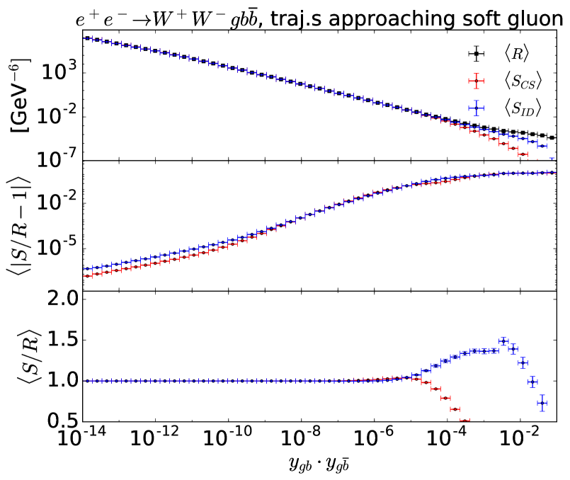
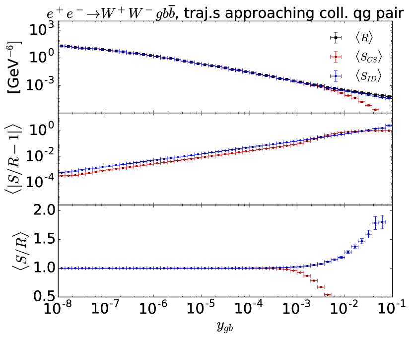
Figure 7: Matrix elements $R=\left|\mathcal{M}_{R}\right|^{2}$ and sum of associated dipoles $S=\sum\mathcal{D}$ (standard CS-dipoles in red, pseudo-dipoles in blue) for the process $e^{+}e^{-}\to W^{+}W^{-}gb\bar{b}$. Both dipole-types are evaluated on the same trajectory like described in the text.
Right: Average over trajectories in phase-space with increasingly soft gluon, left: Average over trajectories with increasingly collinear qg-pair.

We construct ensembles of phase-space points that we refer to as phase-space trajectories as follows: random phase-space points are sampled according to the real-emission cross section in the narrow-width approximation, while requesting three identified jets according to the Durham jet algorithm Catani:1991hj . For each phase-space point, the kinematical configuration is scaled according to the algorithm described in App. A in order to obtain a sequence of points that approach the soft or collinear limit.

Figure 7 shows the values of the real-emission matrix-element, $R=\left|\mathcal{M}_{R}\right|^{2}$ and the sum of the associated dipoles ($S=\sum\mathcal{D}$), as well as their ratio for the soft limit (left) and the $bg$–collinear limit (right) limit. We have averaged – for all sub-plots – over all entries within a bin. In doing so, the ratio plots enable us to assess the pointwise convergence of $S/R$ best. It can be seen that the cancellation of divergences occurs in both the standard CS subtraction method and in the pseudo-dipole approach, but that the pseudo-dipoles converge faster towards the real-emission matrix element, which can be seen in the lower panels of the figures.

3.1.2 $pp\to W^{+}W^{-}j_{b}j_{b}$

Next we consider the analogue to the above example at hadron colliders, namely the reaction $pp\to W^{+}W^{-}j_{b}j_{b}$, where $j_{b}$ indicates a $b$-tagged jet. To parametrize the soft and collinear trajectories in this process, we use the following variables

$$v_{i}^{0}=\frac{p_{i}p_{0}}{p_{0}p_{1}}\hskip 28.45274pt\mathrm{and}\hskip 28.45274ptv_{i}^{1}=\frac{p_{i}p_{1}}{p_{0}p_{1}}$$ (42)

where $p_{0}$ and $p_{1}$ are the momenta of the initial-state partons and $p_{i}$ is the momentum of the additional parton in the real correction. The phase-space trajectories are again constructed by generating random phase-space points with well separated partons, which are then modified according to the algorithm in App. A to obtain additional phase-space points that approach the singular limits.

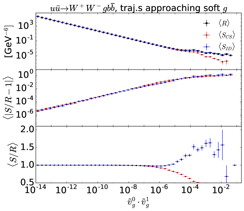
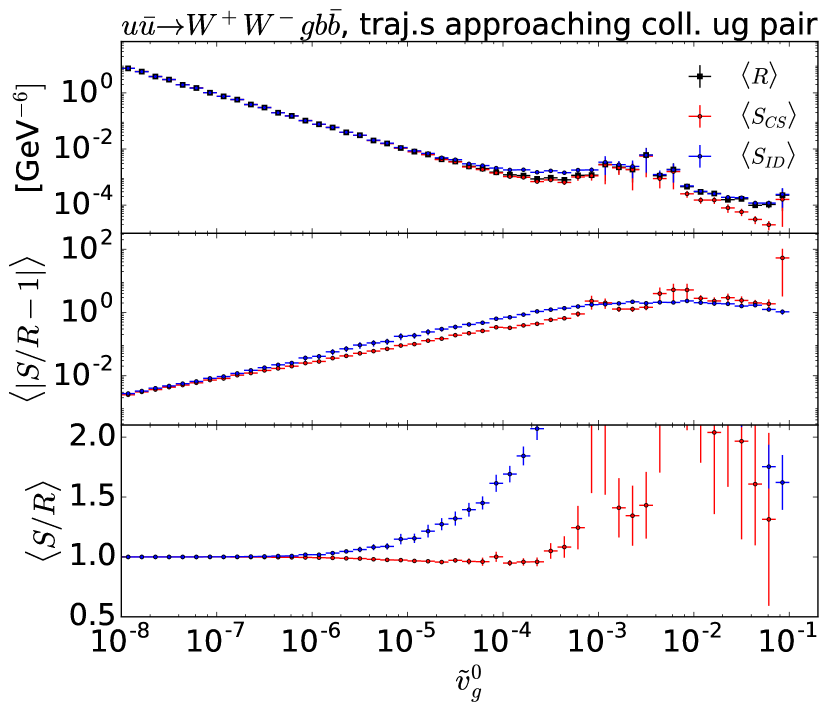
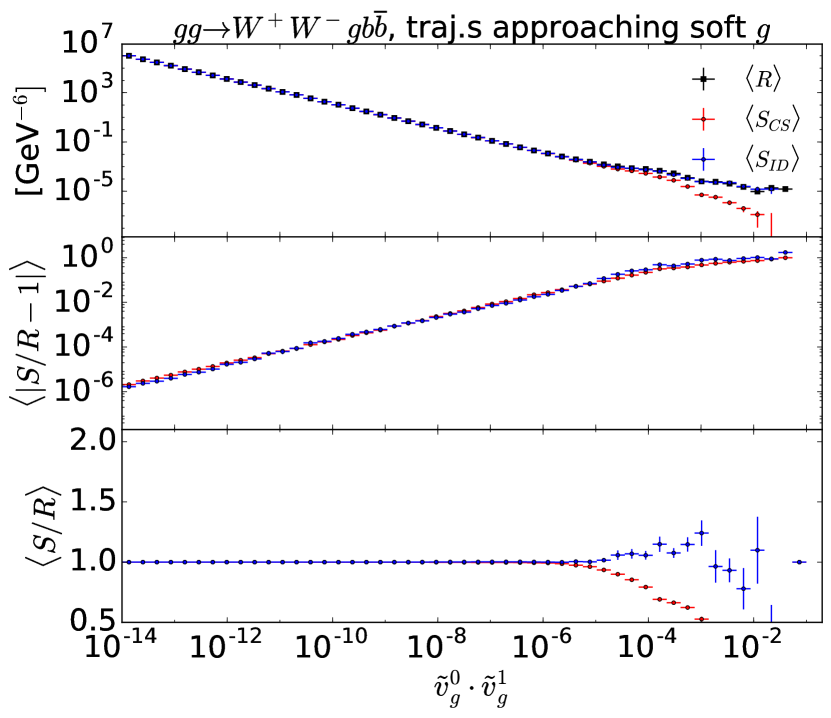
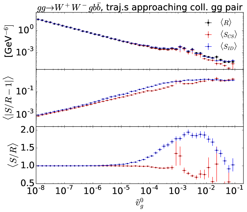
Figure 8: Matrix elements $R=\left|\mathcal{M}_{R}\right|^{2}$ and sum of associated dipoles $S=\sum\mathcal{D}$ (standard CS-dipoles in red, pseudo-dipoles in blue) for the processes $u\bar{u}\to W^{+}W^{-}gb\bar{b}$ (top) and $gg\to W^{+}W^{-}gb\bar{b}$ (bottom). Both dipole-types are evaluated on the same trajectories like described in the text.
Left: Average over trajectories in phase-space with increasingly soft gluon. Right: Average over trajectories with increasingly collinear partons.

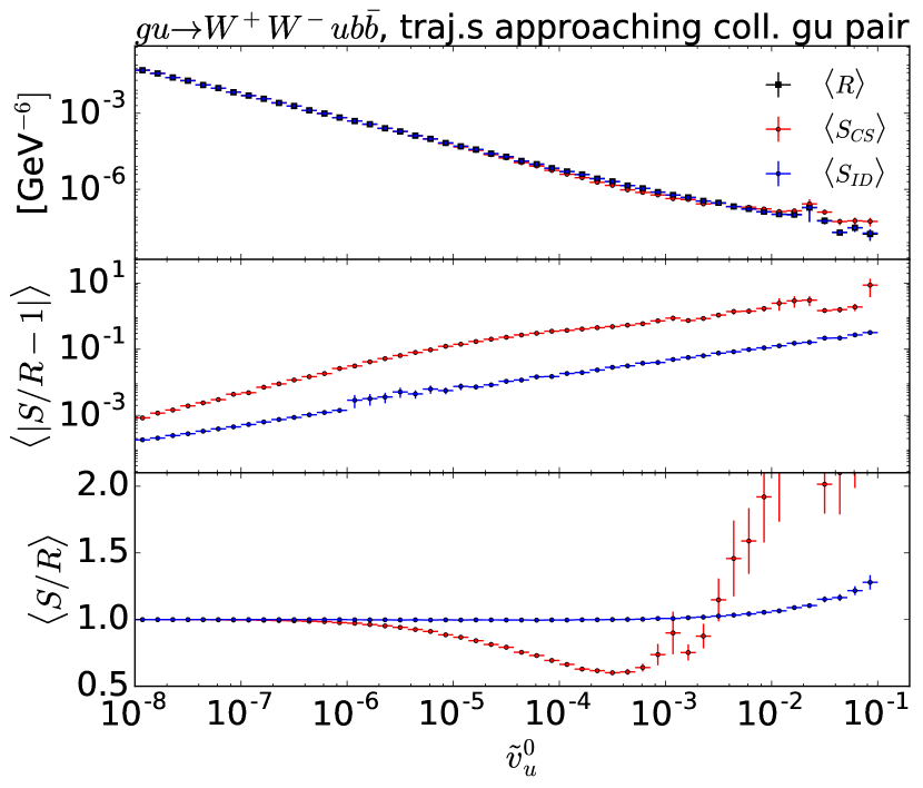
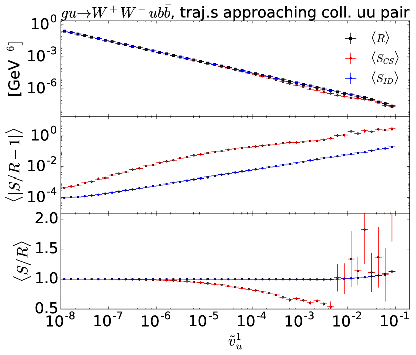
Figure 9: Matrix elements $R=\left|\mathcal{M}_{R}\right|^{2}$ and sum of associated dipoles $S=\sum\mathcal{D}$ (standard CS-dipoles in red, pseudo-dipoles in blue) for the process $ug\to W^{+}W^{-}ub\bar{b}$. Both dipole-types are evaluated on the same trajectories, with increasingly collinear partons, like described in the text.
Left: The $u$-quark in the final state becomes collinear to the first initial-state parton. Right: The $u$-quark in the final state becomes collinear to the second initial-state parton.

Figures 8 and 9 display the average values of the real-emission matrix element and the corresponding dipole subtraction terms, as well as their ratio – averaged within each bin – for processes with an additional gluon (Fig. 8) and an additional quark (Fig. 9) in the final state. The former develop both soft and collinear singularities, shown in the left and right panels of Fig. 8, respectively, while the latter only feature collinear singularities. Combining all tests, we validate all four initial-state splitting functions in Eq. (15).

It can be seen that both the standard CS- as well as the pseudo-dipoles converge towards the real correction. In the soft limit, which is the numerically more important one, the pseudo-dipoles converge faster. This is also the case for the collinear limit probed in Fig. 9. However, for the collinear limits tested on the right-hand side of Fig. 8 this is not the case. As a reason for this we suspect that the pseudo-dipole splitting functions Eq. (15) converge more slowly towards the associated Altarelli-Parisi functions than the standard CS ones.

3.2 Physical cross sections

In this section we present first results validating the pseudo-dipole subtraction method for resonance-aware processes at the level of observable cross sections and distributions. Results are cross-checked using two different implementations of our new algorithm within the public event generation framework Sherpa Gleisberg:2003xi ; Gleisberg:2008ta , one using the matrix-element generator AMEGIC++ Krauss:2001iv ; Gleisberg:2007md , and one using the new interface between Sherpa and OpenLoops Jones:2017giv . In this interface, the color-correlated Born matrix-elements are imported from OpenLoops libraries Cascioli:2011va , while the splitting function is calculated in Sherpa and the integration is performed using the techniques implemented in AMEGIC++ Krauss:2001iv .

3.2.1 $e^{+}e^{-}\to W^{+}W^{-}b\bar{b}$

Again we investigate first the reaction $e^{+}e^{-}\to W^{+}W^{-}b\bar{b}$. We vary the center-of-mass energy of the collider to obtain predictions below, at and above the top-quark pair production threshold, and we do not include the effects of initial-state radiation. We require two hard jets at $y=(5\textrm{ GeV}/E_{\rm cms})^{2}$ defined according to the Durham jet algorithm Catani:1991hj . The running of the strong coupling is evaluated at two loops, and the reference value is set to $\alpha_{s}(M_{Z}^{2})=0.118$, where $M_{Z}=91.1876~{}{\rm GeV}$.

	$\sqrt{s}=3m_{W}$		$\sqrt{s}=2m_{t}$		$\sqrt{s}=4m_{t}$
$\sigma\mathrm{[fb]}$	CS	ID	CS	ID	CS	ID
RS	$-0.00772(6)$	$-0.00140(5)$	$-0.52(3)$	$-2.85(1)$	$-9.5(4)$	$-5.3(1)$
BVI	$0.16143(13)$	$0.15506(13)$	$148.07(9)$	$150.55(9)$	$230.0(2)$	$226.0(2)$
$\sum$	$0.15371(14)$	$0.15366(14)$	$147.55(9)$	$147.70(9)$	$220.5(4)$	$220.7(2)$

Table 1: NLO cross sections for $e^{+}e^{-}\to W^{+}W^{-}b\bar{b}$ at $\mu_{R}=m_{t}$ and varying center-of-mass energy, computed using standard CS subtraction terms (CS) or pseudo-dipoles (ID). The subtracted real-emission contributions (RS) were calculated using $10^{7}$ phase-space points. The Born, virtual corrections and integrated subtraction terms (BVI) were calculated using $3\cdot 10^{6}$ phase-space-points.

Table 1 shows the total cross sections as well as the individual contributions from the subtracted real-emission terms (RS) as well as Born, virtual corrections and integrated subtraction terms (BVI). As expected, the RS and BVI contributions differ between the standard CS subtraction method and the pseudo-dipole approach, but their sum agrees within the statistical accuracy of the Monte-Carlo integration. The cross section is significantly enhanced at and above the production threshold for a top-quark pair. For those two center-of-mass energies, we expect the pseudo-dipoles to give a more physical interpretation of the subtraction term and thus a reduced variance during the integration. This is confirmed in Fig.10, which shows the evolution of the Monte-Carlo error during the integration. In the case of pseudo-dipole subtraction at or above threshold, the uncertainty is indeed substantially lower than for standard CS-dipoles. Below threshold the performance of pseudo-dipole subtraction is similar to the standard technique.

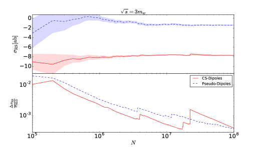
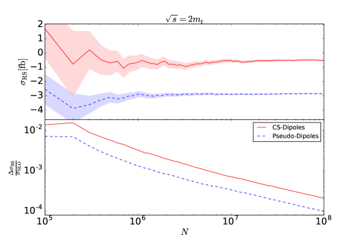
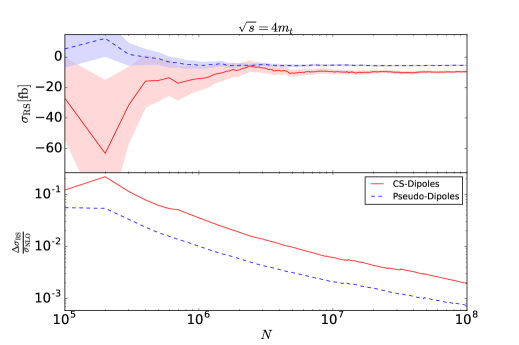
Figure 10: Evolution of the Monte-Carlo integration results for the subtracted real-emission contribution to the total cross section in $e^{+}e^{-}\to W^{+}W^{-}b\bar{b}$ at varying center-of-mass energy over number of sampled phase-space points $N$. From top to bottom: $\sqrt{s}=3m_{W}$, $\sqrt{s}=2m_{t}$ and $\sqrt{s}=4m_{t}$. Red solid lines show results from standard CS-dipoles, while blue dashed lines correspond to pseudo-dipoles. The colored bands in the upper panels and the lines in the lower panels show the one $\sigma$ statistical uncertainty of the Monte-Carlo integration.

Our validation is completed by a comparison of a few selected differential cross sections in the two subtraction schemes. Fig. 11 displays the invariant mass of the (anti-)top quark reconstructed at the level of the $W^{+}W^{-}b\bar{b}$ final state from the $W$-boson and a $b$-jet with a matching signed flavor tag. The deviation plot shows excellent statistical compatibility between the two simulations. It also displays clearly that the pseudo-dipole subtraction technique generates smaller statistical uncertainties than the standard CS subtraction method.

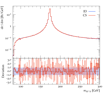
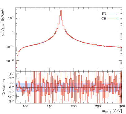
Figure 11: Invariant mass of the (anti-)top quark reconstructed at the level of the $W^{+}W^{-}b\bar{b}$ final state from the $W$-boson and a $b$-jet with a matching signed flavor tag.

3.2.2 $pp\to W^{+}W^{-}j_{b}j_{b}$

As a second application we consider the reaction $pp\to W^{+}W^{-}j_{b}j_{b}$, where $j_{b}$ indicates a $b$-tagged jet with $p_{T}>25$ GeV. We use the anti-$k_{T}$ jet algorithm Cacciari:2008gp with $R=0.4$. The total cross section and the individual contributions to the RS- and the BVI-cross-section for both standard CS- and pseudo-dipoles are given in Tab. 2. Again it can be seen that the convergence of the Monte-Carlo integration of the RS-cross-section for pseudo-dipoles is significantly better than the one for standard CS-dipoles. This can also be observed in Fig. 12, which is the analogue of Fig. 10 for the proton-proton initial state for a center-of-mass energy of $\sqrt{s}=13$ TeV.

	$\sqrt{s}=13$ TeV
$\sigma\mathrm{[pb]}$	CS	ID
RS	$-62.03(59)$	$-93.21(13)$
BVI	$360.02(39)$	$391.53(39)$
$\sum$	$297.99(71)$	$298.32(41)$

Table 2: NLO cross section for $pp\to W^{+}W^{-}j_{b}j_{b}$ at $\mu_{R}=\mu_{F}=m_{t}$ and $\sqrt{s}=13$ TeV, computed using standard CS subtraction terms (CS) or pseudo-dipoles (ID). The subtracted real-emission contributions (RS) were calculated using $10^{8}$ phase-space points. The Born, virtual corrections and integrated subtraction terms (BVI) were calculated using $8.5\cdot 10^{6}$ phase-space-points.

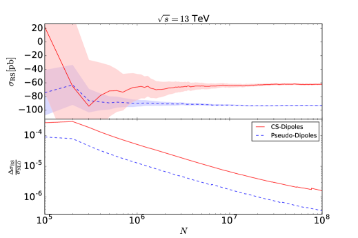
Figure 12: Evolution of the Monte-Carlo integration results for the subtracted real-emission contribution to the total cross section in $pp\to W^{+}W^{-}j_{b}j_{b}$ at $\sqrt{s}=13$ TeV over number of sampled phase-space points $N$. Red solid lines show results from standard CS-dipoles, while blue dashed lines correspond to pseudo-dipoles. The colored bands in the upper panels and the lines in the lower panels show the one $\sigma$ statistical uncertainty of the Monte-Carlo integration.

Finally, in Fig. 13 we confirm the agreement between standard CS-dipoles and pseudo-dipoles for the differential cross-sections as a function of the combined $W^{+}j_{b}$ and $W^{-}j_{\bar{b}}$ invariant mass. The two subtraction schemes agree within the statistical uncertainty and pseudo-dipoles exhibit a smaller statistical uncertainty.

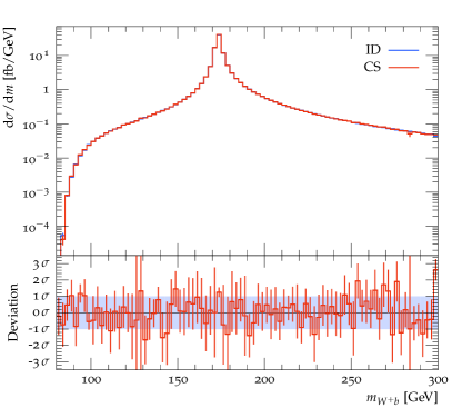
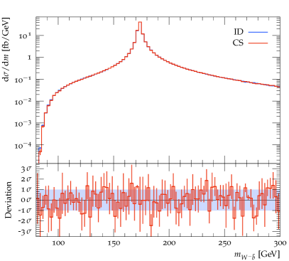
Figure 13: Invariant mass of the (anti-)top quark reconstructed at the level of the $W^{+}W^{-}j_{b}j_{b}$ final state from the $W$-boson and a $b$-jet with a matching flavor tag.

4 Conclusions

We have presented a technique that allows to preserve the virtuality of intermediate propagators in the computation of subtracted real-emission corrections to processes involving resonances. We have validated this approach in a simple fixed-order calculation and outlined how it can be generalized to more complicated processes. Due to the close correspondence with standard Catani-Seymour dipole subtraction, a matching to parton showers can be carried out in the MC@NLO or POWHEG methods in the future, thus paving the way for a precision measurement of processes involving for example single-top and top-quark pair production.

Appendix A Construction of phase-space trajectories

In this appendix we describe a generic method to generate phase-space trajectories approaching the soft or collinear limits of the hard matrix element, as used in Sec. 3.1. The technique is based on a suitable scaling of the Lorentz invariants parametrizing the desired limit. The corresponding kinematical configuration is determined by combining the appropriate final-state momenta using the massive dipole kinematics of Catani:2002hc and subsequently constructing a new real-emission configuration by applying the techniques in Hoeche:2009xc .

Initial state			Final state
$a\to\rm emit$, $b\to\rm spec$			$i\to g$, $j\to W$, $k\to b$
	soft	collinear		soft	collinear
$v_{i}^{\prime}$	$\lambda v_{i}$	$\lambda v_{i}$	$y^{\prime}$	$\lambda y$	$\displaystyle y\,\frac{1-\lambda\tilde{z}(1-y)}{1-\tilde{z}(1-y)}$
$x_{i,ab}^{\prime}$	$1-\lambda(1-x_{i,ab})$	$x_{i,ab}$	$\tilde{z}^{\prime}$	$\displaystyle\lambda\tilde{z}\frac{1-y}{1-\lambda y}$	$\displaystyle\lambda\tilde{z}(1-y)\left[1-y\,\frac{1-\lambda\tilde{z}(1-y)}{1-\tilde{z}(1-y)}\right]^{-1}$

Table 3: Scaling of Catani-Seymour parameters defined in Eqs. (43) and (44) used to construct the phase-space trajectories in Sec. 3.1. The scaling parameter is denoted by $\lambda$, and the gluon is labeled as particle $i$.

We use the notation and definitions of Catani:1996vz for final-state splittings with final-state spectator

$$\tilde{z}_{i}=\frac{p_{i}p_{k}}{(p_{i}+p_{j})p_{k}}\;,\qquad y_{ij,k}=\frac{p_{i}p_{j}}{p_{i}p_{j}+(p_{i}+p_{j})p_{k}}\;,$$ (43)

and for initial-state splitting with initial-state sepctator

$$x_{i,ab}=\frac{p_{a}p_{b}-p_{i}p_{a}-p_{i}p_{b}}{p_{a}p_{b}}\;,\qquad v_{i}=\frac{p_{i}p_{a}}{p_{a}p_{b}}\;.$$ (44)

Table 3 gives the assignment of the momenta to the labels $i$, $j$ and $k$ / $a$, $b$ and $i$ for the pseudo-dipoles and shows how $y$ and $\tilde{z}$ / $v$ and $x$ are rescaled in order to construct the phase-space trajectories.

The construction of momenta in the final-state splitter case proceeds as follows: We first combine the three momenta $p_{i}$, $p_{j}$ and $p_{k}$ into intermediate momenta $\tilde{p}_{k}$ and $\tilde{p}_{ij}=q-\tilde{p_{k}}$, where $q=p_{i}+p_{j}+p_{k}$.

$$\begin{split}\tilde{p}_{k}^{\,\mu}=&\;\left(p_{k}^{\,\mu}-\frac{q\cdot p_{k}}{q^{2}}\,q^{\mu}\right)\,\sqrt{\frac{\lambda(q^{2},m_{ij}^{2},m_{k}^{2})}{\lambda(q^{2},s_{ij},m_{k}^{2})}}+\frac{q^{2}+m_{k}^{2}-m_{ij}^{2}}{2\,q^{2}}\,q^{\mu}\;,\end{split}$$ (45)

where the Källen function is given by $\lambda(a,b,c)=(a-b-c)^{2}-4\,bc$. Using the scaled parameters $y$ and $\tilde{z}$ from Tab. 3 we compute the new mass of the pseudoparticle $ij$ as $s_{ij}=y\,(q^{2}-m_{k}^{2})+(1-y)\,(m_{i}^{2}+m_{j}^{2})$, and use Eq. (45) with $\tilde{p}_{k}\leftrightarrow p_{k}$ and $m_{ij}\leftrightarrow s_{ij}$ to recalculate $p_{k}$ and $p_{ij}$. The new momentum $p_{i}$ is then constructed as

$$p_{i}^{\mu}\,= \;\bar{z}\,\frac{\gamma(q^{2},s_{ij},m_{k}^{2})\,p_{ij}^{\mu}-s_{ij}\,p_{k}^{\mu}}{\beta(q^{2},s_{ij},m_{k}^{2})}+\frac{m_{i}^{2}+{\rm k}_{\perp}^{2}}{\bar{z}}\,\frac{p_{k}^{\mu}-m_{k}^{2}/\gamma(q^{2},s_{ij},m_{k}^{2})\,p_{ij}^{\mu}}{\beta(q^{2},s_{ij},m_{k}^{2})}+k_{\perp}^{\mu}\;,$$ (46)

where $\beta(a,b,c)={\rm sgn}(a-b-c)\sqrt{\lambda(a,b,c)}$ and $2\,\gamma(a,b,c)=(a-b-c)+\beta(a,b,c)$. The parameters $\bar{z}$ and ${\rm k}_{\perp}^{2}=-k_{\perp}^{2}$ of this decomposition are given by

$$\begin{split}\bar{z}\,=&\;\frac{q^{2}-s_{ij}-m_{k}^{2}}{\beta(q^{2},s_{ij},m_{k}^{2})}\,\left[\;\tilde{z}\,-\,\frac{m_{k}^{2}}{\gamma(q^{2},s_{ij},m_{k}^{2})}\frac{s_{ij}+m_{i}^{2}-m_{j}^{2}}{q^{2}-s_{ij}-m_{k}^{2}}\right]\;,\\ {\rm k}_{\perp}^{2}\,=&\;\bar{z}\,(1-\bar{z})\,s_{ij}-(1-\bar{z})\,m_{i}^{2}-\bar{z}\,m_{j}^{2}\;,\end{split}$$ (47)

The transverse momentum is constructed using an azimuthal angle, $\phi_{i}$

$$k_{\perp}^{\mu}={\rm k}_{\perp}\left(\cos\phi_{i}\frac{n_{\perp}^{\mu}}{|n_{\perp}|}+\sin\phi_{i}\frac{l_{\perp}^{\,\mu}}{|l_{\perp}|}\right)\;,$$ (48)

where

$$n_{\perp}^{\mu}=\epsilon^{0\mu}_{\;\;\;\nu\rho}\,\tilde{p}_{ij}^{\,\nu}\,\tilde{p}_{k}^{\,\rho}\;,\qquad l_{\perp}^{\,\mu}=\epsilon^{\mu}_{\;\nu\rho\sigma}\,\tilde{p}_{ij}^{\,\nu}\,\tilde{p}_{k}^{\,\rho}\,n_{\perp}^{\sigma}\;.$$ (49)

In kinematical configurations where $\vec{\tilde{p}}_{ij}=\pm\vec{\tilde{p}}_{k}$, $n_{\perp}$ defined as in Eq. (48) vanishes. It can then be computed as $n_{\perp}^{\mu}=\epsilon^{0\,i\mu}_{\;\;\;\;\;\nu}\,\tilde{p}_{ij}^{\,\nu}$, where $i$ may be any index that yields a nonzero result.

In the case of initial-state splitters, the construction proceeds as follows: We first combine the two momenta $p_{a}$ and $p_{i}$ into the intermediate momentum $\tilde{p}_{ai}$.

$$\begin{split}\tilde{p}_{ai}^{\,\mu}=&\;\left(p_{a}^{\,\mu}-\frac{m_{a}^{2}}{\gamma(s_{ab},m_{a}^{2},m_{b}^{2})}\,p_{b}^{\,\mu}\right)\,\sqrt{\frac{\lambda(q^{2},\tilde{m}_{ai}^{2},m_{b}^{2})}{\lambda(s_{ab},m_{a}^{2},m_{b}^{2})}}+\frac{\tilde{m}_{aij}^{2}}{\gamma(q^{2},\tilde{m}_{aij}^{2},m_{b}^{2})}\,p_{b}^{\,\mu}\;,\end{split}$$ (50)

where $q=p_{a}+p_{b}-p_{i}$ and $s_{ab}=(p_{a}+p_{b})^{2}$. We then apply a Lorentz transformation to all final-state momenta as $\tilde{p}^{\mu}=\Lambda^{\mu}_{\;\nu}p^{\nu}$, where

$$\Lambda(\tilde{q},q)^{\mu}_{\;\nu}=g^{\mu}_{\;\nu}-\frac{2\,(q+\tilde{q})^{\mu}(q+\tilde{q})_{\nu}}{(q+\tilde{q})^{2}}+\frac{2\,\tilde{q}^{\mu}q_{\nu}}{q^{2}}\;,$$ (51)

Using the scaled parameters $v$ and $x$ from Tab. 3 we compute the new invariant mass squared of the initial state as $s_{ab}=(q^{2}-m_{i})^{2}/x_{i,ab}-(m_{a}^{2}+m_{b}^{2})(1-x_{i,ab})/x_{i,ab}$ and use the inverse transformation of Eq. (50) to construct the initial-state momentum $p_{a}$. The new momentum $p_{i}$ is then defined as

$$\begin{split}p_{i}^{\,\mu}\,=&\;(1-\bar{z}_{ai})\,\frac{\gamma(s_{ab},m_{a}^{2},m_{b}^{2})\,p_{a}^{\,\mu}-m_{a}^{2}\,p_{b}^{\,\mu}}{\beta(s_{ab},m_{a}^{2},m_{b}^{2})}\\ &\;+\frac{m_{i}^{2}+{\rm k}_{\perp}^{2}}{1-\bar{z}_{ai}}\,\frac{p_{b}^{\,\mu}-m_{b}^{2}/\gamma(s_{ab},m_{a}^{2},m_{b}^{2})\,p_{a}^{\,\mu}}{\beta(s_{ab},m_{a}^{2},m_{b}^{2})}-k_{\perp}^{\mu}\;,\end{split}$$ (52)

with the transverse components constructed according to Eq. (48). The parameters $\bar{z}_{aij}$ and ${\rm k}_{\perp}^{2}=-k_{\perp}^{2}$ of this decomposition are given by

$$\begin{split}\bar{z}_{ai}\,=&\;\frac{s_{ab}-m_{a}^{2}-m_{b}^{2}}{\beta(s_{ab},m_{a}^{2},m_{b}^{2})}\,\left[\;x_{i,ab}+v_{i}\,-\,\frac{m_{b}^{2}}{\gamma(s_{ab},m_{a}^{2},m_{b}^{2})}\frac{s_{ai}+m_{a}^{2}-m_{i}^{2}}{s_{ab}-m_{a}^{2}-m_{b}^{2}}\right]\;,\\ {\rm k}_{\perp}^{2}\,=&\;\bar{z}_{ai}\,(1-\bar{z}_{ai})\,m_{a}^{2}-(1-\bar{z}_{ai})\,s_{ai}-\bar{z}_{ai}\,m_{i}^{2}\;,\end{split}$$ (53)

Finally we boost all remaining final-state particles according to Eq. (51) with $q\leftrightarrow\tilde{q}$.

References

• (1) K. Agashe et al., Working Group Report: Top Quark, in Proceedings, 2013 Community Summer Study on the Future of U.S. Particle Physics: Snowmass on the Mississippi (CSS2013): Minneapolis, MN, USA, July 29-August 6, 2013, 2013. 1311.2028.
• (2) P. Nason, S. Dawson and R. K. Ellis, The One Particle Inclusive Differential Cross-Section for Heavy Quark Production in Hadronic Collisions, Nucl. Phys. B327 (1989) 49–92.
• (3) W. Beenakker, W. L. van Neerven, R. Meng, G. A. Schuler and J. Smith, QCD corrections to heavy quark production in hadron hadron collisions, Nucl. Phys. B351 (1991) 507–560.
• (4) M. L. Mangano, P. Nason and G. Ridolfi, Heavy quark correlations in hadron collisions at next-to-leading order, Nucl. Phys. B373 (1992) 295–345.
• (5) S. Frixione, M. L. Mangano, P. Nason and G. Ridolfi, Top quark distributions in hadronic collisions, Phys. Lett. B351 (1995) 555–561, [hep-ph/9503213].
• (6) P. Bärnreuther, M. Czakon and A. Mitov, Percent Level Precision Physics at the Tevatron: First Genuine NNLO QCD Corrections to $q\bar{q}\to t\bar{t}+X$, Phys. Rev. Lett. 109 (2012) 132001, [1204.5201].
• (7) M. Czakon and A. Mitov, NNLO corrections to top pair production at hadron colliders: the quark-gluon reaction, JHEP 01 (2013) 080, [1210.6832].
• (8) M. Czakon, P. Fiedler and A. Mitov, Total Top-Quark Pair-Production Cross Section at Hadron Colliders Through $O(\alpha_{s}^{4})$, Phys. Rev. Lett. 110 (2013) 252004, [1303.6254].
• (9) M. Czakon, D. Heymes, A. Mitov, D. Pagani, I. Tsinikos and M. Zaro, Top-pair production at the LHC through NNLO QCD and NLO EW, JHEP 10 (2017) 186, [1705.04105].
• (10) D. Gonçalves-Netto, D. López-Val, K. Mawatari, T. Plehn and I. Wigmore, Automated Squark and Gluino Production to Next-to-Leading Order, Phys. Rev. D87 (2013) 014002, [1211.0286].
• (11) A. Denner, S. Dittmaier, S. Kallweit and S. Pozzorini, NLO QCD corrections to WWbb production at hadron colliders, Phys. Rev. Lett. 106 (2011) 052001, [1012.3975].
• (12) G. Bevilacqua, M. Czakon, A. van Hameren, C. G. Papadopoulos and M. Worek, Complete off-shell effects in top quark pair hadroproduction with leptonic decay at next-to-leading order, JHEP 02 (2011) 083, [1012.4230].
• (13) A. Denner, S. Dittmaier, S. Kallweit and S. Pozzorini, NLO QCD corrections to off-shell top-antitop production with leptonic decays at hadron colliders, JHEP 10 (2012) 110, [1207.5018].
• (14) G. Heinrich, A. Maier, R. Nisius, J. Schlenk and J. Winter, NLO QCD corrections to $W^{+}W^{-}b\bar{b}$ production with leptonic decays in the light of top quark mass and asymmetry measurements, JHEP 06 (2014) 158, [1312.6659].
• (15) S. Frixione and B. R. Webber, Matching NLO QCD computations and parton shower simulations, JHEP 06 (2002) 029, [hep-ph/0204244].
• (16) S. Frixione, P. Nason and G. Ridolfi, A Positive-weight next-to-leading-order Monte Carlo for heavy flavour hadroproduction, JHEP 09 (2007) 126, [0707.3088].
• (17) T. Ježo and P. Nason, On the Treatment of Resonances in Next-to-Leading Order Calculations Matched to a Parton Shower, JHEP 12 (2015) 065, [1509.09071].
• (18) T. Ježo, J. M. Lindert, P. Nason, C. Oleari and S. Pozzorini, An NLO+PS generator for $t\bar{t}$ and $Wt$ production and decay including non-resonant and interference effects, Eur. Phys. J. C76 (2016) 691, [1607.04538].
• (19) R. Frederix, S. Frixione, A. S. Papanastasiou, S. Prestel and P. Torrielli, Off-shell single-top production at NLO matched to parton showers, JHEP 06 (2016) 027, [1603.01178].
• (20) S. Ferrario Ravasio, T. Ježo, P. Nason and C. Oleari, A theoretical study of top-mass measurements at the LHC using NLO+PS generators of increasing accuracy, Eur. Phys. J. C78 (2018) 458, [1801.03944].
• (21) T. Ježo, J. M. Lindert, N. Moretti and S. Pozzorini, New NLOPS predictions for $\boldsymbol{t\bar{t}+b}$ -jet production at the LHC, Eur. Phys. J. C78 (2018) 502, [1802.00426].
• (22) S. Frixione, Z. Kunszt and A. Signer, Three jet cross-sections to next-to-leading order, Nucl. Phys. B467 (1996) 399–442, [hep-ph/9512328].
• (23) S. Catani and M. H. Seymour, A General algorithm for calculating jet cross-sections in NLO QCD, Nucl. Phys. B485 (1997) 291–419, [hep-ph/9605323].
• (24) S. Catani, S. Dittmaier, M. H. Seymour and Z. Trocsanyi, The Dipole formalism for next-to-leading order QCD calculations with massive partons, Nucl. Phys. B627 (2002) 189–265, [hep-ph/0201036].
• (25) K. Fujii et al., Physics Case for the International Linear Collider, 1506.05992.
• (26) A. Arbey et al., Physics at the e+ e- Linear Collider, Eur. Phys. J. C75 (2015) 371, [1504.01726].
• (27) ATLAS collaboration, M. Aaboud et al., Probing the quantum interference between singly and doubly resonant top-quark production in $pp$ collisions at $\sqrt{s}=13$ TeV with the ATLAS detector, Submitted to: Phys. Rev. Lett. (2018) , [1806.04667].
• (28) T. Gleisberg and F. Krauss, Automating dipole subtraction for QCD NLO calculations, Eur. Phys. J. C53 (2008) 501–523, [0709.2881].
• (29) S. Catani, Y. L. Dokshitzer, M. Olsson, G. Turnock and B. R. Webber, New clustering algorithm for multijet cross sections in $e^{+}e^{-}$ annihilation, Phys. Lett. B269 (1991) 432–438.
• (30) T. Gleisberg, S. Höche, F. Krauss, A. Schälicke, S. Schumann and J. Winter, Sherpa 1.$\alpha$, a proof-of-concept version, JHEP 02 (2004) 056, [hep-ph/0311263].
• (31) T. Gleisberg, S. Höche, F. Krauss, M. Schönherr, S. Schumann, F. Siegert et al., Event generation with Sherpa 1.1, JHEP 02 (2009) 007, [0811.4622].
• (32) F. Krauss, R. Kuhn and G. Soff, AMEGIC++ 1.0: A Matrix Element Generator In C++, JHEP 02 (2002) 044, [hep-ph/0109036].
• (33) S. Jones and S. Kuttimalai, Parton Shower and NLO-Matching uncertainties in Higgs Boson Pair Production, JHEP 02 (2018) 176, [1711.03319].
• (34) F. Cascioli, P. Maierhofer and S. Pozzorini, Scattering Amplitudes with Open Loops, Phys. Rev. Lett. 108 (2012) 111601, [1111.5206].
• (35) M. Cacciari, G. P. Salam and G. Soyez, The anti-$k_{t}$ jet clustering algorithm, JHEP 04 (2008) 063, [0802.1189].
• (36) S. Höche, S. Schumann and F. Siegert, Hard photon production and matrix-element parton-shower merging, Phys. Rev. D81 (2010) 034026, [0912.3501].