Enhancement of chemotherapy using oncolytic virotherapy: Mathematical and optimal control analysis
Abstract.
Oncolytic virotherapy has been emerging as a promising novel cancer treatment which may be further combined with the existing therapeutic modalities to enhance their effects. To investigate how virotherapy could enhance chemotherapy, we propose an ODE based mathematical model describing the interactions between tumour cells, the immune response, and a treatment combination with chemotherapy and oncolytic viruses. Stability analysis of the model with constant chemotherapy treatment rates shows that without any form of treatment, a tumour would grow to its maximum size. It also demonstrates that chemotherapy alone is capable of clearing tumour cells provided that the drug efficacy is greater than the intrinsic tumour growth rate. Furthermore, virotherapy alone may not be able to clear tumour cells from body tissue but would rather enhance chemotherapy if viruses with high viral potency are used. To assess the combined effect of virotherapy and chemotherapy we use the forward sensitivity index to perform a sensitivity analysis, with respect to chemotherapy key parameters, of the virus basic reproductive number and the tumour endemic equilibrium. The results from this sensitivity analysis indicate the existence of a critical dose of chemotherapy above which no further significant reduction in the tumour population can be observed. Numerical simulations show that a successful combinational therapy of the chemotherapeutic drugs and viruses depends mostly on the virus burst size, infection rate, and the amount of drugs supplied. Optimal control analysis was performed, by means of the Pontryagin’s maximum principle, to further refine predictions of the model with constant treatment rates by accounting for the treatment costs and sides effects. Results from this analysis suggest that the optimal drug and virus combination correspond to half their maximum tolerated doses. This is in agreement with the results from stability and sensitivity analyses.
Key words and phrases:
Chemovirotherapy, Oncolytic virotherapy, optimal drug, virus combination.1991 Mathematics Subject Classification:
Primary: 49K15; Secondary: 92B05.Joseph Malinzi∗1, Rachid Ouifki1
1 Department of Mathematics and Applied Mathematics, University of Pretoria,
Private Bag X 20, Hatfield, Pretoria 0028, South Africa
Amina Eladdadi∗2, Delfim F.M. Torres3 and K.A. Jane White4
2Department of Mathematics, The College of Saint Rose, Albany, New York, USA
3Center for Research and Development in Mathematics and Applications (CIDMA),
Department of Mathematics, University of Aveiro, 3810-193 Aveiro, Portugal
4Department of Mathematical Sciences, University of Bath,
Claverton Down, Bath BA2 7AY, UK
1. Introduction
Combination therapy strategies have shown significant promise for treating cancers that are resistant to conventional modalities. Oncolytic virotherapy (OV) is an emerging treatment modality that uses replication competent viruses to destroy cancers [22, 43, 27, 30]. Their tumour specific properties allow for viral binding, entry, and replication [32]. Various studies have investigated combination strategies with OV and chemotherapeutic drugs to optimize both viral oncolysis and the effect of the added therapy [8, 32, 41]. Oncolytic viruses can greatly enhance the cytotoxic mechanisms of chemotherapeutics [35]. Furthermore, chemotherapeutic drugs lyse fast multiplying cells and, in general, virus infected tumour cells quickly replicate [5]. In most combination studies with chemotherapy drugs, apoptosis was increased but viral replication was not enhanced [32, 49, 3]. For example, Nguyen et al. [32] gave an account of the mechanisms through which drugs can successfully be used in a combination with oncolytic viruses. They, however, noted that the success of this combination depended on several factors including the type of oncolytic virus (OV)-drug combination used, the timing, frequency, dosage, and cancer type targeted. A review of recent clinical studies by Binz and Urlrich [8] shows the classification of possible combination of drugs and oncolytic viruses. Oncolytic virotherapy is still ongoing clinical trials [49, 3], and some virus-drug combos, for example talimogene laherparepvec, have been approved for the treatment of melanoma [51].
While, there is a growing body of scientific research showing that combination therapies are the cutting edge for cancer treatment, the design of an optimal protocol remains an open question. The chemo-viro therapy combination is no exception. Despite a noticeable success in the clinical and experimental studies to investigate and characterise the treatment of cancer with chemotherapeutics-virus combinations, much is still not understood about chemovirotherapy. Some of the main open questions in designing an optimal chemovirotherapy treatment are figuring out the right dose combination, the most effective method of drug infusion, and the important treatment characteristics [25].
Mathematical modelling and optimal control theory have over the years played an important role in answering such important research questions which would cost much to set up experimentally. Several mathematical studies including [15, 28, 37] have addressed the dynamics of oncolytic virotherapy treatment. For example, Ursher [50] gave a summary of some mathematical models for chemotherapy. Tian [47] presented a mathematical model that incorporates burst size for oncolytic virotherapy. His analysis showed that there are two threshold burst size values and below one of them the tumour always grows to its maximum size. His study affirmed that a tumour can be greatly reduced to low undetectable cell counts when the burst size is large enough. A recent study by Malinzi et al. [29] showed that that chemotherapy alone was not able to deplete tumour cells from body tissue but rather in unison with oncolytic viruses could possibly reduce the tumour concentration to a very low undetectable state. Other similar mathematical models on virotherapy include [30, 53, 54, 33, 1].
In this paper, we address the question on: “what is the optimal chemotherapeutic drug and virus dosage combination for the elimination of tumour cells in body tissue?” To this end, we develop a mathematical model and optimal control problem that account for the combination of cancer treatment using chemotherapy and virotherapy. The paper is organised as follows. Section 2 is devoted to the model description and the underlying assumptions. In Section 3, we analyse three sub-models: without-treatment model, chemotherapy-only model, and the oncolytic virotherapy-only model. The analysis of the whole model, that is, the chemotherapeutic drug combined with the virus therapy is detailed in Section 4. In Section 5, we investigate an optimal control problem with a quadratic objective function to determine the optimal dosage combination of the chemotherapy drug and the virotherapy. The numerical simulations illustrating our theoretical results are presented in Section 6. We conclude with a discussion in Section 7.
2. Model Formulation
In this section, we propose and formulate our new mathematical model describing the growth of an avascular solid tumour under the effect of both chemotherapy and oncolytic virotherapy treatments. The model considers six state variables summarized in Table 1. We first start by stating the underlying model assumptions in Subsection 2.1, followed by the model equations and their detailed description in Subsection 2.2.
2.1. Model description and assumptions
To model the effects of the chemo-virotherapy on the tumour, we consider the dynamics of the following interacting cell populations: tumour cells (both uninfected and virus-infected cells), immune cells (both virus and tumour specific immune responses), the free virus and the drug concentrations. Based on the discussion above and the scientific literature on the interactions between the uninfected and the virus-infected tumour cells in the presence of the oncolytic virotherapy and chemotherapy treatments, the following assumptions are made in setting up the model:
-
(1)
Without treatment, the tumour grows logistically with a carrying capacity [47].
- (2)
-
(3)
The model accounts for both virus and tumour specific immune responses [21].
-
(4)
Virus production is a function of virus burst size and the death of infected immune cells. The number of viruses therefore increases as infected tumour cells density multiplies [47].
-
(5)
We consider both virus and tumour specific immune responses. Virus-specific immune response is proportional to the infected tumour cell numbers whilst the tumour specific immune response is taken to be of Michaelis–Menten form to account for saturation in the immune proliferation [23].
-
(6)
We consider a case where drug infusion per day is constant. The constant infusion rate may relate to a situation where a patient is put on an intravenous injection or a protracted venous infusion and the drug is constantly pumped into the body. This form of drug dissemination is used on cancer patients who stay in the hospital for a long period of time. Higher doses of certain anti-cancer drugs may however lead to hepatic veno-occlusive disease, a condition where the liver is obstructed as a result of using high-dose chemotherapy [12, 55]. Another more realistic consideration would be to use periodic infusion [7, 48]. This would lead to a periodic system of equations for which standard theory on periodic systems applies (see for example [36]). This case is, however, not dealt with in this work, and will be studied in a future work.
2.2. Model equations
The proposed mathematical model consists of the following system of six differential equations (1)–(6):
| (1) | ||||
| (2) | ||||
| (3) | ||||
| (4) | ||||
| (5) | ||||
| (6) |
The model variables and parameters, their meaning and base values are summarised in Table 1 and Table 2 respectively.
| Variable | Description | Units |
|---|---|---|
| Uninfected tumour density | cells per mm3 | |
| Virus infected tumour cell density | cells per mm3 | |
| Free virus particles | virions per mm3 | |
| Virus specific immune response | cells per mm3 | |
| Tumour specific immune response | cells per mm3 | |
| Drug concentration | grams per millilitre (g/ml) |
The initial conditions for the model are:
| (7) |
where the constants , , , , , and denote the initial concentrations of the uninfected tumour, virus infected tumour, free virus particles, virus specific immune, tumour specific immune, and the chemotherapeutic drug respectively. They are assumed to be nonnegative to make sense biologically. A detailed description of the model follows.
In Eqs. (1) & (2), the terms represents tumour growth. The term describes infection of tumour cells by the virus where is the infection rate. Drug effect to the uninfected and infected tumour cells is respectively described by the terms and where and are lysis induced rates. and are Michaelis–Menten constants and relate to killing rates when the virus and the drug are half-maximal [42, 2, 39]. The term represents tumour specific immune response where is the uninfected lysis rate by tumour specific immune cells. Infected tumour cells have a lifespan and are killed by both tumour and virus specific immune cells. These are described by the terms and where is the natural death rate, and are respectively lysis rates of tumour cells by the tumour specific and virus specific immune cells.
In Eq. (3), the term represents virus proliferation where is the virus burst size and is the infected tumour cell death rate. The term represents loss of free virus due to infection of the uninfected tumour cells. Virus deactivation in body tissue is represented by the term where is the rate of decay.
In Eqs. (4) & (5), is the virus specific immune production and represents its deactivation where is the decay rate. The term represents tumour-specific immune response where is the rate of production and is a Michaelis constant. Tumour-specific immune decay is described by the term where is the rate of decay.
In Eq. (6), the time dependent function represents drug infusion into the tumour and describes drug decay where is the rate of decay.
| Symbol | Description | Value & units | Ref. |
|---|---|---|---|
| Tumour carrying capacity | cells per mm3 per day | [4] | |
| Tumour growth rate | cells per mm3 per day | [4] | |
| Infection rate of tumour cells | cells per mm3 per day | [4] | |
| Infected tumour cells death | day-1 | [4] | |
| Rate of virus decay | day-1 | [4] | |
| Virus burst size | virions per mm3 per day | [11] | |
| Rate drug decay | millilitres per mm3 per day | [38] | |
| Lysis rate of by the drug | cells per mm3 per day | [38] | |
| Lysis rate of by the drug | cells per mm3 per day | [38] | |
| production rate | day-1 | [9] | |
| production rate | cells per mm3 per day | [18, 26] | |
| immune decay rates | day-1 | [18, 26] | |
| Michaelis–Menten constants | cells per mm3 per day | [24] | |
| Lysis rate of by | cells per mm3 per day | est | |
| Lysis rate of by | cells per mm3 per day | est | |
| Lysis rate of by | cells per mm3 per day | est |
3. Mathematical analysis
To better understand the dynamics of the proposed model, we begin by examining the model’s behaviour about the steady states. This analysis is crucial for identifying the conditions necessary to achieve a tumour-free state. We first show that the model is well posed in a biologically feasible domain, and then proceed with a stability analysis of the model with constant drug infusion. We then analyse the model in the case of no treatment, with chemotherapy alone, and with oncolytic virotherapy alone. The case of the chemotherapeutic drug combined with the virus therapy is detailed as well.
3.1. Well-posedness
Before we proceed with the mathematical analysis, we need to show that the model is well posed in a biologically feasible domain. The model describes the temporal evolution of cell populations, therefore, the cell densities should remain non negative and bounded. The well-posedness theorem is stated below and the proofs are given in Appendix A.
Theorem 3.1.
- (i)
-
(ii)
If , , , and , then , , , , and for all .
-
(iii)
The trajectories evolve in an attracting region , where is the maximum drug concentration and depends on the infusion method.
- (iv)
We will analyse the model quantitative behaviour in the domain .
3.2. Without-treatment model
To investigate the efficacy of each treatment, their combination as well as the immune response to tumour cells, we first study the model without any form of treatments. The model system of eqs. (1)–( 6) without treatment reduces to the following system describing the interactions of the uninfected tumour with the tumour specific immune cells:
| (8) |
Proposition 1.
The model (3.2) has two biologically meaningful steady states: a tumour-free state, , which is unstable and a tumour endemic state,
| (9) |
where , which is locally asymptotically stable.
Proof.
Equating Eqs. (3.2) to zero yields:
| (10) | ||||
| (11) |
From which if then . The eigenvalues of the Jacobian matrix of the model (3.2) evaluated at are and . One positive and the other negative. Implying that the tumour free equilibrium is unstable. Compare Equation (10) to . We observe that implying that and therefore there is only one positive root of the quadratic equation (10) and its given by
The characteristic polynomial of the Jacobian matrix evaluated at is given by
| (12) |
We prove in Appendix B, using Routh–Hurwitz criterion, that and and thus the endemic steady state, , is locally asymptotically stable. ∎
Biological interpretation: Proposition 1 suggests that, without any form of treatment, the tumour-free state is always unstable and the endemic state is stable implying that the tumour would not be eliminated from the body.
3.3. Chemotherapy-only model
We consider a case where drug infusion per day is constant, that is, . The model with chemo-only, that is , reduces to:
| (13) |
Proposition 2.
Proof.
Setting Equations in (3.3) to zero gives:
| (15) | ||||
| (16) |
from which if then . The eigenvalues of the Jacobian of (3.3) evaluated at are , and implying that for to be negative, then . If then from Equation (15),
which when solved, and using the same analysis as in Proposition 1, gives the expressions in Equation (2). The characteristic polynomial of the Jacobian matrix evaluated at is given in Equation (32). It directly follows from Routh–Hurwitz criterion that the tumour endemic state, , is locally asymptotically stable if the conditions (B) are fulfilled. ∎
Biological interpretation:
Proposition 2 suggests that a tumour can be eradicated
by chemotherapy from the body tissue if the tumour growth rate
is less than the drug efficacy (). Otherwise,
it would continue to grow uncontrollably.
Since drug dosage, , must not exceed the Maximum Tolerable Dose (MTD),
denoted by , we further derive the following result in Proposition 3:
Proposition 3.
-
(1)
If , the tumour-free state will always be unstable for any .
-
(2)
If :
-
(i)
If , then the tumour-free state is unstable for all .
-
(ii)
If , then the tumour-free state is locally asymptotically stable for all .
-
(i)
Proof.
-
(1)
From the condition for stability in Proposition 2, if then , which violates the condition for stability.
-
(2)
If :
-
(i)
If , yet the drug dosage, , can not be larger than the MTD, , implying that the condition for stability in Proposition 2 is still violated.
-
(ii)
If , and then the stability condition if fulfilled.
-
(i)
∎
Biological interpretation: Proposition 3 suggests the followings:
-
(1)
For a chemotherapeutic drug that is not highly efficient () the tumour cannot be eradicated.
-
(2)
If the efficacy, , which is also the lysis rate measured in number of uninfected tumour cells lysed per mm3 per day, is high enough but with:
-
(i)
a very toxic drug, then one cannot give enough dose to eradicate the tumour
-
(ii)
a drug which is less toxic, then one can afford to give a dose which is not larger than the MTD and yet which allows for the condition for stability.
-
(i)
3.4. Virotherapy-only model
To determine the effect of virotherapy on tumour cells, we now study the model with only virotherapy treatment. The model (1)–(6) with only virotherapy treatment, that is, , reduces to:
| (17) |
Proposition 4.
The virotherapy-only model (3.4) has three biologically meaningful steady states: a tumour-free state which is unstable, a virus-free state
| (18) |
and a tumour endemic state .
Proof.
The above expressions are obtained when model equations in (3.4) are equated to zero. The eigenvalues of the Jacobian matrix evaluated at are , , , and with one positive and the others negative implying that the tumour-free state, , is unstable. ∎
Biological interpretation: Proposition 4 suggests that virotherapy on its own is not capable of eliminating tumour cells.
4. Chemovirotherapy
To assess the effects of the combination therapy of virotherapy and chemotherapy, we use the forward sensitivity index to perform a sensitivity analysis of the virus basic reproductive number and the tumour endemic equilibrium with respect to the chemotherapy key parameters. We now proceed to study the whole model system (1)–(6) with constant drug infusion, that is, . We first derive the model’s basic reproduction number, , and calculate its elasticity indices with respect to the model parameters to identify which of them are most sensitive during tumour infection. Finally, we calculate sensitivity indices of the endemic total tumour density with respect to drug infusion.
4.1. Basic reproduction ratio
A basic reproductive number, in our case, can be defined as the average number of new tumour infections generated by one infected cell, via cell lysis, during virotherapy in a completely susceptible cell population [52]. In general, if , then, on average, the number of new infections resulting from one infected cell is greater than one. Thus, viral infections will persist in tumour cell populations. If , then, on average, the number of new infections generated by one infected cell in virotherapy is less than one. This implies that the viral infections will eventually disappear from the cell populations. This threshold can as well be used to depict parameters which are most important during tumour infection. We calculate using the next- generation matrix approach described in [52]. Firstly, we prove that the conditions in Appendix C are satisfied by the model Equations (1)–(6).
Theorem 4.1.
The basic reproduction ratio, , for constant drug infusion , is given by
| (19) |
where , and are all given in Equation (2).
4.2. Sensitivity of the basic reproduction ratio
Definition 4.2.
The Sensitivity and elasticity indices of the basic reproduction ratio, , with respect to model parameter are respectively given by and .
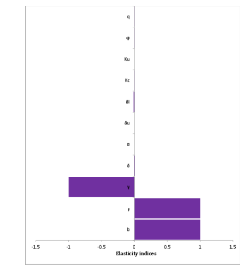
Table 3 shows the sensitivity and elasticity indices obtained with the use of Sage. From the Table one can note that a increase in virus burst size, , and infection rate, , leads to a increase in , whereas a increase in the virus decay rate, , leads to a 1% reduction in . The indices indicate that is most sensitive to virus burst size, infection and decay rates. Figure 1 is a graphical representation of the indices. Figure 2 (a) shows the variation of elasticity of with respect to drug dosage. The figure indicates that increasing the amount of drug infused reduces and thus reduces the number of tumour cells. From the figure we can further infer that values of the drug dosage, , from 40 mg/l to 100 mg/l have a less significant impact on .
| Parameter | Sensitivity index | Elasticity index |
|---|---|---|
4.3. Sensitivity of endemic equilibria
Sensitivity indices of the endemic equilibria is informative about the establishment of the disease. Here, we calculate sensitivity indices of the endemic total tumour density with respect to drug infusion. The gist is to determine the relative change in the tumour equilibria when the amount of drug infused is changed and thus infer the feasible amount of the drug that should be infused. The sensitivity index of the total tumour endemic equilibria with response to drug infusion is given by
| (20) |
where and are calculated from the formula in Equation (47) derived in Appendix D. It is worth noting that the endemic equilibrium of the full chemotherapy model (1)–(6) can not explicitly be determined in terms of the parameters and therefore we numerically computed the equilibrium values.
We used high values of the tumour reproduction rate and virus burst size, that is cells/mm3/day and virions/mm3/day so that . We calculated for several values of . Table 4 shows selected indices for different amounts of the drug infused with their corresponding basic reproduction ratios. Figure 2 (b) is a plot of total tumour sensitivity index with respect to drug infusion. The figure suggests that the feasible amount of drug that should be infused in a patient lies between 50 mg/l and 100 mg/l. This range of values is similar to those inferred from the elasticity indices of .
It is worth noting that when becomes larger than 50 mg/l, the impact of chemotherapy on virotherapy ( and endemic equilibria) becomes less significant. This analysis, nonetheless, does not incorporate the cost for example monetary or treatments side effects. These results will further be confirmed using optimal control theory. In the next section, we set up an optimal control problem to explicitly determine the optimal virus and chemotherapeutic drug dosage combination necessary for tumour eradication in body tissue.
| q (mg/l) | 5 | 10 | 15 | 35 | 50 | 100 |
|---|---|---|---|---|---|---|
5. Optimal control analysis
In this section, we propose and analyze an optimal control problem applied to the chemovirotherapy model to determine the optimal dosage combination of chemotherapy and virotherapy for controlling the tumour. We set the control variables and to respectively be the supply of viruses from an external source of the drug dosage, which are then incorporated into the model system’s equations (3) and (6) to obtain the following control system. For model tractability, we ignore the immune responses.
| (21) |
5.1. The optimal control problem
We wish to determine the optimal combination of controls that will be adequate to minimize the total tumour density () together with the cost of the treatment and negative side effects over a fixed time period. The optimization problem under consideration is to minimise the objective functional:
| (22) |
where is the termination time of the treatment, subject to the control system (5). The two control functions and are assumed to be bounded and Lebesgue integrable. We thus seek an optimal control pair such that:
| (23) |
where is the control set defined by:
where is the maximum number of viruses body tissue can contain and is the maximum tolerated drug dose. These may as well be viewed as the maximum amounts a patient can financially afford. The lower bounds for and correspond to no treatment. Here, it is important to note that the balancing factors and in the objective functional (22) are the relative measures of both the cost required to implement each of the associated controls as well as the negative sides effects due to the treatment.
5.2. Existence of an optimal control pair
We examine sufficient conditions for the existence of a solution to the quadratic optimal control problem.
Proposition 5.
There exists an optimal control pair with a corresponding solution (, , , ) to the model system (5) that minimizes over .
Proof.
The proof of Proposition 5 is based on Theorem 4.1 in Chapter III of Fleming and Rishel [16]. The necessary conditions for existence are stated and verified as follows.
-
(1)
The set of all solutions to the control system (5) and its associated initial conditions and the corresponding control functions in is non-empty.
-
(2)
The control system can be written as a linear function of the control variables with coefficients dependent on time and state variables.
-
(3)
The integrand in the objective functional in Equation (5) is convex on .
The right hand sides of the control system (5) are and bounded below and above (see Appendix A), thus the solutions to the state equations are bounded. It therefore follows from the Picard–Lindelöf theorem [44] that the system is Lipschitz with respect to the state variables. Thus, condition (1) holds. It can be seen from the control system (5) that the right hand sides are linearly dependent of and . Thus, condition (2) also holds. To establish condition (3), we notice that the integrand in the objective functional (5) is convex because it is quadratic in the controls. ∎
5.3. Optimal control characterization
In this section, we characterize the optimal controls which gives the optimal levels for the various control measures and the corresponding states (, , , ). The necessary conditions for the optimal controls are obtained using the Pontryagin’s Maximum Principle [40]. This principle converts the model system (5) into a problem of minimizing pointwise a Hamiltonian, , with respect to and as detailed below.
Proposition 6.
Let and . If is an optimal control pair, then there exists a non-trivial vector
satisfying the following:
| (24) | ||||
with transversality conditions
| (25) |
and optimal controls:
| (26) |
Proof.
The Lagrangian and Hamiltonian for the optimal control system (5) are respectively given by:
| (27) |
and
| (28) |
We thus obtain Equation (24) using the Pontryagin’s maximum principle from
| (29) | ||||
The transversality conditions are as given in Equation (25) since all states are free at . The Hamiltonian is maximized with respect to the controls at the optimal control . Therefore is differentiated with respect to and on , respectively, to obtain
Thus, solving for and on the interior sets gives
By standard control arguments involving the bounds on the controls, , we conclude that:
| (30) |
∎
5.4. The optimality system
6. Numerical simulations
In this section, we discuss the numerical solutions of both the chemovirotherapy model equations (1)–(6) and the optimal control problem defined in Section 5.4. We also outline the parameter choices and the initial conditions. We use parameter values in Table 2 to solve model equations and the optimality system. The numerical solutions of the model equations are illustrated using MATLAB, while the optimality system was solved using a fourth order Runge–Kutta iterative method.
6.1. Parameter values and initial conditions
Some of the parameter values were obtained from fitted experimental data for untreated tumours and virotherapy in mice [4] and others from biological facts in the literature. A tumour nodule can contain about tumour cells [45]. The carrying capacity is therefore considered to be cells per . In vivo experiments estimate the intrinsic rate of growth to be day-1 [6]. We consider the number of viruses produced per day, , to be in the range virions [11]. The amount of drug infused in body tissue, , is considered to be milligrams per day and the decay rate, , to be milligrams per day, values which conform to cancer pharmacokinetic studies [10, 34]. Since infected tumour cells multiplication is enhanced by the oncolytic virus replication, the tumour cells lysis, , is considered to be greater than that for uninfected tumour cells (see Ref [38]). We considered a virus-specific immune response rate, , of day-1 [9]. Both virus and tumour specific immune decay rates are assumed to be day-1, given the fact that their lifespan is less than 100 days [26, 31]. The tumour-specific production rate was estimated at cells per mm3 per day [18, 26]. In all our simulations, unless stated otherwise, we considered the initial concentrations cells per mm3, cells per mm3, virions per mm3, cells per mm3, cells per mm3 and g/ml with a high percentage of untreated tumour cell count to require treatment.
6.2. Chemovirotherapy model
(a)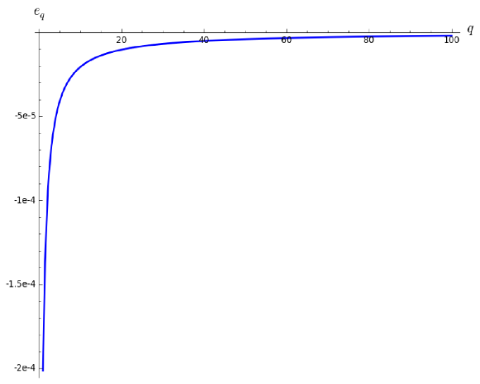
|
(b)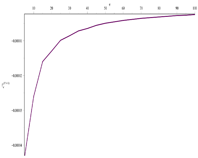
|
a 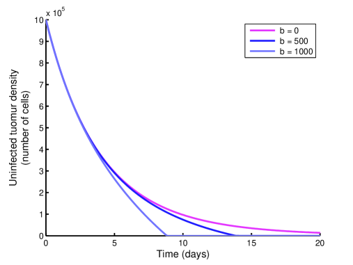
|
b 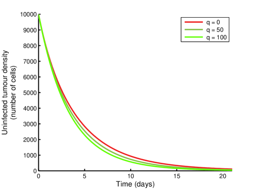
|
a 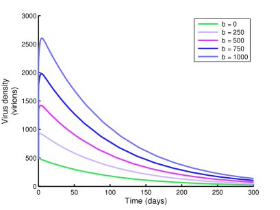
|
b 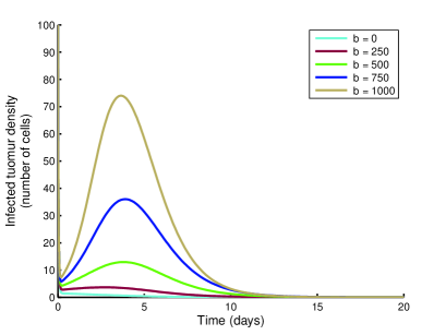
|
a 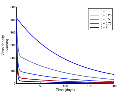
|
b 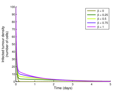
|
Figures 3 (a)&(b) are respectively plots of the uninfected tumour density for different virus and drug doses. Both figures depict that an increase in the virus burst size () and drug dose () reduces the tumour density. In Figure 3 (a), without virotherapy, that is virions, the tumour is depleted in about 10 days whereas without chemotherapy, that is milligrams per day, it takes about 20 days.
Figures 4 and 5 (a)&(b) respectively show the effect of virus burst size on the virus and infected tumour cell densities. Both figures show that the densities with increasing burst size and infection rate. From Figure, for example 4, an increase of from 250 to 500 virions led to an increase of the virus number to about from , in the first 100 days.
Figure 5 (a)&(b) show that increasing virus infection rate, , reduces the virus density and increases the infected tumour density. For example from Figure 5 (a), an increase in from 0 to 1 cells per mm3 per day led to a reduction by about 100 viruses from 120 whereas it led to an increase by about 10 viruses in the first day, from 0 as seen in Figure 5 (b).
6.3. Optimal control problem
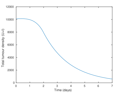
Figure 6 is a plot of total tumour density of the optimal control solution to the problem formulated in Section 5. It shows the tumour density being reduced by the combinational therapy treatment to a very low state in less than a week.
Figures 7 (a)&(b) represent the optimal controls and . The figures suggest that the optimal values of the number of viruses and drug concentration that yields efficient combination therapy are half their maximal dosages and .
(i)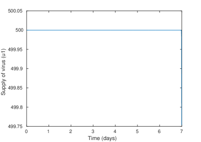
|
(ii)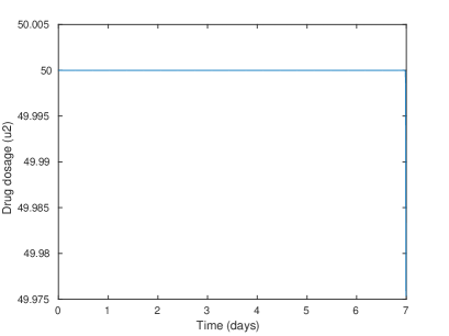
|
7. Conclusion
Successful cancer treatment often requires a combination of treatment regimens. Recently, combined oncolytic virotherapy and chemotherapy has been emerging as a promising, effective and synergetic cancer treatment. In this paper we consider a combination therapy with chemotherapy and virotherapy to investigate how virotherapy could enhance chemotherapy. To this end, we developed a mathematical model and an optimal control problem to determine the optimal chemo-virus combination to eradicate a tumour. We firstly validated the model’s plausibility by proving existence, positivity and boundedness of the solutions. We analysed the model in four scenarios: without treatment, with chemotherapy, with oncolytic virotherapy alone, and with combined chemotherapeutic drug and virus therapy. A basic reproduction number for the infection of the tumour cells was calculated to analyse the model’s tumour endemic equilibrium. Furthermore, sensitivity and elasticity indices of the basic reproduction number and tumour endemic equilibria with respect to drug infusion were calculated. The optimal control problem was solved using the Pontryagin’s Maximum Principle. Numerical solutions to the proposed model were carried out to illustrate the analysis results. Similarly, numerical solutions to the optimal control problem were carried out to identify the optimal dosages for the minimization of the chemo-virus combination. Model analysis and simulations suggest the following results.
The stability analysis showed that a tumour can grow to its maximum size in a case where there is no treatment. It also demonstrated that chemotherapy alone is capable of clearing tumour cells provided that the drug efficacy is greater than the intrinsic tumour growth rate. This can be evidenced in a study by Dasari and Tchounwou [14] and references therein. Furthermore, the result emphasised that if the chemotherapeutic drug’s efficacy is high enough but with a toxic drug then the tumour cannot be eliminated. If, however, the drug is not toxic, then a dosage which is not larger than the maximum tolerated dose can be given while still allowing for a stability condition of the tumour free equilibrium, thus eliminating the tumour.
In the case of virotherapy alone, stability analysis revealed that virotherapy on its own may not clear tumour cells but rather highly enhances chemotherapy in destroying tumour cells. Several clinical and experimental studies for example [35, 8, 20, 41] confirm this result. In a review of clinical studies by Binz and Ulrich [8], it is stated that phase II/III clinical trials on combining adenovirus H101 with a chemotherapeutic drug, cisplatin and 5-fluorouracil, leads to a 40% improvement compared to chemotherapy alone for the treatment of patients with head and neck cancer. Adenovirus Ad-H101 was consequently approved for the treatment of head and neck cancers in China and recently in the United states after phase III clinical trials showed a 72–79% response rate for the combination of the virus with 5-fluorouracil compared to a 40% with chemotherapy alone [19].
Sensitivity analysis and elasticity indices of the basic reproduction ratio indicated that successful chemovirotherapy is highly dependent on the virus burst size and its infection rate as well as on the drug infusion and its decay rates. Larger virus burst size and higher replication rates lead to a lower tumour concentration. Whereas, low decay and high doses of the drug that the body can tolerate lead to better treatment results. Sensitivity analysis of both the basic reproduction ratio and model equilibria suggested the feasible drug infusion to be between 50 and 100 milligrams per litre. The effect of virus burst size and infection rates in determining the success of virotherapy have extensively been confirmed in recent mathematical studies (see for example [29, 47, 13]). Nonetheless, the right dose of chemotherapy treatment has always been a question and a concern to both clinicians and mathematicians alike [25, 17]. In this study, optimal control results further indicated that of the maximum drug and virus tolerated dosages (MTDs) optimize chemovirotherapy.
In addition, numerical simulations suggested that with the use of both chemotherapy and virotherapy, a tumour may be eradicated in less than a month. We know that this is not realistic for human cancers and is strictly based on the experimental data used in the numerics. Simulations further showed that a successful combinational therapy of cancer drugs and viruses is mostly dependent on virus burst size, infection rate and the amount of drugs supplied into a patient’s body which is in agreement with recent studies [29, 47, 13].
The mathematical model we developed in this study is a simple one, for example, it considers the cell densities to only be time dependent. It is therefore imperative for further studies to incorporate more biological aspects like spatial variation of the cell concentrations. Another facet would be to investigate the effect of toxicity of both viruses and the drug on normal body tissue. The key to improving combined virotherapy and chemotherapy lies in quantifying the dependence of treatment outcome on immune stimulation. Another extension to this model, would be to include other subpopulations of the immune system. Nevertheless, the results here emphasise the treatment characteristics that are vital in combining drugs and viruses to treat cancer and an optimal drug and virus dosage is suggested.
Appendix A Appendix A
A.1. Proof of Theorem 3.1(i) on the existence and uniqueness of model solutions
Proof.
A.2. Proof of Theorem 3.1(ii)&(iii) on positivity and boundedness
Proof.
The solution to Equation (6) is given by
Let the model equations (1)-(5) be written in the form . The functions on the right hand side of Equations (1)–(5) have the property of
where . Thus, it follows from Proposition A.1 in [46] that
and thus the model solutions are positive and bounded for positive initial values . ∎
A.3. Proof of Theorem 3.1(iv) on positive invariance
Proof.
The proof directly follows from proofs of Theorems 3.1 (i)–(iii). ∎
Appendix B Appendix B
B.1. Proof of stability of tumour endemic state, , in Proposition 1.
Proof.
Denote where
The characteristic polynomial of the Jacobian matrix evaluated at is given by
| (31) |
where and ,
Using Routh–Hurwitz criterion, the endemic steady state, , is locally asymptotically stable if and .
We notice that . This means that if and only if which is equivalent to
With the help of Maple®, we find that
Therefore .
For , we discuss the following cases:
-
(i)
If then .
-
(ii)
If then if and only if which is equivalent to
Using Maple®, we find that
This implies that .
Therefore the endemic steady state, , is locally asymptotically stable. ∎
B.2. Proof of stability of endemic state, , in Proposition 2
Proof.
The characteristic polynomial, , of the Jacobian evaluated at is given by
| (32) | ||||
| (33) | ||||
| (34) | ||||
| (35) |
The conditions for stability of the endemic state, , therefore follow from the Routh–Hurwitz criterion and are stated as:
| (36) |
∎
Appendix C Appendix C
C.1. Proof of conditions for the derivation of
Proof.
Denote with be the set of cell compartments divided into infected cells and uninfected cells . Define to be the set of virus or infection free states:
Let be the input rate of newly infected cells in the compartment. Let and respectively be the input rate of cells by other means and rate of transfer of cells out of a compartment . Thus the system of Equations (1)–(6) take the form
We now proceed to prove the assumptions :
: For each , the functions , and are non-negative and continuous on and continuously differentiable with respect to . From Equations (1)–(6)
| (37) |
Clearly, , and satisfy .
: If , then . Clearly, from (37), if the state variables are all equal to zero, then .
: for . This can be seen from the compartments , and .
: If , then for . At , and are zero, implying that .
: If , then all the eigenvalues of have positive real parts. This can be ascertained from Equation (37). ∎
C.2. Proof of Theorem 4.1
Proof.
Appendix D Appendix D
D.1. Elasticity indices of
| (39) | ||||
where
D.2. Elasticity indices of endemic equilibrium.
Consider a system of differential equations dependent on a parameter
| (40) |
where
At equilibrium point satisfies . Differentiating with respect to , one obtains
This implies that
Multiplying both sides with the diagonal matrix, , matrix
The sensitivity indices of the steady state variables at equilibrium with respect to a parameter are therefore given by
| (47) |
Acknowledgments
Joseph Malinzi was jointly supported by the University of Pretoria and DST/NRF SARChI Chair in Mathematical Models and Methods in Bioengineering and Biosciences.
Amina Eladdadi and K.A. Jane White would like to acknowledge and thank the UK-QSP Network (Grant-EP/N005481/1) for their financial support to attend the QSP-1st Problem Workshop and collaborate on this research.
Torres was supported by FCT through CIDMA, project UID/MAT/04106/2013, and TOCCATA, project PTDC/EEI-AUT/2933/2014, funded by FEDER and COMPETE 2020.
References
- [1] (MR2830838) [10.4236/am.2011.21015] M. Agarwal and A. S. Bhadauria, Mathematical modeling and analysis of tumor therapy with oncolytic virus, Journal of Applied Mathematics, 2 (2011), 131–140.
- [2] (MR3262662) [10.1007/s40314-013-0083-x] T. Agrawal, M. Saleem and S. Sahu, Optimal control of the dynamics of a tumor growth model with hollings’ type–II functional response, Computational and Applied Mathematics, 33 (2014), 591–606.
- [3] [10.1038/sj.cgt.7701067] M. Alonso, C. Gomez-Manzano, H. Jiang, N. B. Bekele, Y. Piao, W. K. A. Yung, R. Alemany and J. Fueyo, Combination of the oncolytic adenovirus ICOVIR-5 with chemotherapy provides enhanced anti-glioma effect in vivo, Journal of Cancer Gene Therapy, 14 (2007), 756–761.
- [4] (MR2948550) [10.1016/j.jtbi.2008.01.016] Z. Bajzer, T. Carr, K. Josic, S. J. Russell and D. Dingli, Modeling of cancer virotherapy with recombinant measles viruses, Journal of Theoretical Biology, 252 (2008), 109–122.
- [5] M. Bartkowski, S. Bridges, P. Came, H. Eggers, P. Fischer, H. Friedmann, M. Green, C. Gurgo, J. Hay, B. D. Korant et al., Chemotherapy of viral infections, vol. 61, Springer Science & Business Media, 2012.
- [6] [10.1371/journal.pcbi.1003800] S. Benzekry, C. Lamont, A. Beheshti, A. Tracz and J. M. L. Ebos, Classical mathematical models for description and prediction of experimental tumor growth, PLoS Comput Biol 10 (2014), no. 8, e1003800.
- [7] M. Bertau, E. Mosekilde and H. V. Westerhoff, Biosimulation in drug development, John Wiley & Sons, 2008.
- [8] [10.2147/OV.S54780] E. Binz and L. M. Ulrich, Chemovirotherapy: Combining chemotherapeutic treatment with oncolytic virotherapy, Oncolytic Virotherapy, 4 (2015), 39–48.
- [9] [10.1182/blood-2016-01-628982] C.M. Bollard and H.E. Heslop, T cells for viral infections after allogeneic hematopoietic stem cell transplant, Blood 127 (2016), no. 26, 3331–3340.
- [10] [10.1200/JCO.2010.29.5055] G. J. Bostol and S. Patil, Carboplatin in clinical stage I seminoma: too much and too little at the same time, Journal of Clinical Oncology, 29 (2011), 949–952.
- [11] T. D. Brock, The emergence of bacterial genetics, Cold Spring Harbor Laboratory Press Cold Spring Harbor, New York, 1990.
- [12] [10.7326/0003-4819-99-6-823] R. W. Carlson and B. I. Sikic, Continuous infusion or bolus injection in cancer chemotherapy, Annals of Internal Medicine, 99 (1983), 823–833.
- [13] (MR2928374) [10.1080/17513758.2011.613486] J. Crivelli, J. Földes, P. Kim and J. Wares, A mathematical model for cell cycle-specific cancer virotherapy, Journal of Biological Dynamics, 6 (2012), 104–120.
- [14] [10.1016/j.ejphar.2014.07.025] S. Dasari and P. Tchounwou, Cisplatin in cancer therapy: molecular mechanisms of action, European Journal of Pharmacology, 740 (2014), 364–378.
- [15] (MR2566932) [10.1080/17486700802216301] L. de Pillis, K. R. Fister, W. Gu, C. Collins, M. Daub, D. Gross, J. Moore and B. Preskill, Mathematical model creation for cancer chemo-immunotherapy, Journal of Computational and Mathematical Methods in Medicine, 10 (2009), 165–184.
- [16] (MR0454768) W. Fleming and R. Rishel, Deterministic and stochastic optimal control, vol. 1, Springer Science & Business Media, 2012.
- [17] [10.1016/0002-9343(80)90472-6] E. Frei III and G. P. Canellos, Dose: a critical factor in cancer chemotherapy, The American Journal of Medicine, 69 (1980), 585–594.
- [18] [10.1038/ni.2703] T. Gajewski, H. Schreiber and Y. Fu, Innate and adaptive immune cells in the tumor microenvironment, Nature Immunology, 14 (2013), 1014–1022.
- [19] [10.1093/jnci/djj111] K. Garber, China approves world’s first oncolytic virus therapy for cancer treatment, Journal of the National Cancer Institute, 98 (2006), 298–300.
- [20] [10.1038/nature01112] V. Groh, J. Wu, C. Yee and T. Spies, Tumour-derived soluble MIC ligands impair expression of nkg2d and T-cell activation, Journal of Nature, 419 (2002), 734–738.
- [21] [10.3389/fonc.2017.00195] A. Howells, G. Marelli, N. Lemoine and Y. Wang, Oncolytic viruses-interaction of virus and tumor cells in the battle to eliminate cancer, Frontiers in Oncology, 7 (2017), 195.
- [22] [10.1038/sj.mt.6300108] E. Kelly and S. J. Russel, History of oncolytic viruses: genesis to genetic engineering, Journal of Molecular Therapy, 15 (2007), 651–659.
- [23] (MR3276718) [10.1016/j.amc.2014.10.009] S. Khajanchi and S. Banerjee, Stability and bifurcation analysis of delay induced tumor immune interaction model, Applied Mathematics and Computation, 248 (2014), 652–671.
- [24] [10.1007/s002850050127] D. Kirschner and J. Panetta, Modeling immunotherapy of the tumor–immune interaction, Journal of Mathematical Biology, 37 (1998), 235–252.
- [25] [10.1098/rsif.2017.0150] A. Konstorum, A. Vella, A. Adler and R. Laubenbacher, Addressing current challenges in cancer immunotherapy with mathematical and computational modeling, The Royal Society Interface 14 (2017), no. 131, 20170150.
- [26] [10.3389/fcimb.2014.00177] D. Le, J. Miller and V. Ganusov, Mathematical modeling provides kinetic details of the human immune response to vaccination, Frontiers in Cellular and Infection Microbiology, 4 (2015), 177.
- [27] T. C. Liau, E. Galanis and D. Kirn, Clinical trial results with oncolytic virotherapy: a century of promise, a decade of progress, Journal of Nature Clinical Practice Oncology, 4 (2007), 101–117.
- [28] (MR2181302) [10.1016/j.mcm.2004.09.008] W. Liu and H. I. Freedman, A mathematical model of vascular tumor treatment by chemotherapy, Journal of Mathematical and Computer Modelling, 42 (2005), 1089–1112.
- [29] (MR3733435) [10.1080/17513758.2017.1328079] J. Malinzi, A. Eladdadi and P. Sibanda, Modelling the spatiotemporal dynamics of chemovirotherapy cancer treatment, Journal of Biological Dynamics, 11 (2017), 244–274.
- [30] (MR3327996) [10.1016/j.mbs.2015.01.015] J. Malinzi, P. Sibanda and H. Mambili-Mamoboundou, Analysis of virotherapy in solid tumor invasion, Journal of Mathematical Biosciences, 263 (2015), 102–110.
- [31] [10.1080/2162402X.2014.1002720] S. Nayar, P. Dasgupta and C. Galustian, Extending the lifespan and efficacies of immune cells used in adoptive transfer for cancer immunotherapies–a review, Oncoimmunology, 4 (2015), e1002720.
- [32] [10.3389/fonc.2014.00145] A. Nguyen, L. Ho and Y. Wan, Chemotherapy and oncolytic virotherapy: advanced tactics in the war against cancer, Frontiers in Oncology, 4 (2014), 145.
- [33] [10.1186/1745-6150-1-6] A. S. Novozhilov, F. S. Berezovskaya, E. V. Koonin and G. P. Karev, Mathematical modeling of tumor therapy with oncolytic viruses: regimes with complete tumor elimination within the framework of deterministic models, Biology Direct, 1 (2006), 1–18.
- [34] [10.1200/JCO.2009.26.4655] R. T. D. Oliver, G. M. Mead, G. J. Rustin, J. S. Gordon, J. K. Joffe, N. Aass, R. Coleman, P. P. R. Gabe and S. P. Stenning, Randomized trial of carboplatin versus radiotherapy for stage I seminoma: mature results on relapse and contralateral testis cancer rates in MRC TE19/EORTC 30982 study (ISRCTN27163214), Journal of Clinical Oncology, 29 (2011), 957–962.
- [35] [10.1038/mt.2009.283] P. K. Ottolino, J. S. Diallo, B. D. Lichty, J. C. Bell and J. A. McCart, Intelligent design: combination therapy with oncolytic viruses, Journal of Molecular Therapy, 18 (2010), 251–263.
- [36] (MR2300333) [10.3934/dcdsb.2007.8.229] R. Ouifki and G. Witten, A model of HIV-1 infection with HAART therapy and intracellular delays, Discrete and Continuous Dynamical Systems Series B, 8 (2007), 229–240.
- [37] (MR1950733) [10.1016/S0895-7177(02)00227-3] S. T. R. Pinho, H. I. Freedman and F. K. Nani, A chemotherapy model for the treatment of cancer with metastasis, Journal of Mathematical and Computer Modelling, 36 (2002), 773–803.
- [38] (MR2987754) S. T. R. Pinho, D. S. Rodrigues and P. F. A. Mancera, A mathematical model of chemotherapy response to tumour growth, Canadian Applied Math Quarterly, 19 (2011), 369–384.
- [39] (MR2969876) [10.1016/j.nonrwa.2012.07.034] S. Pinho, R. A. F.S. Bacelar and H. Freedman, A mathematical model for the effect of anti-angiogenic therapy in the treatment of cancer tumours by chemotherapy, Nonlinear Analysis: Real World Applications, 14 (2013), 815–828.
- [40] (MR0186436) L. S. Pontryagin, V. G. Boltyanskii, R. V. Gamkrelidze and E. F. Mishchenko, The mathematical theory of optimal processes, Translated by D. E. Brown, A Pergamon Press Book. The Macmillan Co., New York, 1964.
- [41] [10.2147/OV.S66083] G. R. Simpson, K. Relph, K. Harrington, A. Melcher and H. Pandha, Cancer immunotherapy via combining oncolytic virotherapy with chemotherapy: recent advances, Oncolytic Virotherapy, 5 (2016), 1–13.
- [42] R.J. de Boer, Modeling population dynamics: A graphical approach, Utrecht University, 2018.
- [43] [10.1038/nbt.2287] S. J. Russel, K. W. Pengl and J. C. Bell, Oncolytic virotherapy, Journal of Nature Biotechnology, 30 (2012), 658–670.
- [44] (MR2858149) [10.1017/CBO9781139057707] B. J. Schroers, Ordinary differential equations: a practical guide, Cambridge University Press, 2011.
- [45] [10.1002/jso.2930600216] J. S. Spratt, J. S. Meyer and J. A. Spratt, Rates of growth of human solid neoplasms: Part I, Journal of Surgical Oncology, 60 (1995), 137–146.
- [46] (MR1993355) H. Thieme, Mathematics in population biology, Princeton University Press, NJ, 2003.
- [47] (MR2811015) [10.3934/mbe.2011.8.841] J. P. Tian, The replicability of oncolytic virus: defining conditions in tumor virotherapy, Journal of Mathematical Biosciences and Engineering, 8 (2011), 841–860.
- [48] [10.1038/nrc1629] S. D. Undevia, A. G. Gomez and M. J. Ratain, Pharmacokinetic variability of anticancer agents, Nature Reviews Cancer, 5 (2005), 447–458.
- [49] [10.1038/gt.2010.103] G. Ungerechts, M. E. Frenzke, K. C. Yaiw, T. Miest, P. B. Johnston and R. Cattaneo, Mantle cell lymphoma salvage regimen: synergy between a reprogrammed oncolytic virus and two chemotherapeutics, Gene Therapy, 17 (2010), 1506–1516.
- [50] [10.1016/0898-1221(94)00179-0] J. R. Usher, Some mathematical models for cancer chemotherapy, Journal of Computers & Mathematics with Applications, 28 (1994), 73–80.
- [51] US Food and Drug Administration and others, FDA approves first-of-its-kind product for the treatment of melanoma. press release. October 27, 2015.
- [52] (MR1950747) [10.1016/S0025-5564(02)00108-6] P. van den Driessche and J. Watmough, Reproduction numbers and sub-threshold endemic equilibria for compartmental models of disease transmission, Mathematical Biosciences, 180 (2002), 29–48.
- [53] (MR3028443) [10.1016/j.apm.2012.12.004] Y. Wang, J. P. Tian and J. Wei, Lytic cycle: A defining process in oncolytic virotherapy, Journal of Applied Mathematical Modelling, 37 (2013), 5962–5978.
- [54] D. Wodarz, Viruses as antitumor weapons defining conditions for tumor remission, Journal of Cancer Research, 61 (2001), 3501–3507.
- [55] M. Yoshimori, H. Ookura, Y. Shimada, T. Yoshida, N. Okazaki, M. Yoshino and D. Saito, [continuous infusion of anti-cancer drug with balloon infusors], Gan to Kagaku Ryoho. Cancer & Chemotherapy, 15 (1988), 3121–3125.
Submitted 27-March-2018; revised 04-July-2018; accepted 10-July-2018.