The Pristine Survey IV: Approaching the Galactic metallicity floor with the discovery of an ultra metal-poor star

Abstract

The early Universe presented a star formation environment that was almost devoid of heavy elements. The lowest metallicity stars thus provide a unique window into the earliest Galactic stages, but are exceedingly rare and difficult to find. Here we present the discovery of an ultra-metal-poor star, Pristine_221.8781+9.7844, using narrow-band Ca H&K photometry from the Pristine survey. Follow-up medium and high-resolution spectroscopy confirms the ultra-metal-poor nature of Pristine_221.8781+9.7844  ([Fe/H] = $-$4.66 $\pm$ 0.13 in 1D LTE) with an enhancement of 0.3$-$0.4 dex in $\alpha$-elements relative to Fe, and an unusually low carbon abundance. We derive an upper limit of A(C) = 5.6, well below typical A(C) values for such ultra metal-poor stars. This makes Pristine_221.8781+9.7844  one of the most metal-poor stars; in fact, it is very similar to the most metal-poor star known (SDSS J102915+172927). The existence of a class of ultra metal-poor stars with low(er) carbon abundances suggest that there must have been several formation channels in the early Universe through which long-lived, low-mass stars were formed.

1 Introduction

The search for the most metal-poor stars has been compared to finding a needle in a haystack. In a typical halo field, only one in $\sim$80,000 stars is expected to have [Fe/H]$<-4$ (Youakim et al., 2017). Although much effort has been devoted to the discovery and study of extremely, ultra, and hyper metal-poor stars with [Fe/H] $<-3.0$, [Fe/H] $<-4.0$, and [Fe/H]$<-5.0$, respectively, their overall numbers remain small. Still, these stars paint a fascinating picture about chemical enrichment in the very early Galaxy and the physics of star formation in environments that were mostly devoid of metals.

The first stars that formed in the Universe necessarily contained only hydrogen, helium and traces of lithium. However, no star with such a primordial composition has been observed to date. As such, it is heavily debated whether long-lived stars (of lower mass) were formed in this epoch. Theoretical studies point out that, in gas environments devoid of heavier elements, cooling is more problematic and therefore proto-stars will be heavier and shorter lived. It is unclear, though, if in the fragmentation of the proto-stellar cloud any stars with masses lower than one solar mass could be formed that would have lifetimes similar to the age of the Universe (see Bromm, 2013; Greif, 2015, and references therein).

In addition to cooling through metallic atomic lines, it is thought that dust grains can be an important cooling mechanism in very metal-poor environments, bringing down the critical metallicity to allow cooling in lower mass proto-stellar clouds (see e.g., Omukai, Schneider & Haiman, 2008; Schneider et al., 2012a, b; Chiaki, Tominaga & Nozawa, 2017).

There are presently 12 stars known to have intrinsic iron-abundances below [Fe/H] = $-$4.5 (Christlieb, Wisotzki & Graßhoff, 2002; Frebel et al., 2005; Norris et al., 2007; Caffau et al., 2011a; Norris et al., 2012; Keller et al., 2014; Hansen et al., 2014; Allende Prieto et al., 2015; Frebel et al., 2015; Bonifacio et al., 2015; Caffau et al., 2016; Bonifacio et al., 2018a; Aguado et al., 2018a, b). The SkyMapper Southern Sky Survey star SMSS J031300.36-670839.3, which is the current record holder amongst iron-poor stars at [Fe/H] $<-7.0$, shows a very high carbon abundance of [C/Fe]$>5$ (Nordlander et al., 2017). Based on the handful of stars found in the ultra metal-poor regime, this seems very typical for this metallicity regime; almost all ultra iron-poor stars show a very high carbon abundance (see e.g., the compilations in Norris et al., 2013; Frebel et al., 2015; Aguado et al., 2017). It has been noted that there seems to be a trend with increasing carbon-to-iron ratio as [Fe/H] decreases, and for many of the most iron-poor stars, the absolute abundance of carbon lies around a value of A(C) $\sim$ 6.5 (Spite et al., 2013; Yoon et al., 2016). While the main focus in classification diagnostics has been on the (more readily measureable) carbon abundance, other light elements, such as nitrogen, oxygen, and sodium, are also often greatly enhanced in these stars with respect to solar [X/Fe] abundance ratios. However, there are certainly stars observed that do not follow this trend. The most metal-poor star known today is the ultra metal-poor star SDSS J102915+172927, that was shown not to be highly carbon-enhanced, but instead to have A(C) $<$ 4.2 at [Fe/H] $\sim$ –5.0. This star, as well as some other stars with only mild carbon enhancements (e.g., Norris et al., 2012), suggest that there might be multiple formation routes for ultra metal-poor stars, with important consequences for theories of early star formation in the Galaxy. On the other hand, very recently a new hyper iron-poor star, SDSS J0815+4729, has been discovered showing a extremely high carbon abundance A(C) $\sim 7.7$ dex (Aguado et al., 2018a).

We report here the discovery of Pristine_221.8781+9.7844, an ultra low-metallicity star which belongs to the rare class of objects that have both low [Fe/H] as well as [C/Fe] abundances. This star was discovered thanks to the discriminatory power of narrow-band Ca H&K photometry from the Pristine survey (see Starkenburg et al., 2017; Caffau et al., 2017; Youakim et al., 2017), in combination with broad-band photometry from the Sloan Digital Sky Survey (SDSS, Albareti et al., 2017). The effectiveness of such narrow-band imaging techniques — or, alternatively, very low-resolution prism spectroscopy in this same wavelength region — has been convincingly demonstrated in the past (e.g., Beers, Preston & Shectman, 1985; Anthony-Twarog et al., 1991, 2000; Christlieb, Wisotzki & Graßhoff, 2002; Keller et al., 2007; Murphy et al., 2009; Howes et al., 2015; Koch et al., 2016). The discovery of this new star demonstrates the increasing efficiency with which astronomers are now able to identify “the needles in the haystack”.

In Section 2, we describe the initial selection of this star and the derivation of stellar parameters from photometry and astrometry. In Section 3 we describe the medium-resolution spectrum and its analysis, and in Section 4 the high-resolution spectrum used to study its chemical properties. We calculate the abundances from absorption features in Section 5, and discuss the uncertainties on these measurements due to uncertainties in stellar parameters as well as 3D non-LTE effects. Finally, in Section 6, we show how Pristine_221.8781+9.7844 compares with other stars having similar metallicities.

2 Photometry

2.1 Photometric selection

Pristine_221.8781+9.7844 was first identified in our narrow-band photometric survey Pristine (Starkenburg et al., 2017) as a candidate extremely metal-poor star. It was selected as a candidate for follow-up spectroscopy following the procedure outlined in Youakim et al. (2017), based on its $CaHK$ filter magnitude from the Pristine survey in combination with SDSS broad-band photometry (see Table 1). Its photometric metallicity from Pristine Ca H&K narrow-band photometry and SDSS broad-band photometry (see for a detailed description of the procedure Starkenburg et al., 2017) was estimated to be [Fe/H]$\sim-3.2$, but we note that, at metallicities well below [Fe/H]$=-3$, even the very metallicity sensitive Pristine photometry loses its discriminative power, and follow-up spectroscopy is therefore needed to determine the final metallicity of the star and, of course, to establish its overall abundance pattern.

	unit	value	uncertainty	extinction	source
				applied
Right Ascension	(h:m:s J2000)	14:47:30.73	–	–	SDSS
Declination	(d:m:s J2000)	+09:47:03.70	–	–	SDSS
$u_{0}$	(mag)	17.411	0.010	0.100	SDSS
$g_{0}$	(mag)	16.512	0.004	0.078	SDSS
$r_{0}$	(mag)	16.177	0.005	0.054	SDSS
$i_{0}$	(mag)	16.035	0.005	0.040	SDSS
$z_{0}$	(mag)	15.982	0.007	0.030	SDSS
$CaHK_{0}$	(mag)	16.869	0.005	0.093	Pristine
$V_{0}$	(mag)	16.356	0.020	0.072	APASS
$J_{0}$	(mag)	15.145	0.008	0.020	UKIDSS to 2MASS
$H_{0}$	(mag)	14.779	0.011	0.010	UKIDSS to 2MASS
$K_{0}$	(mag)	14.473	0.012	0.008	UKIDSS to 2MASS
proper motion RA	(mas/yr)	$-7.76$	0.11	–	Gaia DR2
proper motion DEC	(mas/yr)	$-0.06$	0.12	–	Gaia DR2
parallax	(mas)	0.119	0.094	–	Gaia DR2
distance	(kpc)	6.9	0.3	–	isochrone fitting + Gaia DR2
log(g)	(dex)	3.5	0.5	–	isochrone fitting + Gaia DR2
$T\rm_{eff}$	(K)	5792	100	–	3D corrected stellar models

Table 1: Position, photometry from SDSS DR13 (Albareti et al., 2017) and Pristine, astrometry from Gaia DR2 (Gaia Collaboration et al., 2018), and adopted stellar parameters for Pristine_221.8781+9.7844.

2.2 Derivation of stellar parameters

Table 1 summarises the photometry for Pristine_221.8781+9.7844 that is available from SDSS DR13 (Albareti et al., 2017). Comparison of the SDSS colours to the most metal-poor MESA isochrones (Paxton et al., 2011; Choi et al., 2016; Dotter, 2016) suggest that the star is either a sub-giant of log(g) $\sim$ 3.5 at a distance of $\sim$7 kpc, or on the main-sequence with log(g) $\sim$ 4.5 at a distance of $\sim$1.2 kpc. For the probability distribution function of the two solutions, shown by a blue line in Figure 1, we have included the assumption that the star is old (age $>$ 11 Gyr), but the precise age is treated by a flat prior. Additionally, we have assumed that this extremely metal-poor star follows the halo density distribution described as a single power-law with $n=-3.4$ (e.g., Kafle et al., 2014, this is an average value, we have verified that the results are robust to a change in slope from $-2$ to $-4.5$). The resulting probability distribution favours the sub-giant solution for Pristine_221.8781+9.7844 by a factor 8, which is indicative, but can not be taken as a definitive answer. A careful fitting of the Balmer line series brought no clarity in this issue, as no combination of Teff and log(g) simultaneously provided a good fit to the full Balmer series. However, this degeneracy is broken by the parallax measurements from the ESA Gaia satellite released in Gaia DR2 (Gaia Collaboration et al., 2018) presenting a parallax of 0.119 $\pm$ 0.094 mas, thereby favouring the sub-giant solution with extremely high probability (99.7%, see Figure 1, details of the method to be published in Sestito et al., in prep.), and constraining the distance to Pristine_221.8781+9.7844 to 6.9 $\pm$ 0.3 kpc.

Using ($g_{0}-z_{0}$) = 0.530 and log(g) = 3.5, we derive $T\rm_{eff}$ from an interpolation between the 3D-corrected ATLAS colours given in Bonifacio et al. (2018b), which gives our final adopted value of 5792 K. For comparison, we would derive $T\rm_{eff}$ = 5805 K from the formula given in Ludwig et al. (2008) for extremely metal-poor stars. The photometric calibration given by Casagrande et al. (2010) yield a consistent result if we convert the SDSS magnitudes to ($V-I$) using the relation from Jordi, Grebel & Ammon (2006). Unfortunately, the available photometry in the infrared bands from 2MASS (Skrutskie et al., 2006) has too large uncertainties to use for reliable effective temperatures. However, we instead use UKIDSS JHK magnitudes (Lawrence et al., 2012) transformed to the 2MASS system and de-reddened using the maps from Schlegel, Finkbeiner & Davis (1998). Using the converted infrared magnitudes and the Johnson V magnitude from APASS (Henden et al., 2012), we apply the infrared flux method (González Hernández & Bonifacio, 2009) to obtain $T\rm_{eff}$ of 5877 $\pm$ 62 K. The method by González Hernández & Bonifacio (2009) is calibrated down to ultra-low metallicities ([Fe/H]$=-4$) and the result is nicely consistent with our derived temperature from optical colours. Finally, we mention that the derived temperature value from Gaia DR2 photometry alone (Andrae et al., 2018) is also consistent although it has significantly larger uncertainties ($T\rm_{eff}$ = 5862${}^{+175}_{-169}$).

The measured proper motion from Gaia DR2 is (pmRA, pmDEC) = ($-7.76\pm 0.11$ mas/yr,$-0.06\pm 0.12$ mas/yr). Taken together with our measured radial velocity of $-$149 $\mathrm{km\,s^{-1}}$ from the spectra (see Section 4), this gives: ($U,V,W$)$=$($-226.4^{+12.2}_{-15.8},-171.6^{+14.1}_{-16.7},17.4^{+11.7}_{-8.4}$) $\mathrm{km\,s^{-1}}$, with respect to the Galactic standard of rest. This 3D velocity is inconsistent with a star co-rotating in the Galactic disk, therefore we can conclude that it is a halo star.

Table 1 summarises the adopted stellar parameters for Pristine_221.8781+9.7844 which will be used in the remainder of this work.

Figure 1: Probability distribution function of the distance of Pristine_221.8781+9.7844. Shown here are the likelihood based on the MESA isochrones alone (blue line), the likelihood based on the Gaia parallax (red line, multiplied by a factor 20 for visibility), and the combined posterior (black line). The sub-giant solution with a distance of $6.9\pm 0.3$ kpc is favoured with a very high confidence level (99.7%).

3 Medium-resolution Spectroscopy

Initially, follow-up medium-resolution spectroscopy was obtained with the Intermediate dispersion Spectrograph and Imaging System (ISIS) (Jorden, 1990) spectrograph on the 4.2m William Herschel Telescope (WHT) at the Observatorio del Roque de los Muchachos on La Palma, Spain. We used the R600B and R600R gratings, the GG495 filter in the red arm, and the default dichroic (5300 Å). The mean FWHM resolution with a one arcsecond slit was R $\sim$2400 in the blue arm. The observations were carried out over the course of a five night observing run (15–19 July, 2017, Programme C31). Eight exposures of 1800 s each were taken, although unfortunately with fairly high particle counts in the air and some of them at high airmass. A standard data reduction procedure including bias subtraction, flat-fielding, and wavelength calibration using CuNe and CuAr lamps was performed with the onespec package in IRAF. The final signal-to-noise ratio of the average reduced spectrum is S/N $\sim$180 at 4500 Å.

Figure 2 shows the spectrum, which is characterised by very few metal absorption lines and a very weak Ca II K line, which has an equivalent width of only $\sim$450 mÅ. The Ca II H line, to the immediate right, looks much stronger in comparison because it is blended with the Balmer H$\epsilon$ line.

Figure 2: Top panel: The medium-resolution spectrum for Pristine_221.8781+9.7844 as observed with WHT/ISIS. The main lines are labelled and one can clearly see that the medium-resolution spectrum is dominated by the H Balmer series. The weaker Ca II line is the Ca II K line, the Ca II H line is blended with H$\epsilon$. Bottom panel: The same spectrum, but now normalised by a running mean by the FERRE code and with the best-fit synthetic spectrum – with the same normalisation – overplotted in red.

3.1 Analysis

To derive stellar parameters and chemical abundances, a grid of synthetic spectra was computed with the ASS$\epsilon$T package (Koesterke, Allende Prieto & Lambert, 2008) which uses the Barklem codes (Barklem, Piskunov & O’Mara, 2000a, b) to describe the broadening of the Balmer lines. This grid is identical to that used and made publicly available by Aguado et al. (2017). The model atmospheres were computed with the same Kurucz codes and methods described by Mészáros et al. (2012). The abundance of $\alpha$-elements was fixed to [$\alpha$/Fe] = +0.4, and the limits of the grid were taken to be $-6<$ [Fe/H] $<-2$, $-1<$ [C/Fe] $<+5$, 4750K $<T_{\rm{eff}}<$ 7000K and 1.0 $<$ log g $<$ 5.0, with an assumed microturbulence of 2 km s^-1. We search for the best fit model using FERRE (Allende Prieto et al., 2006) by simultaneously deriving surface gravity, metallicity and carbon abundance. The observed and synthetic spectra were both normalized using a running-mean filter with a width of 30 pixels (about 10 Å), see for the fit the lower panel of Figure 2.

3.2 Results

The analysis with FERRE returns a best-fit value of [Fe/H] = $-$4.45 $\pm$ 0.21, an effective temperature of T_eff = 5871 $\pm$ 80 K, and a log(g) of 4.39 $\pm$ 0.5. We note that, in metal-poor stars, the surface gravity is the most difficult parameter to derive from medium-resolution spectroscopy. In this case FERRE has converged on the main-sequence solution for the evolutionary stage of the star, which is not supported by the Gaia DR2 parallax as shown in Figure 1. The metallicity derivation is however not very sensitive to the correct log(g) value (see also Section 5.1). In addition, we note that adopting a different microturbulence value only marginally changes the derived parameters, well below the level of the given uncertainties (see Section 5.1 and more detailed tests in Aguado et al., 2018a).

Due to the extreme weakness of most of the absorption lines, most information for the metallicity determination in this spectrum comes from the Ca II K line. Upon close inspection, though, this line looks slightly asymmetric, indicating that at this resolution the Ca ii K line is blended with an interstellar Ca absorption feature and that the actual metallicity is even lower. A high-resolution spectrum, as discussed in Section 4, is needed to resolve these two features.

Figure 3: Synthetic spectra with $T\rm_{eff}$ = 5792 K, log(g) = 3.5, [Fe/H] = -4.66 and different carbon abundances compared in the region of the carbon G-band to the low-resolution spectrum from of Pristine_221.8781+9.7844 from the WHT. All synthetic spectra are smoothed to resolving power 2400 and the N and O abundances are changed in lockstep with the carbon abundance. For this purpose, the WHT spectrum has been continuum normalised locally (on a scale a little larger than the region shown here) by a linear function only to avoid any dipping of the continuum normalising function into the broad G-band features. The inset zooms in on the wavelength region most sensitive to the CH features.

As illustrated in Figure 2, the absence of a carbon-band around 4300 Å is a striking feature of the medium-resolution spectrum of Pristine_221.8781+9.7844. This suggests that this star might be very carbon-poor in comparison to stars of similar [Fe/H]. In Figure 3, we compare this high S/N medium-resolution spectrum with synthetic spectra of different carbon abundances in the region of the molecular G-band sensitive mostly to the CH molecule. The synthetic spectra are produced using MARCS (Model Atmospheres in Radiative and Convective Scheme) stellar atmospheres and the Turbospectrum code (Alvarez & Plez, 1998; Gustafsson et al., 2008; Plez, 2008) and adopt the stellar parameters from Table 1. It is assumed that N and O change in lockstep with C, keeping [C/N] and [C/O] at the solar values, although we verified that changes in this assumption do not significantly influence the derived abundance. A subsequent analysis using instead ATLAS9 atmosphere models and the MOOG synthetic spectrum code to check for systematic effects yielded the same results. Extra care was taken in normalizing the observed spectrum by the continuum. To prevent any dipping of the continuum fitting into the broad carbon features, this spectrum was normalized locally (on a scale slightly larger than the wavelength range shown in Figure 3) by a linear relation only. It is clear that the spectrum is not carbon-enhanced to the level of A(C) = 6.0 or above, and it is unlikely it is carbon-enriched to the value of A(C) $>$ 5.5, but it is difficult to constrain if the spectrum could be enhanced to a lower level. To quantify these results, we have run a set of MCMC experiments of the $\chi^{2}$ minimalisation by the FERRE code, using 10 Markov chains and 48000 Monte Carlo experiments (similar to the method used in Aguado et al., 2018b). The resulting distribution of outcomes peaks at A(C) = 5.15 (which corresponds to [C/Fe] = +1.10 as we adopt the solar value A(C) = 8.50 by Caffau et al. 2010, and [Fe/H] = $-$4.45 from FERRE). But, as is illustrated in Figure 3, the results are more constraining at higher A(C) than at lower A(C) where all observable features vanish, and we thus regard the results as informative mostly on the upper limit of detectable carbon. In 68% of the runs, the resulting value is less than A(C) = 5.2, in 95% of the runs it is less than A(C) = 5.6. We adopt the latter as a robust upper limit.

4 High-resolution Spectroscopy

After an analysis of the medium-resolution spectrum, we were allocated four hours of Director’s Discretionary time on the ESO/VLT (Programme 299.D-5042) to obtain high-resolution spectroscopy using the UVES spectrograph (Dekker et al., 2000). The observations were split in four observing blocks, each of one hour and corresponding to 3005 s of total integration time. We chose to use the standard setting DIC1 390+580, that covers the wavelength intervals 3300 Å – 4500 Å in the blue arm, and 4790 Å – 5760 Å and 5840 Å – 6800 Å in the red arm, which was combined with a slit width of 1$\aas@@fstack{\prime\prime}$2 with $1\times 1$ binning on the CCD. The observing blocks were executed in service mode, when the star was close to the meridian, at the beginning of the nights of 14–17 August, 2017.

The spectra were reduced using the ESO Common Pipeline Library, UVES pipeline version 5.8.2. The reductions included bias subtraction, background subtraction optimal extraction, flat-fielding of the extracted spectra, wavelength calibration based on the spectrum of a Th-Ar lamp, resampling at a constant wavelength step and optimal merging of the echelle orders. The reduced spectra were then corrected for the barycentric velocity.

On the night of August 16, poor seeing conditions resulted in a slit-width-dominated resolution of the spectrum for that night, which is also reflected in a lower signal-to-noise ratio. To combine all spectra, they are brought to the rest wavelength, smoothed to a common resolution of 30 000 (taking into account the slightly different resolution in the spectrum from August 16) and combined by summation. The radial heliocentric velocity for the star is measured to be –149.0 $\pm$ 0.5 $\mathrm{km\,s^{-1}}$; no significant velocity variations are measured on different nights. The approximate signal-to-noise ratios per pixel of the final combined spectrum are 45 at 4000 Å, 50 at 4300 Å, 85 at 5200 Å, and 100 at 6700 Å.

4.1 Analysis

For the high-resolution analysis, we take full advantage of the expertise within the Pristine team and analyse the spectrum using four different techniques. This approach, not uncommon among modern surveys (e.g., Bailer-Jones et al., 2013; Smiljanic et al., 2014), allows to quantify and fold in different sources of uncertainties, including systematic uncertainties — due to measuring technique, continuum placement, model atmospheres, or adopted synthetic spectrum code — to give a robust measurement of the precision of the abundances. The four methods are briefly described below. They vary widely in their approach. For instance, two methods are equivalent width based and two instead rely on spectral fitting. Different model atmospheres and synthetic spectral codes are used. To make sure we operate on a common scale however, all four methods use the line list compiled by C. Sneden for the synthesis of spectra using the code MOOG (2016, private communications, derived from Kurucz & Bell, 1995); updated Fe i atomic line data are additionally implemented from O’Brian et al. (1991),Wood et al. (2013), and Den Hartog et al. (2014). The full line list is presented in Appendix A. In all analyses, we use the solar abundances from Lodders, Palme & Gail (2009) with C and Fe solar abundances taken from Caffau et al. (2011b). All methods use 1D LTE approaches and the same stellar parameters, we have adopted the sub-giant branch log(g) of 3.5 and the corresponding 3D model temperature of 5792 K as given in Table 1.

4.1.1 Method 1

Using the same stellar grid as for the medium-resolution spectral analysis, we normalise both the grid and the UVES spectra using a running mean filter of 500 pixels-per-window. In these spectra, 184 windows, each of width 2 Å, are identified around the strongest metallic absorption lines. We subsequently use FERRE to derive the individual abundance of every single line. Based on the $\chi^{2}$ value of every fit and following a visual inspection, 53 lines were deemed to be reliable. The lines are indicated in Table 5 in Appendix A.

4.1.2 Method 2

We additionally analyse the spectra using the MyGIsFOS code (Sbordone et al., 2014) following Paper II of this series (Caffau et al., 2017). MyGIsFOS directly fits the synthetic profile of each chosen feature against the observed one using a pre-computed grid. Here we use a grid of 126 ATLAS 12 models (Kurucz, 2005; Castelli, 2005) with temperatures between 5600 K and 6100 K and a step of 100 K, surface gravities log g = 3.5, 4.0, 4.5 and metallicities between –5.0 and –3.25 at steps of 0.25  dex. For all the models we assume solar scaled abundances with $\alpha$-elements enhanced by 0.4 dex, a mixing length parameter 1.25, and microturbulent velocity of 1.0 $\mathrm{km\,s^{-1}}$. From this grid of models we use SYNTHE (Kurucz, 2005), in its Linux version (Sbordone et al., 2004; Sbordone, 2005), to compute a grid of 378 synthetic spectra. In the analysis for this work the microturbulent velocity is fixed at 1.5 km/s.

4.1.3 Method 3

This method uses a classical equivalent width approach in which the equivalent widths are measured with DAOSPEC (Stetson & Pancino, 2008) through the wrapper 4DAO (Mucciarelli, 2013). Uncertainties on the equivalent width measurements are estimated by DAOSPEC as the standard deviation of the local flux residuals. All the lines with equivalent width uncertainties larger than 15% are excluded from the analysis. Lines fainter than 10 mÅ  are discarded as well. Chemical abundances are estimated from the measured equivalent widths by using the package GALA (Mucciarelli et al., 2013b). We run GALA keeping $T\rm_{eff}$, log(g) and microturbulence of the model fixed, allowing its metallicity to vary iteratively in order to match the Fe abundance measured from equivalent widths. All model atmospheres are computed with the ATLAS9 code (Castelli & Kurucz, 2004); the results presented in Section 5 assume a microturbulence value of 1.5 km s^-1.

4.1.4 Method 4

Our final method uses equivalent width measurements from integrating the area under the continuum using IRAF. Lines with measurement uncertainties over 15% were removed. The spectrum synthesis code MOOG was used for the abundance analysis (2014 version Sneden, 1973). Model atmospheres were adopted from Plez & Lambert (2002), which include LTE, plane-parallel models, with [Fe/H] $\geq-4.0$, and [$\alpha$/Fe] = +0.4. Additionally, [C/Fe] = 0 was adopted. Microturbulence was determined per model from the MOOG analysis using the many available Fe i lines, by requiring no relationship between Fe abundance and line strength. The uncertainty in the microturbulence values is estimated as $\pm$0.1 km/s.

5 The abundance pattern of Pristine_221.8781+9.7844 

Ion	Method1	$\sigma$1	N1	Method2	$\sigma$2	N2	Method3	$\sigma$3	N3	Method4	$\sigma$4	N4
For stellar parameters $T\rm_{eff}$ = 5792 K and log(g) = 3.5
Na i	1.86	0.07	2	–	–	–	2.24	0.03	2	2.20	0.04	2
Mg i	3.30	0.15	6	3.39	0.12	4	3.37	0.07	3	3.38	0.09	6
Si i	3.09	–	1	3.26	–	1	3.23	0.02	1	3.23	–	1
Ca i	1.68	–	1	1.96	–	1	1.80	0.02	1	1.91	–	1
Ca ii	2.19	0.29	3	2.26	–	3	–	–	–	–	–	–
Ti ii	0.96	0.44	2	0.62	–	1	0.65	0.003	2	0.78	0.01	2
Fe i	2.79	0.19	35	2.88	0.18	29	2.84	0.15	35	3.01	0.17	36
$v_{\rm{turb}}$ ($\mathrm{km\,s^{-1}}$)	2.0			1.5			1.5			1.3

Table 2: Chemical abundances derived by the several methods. We also list the microturbulence derived (in the case method 4), or assumed (for methods 1, 2 and 3), by each of the methods and for each set of stellar parameters.

Figure 4: Abundances derived by all four methods assuming $T\rm_{eff}$ = 5792 K and log(g) = 3.5, overplotted by a shifted solar abundance scale with [Fe/H] = $-$4.66 following the solar abundances from Lodders, Palme & Gail (2009) with the Fe solar abundance taken from Caffau et al. (2011b)

5.1 Fe, Na and the $\alpha$-elements

We use all four methods described in Section 4.1 to measure the abundances of individual elements in the high-resolution UVES spectrum as summarised in Table 2 and shown in Figure 4. The overall 1D LTE abundance pattern in Fe, Na and $\alpha$-elemental abundances is relatively well described by a scaled-solar abundance pattern for a star with [Fe/H] = $-$ 4.66, as shown by the comparison of the symbols with the solid line in Figure 4. We do observe a small enhancement in the $\alpha$-elements (most notably Mg) relative to this pattern, this is not uncommon among metal-poor stars. All $\alpha$-elements are elevated to similar [X/Fe] levels. The agreement between the methods is very good, and any remaining disagreements might be related to details in continuum placement and the use of different atmosphere models and synthesis codes. However, the scatter is reassuringly small for all of the measured element abundances.

El	Teff+ 200 K	Teff - 200 K	logg + 0.5 dex	logg $-$0.5 dex	vt +0.5 $\mathrm{km\,s^{-1}}$	vt $-$ 0.5 $\mathrm{km\,s^{-1}}$
Na	$+$0.150	$-$0.157	$-$0.004	$+$0.010	$-$0.015	$+$0.016
Mg	$+$0.137	$-$0.143	$-$0.002	$+$0.006	$-$0.020	$+$0.021
Si	$+$0.166	$-$0.169	$+$0.023	$-$0.007	$-$0.017	$+$0.017
Ca	$+$0.182	$-$0.189	$-$0.004	$+$0.012	$-$0.033	$+$0.041
Ti	$+$0.107	$-$0.111	$+$0.168	$-$0.162	$-$0.035	$+$0.048
Fe	$+$0.207	$-$0.204	$+$0.002	$+$0.010	$-$0.046	$+$0.097

Table 3: Changes of the derived abundances depending on stellar parameters

Ion	A(X)⊙	A(X)	[X/H]	$\sigma$	[X/Fe]
Li i	1.10	1.70	0.60	0.20	5.26
C i	8.50	$<$5.60	$<-$2.90		$<$1.76
Na i	6.30	2.20	$-$4.10	0.10	0.56
Mg i	7.54	3.37	$-$4.17	0.08	0.49
Al i	6.47	$<$1.60	$<-$ 4.87		$<-$0.21
Si i	7.52	3.23	$-$4.29	0.09	0.37
Ca i	6.33	1.86	$-$4.47	0.12	0.19
Ca ii	6.33	2.22	$-$4.11	0.14	0.55
Ti ii	4.90	0.70	$-$4.20	0.20	0.46
Fe i	7.52	2.86	$-$4.66	0.13	0.00
Sr ii	2.92	$<-$1.50	$<-4.42$		$<$0.24

Table 4: Derived final 1D LTE abundances for Pristine_221.8781+9.7844. We adopt the stellar parameters $T\rm_{eff}$ = 5792 K, log(g) = 3.5, and $v_{\rm{turb}}$ = 1.5 $\mathrm{km\,s^{-1}}$.

In Table 3, the changes in abundances are given as a function of the stellar parameters $T\rm_{eff}$, log(g), and microturbulent velocity. These changes were calculated with Method 3, but are in good agreement with similar analyses with any of the other methods. Changes in the adopted microturbulent velocity result in very small abundance changes for all elements, but can explain some of the discrepancies between the methods, such as for instance in the [Fe/H] values derived by method 4 and 1. On the other hand, the [Fe/H] value of the star is not very sensitive to surface gravity, as it is measured through Fe atoms in the neutral state. This is the case for most abundances with the most notable exception being Ti ii, which does show a much stronger abundance change with a change in surface gravity. Most elements show a significant change with a 200 K change in temperature.

The individual abundances from each method were combined to yield the final 1D LTE abundances in Table 4. To obtain these combined values we assume that the measurements from each method are drawn from an unknown normal distribution $\mathcal{N}$($\mu,\sigma$). The other assumption we make is that each abundance measurement is accompanied by a Gaussian measurement uncertainty, $e_{i}$. The uncertainties for each measurement given in Table 3 are quite inhomogeneous. For example, in methods 1, 2, and 4 they only reflect the dispersion of the measurements, whereas in method 3 the uncertainty on the equivalent width measurement is additionally taken into account. Instead of adopting these inhomogeneous and incomplete uncertainties, we treat each measurement error as an unknown model parameter to be marginalized over. We use uniform priors in the [0,5] range for $\mu$, and scale-invariant priors for both $\sigma$ and $e_{i}$, i.e., $p(\theta)\propto\theta^{-1}$ for $-5<ln\,\theta<1$. We sample the posterior probability distribution function using an MCMC algorithm with $10^{5}$ steps, thereby discarding the first $10^{4}$ burn-in steps when exploring the posterior distribution (for a general description of this method see Ivezic et al. 2014). The final abundance that we compute this way is more robust than a straightforward (weighted) mean of the measurement values. As this only reflects the measurements at a fixed set of stellar parameters ($T\rm_{eff}$, log(g), and microturbulence), we additionally add in quadrature to the derived $\sigma_{\rm{true}}$ the mean uncertainty corresponding to a change in stellar parameters of 100 K, 0.5 dex in log(g) and 0.5 in microturbulent velocity as derived from the values in Table 3 to represent the typical uncertainties in these parameters.

5.2 Carbon abundance

Figure 5: Synthetic spectra with $T\rm_{eff}$ = 5792 K, log(g) = 3.5, [M/H] = $-4.66$ (we assume that the other elements follow the solar pattern to first order and set [M/H] to [Fe/H]) and different carbon abundances (from top to bottom panel A(C) = 4.5, 5.5, or 6.5, corresponding to [C/Fe] = +0.66, +1.66, and +2.66) zoomed in relatively to Figure 3 on the most striking carbon G-band features, compared to the high-resolution spectrum from of Pristine_221.8781+9.7844 from UVES. At the reddest wavelengths illustrated here, the onset of the broad H$\gamma$ line can be seen. All synthetic spectra are smoothed to resolving power 30,000 and the N and O abundances are changed in lockstep with the carbon abundance. Normalisation of the UVES spectrum has been compared to the WHT spectrum shown in Figure 3 to avoid any straightening of larger scale features.

In Figure 5, we use the high-resolution UVES spectrum to look into the carbon features in more detail to investigate if we can put a more tight constraint on A(C) as was obtained from the medium-resolution spectrum in Section 3. Because UVES is an echelle spectrograph, the normalisation of the spectrum is more complex, but care has been taken that it matches the low-resolution spectrum when the spectrum is convolved to the same resolution, i.e. we carefully checked that the normalisation does not follow any of the broader features, which would possibly erase the signature of the carbon band. Again, we see no evidence in this spectrum for specific carbon features. However, the signal-to-noise ratio is not sufficient to detect carbon enhancement below the A(C) = 5.6 level already set by the higher signal-to-noise medium-resolution spectrum. Guided by the synthetic spectra, the difference between A(C) = 5.5 and A(C) = 4.5 never exceeds 2% of the flux, thus requiring a much higher signal-to-noise level than available. We adopt A(C)$=5.6$ as our final 1D LTE upper limit. This corresponds to [C/Fe] $=1.76$, when taken together with the high-resolution measurement of iron, [Fe/H]$=-4.66$.

5.3 Lithium

At metallicities higher than [Fe/H]$=-3.0$, unevolved stars (i.e., in the main-sequence, turn-off, or sub-giant phases of stellar evolution) display a constant lithium abundance: the familiar Spite plateau (Spite & Spite, 1982a, b). At lower metallicities, though, there is a tendency to find lower lithium abundances. This is the so-called “meltdown of the Spite plateau” (Sbordone et al. 2010, but see also Bonifacio et al. 2007; Aoki et al. 2009).

The Li i resonance doublet at 6707Å for Pristine_221.8781+9.7844 is shown in Figure 6. We measure an equivalent width of 16.2 $\pm$ 0.7 mÅ which corresponds to A(Li) = 1.7 for Pristine_221.8781+9.7844 using the 3D-NLTE fitting formula of Sbordone et al. (2010). The uncertainty derived from the equivalent width measurement uncertainty of 0.7 mÅ is very small ($\sim$ 0.02 dex), but we note that additionally this measurement is quite sensitive to continuum placement. By shifting the continuum, we retrieve a lower limit of 11 mÅ which would correspondingly lower A(Li) by 0.2 dex. An adopted A(Li) = 1.7 would already place the star well below the Spite plateau, as shown in Figure 7. Pristine_221.8781+9.7844 is then the third unevolved star with [Fe/H]$<-4.0$ and a measured lithium abundance. The other two unevolved stars with a Li measurement are HE 0233-0343 (Hansen et al., 2014) and SDSS J1035+0641 (Bonifacio et al., 2018a). These two stars are clearly carbon enhanced. The lithium abundance in these three stars is similar. All other unevolved stars with [Fe/H]$<-4.0$ have only upper limits to their Li abundance.

For the giant star SMSS J031300.36-670839.3 with [Fe/H]$<-7.1$, Nordlander et al. (2017) measure A(Li)$=0.82\pm 0.08$. If we assume that the star is less luminous than the RGB bump we can estimate the dilution using standard models, as in Mucciarelli, Salaris & Bonifacio (2012) which would imply a Li abundance (taking diffusion into account) at the turn-off for this star of A(Li) = 2.17. This correction would place SMSS J031300.36-670839.3 squarely on the Spite plateau.

Figure 6: The Li i resonance doublet in Pristine_221.8781+9.7844 (black line) overplotted by synthetic spectra created from MARCS models and the Turbospectrum code as coloured lines. In the synthetic spectra the stellar parameters from Table 1 are used together with [Fe/H]$=-4.66$. The linelist adopted for the small wavelength region shown in this figure is taken from Guiglion et al. (2016). The two vertical lines indicate the main components of the doublet that are not resolved at this resolution. The best fit 1D LTE lithium abundance is A(Li) = 1.6, this corresponds to A(Li) = 1.7 in 3D NLTE (see Sbordone et al., 2010).

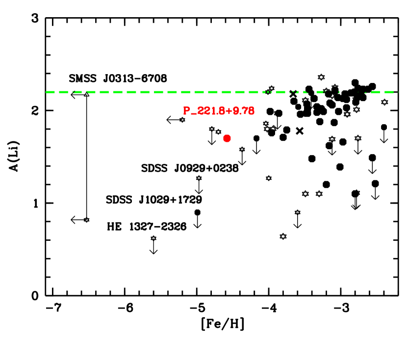
Figure 7: Lithium abundances as a function of [Fe/H] for unevolved stars. The filled black symbols are to carbon-normal stars and the open star-symbols are low carbon band CEMP stars, as defined in Bonifacio et al. (2018a). The literature values of lithium and carbon have been taken from: (Norris et al., 1997; Lucatello et al., 2003; Ivans et al., 2005; Frebel, Johnson & Bromm, 2007; Frebel et al., 2008; Thompson et al., 2008; Aoki et al., 2008; Sbordone et al., 2010; Caffau et al., 2012; Carollo et al., 2012; Masseron et al., 2012; Aoki et al., 2013; Ito et al., 2013; Carollo et al., 2013; Spite et al., 2013; Roederer et al., 2014; Aoki, 2015; Bonifacio et al., 2012; Li et al., 2015; Hansen et al., 2014; Caffau et al., 2016; Placco et al., 2016; Matsuno et al., 2017; Bonifacio et al., 2018a). The two components of the binary system CS 22876-32 (González Hernández et al., 2008) are shown as black crosses. All the stars in this plot are unevolved, except for SMSS J031300.36-670839.3, which is a giant for which we take A(Li) and the upper limit on Fe from Nordlander et al. (2017). The triangle, connected by a line to the measured point of SMSS J031300.36-670839.3 corresponds to the value corrected for dilution as computed by Mucciarelli, Salaris & Bonifacio (2012) for giant stars below the RGB bump. The green dashed line is the level of the Spite plateau as determined by Sbordone et al. (2010).

Bonifacio et al. (2018a) noted that, among stars with [Fe/H]$<-3.5$ and $T\rm_{eff}$ less than 6000 K, Li is always depleted, suggesting that the edge for Li depletion becomes hotter for the more metal-poor stars. Pristine_221.8781+9.7844 follows this general behaviour.

5.4 Other abundance constraints

For several other elements where no detection could be established, we derived an upper limit. In the UVES spectrum, some Al lines are present but are very weak, and we derived from them an upper limit of A(Al) $\leqslant$ 1.6. The Sr ii line at 4077.7 $\AA$ can be seen, but looks distinctly non-Gaussian in shape, which is why we also treat this line as an upper limit of A(Sr) $\leqslant-1.5$.

5.5 Non-LTE and 3D effects

With the exception of the Lithium abundance, all abundances derived in Section 5.3 do not take any non-LTE or 3D corrections into account. However, we note that SDSS J102915+172927, which has very similar stellar parameters as Pristine_221.8781+9.7844 (see Section 6) has been analysed using 3D and non-LTE for many elements, as described in Caffau et al. (2012). This, however, does not predict the combined 3D non-LTE correction strength as the two effects influence each other and a full 3D non-LTE correction cannot be achieved by adding a separate 3D correction and additionally a non-LTE correction.

A complete 3D, non-LTE correction to the abundances is also beyond the scope of this paper but, because of these striking similarities between the two stars, we refer the reader to the 3D and non-LTE corrections derived for SDSS J102915+172927 as indicative of the magnitude of the corrections expected for the elements presented here. For SDSS J102915+172927, the 1D non-LTE correction for [Fe/H] is +0.13, while the 3D LTE correction is $-$0.27. Most significantly, the 3D LTE study impacts the [C/H] abundance ratio (see also Section 5.2), which is corrected by $-$0.7 dex. No non-LTE calculations are available for this abundance derived from molecular CH. The 1D non-LTE calculations that are available for other elements in SDSS J102915+172927 show the largest correction for Si ($-0.34$ dex). The non-LTE corrections for neutral and once ionised Ca tend to go in opposite directions (each by $\sim$0.25 dex) and will make the discrepancy between the two abundances smaller in Pristine_221.8781+9.7844. We further note that the corrections for 1D non-LTE typically increase with decreasing log(g) such that Pristine_221.8781+9.7844 log(g) = 3.5 needs a slightly larger correction than a log(g) = 4.0 star like SDSS J102915+172927 (see Table 4 of Caffau et al., 2012), however, the differences in the corrections are not large enough to cover the difference in the [$\alpha$/Fe] pattern we observe for the two stars. Overall, we can conclude that 3D and non-LTE corrections will improve our detailed picture of the abundances in Pristine_221.8781+9.7844  but that the global properties of the star will not be significantly affected.

6 Comparison to the most metal-poor stars known

Figure 8: Comparison of Pristine_221.8781+9.7844 with the spectrum of SDSS J102915+172927. The spectrum of SDSS J102915+172927 is also taken with the same UVES setup and can thus be directly compared. From top left to bottom right the panels are centred on the Ca II K line, the Ca II H line, the Mg triplet, and a region with many Fe lines respectively. In the top left panel we see both the Ca II K absorption feature from the star itself as well as an interstellar component. Because the stars have different radial velocities and are shifted here to their stellar spectral rest wavelength, the interstellar components appear at different wavelengths in this figure. A great advantage of the high-resolution spectrum is that it resolves these two features, so that interstellar Ca absorption is not confused with stellar Ca.

Figure 9: The results of our abundance analysis for Pristine_221.8781+9.7844  from 1D LTE analysis (large red asterisk) and through face-value applications of the 3D corrections on carbon and iron from Caffau et al. (2012) (larger red asterisk) compared to a literature sample as collected by Aguado et al. (2017), including samples from Frebel et al. (2005), Sivarani et al. (2006), Frebel et al. (2006), Yong et al. (2013), Allende Prieto et al. (2015), and Aguado et al. (2016). The values shown for the 11 stars below [Fe/H]$<-4.5$ are plotted separately and their values are taken from Collet, Asplund & Trampedach (2006); Frebel et al. (2008); Caffau et al. (2011a); Norris et al. (2012); Bessell et al. (2015); Hansen et al. (2015); Frebel et al. (2015); Bonifacio et al. (2015); Caffau et al. (2016); Nordlander et al. (2017); Bonifacio et al. (2018a); Aguado et al. (2018a); and Aguado et al. (2018b). All data shown as blue smaller circles are derived using 1D-LTE. Where possible we also show 3D-LTE values, these are shown as larger circles and connected to the 1D-LTE values for the same star by a dotted line. For two stars, this line is vertical, as only 3D corrections for A(C) are available and not for [Fe/H]. The most iron-poor star, SMSS J031300.36-670839.3, has an analysis in 3D-non-LTE for its upper limit of [Fe/H] by Nordlander et al. (2017) and this is the value shown here. The most metal-poor star in the literature, SDSS J102915+172927, is labelled by a blue filled circle as well as a small white triangle, HE 0557-4840 is highlighted similarly by a small white square. The horizontal lines give the average A(C) for the various carbon-enhanced star groups as defined by Spite et al. (2013).

We note that most metal-poor star known, SDSS J102915+172927, as discovered by Caffau et al. (2011a), has similar stellar parameters to Pristine_221.8781+9.7844, including a very similar colour, ($g-z$) = 0.592. Caffau et al. (2012) derive a $T\rm_{eff}$ of 5811 $\pm$ 150 K, a microturbulent velocity of 1.5 $\mathrm{km\,s^{-1}}$, and a log(g) of 4.0 $\pm 0.5$ dex (they favoured a larger log(g) rather than a smaller log(g) from the Ca ionisation balance and indeed Gaia DR2 confirms that the star is still on the main-sequence from its larger parallax of 0.734 $\pm$ 0.078, see also Bonifacio et al. 2018c). The 1D LTE [Fe/H] = $-4.73\pm 0.13$ is also consistent with the analysis of Pristine_221.8781+9.7844. The $\alpha$-element abundances in SDSS J102915+172927 are significantly smaller, though. In Figure 8, we compare the spectrum that we obtained for Pristine_221.8781+9.7844 directly with SDSS J102915+172927, the most metal-poor star known as studied by Caffau et al. (2011a) using exactly the same UVES setup and spectral reduction techniques. Several items stand out when comparing these two spectra. First of all, we see that the Ca II lines are quite comparable in strength (note that in both spectra one can also see features of interstellar Ca that are resolved at this resolution, and that redwards of Ca II H, we see the strong H$\epsilon$ feature). The Mg triplet is stronger in Pristine_221.8781+9.7844, but the Fe lines are comparable in strength, confirming again an elevation in the $\alpha$-elements in Pristine_221.8781+9.7844 compared to SDSS J102915+172927.

Figure 9 presents the results for our star in 1D LTE and, tentatively, in 3D LTE by straightforwardly applying the corrections of Caffau et al. (2012) for SDSS J102915+172927 in A(C)–[Fe/H] space. Overplotted are a literature sample of extremely metal-poor stars as collected by Aguado et al. (2017) based on samples from Frebel et al. (2005), Sivarani et al. (2006), Frebel et al. (2006), Yong et al. (2013), Allende Prieto et al. (2015), and Aguado et al. (2016). The 12 stars shown in Figure 9 below [Fe/H]$<-4.5$ use the measurements from Collet, Asplund & Trampedach (2006); Frebel et al. (2008); Caffau et al. (2011a); Norris et al. (2012); Bessell et al. (2015); Hansen et al. (2015); Frebel et al. (2015); Bonifacio et al. (2015); Caffau et al. (2016); Nordlander et al. (2017); Bonifacio et al. (2018a); Aguado et al. (2018a, b). Where available, we show both the 1D LTE and 3D LTE measurements as connected symbols of different sizes. For SMSS J031300.36-670839.3, the value of [Fe/H] $<-7.0$ corresponds to the analysis from combined 3D-non-LTE from Nordlander et al. (2017), for all other stars and abundances 3D LTE analyses are shown.

Figure 10: A comparison of the 1D LTE abundances for Pristine_221.8781+9.7844 (red triangles, data from this work), SDSS J102915+172927 (blue diamonds, data from Caffau et al., 2012), and HE 0557-4840 (grey asterisks, data from Norris et al., 2007, 2012), overplotted by a shifted solar abundance scale with [Fe/H] = $-$4.66 following the solar abundances from Lodders, Palme & Gail (2009) with C and Fe solar abundances taken from Caffau et al. (2011b).

It is clear that Pristine_221.8781+9.7844 has a very low metal abundance — not just in [Fe/H], but also in the combination of [Fe/H] and A(C). Because of the relatively large contribution of carbon to the total budget of metals in most stars, this means it is among the most metal-poor stars known. Our upper limit for A(C) in 1D LTE places this star just above the [C/Fe] = +1 line. If we simply adopt the same 3D corrections for carbon and iron from Caffau et al. (2012) – justified by the similarity of both stars in abundance space and stellar parameters – the upper limit falls instead on the [C/Fe] = +1 dividing line between carbon-enhanced and carbon-normal stars according to the definition of Beers & Christlieb (2005). This would suggest the star is carbon-normal, or even carbon-depleted, according to this definition (although in some other studies a level of +0.7 instead of +1.0 is adopted for carbon-rich stars; see, e.g., Aoki et al., 2007). In any case, Pristine_221.8781+9.7844 falls clearly at the low end of the lowest carbon band as defined by Spite et al. (2013) (and represented by the horizontal lines in Figure 9). Similarly, in the classification of Yoon et al. (2016), it would fall in their Group II (if it would be classified as a carbon-enhanced star).

Besides its similarity to SDSS J102915+172927, Pristine_221.8781+9.7844  is quite close in A(C)–[Fe/H] space to HE 0557-4840 (Norris et al., 2007, 2012). This star has $T\rm_{eff}$ = 4900 K and log(g) = 2.2 and is situated on the red giant branch and thus not in the same evolutionary state as either Pristine_221.8781+9.7844  or SDSS J102915+172927. It clearly belongs to the ultra metal-poor class of stars with [Fe/H] = $-4.8$ and, above all, it has only a moderate enhancement in the C, N, and O abundances with [C/Fe]= +1.1, [N/Fe] $<$ +0.1, and [O/Fe] = +1.4 (all corrected for 3D effects, see Norris et al., 2012). These stars have clearly a lower carbon abundance than the majority of the stars in this range of metallicity. In Figure 10, the 1D LTE abundance patterns for Pristine_221.8781+9.7844  SDSS J102915+172927, and HE 0557-4840 are directly compared. It is clear that Pristine_221.8781+9.7844  and to a lesser extent HE 0557-4840, are a bit more enhanced in $\alpha$-elements than SDSS J102915+172927, but overall the abundance patterns are quite similar for the elements measured in multiple stars.

7 Conclusions

In this paper, we present the discovery of the ultra metal-poor sub-giant star, Pristine_221.8781+9.7844, from Ca H&K narrow-band photometry. We also present an analysis of follow-up medium- and high-resolution spectra using a variety of analysis methods. Pristine_221.8781+9.7844  is found to be similar to the most metal-poor star known (SDSS J102915+172927, Caffau et al., 2011a) in terms of stellar parameters, as well as [Fe/H] in standard 1D LTE analysis. A direct comparison of the standard 1D LTE abundances and the spectra (see Figure 8) reveals, however, that Pristine_221.8781+9.7844  has an [$\alpha$/Fe] ratio of 0.3–0.4 dex, significantly larger than that of SDSS J102915+172927. This is most clearly evident in a stronger Mg triplet feature. Like SDSS J102915+172927, it has no detectable CH features. This leaves open the possibility that this star is carbon-normal, or even carbon-depleted, which would be an anomaly at this extremely low [Fe/H] level. Pristine_221.8781+9.7844  also bears a striking resemblance in abundance pattern to HE 0557-4840 (Norris et al., 2007, 2012). Lacking any clear measurement of C, N, and O features in the spectrum of Pristine_221.8781+9.7844 and SDSS J102915+172927, it would be premature to argue which star is the most metal-deficient overall, and this is perhaps not the most pressing question at this time. Rather, it is clear that these objects belong to a class of rare, ultra metal-deficient stars that can provide important constraints on cooling and formation of long-lived stars in the low metallicity environment of the early Galaxy.

Appendix A Line list

Table 5 presents the used line list for Fe lines; Table 6 lists all lines used in the analyses of other elements. Measurement uncertainties for the equivalent width methods are not presented, as the total uncertainties are instead dominated by the continuum placement. This is the main source of the systematic discrepancy between the two equivalent width methods (methods 3 and 4). Despite these discrepancies in measurements, the resulting abundance determinations are compatible within their uncertainties (as illustrated in Section 5, with the exception of Ca and Ti that show 0.1 dex difference).

Wavelength	Ion	$\chi$	log(gf)	used	used	EW (m$\AA$)	EW (m$\AA$)
($\AA$)				method1	method2	method3	method4
5328.531	Fe i	1.56	$-$1.85	X	–	–	–
5269.537	Fe i	0.86	$-$1.33	X	X	–	14
4415.122	Fe i	1.61	$-$0.62	X	–	10	–
4404.750	Fe i	1.56	$-$0.15	X	X	19	22
4383.545	Fe i	1.48	0.21	X	X	32	38
4325.762	Fe i	1.61	0.01	X	X	13	15
4307.910	Fe i	1.56	$-$0.07	–	X	–	15
4294.140	Fe i	1.49	$-$1.11	–	–	–	6
4271.761	Fe i	1.48	$-$0.17	X	X	18	22
4260.474	Fe i	2.40	0.08	X	–	11	10
4202.029	Fe i	1.48	$-$0.69	X	–	–	–
4143.868	Fe i	1.56	$-$0.51	X	X	–	7
4071.738	Fe i	1.61	$-$0.01	X	X	19	23
4067.978	Fe i	3.21	$-$0.53	X	–	–	–
4063.594	Fe i	1.56	0.06	X	X	16	23
4045.812	Fe i	1.48	0.28	X	–	30	29
4005.242	Fe i	1.56	$-$0.58	X	–	–	12
3930.297	Fe i	0.09	$-$1.49	–	X	–	29
3927.921	Fe i	0.11	$-$1.52	–	X	–	29
3922.912	Fe i	0.05	$-$1.63	X	X	17	19
3920.258	Fe i	0.12	$-$1.73	X	X	10	15
3906.479	Fe i	0.11	$-$2.21	–	X	–	–
3902.945	Fe i	1.56	$-$0.44	–	–	11	–
3899.707	Fe i	0.09	$-$1.51	X	X	23	33
3895.656	Fe i	0.11	$-$1.67	X	X	23	24
3887.048	Fe i	0.91	$-$1.09	X	–	–	–
3886.282	Fe i	0.05	$-$1.05	X	X	45	52
3878.573	Fe i	0.09	$-$1.38	–	X	22	27
3878.018	Fe i	0.96	$-$0.90	–	X	17	–
3865.523	Fe i	4.14	$-$0.93	X	X	–	–
3859.912	Fe i	0.00	$-$0.70	X	–	56	62
3859.213	Fe i	2.40	$-$0.68	–	X	–	–
3856.372	Fe i	0.05	$-$1.28	X	X	35	36
3849.967	Fe i	1.01	$-$0.86	X	–	16	–
3841.048	Fe i	1. 61	$-$0.04	X	–	–	–
3840.438	Fe i	0.99	$-$0.50	X	–	–	–
3834.222	Fe i	0.96	$-$0.27	–	X	–	–
3827.823	Fe i	1.56	0.09	X	–	15	–
3825.881	Fe i	0.91	$-$0.02	X	X	33	43
3824.444	Fe i	0.00	$-$1.34	X	X	30	36
3820.425	Fe i	0.86	0.16	X	X	48	59
3815.840	Fe i	1.48	0.24	X	–	30	35
3812.964	Fe i	0.96	$-$1.05	–	X	–	–
3767.192	Fe i	1.01	$-$0.38	X	X	–	–
3763.789	Fe i	0.99	$-$0.22	X	X	28	35
3758.233	Fe i	0.96	$-$0.01	–	X	37	38
3745.561	Fe i	0.09	$-$0.77	–	X	–	50
3745.899	Fe i	0.12	$-$1.34	–	–	–	28
3748.262	Fe i	0.11	$-$1.01	–	–	–	41
3737.131	Fe i	0.05	$-$0.57	–	X	–	56
3734.884	Fe i	0.86	0.33	–	X		–
3727.619	Fe i	0.96	$-$0.61	X	–	17	–
3722.563	Fe i	0.09	$-$1.28	–	X	–	–
3719.935	Fe i	0.00	$-$0.42	–	–	73	79
3705.566	Fe i	0.05	$-$1.32	–	–	–	32
3709.246	Fe i	0.91	$-$0.62	–	–	–	29

Table 5: Line list of Fe lines used in the analysis.

Wavelength	Ion	$\chi$	log(gf)	used	used	EW (m$\AA$)	EW (m$\AA$)
($\AA$)				method1	method2	method3	method4
5895.924	Na i	0.00	$-$0.19	X	–	–	13
5889.970	Na i	0.00	0.11	X	–	25	21
5183.604	Mg i	2.72	$-$0.16	X	X	39	37
5172.700	Mg i	2.71	$-$0.38	X	X	30	30
5167.31	Mg i	2.71	$-$1.03	X	X	–	12
3838.292	Mg i	2.72	0.42	X	–	–	64
3832.304	Mg i	2.71	0.150	X	–	49	50
3829.355	Mg i	2.71	$-$0.23	X	–	24	31
3905.523	Si i	1.91	$-$1.09	X	X	23	22
4226.728	Ca i	0.00	0.24	X	X	32	37
3736.902	Ca ii	3.15	$-$0.15	X	–	–	–
3933.663	Ca ii	0.00	0.13	X	–	–	–
3968.470	Ca ii	0.00	$-$0.17	X	–	–	–
3759.292	Ti ii	0.61	0.28	X	–	32	38
3761.321	Ti ii	0.57	0.18	X	X	28	35
4077.710	Sr ii	0.00	0.17	X	–	12	7

Table 6: Line list of elements other than Fe used in the analysis.

References

- Aguado et al. (2016) Aguado D. S., Allende Prieto C., González Hernández J. I., Carrera R., Rebolo R., Shetrone M., Lambert D. L., Fernández-Alvar E., 2016, A&A, 593, A10
- Aguado et al. (2018b) Aguado D. S., Allende Prieto C., González Hernández J. I., Rebolo R., 2018b, ApJ, 854, L34
- Aguado et al. (2017) Aguado D. S., González Hernández J. I., Allende Prieto C., Rebolo R., 2017, A&A, 605, A40
- Aguado et al. (2018a) —, 2018a, ApJ, 852, L20
- Albareti et al. (2017) Albareti F. D. et al., 2017, ApJS, 233, 25
- Allende Prieto et al. (2006) Allende Prieto C., Beers T. C., Wilhelm R., Newberg H. J., Rockosi C. M., Yanny B., Lee Y. S., 2006, ApJ, 636, 804
- Allende Prieto et al. (2015) Allende Prieto C. et al., 2015, A&A, 579, A98
- Alvarez & Plez (1998) Alvarez R., Plez B., 1998, A&A, 330, 1109
- Andrae et al. (2018) Andrae R. et al., 2018, ArXiv e-prints
- Anthony-Twarog et al. (2000) Anthony-Twarog B. J., Sarajedini A., Twarog B. A., Beers T. C., 2000, AJ, 119, 2882
- Anthony-Twarog et al. (1991) Anthony-Twarog B. J., Twarog B. A., Laird J. B., Payne D., 1991, AJ, 101, 1902
- Aoki (2015) Aoki W., 2015, ApJ, 811, 64
- Aoki et al. (2009) Aoki W., Barklem P. S., Beers T. C., Christlieb N., Inoue S., García Pérez A. E., Norris J. E., Carollo D., 2009, ApJ, 698, 1803
- Aoki et al. (2007) Aoki W., Beers T. C., Christlieb N., Norris J. E., Ryan S. G., Tsangarides S., 2007, ApJ, 655, 492
- Aoki et al. (2013) Aoki W. et al., 2013, AJ, 145, 13
- Aoki et al. (2008) —, 2008, ApJ, 678, 1351
- Bailer-Jones et al. (2013) Bailer-Jones C. A. L. et al., 2013, A&A, 559, A74
- Barklem, Piskunov & O’Mara (2000a) Barklem P. S., Piskunov N., O’Mara B. J., 2000a, A&A, 355, L5
- Barklem, Piskunov & O’Mara (2000b) —, 2000b, A&A, 363, 1091
- Beers & Christlieb (2005) Beers T. C., Christlieb N., 2005, ARA&A, 43, 531
- Beers, Preston & Shectman (1985) Beers T. C., Preston G. W., Shectman S. A., 1985, AJ, 90, 2089
- Bessell et al. (2015) Bessell M. S. et al., 2015, ApJ, 806, L16
- Bonifacio et al. (2018b) Bonifacio P. et al., 2018b, A&A, 611, A68
- Bonifacio et al. (2015) —, 2015, A&A, 579, A28
- Bonifacio et al. (2018c) —, 2018c, ArXiv e-prints
- Bonifacio et al. (2018a) —, 2018a, ArXiv e-prints
- Bonifacio et al. (2007) —, 2007, A&A, 462, 851
- Bonifacio et al. (2012) Bonifacio P., Sbordone L., Caffau E., Ludwig H.-G., Spite M., González Hernández J. I., Behara N. T., 2012, A&A, 542, A87
- Bromm (2013) Bromm V., 2013, Reports on Progress in Physics, 76, 112901
- Caffau et al. (2011a) Caffau E. et al., 2011a, Nature, 477, 67
- Caffau et al. (2012) —, 2012, A&A, 542, A51
- Caffau et al. (2016) —, 2016, A&A, 595, L6
- Caffau et al. (2017) —, 2017, Astronomische Nachrichten, 338, 686
- Caffau et al. (2010) Caffau E., Ludwig H.-G., Bonifacio P., Faraggiana R., Steffen M., Freytag B., Kamp I., Ayres T. R., 2010, A&A, 514, A92
- Caffau et al. (2011b) Caffau E., Ludwig H.-G., Steffen M., Freytag B., Bonifacio P., 2011b, Sol. Phys., 268, 255
- Carollo et al. (2012) Carollo D. et al., 2012, ApJ, 744, 195
- Carollo et al. (2013) Carollo D., Martell S. L., Beers T. C., Freeman K. C., 2013, ApJ, 769, 87
- Casagrande et al. (2010) Casagrande L., Ramírez I., Meléndez J., Bessell M., Asplund M., 2010, A&A, 512, A54
- Castelli (2005) Castelli F., 2005, Memorie della Societa Astronomica Italiana Supplementi, 8, 25
- Castelli & Kurucz (2004) Castelli F., Kurucz R. L., 2004, ArXiv Astrophysics e-prints
- Chiaki, Tominaga & Nozawa (2017) Chiaki G., Tominaga N., Nozawa T., 2017, MNRAS, 472, L115
- Choi et al. (2016) Choi J., Dotter A., Conroy C., Cantiello M., Paxton B., Johnson B. D., 2016, ApJ, 823, 102
- Christlieb, Wisotzki & Graßhoff (2002) Christlieb N., Wisotzki L., Graßhoff G., 2002, A&A, 391, 397
- Collet, Asplund & Trampedach (2006) Collet R., Asplund M., Trampedach R., 2006, ApJ, 644, L121
- Dekker et al. (2000) Dekker H., D’Odorico S., Kaufer A., Delabre B., Kotzlowski H., 2000, in Proc. SPIE, Vol. 4008, Optical and IR Telescope Instrumentation and Detectors, Iye M., Moorwood A. F., eds., pp. 534–545
- Den Hartog et al. (2014) Den Hartog E. A., Ruffoni M. P., Lawler J. E., Pickering J. C., Lind K., Brewer N. R., 2014, ApJS, 215, 23
- Dotter (2016) Dotter A., 2016, ApJS, 222, 8
- Frebel et al. (2005) Frebel A. et al., 2005, Nature, 434, 871
- Frebel et al. (2015) Frebel A., Chiti A., Ji A. P., Jacobson H. R., Placco V. M., 2015, ApJ, 810, L27
- Frebel et al. (2006) Frebel A. et al., 2006, ApJ, 652, 1585
- Frebel et al. (2008) Frebel A., Collet R., Eriksson K., Christlieb N., Aoki W., 2008, ApJ, 684, 588
- Frebel, Johnson & Bromm (2007) Frebel A., Johnson J. L., Bromm V., 2007, MNRAS, 380, L40
- Gaia Collaboration et al. (2018) Gaia Collaboration, Brown A. G. A., Vallenari A., Prusti T., de Bruijne J. H. J., Babusiaux C., Bailer-Jones C. A. L., 2018, ArXiv e-prints
- González Hernández & Bonifacio (2009) González Hernández J. I., Bonifacio P., 2009, A&A, 497, 497
- González Hernández et al. (2008) González Hernández J. I. et al., 2008, A&A, 480, 233
- Greif (2015) Greif T. H., 2015, Computational Astrophysics and Cosmology, 2, 3
- Guiglion et al. (2016) Guiglion G., de Laverny P., Recio-Blanco A., Worley C. C., De Pascale M., Masseron T., Prantzos N., Mikolaitis Š., 2016, A&A, 595, A18
- Gustafsson et al. (2008) Gustafsson B., Edvardsson B., Eriksson K., Jørgensen U. G., Nordlund Å., Plez B., 2008, A&A, 486, 951
- Hansen et al. (2015) Hansen T. et al., 2015, ApJ, 807, 173
- Hansen et al. (2014) —, 2014, ApJ, 787, 162
- Henden et al. (2012) Henden A. A., Levine S. E., Terrell D., Smith T. C., Welch D., 2012, Journal of the American Association of Variable Star Observers (JAAVSO), 40, 430
- Howes et al. (2015) Howes L. M. et al., 2015, Nature, 527, 484
- Ito et al. (2013) Ito H., Aoki W., Beers T. C., Tominaga N., Honda S., Carollo D., 2013, ApJ, 773, 33
- Ivans et al. (2005) Ivans I. I., Sneden C., Gallino R., Cowan J. J., Preston G. W., 2005, ApJ, 627, L145
- Ivezic et al. (2014) Ivezic Z., Connolly A. J., VanderPlas J. T., Gray A., 2014, Statistics, Data Mining, and Machine Learning in Astronomy: A Practical Python Guide for the Analysis of Survey Data. Princeton University Press, Princeton, NJ, USA
- Jorden (1990) Jorden P. R., 1990, in Proc. SPIE, Vol. 1235, Instrumentation in Astronomy VII, Crawford D. L., ed., pp. 790–798
- Jordi, Grebel & Ammon (2006) Jordi K., Grebel E. K., Ammon K., 2006, A&A, 460, 339
- Kafle et al. (2014) Kafle P. R., Sharma S., Lewis G. F., Bland-Hawthorn J., 2014, ApJ, 794, 59
- Keller et al. (2014) Keller S. C. et al., 2014, Nature, 506, 463
- Keller et al. (2007) —, 2007, Publ. Astron. Soc. Australia, 24, 1
- Koch et al. (2016) Koch A., McWilliam A., Preston G. W., Thompson I. B., 2016, A&A, 587, A124
- Koesterke, Allende Prieto & Lambert (2008) Koesterke L., Allende Prieto C., Lambert D. L., 2008, ApJ, 680, 764
- Kurucz & Bell (1995) Kurucz R., Bell B., 1995, Atomic Line Data (R.L. Kurucz and B. Bell) Kurucz CD-ROM No. 23. Cambridge, Mass.: Smithsonian Astrophysical Observatory, 1995., 23
- Kurucz (2005) Kurucz R. L., 2005, Memorie della Societa Astronomica Italiana Supplementi, 8, 14
- Lawrence et al. (2012) Lawrence A. et al., 2012, VizieR Online Data Catalog, 2314
- Li et al. (2015) Li H., Aoki W., Zhao G., Honda S., Christlieb N., Suda T., 2015, PASJ, 67, 84
- Lodders, Palme & Gail (2009) Lodders K., Palme H., Gail H.-P., 2009, Landolt Börnstein
- Lucatello et al. (2003) Lucatello S., Gratton R., Cohen J. G., Beers T. C., Christlieb N., Carretta E., Ramírez S., 2003, AJ, 125, 875
- Ludwig et al. (2008) Ludwig H.-G., Bonifacio P., Caffau E., Behara N. T., González Hernández J. I., Sbordone L., 2008, Physica Scripta Volume T, 133, 014037
- Masseron et al. (2012) Masseron T., Johnson J. A., Lucatello S., Karakas A., Plez B., Beers T. C., Christlieb N., 2012, ApJ, 751, 14
- Matsuno et al. (2017) Matsuno T., Aoki W., Beers T. C., Lee Y. S., Honda S., 2017, AJ, 154, 52
- Mészáros et al. (2012) Mészáros S. et al., 2012, AJ, 144, 120
- Mucciarelli (2013) Mucciarelli A., 2013, ArXiv e-prints
- Mucciarelli et al. (2013b) Mucciarelli A., Pancino E., Lovisi L., Ferraro F. R., Lapenna E., 2013b, GALA: Stellar atmospheric parameters and chemical abundances. Astrophysics Source Code Library
- Mucciarelli, Salaris & Bonifacio (2012) Mucciarelli A., Salaris M., Bonifacio P., 2012, MNRAS, 419, 2195
- Murphy et al. (2009) Murphy S., Keller S., Schmidt B., Tisserand P., Bessell M., Francis P., Costa G. D., 2009, in Astronomical Society of the Pacific Conference Series, Vol. 404, The Eighth Pacific Rim Conference on Stellar Astrophysics: A Tribute to Kam-Ching Leung, Soonthornthum B., Komonjinda S., Cheng K. S., Leung K. C., eds., p. 356
- Nordlander et al. (2017) Nordlander T., Amarsi A. M., Lind K., Asplund M., Barklem P. S., Casey A. R., Collet R., Leenaarts J., 2017, A&A, 597, A6
- Norris et al. (2012) Norris J. E., Christlieb N., Bessell M. S., Asplund M., Eriksson K., Korn A. J., 2012, ApJ, 753, 150
- Norris et al. (2007) Norris J. E., Christlieb N., Korn A. J., Eriksson K., Bessell M. S., Beers T. C., Wisotzki L., Reimers D., 2007, ApJ, 670, 774
- Norris et al. (1997) Norris J. E., Ryan S. G., Beers T. C., Deliyannis C. P., 1997, ApJ, 485, 370
- Norris et al. (2013) Norris J. E. et al., 2013, ApJ, 762, 28
- O’Brian et al. (1991) O’Brian T. R., Wickliffe M. E., Lawler J. E., Whaling W., Brault J. W., 1991, Journal of the Optical Society of America B Optical Physics, 8, 1185
- Omukai, Schneider & Haiman (2008) Omukai K., Schneider R., Haiman Z., 2008, ApJ, 686, 801
- Paxton et al. (2011) Paxton B., Bildsten L., Dotter A., Herwig F., Lesaffre P., Timmes F., 2011, ApJS, 192, 3
- Placco et al. (2016) Placco V. M., Beers T. C., Reggiani H., Meléndez J., 2016, ApJ, 829, L24
- Plez (2008) Plez B., 2008, Physica Scripta Volume T, 133, 014003
- Plez & Lambert (2002) Plez B., Lambert D. L., 2002, A&A, 386, 1009
- Roederer et al. (2014) Roederer I. U., Preston G. W., Thompson I. B., Shectman S. A., Sneden C., Burley G. S., Kelson D. D., 2014, AJ, 147, 136
- Sbordone (2005) Sbordone L., 2005, Memorie della Societa Astronomica Italiana Supplementi, 8, 61
- Sbordone et al. (2010) Sbordone L. et al., 2010, A&A, 522, A26
- Sbordone et al. (2004) Sbordone L., Bonifacio P., Castelli F., Kurucz R. L., 2004, Memorie della Societa Astronomica Italiana Supplementi, 5, 93
- Sbordone et al. (2014) Sbordone L., Caffau E., Bonifacio P., Duffau S., 2014, A&A, 564, A109
- Schlegel, Finkbeiner & Davis (1998) Schlegel D. J., Finkbeiner D. P., Davis M., 1998, ApJ, 500, 525
- Schneider et al. (2012b) Schneider R., Omukai K., Bianchi S., Valiante R., 2012b, MNRAS, 419, 1566
- Schneider et al. (2012a) Schneider R., Omukai K., Limongi M., Ferrara A., Salvaterra R., Chieffi A., Bianchi S., 2012a, MNRAS, 423, L60
- Sivarani et al. (2006) Sivarani T. et al., 2006, A&A, 459, 125
- Skrutskie et al. (2006) Skrutskie M. F. et al., 2006, AJ, 131, 1163
- Smiljanic et al. (2014) Smiljanic R. et al., 2014, A&A, 570, A122
- Sneden (1973) Sneden C., 1973, ApJ, 184, 839
- Spite & Spite (1982b) Spite F., Spite M., 1982b, A&A, 115, 357
- Spite et al. (2013) Spite M., Caffau E., Bonifacio P., Spite F., Ludwig H.-G., Plez B., Christlieb N., 2013, A&A, 552, A107
- Spite & Spite (1982a) Spite M., Spite F., 1982a, Nature, 297, 483
- Starkenburg et al. (2017) Starkenburg E. et al., 2017, MNRAS, 471, 2587
- Stetson & Pancino (2008) Stetson P. B., Pancino E., 2008, PASP, 120, 1332
- Thompson et al. (2008) Thompson I. B. et al., 2008, ApJ, 677, 556
- Wood et al. (2013) Wood M. P., Lawler J. E., Sneden C., Cowan J. J., 2013, ApJS, 208, 27
- Yong et al. (2013) Yong D. et al., 2013, ApJ, 762, 27
- Yoon et al. (2016) Yoon J. et al., 2016, ApJ, 833, 20
- Youakim et al. (2017) Youakim K. et al., 2017, MNRAS, 472, 2963