The Halo’s Ancient Metal-Rich Progenitor Revealed with BHB Stars

Abstract

Using the data from the Sloan Digital Sky Survey and the Gaia satellite, we assemble a pure sample of $\sim$3000 Blue Horizontal Branch (BHB) stars with 7-D information, including positions, velocities and metallicities. We demonstrate that, as traced with BHBs, the Milky Way’s stellar halo is largely unmixed and can not be well represented with a conventional Gaussian velocity distribution. A single-component model fails because the inner portions of the halo are swamped with metal-rich tidal debris from an ancient, head-on collision, known as the “Gaia Sausage”. Motivated by the data, we build a flexible mixture model which allows us to track the evolution of the halo make-up across a wide range of radii. It is built from two components, one representing the radially anisotropic Sausage stars with their lobed velocity distribution, the other representing a more metal-poor and more isotropic component built up from minor mergers. We show that inside 25 kpc the “Sausage" contributes at least 50% of the Galactic halo. The fraction of “Sausage" stars diminishes sharply beyond 30 kpc, which is the long-established break radius of the classical stellar halo.

1 Introduction

Understanding the dynamics of the Milky Way’s stellar halo is not only key to understanding the formation mechanism of the halo itself (Eggen et al., 1962; Searle & Zinn, 1978), but also for constraining the mass distribution of the Milky Way (Xue et al., 2008; Gnedin et al., 2010; Deason et al., 2012), the history of structures accreted in the stellar halo (Frenk & White, 1980; Johnston et al., 2008; Belokurov et al., 2018) and hence the cold dark matter (CDM) paradigm of hierarchical structure formation. Due to the wide range of applications for detailed measurements of the velocity ellipsoid of the stellar halo, much effort has been made in understanding its kinematic structure (Frenk & White, 1980; Bekki & Chiba, 2001; Sirko et al., 2004; Battaglia et al., 2005; Smith et al., 2009a; Kafle et al., 2012, 2013). This characterization has sometimes proceeded by using the full phase space distribution function (Williams & Evans, 2015; Das & Binney, 2016). More commonly, just the first and second moments of the velocity distribution are measured (Chiba & Yoshii, 1998; Xue et al., 2008; Bond et al., 2010; Bowden et al., 2016; Cunningham et al., 2016).

These kinematic properties of the stellar halo can be compactly described by the anisotropy parameter $\beta$ defined as:

$$\beta=1-\frac{\sigma_{\theta}^{2}+\sigma_{\phi}^{2}}{2\sigma_{r}^{2}}$$ (1)

where $\sigma_{r}$, $\sigma_{\theta}$ and $\sigma_{\phi}$ are the velocity dispersions referred to Galactocentric spherical polar coordinates ($r,\theta,\phi$). The usefulness of $\beta$ is greatly enhanced if the velocity dispersion tensor is aligned in spherical polar coordinates, as otherwise there are cross-terms which contain additional kinematic information.

Before the release of Gaia data release 2 (DR2), measurements of $\beta$ have been restricted to the nearby inner halo of the Milky Way due to the lack of measurements of the proper motions of stars out to significant distances in the stellar halo (Chiba & Yoshii, 1998; Smith et al., 2009a; Belokurov et al., 2018). Thus, so far, the attempts to gauge the halo anisotropy in the Galactic outskirts have been few and far between (see e.g. Cunningham et al., 2016; Kafle et al., 2017). With the advent of DR2, we now have unprecedented access to the proper motions of stars deep in the stellar halo (Gaia Collaboration et al., 2016, 2018). During the preparation of this manuscript, Bird et al. (2018) measured the velocity dispersion in the stellar halo using a sample of $\sim$8600 K-Giant stars from the Large Sky Area Multi-Object Fibre Spectroscopic Telescope (LAMOST) Data Release 5 (Cui et al., 2012). This study presented the first measurement of the evolution of the velocity ellipsoid in the Milky Way, out to large Galactocentric radii.

With this paper, we aim to supplement the measurement of Bird et al. (2018) in two ways. First, we analyze a complementary data set of Blue Horizontal Branch (BHB) stars from the Sloan Digital Sky Survey’s (SDSS) Data Release 8, thereby using a different tracer sampled from different parts of the sky. Importantly, the BHB distances outperform those of K-giant stars due to a much weaker dependence on age and metallicity. Second, we carry out a more in-depth analysis that imposes strong outlier filtering and takes into account measurement error, deconvolving the observed distribution via fitting of simplified Gaussian mixture models. Additionally, our examination is motivated by the most recent detection of two distinct components in the nearby stellar halo. The inner halo appears to be dominated by stars deposited in an ancient major accretion event. This dramatic head-on collision deposited into the Milky Way stellar debris on highly radial orbits (e.g., Belokurov et al., 2018; Helmi et al., 2018). This gives rise to a characteristic shape in velocity, the “Gaia Sausage,” a.k.a. “Gaia-Enceladus," a.k.a. “Kraken". These mostly metal-rich stars are mixed with a more metal-poor and isotropic halo component built up from a superposition of various minor mergers (Myeong et al., 2018b). A simple and robust prediction arises as to the behavior of the halo velocity ellipsoid with Galactocentric distance. The “Sausage” stars are not expected to travel far beyond their progenitor’s last apocentre, shown to roughly coincide with the break in the stellar halo (Deason et al., 2011; Deason et al., 2013, 2018). This implies that the fractional contribution of this major merger to the Galactic halo varies with distance and is predicted to diminish substantially beyond 20-30 kpc. Therefore, the overall halo’s velocity anisotropy should reflect the change in the debris mixture, from radial to isotropic as a function of distance, or, more specifically from values close to $\beta\sim 1$ within 20-30 kpc to values close to $\beta\sim 0$ beyond 30 kpc.

We begin in Section 2 by describing the data that we have used and how we have filtered it. Next, we describe our methods of analyzing this data in Section 3. In Section 4, we present the results of this analysis in the form of the kinematics inferred from our models. Finally, we discuss the implications of our measurement for the formation history of the Galaxy and conclude in Section 5.

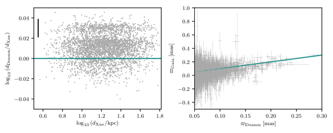
Figure 1: We show a comparison of the different distance measurements available to us, restricting to the stars left after the selections described in section 2, though without removing the Sgr Stream.Left Panels: We show the logarithm of the ratio of the two photometric distance estimates (one given by the Xue catalog and one from the Deason estimate) versus the logarithm of the distances we calculate. We show the logarithm of the distance as this is the space in which the errors are approximately Gaussian for our estimate. In order to avoid cluttering the plot we show the mean error on our estimate as a black bar in the upper left corner of the plot. Right Panels: We show the parallax ($\varpi_{\rm Gaia}$) from the Gaia survey, versus the parallax that would be inferred from our absolute magnitude estimate and errors. The errors on $\varpi_{\rm Deason}$ are 1$\sigma$ errors and are calculated via Monte Carlo propagation. We additionally, restrict to stars with $\varpi_{\rm Deason}>0.05$ as the Gaia parallaxes are only reasonably measured in this region.

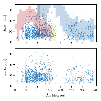
Figure 2: The Removal of Sagittarius (Sgr) Stream Contaminants. Here, we display the data in the plane of Sgr longitude $\tilde{\Lambda}_{\odot}$ versus heliocentric distance $d_{\rm hel}$. The stars in our sample are shown as blue points. Top Panel: The shaded regions on the plot mark the regions in which we would have removed stars if they lay within $\tilde{B}_{\odot}<10^{\circ}$ of the plane of the Sgr Stream. The dark red (blue) region is associated with the leading (trailing) arm, while the yellow region marks additional bins added on to the leading arm. Bottom Panel: The sample that is left after performing the excision of the Sgr Stream.

2 Data

We aim to measure the evolution of the velocity ellipsoid of the Milky Way’s stellar halo as a function of Galactocentric radius. To do this, we need 3D kinematic information for a large sample of stars in the stellar halo. We supplement the proper motion measurements of the Gaia satellite with spectroscopic radial velocity and photometric distance relations for a large sample of Blue Horizontal Branch (BHB) stars.

Our initial sample consists of a catalog of 4,985 BHB stars compiled by Xue et al. (2011). These stars were selected using spectroscopic and photometric information from the SEGUE-1, SEGUE-2, and older SDSS surveys and the data was publicly released as part of SDSS DR8 (Aihara et al., 2011). Xue et al. (2011) used similar spectroscopic and photometric selections as Xue et al. (2008) and Sirko et al. (2004), with some modest relaxations to increase the statistics of the sample. These studies generally aim for high purity samples of BHBs. For this reason, it has generally been accepted that the Xue et al. (2011) sample is of very high purity, and of relatively high completeness when restricted to the survey footprint.

The Xue et al. (2011) catalog includes sky positions, radial velocity measurements with error estimates, and distance estimates to the stars. However, errors on these distance estimates are not provided. In order to have a more robust inference, we extract our own distance and (more importantly) distance error estimates. We do this by cross-matching this sample with SDSS to get the full photometry information and using it along with the distance estimator described in Equation 7 of Deason et al. (2011) to produce our own distance estimates and distance errors, based on Monte Carlo propagation of uncertainty from the photometric uncertainties. Figure 1 shows how our derived distances compare to both the distances that were originally in the catalog as well as Gaia’s parallax measurements after making the sample restrictions described below as well as those in section 2.3. We can see that the distances agree very well.

The Monte Carlo propagation of photometric uncertainty does not include systematic errors in the estimator of Deason et al. (2011) , which should be of comparable order to the errors obtained from the photometric uncertainty. However, both of these errors are small enough that it makes no significant impact on the distribution of errors on Galactocentric velocities. We additionally retrieve metallicity information from cross-matching our sample with the SDSS spectroscopic parameters table from DR8. Including the requirement that the stars have measured metallicities leaves us with 4,879 BHBs.

To make sure we have a cleanest sample of BHBs for the halo kinematics measurement, we make a few additional requirements on the data. We summarize these restrictions here, quoting the number of stars that each selection applies to, though keep in mind that many of the criteria apply to multiple stars:

• The stars have astrometric measurements from the Gaia satellite (removes 22 stars).

• The stars lie within the color box for which the distance estimator from Deason et al. (2011) is valid (this removes 672 stars).

• The astrometric excess noise measured by Gaia is less than 1 mas (removes 26 stars).

• The fractional difference in photometric distance estimate from Deason et al. (2011) and photometric distance estimate from Xue et al. (2011) is less than 10% (removes 197 stars).

• The parallax $\varpi$ and photometric distance $d_{\rm photo}$ satisfy $\varpi-1/d_{\rm photo}<4\sigma_{\varpi}$. This helps us to remove possible Blue Straggler contaminants (see below for more details, this removes 45 stars).

After applying the above selections, we are left with 4,126 BHBs.

2.1 Transformation from Measurement Space

We have the following quantities for each star: Right Ascension and Declination ($\alpha,\delta$), proper motions in Right Ascension and Declination ($\mu_{\alpha},\mu_{\delta}$), errors in those quantities ($\sigma_{\mu_{\alpha}},\sigma_{\mu_{\delta}}$), covariance of the proper motion measurements (${\rm cov}(\mu_{\alpha},\mu_{\delta})$), heliocentric radial velocity ($v_{{\rm hel}}$) and its error ($\sigma_{v_{{\rm hel}}}$), the base 10 logarithmic heliocentric distance to the star ($\log_{10}(d_{\rm hel})$), and its error ($\sigma_{\log_{10}(d_{\rm hel})}$). Here, we assume that all observables (proper motions, radial velocities, and logarithm of distance) are Gaussian distributed. Next, we transform the observables to spherical polar coordinates in the Galactic rest-frame. To account for measurement error, we Monte-Carlo propagate the errors from the data space to our Galactocentric coordinates. We then use these samples to compute the covariance matrix of the 6-D phase space coordinates in the Galactocentric frame for each star. We also assume that the resulting uncertainties on the Galactocentric parameters are still Gaussian. This is not strictly speaking correct, as the transformation does not preserve the Gaussianity of the distributions. However, having checked the kurtosis of the propagated distributions, we find that the effects of any non-Gaussianity are relatively low.

After this transformation, we work with the Galactocentric radius ($r$), the velocity resolved with respect to spherical polar coordinates $(v_{r},v_{\theta},v_{\phi})$, as well as the errors and covariances between all these parameters. Note that in our convention, disc stars have negative angular momentum: that is, $\left\langle v_{\phi,{\rm disk}}\right\rangle\approx-220$ km/s. For the sun’s Galactocentric phase space coordinates, we use the astropy (The Astropy Collaboration et al., 2018) default values with peculiar motion $v_{\odot}=(11.1,-232.24,7.25)$ km/s in Galactocentric Cartesian coordinates, galactocentric distance of $r_{{\rm gc},\odot}=8.3$ kpc, and height above the disk of $z_{\odot}=27$ pc which come from Reid & Brunthaler (2004), Gillessen et al. (2009), Chen et al. (2001), and Schönrich et al. (2010).

2.2 Removal of Sagittarius

In order to make an unbiased measurement of the shape of the velocity ellipsoid, we remove one obvious unrelaxed substructure, i.e. the Sagittarius (Sgr) stream. We use the Sgr coordinate system defined in the Appendix of Belokurov et al. (2014). Restricting to stars within 10^∘ of the plane of the Sgr Stream, we then use the geometry of the stream given by Hernitschek et al. (2017) to remove stars based on their heliocentric distance, rather than relying on sky position alone, thereby avoiding over-cleaning our data. Specifically, at a given Sgr longitude $\tilde{\Lambda}_{\odot}$, we remove any star which satisfies:

$$0<d_{\rm helio}-d_{\rm sgr}<3\sigma_{\rm sgr}+2\left(2\delta_{+}\left(\sigma_{\rm sgr}\right)\right)$$ (2)

or

$$-3\sigma_{\rm sgr}-2\left(2\delta_{-}\left(\sigma_{\rm sgr}\right)\right)<d_{\rm helio}-d_{\rm sgr}<0$$ (3)

where $d_{\rm sgr}$, $\sigma_{\rm sgr}$, $2\delta_{-}\left(\sigma_{\rm sgr}\right)$, and $2\delta_{+}\left(\sigma_{\rm sgr}\right)$ are taken from columns 3,8,11, and 12 (respectively) of tables A4 and A5 of Hernitschek et al. (2017), and $d_{\rm helio}$ is the heliocentric distance to a given star. We also performed removals which included variation on the mean estimated distance to the Sgr Stream ($d_{\rm sgr}$), including the error estimates on this quantity, $\delta_{+}(d_{\rm sgr})$ and $\delta_{-}(d_{\rm sgr})$. This, though, made no significant difference to the resulting purity of the subtraction or the number of stars retained. In an admittedly rather ad hoc manner, we added two additional bins to the high $\tilde{\Lambda}_{\odot}$ end of the leading arm of the Sgr Stream, which mimic the properties of the last bin on that end. We did this in order to remove additional contaminants that we observed in the data. This filtering process is illustrated in Fig. 2 and reduces our sample size to 3,405 stars.

2.3 Blue Straggler Contaminants

Even after removal of the Sgr Stream, there remain a number of distinct outliers in the distribution of Galactocentric tangential velocities. In Fig. 3, we illustrate where these outliers are located in the space of Balmer line shapes and in the space of SDSS colors. As we are using the photometric distance relation for BHBs from Deason et al. (2011), if we applied this relation (unknowingly) to a Blue Straggler (BS) star, which typically is $\sim 2$ magnitudes intrinsically fainter, it would overestimate the distance. This star would then appear to be moving at much greater velocity on the sky. This explains the distribution we see in Fig. 3. Stars with large tangential velocities preferentially lie in the regions of Balmer line shape space and color-color space where we expect the largest contamination from BSs (see e.g. Figure 2 of Deason et al. (2011) or Figure 1 of Xue et al. (2011)). Motivated by this correlation, we remove all stars with SDSS colors satisfying $u-g<1.15$ and $g-r>-0.07$ as well as stars satisfying $u-g<1.15$ and $c(\gamma)<0.925$. The first color-color selection is illustrated in the right panel of Fig. 3. After applying these cuts, we are left with a sample of 3,112 BHB stars.

Finally, we remove stars with ${\rm[Fe/H]}>-0.75$, as this sample of stars, like the high tangential velocity stars of Fig. 3, are observed to occupy the same areas of Balmer line shape space and color-color space susceptible to BS contamination. These high metallicity stars also lie in the region of velocity space associated with the disc, with small radial velocity dispersion and high mean rotation. It then makes sense that this contamination appears at high metallicities.

This final restriction leaves us with 3,064 BHBs. Assuming that our criteria presented at the beginning of Section 2 did not remove BHB stars in a proportion higher than that of Blue Stragglers, then we can place a conservative estimate on the number of Blue Straggler contaminants in the Xue et al. (2011) catalog based on our Blue Straggler targeting cuts from this section. There are 236 stars removed by our color-color space restriction, an additional 56 are removed by the color-Balmer line shape restriction, and 48 more are removed by the metallicity restriction. Assuming a significant fraction of these 340 stars are actually BSs we can estimate the contamination at roughly 10% of the data set. This is indeed a small amount of contamination, but important to take in to account when making kinematic measurements. Based on the remaining stars with high tangential velocity, we expect our contamination to be much less than 1% after making the restrictions described here.

2.4 Catalog

We provide a new catalog of the BHB stars that we use in this study with all of the information that we have derived here. We give files that use all of our selections to remove Blue Straggler contaminants and stars with poor spectroscopic or astrometric data, as well as a file that additionally removes the Sgr stream, according to the criteria described in section 2.2.

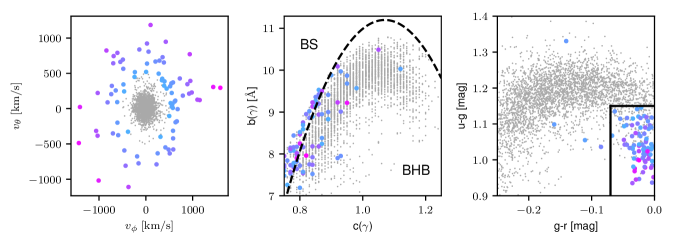
Figure 3: Kinematic and Spectral Parameters of the BHB sample after Removal of Sgr Stream Contaminants. Left Panel: We show the distribution of Galactocentric tangential velocities. Stars with total tangential velocity greater than 500 kms^-1 are plotted as large points in purple. The color of the points indicates the magnitude of their tangential velocity, with more pink being higher velocity. Middle Panel: We show the distribution of the BHB stars in the space of the scale width, $b(\gamma)$, of the H$\gamma$ line versus the line’s shape, $c(\gamma)$. The black dotted line is the dividing line used in Deason et al. (2011) to divide Blue Stragglers (BSs) from BHBs (although this was in the space of $b$ vs. $c$ for the combined parameters across the H$\gamma$, H$\delta$, and H$\beta$ lines). We see that the higher velocity stars lie preferentially on the BS side of this dividing line. Right Panel: We show the distribution of the BHBs in SDSS color-color space, where apparent high-velocity stars clearly lie preferentially in one corner of the diagram. According to Deason et al. (2011), this is exactly the region of color-color space where we expect BS contamination to be highest. Motivated by this, we exclude all stars within the black-box from our study.

3 Analysis

We now wish to understand how the velocity ellipsoid evolves as a function of Galactocentric radius. In order to account for the measurement errors, we implement a Gaussian deconvolution of the data performed in velocity space augmented by metallicity.

We take a relatively simple approach to this deconvolution by considering only four bins in Galactocentric radius. Motivated by the work of Belokurov et al. (2018) and Deason et al. (2018), we place the edge of our last bin at just beyond the apocenter of the ancient, massive, radial accretion event suggested by these works. We choose the other bin edges so that the first three bins have roughly the same number of stars. The edges of these four bins are $r=4.9,13.1,19.2,30,67.93$ kpc, the first and last edges being set by the limits of the data. These bins contain 880, 895, 884, and 405 stars, respectively. Since we are using relatively large distance bins and the BHBs have small photometric distance errors, the artificial movement of stars between bins due to distance uncertainties should be negligible.

We investigate two different deconvolutions of our data. The first implements a single Gaussian, while the second implements a version of a Gaussian Mixture Model (GMM) informed by the works of Belokurov et al. (2018), Myeong et al. (2018b), Lancaster et al. (2018) and Deason et al. (2018). In all of our fits, we define a likelihood function (a single Gaussian in the first case, a sum of Gaussians in the second) and sample the resulting posterior using the program emcee, which is an implementation of Goodman and Weare’s Affine Invariant Markov Chain Monte Carlo Sampler (Goodman & Weare, 2010; Foreman-Mackey et al., 2013). For both cases, we use 200 walkers and use 2000 steps as our ‘burn-in,’ followed by 2000 steps to explore the parameter space. We additionally verify the validity of our fitting code on fake generated data.

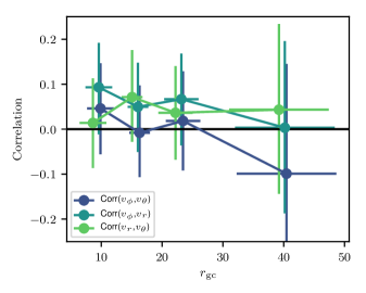
Figure 4: Evolution of the correlation coefficients between the different Galactocentric spherical-polar velocities. The correlation between two random variables $X$ and $Y$ is defined here as Corr$(X,Y)$=Cov$(X,Y)$/$\sqrt{{\rm Var}(X){\rm Var}(Y)}$. We illustrate these quantities instead of the tilt of the velocity ellipsoid as these parameters remain small even when the ellipsoid has nearly equal variance in two given directions. Note that the radial bins are artificially offset so that the errorbars are easier to observe. These errorbars span the 16th to the 84th percentiles of the 1d posteriors in each of these parameters.

3.1 Single Gaussian Model

We fit each of the four Galactocentric distance bins with a Gaussian distribution whose means, variances, and covariances in all dimensions are free parameters (except for covariances between metallicity and velocity space, which are set to zero). We additionally include an outlier component that consists of a single Gaussian. This outlier component is isotropic in the space of Galactocentric tangential velocities, and the width of the Gaussian in this space is allowed to vary as a free parameter, $\sigma_{\rm out}$. The properties of the outlier in the space of radial velocity and metallicity take fixed values, described further below. We include this component to account for any further contamination from Blue Stragglers, which will have much larger tangential velocity dispersion than the rest of our sample. Our fit to each bin then has 13 free parameters: the mean velocities $\mu_{v_{r}},\mu_{v_{\theta}}$ and $\mu_{v_{\phi}}$, the dispersions $\sigma_{v_{r}},\sigma_{v_{\theta}}$ and $\sigma_{v_{\phi}}$, and the covariances (‘tilt’) in these velocities Cov$(v_{\theta},v_{r})$, Cov$(v_{\phi},v_{r})$ and Cov$(v_{\phi},v_{\theta})$, the mean metallicity $\mu_{\rm[Fe/H]}$, the dispersion in metallicity $\sigma_{\rm[Fe/H]}$, the dispersion in tangential velocity of the isotropic, zero-mean outlier distribution $\sigma_{\rm out}$, and the fraction of outlier contamination $f_{\rm out}$.

Parameter	Priors	$r=4.9-13.1$ kpc	$r=13.1-19.2$ kpc	$r=19.2-30.0$ kpc	$r=30.0-67.93$ kpc
$\mu_{v_{\phi}}$ [km/s]	-	$0.51^{+3.18}_{-3.18}$	$7.42^{+2.76}_{-2.77}$	$0.88^{+2.79}_{-2.72}$	$6.81^{+5.01}_{-4.97}$
$\mu_{v_{\theta}}$ [km/s]	-	$7.12^{+2.99}_{-3.03}$	$9.23^{+2.68}_{-2.72}$	$3.91^{+2.44}_{-2.42}$	$15.28^{+5.38}_{-5.35}$
$\mu_{v_{r}}$ [km/s]	-	$-10.89^{+4.52}_{-4.76}$	$-0.09^{+4.10}_{-4.25}$	$-5.03^{+3.48}_{-3.50}$	$-5.69^{+4.89}_{-4.88}$
$\sigma_{v_{\phi}}$ [km/s]	[0,400]	$95.01^{+2.33}_{-2.28}$	$81.07^{+2.03}_{-1.94}$	$79.38^{+2.16}_{-2.03}$	$79.81^{+4.59}_{-4.37}$
$\sigma_{v_{\theta}}$ [km/s]	[0,400]	$87.84^{+2.11}_{-2.07}$	$81.64^{+2.01}_{-1.94}$	$69.62^{+1.92}_{-1.81}$	$85.82^{+4.68}_{-4.47}$
$\sigma_{v_{r}}$ [km/s]	[0,400]	$140.09^{+3.39}_{-3.28}$	$123.90^{+2.99}_{-2.91}$	$104.94^{+2.54}_{-2.47}$	$96.57^{+3.54}_{-3.44}$
Corr$(v_{\phi},v_{\theta})$	[-0.5,0.5]	$0.05^{+0.03}_{-0.03}$	$-0.01^{+0.03}_{-0.04}$	$0.02^{+0.04}_{-0.04}$	$-0.10^{+0.08}_{-0.08}$
Corr$(v_{\phi},v_{r})$	[-0.5,0.5]	$0.09^{+0.03}_{-0.03}$	$0.05^{+0.03}_{-0.03}$	$0.07^{+0.03}_{-0.03}$	$0.00^{+0.06}_{-0.06}$
Corr$(v_{r},v_{\theta})$	[-0.5,0.5]	$0.01^{+0.03}_{-0.03}$	$0.07^{+0.03}_{-0.03}$	$0.04^{+0.03}_{-0.03}$	$0.04^{+0.06}_{-0.06}$
$\mu_{\rm[Fe/H]}$ [dex]	[-3,0]	$-1.72^{+0.01}_{-0.01}$	$-1.75^{+0.01}_{-0.01}$	$-1.75^{+0.01}_{-0.01}$	$-1.84^{+0.02}_{-0.02}$
$\sigma_{\rm[Fe/H]}$ [dex]	[0,4]	$0.19^{+0.01}_{-0.01}$	$0.20^{+0.01}_{-0.01}$	$0.20^{+0.01}_{-0.01}$	$0.22^{+0.02}_{-0.02}$
$\sigma_{\rm out}$ [km/s]	[500,3000]	$1601.65^{+943.50}_{-834.21}$	$1594.84^{+953.75}_{-847.71}$	$1263.46^{+1115.13}_{-638.11}$	$1315.08^{+1069.54}_{-666.18}$
$f_{\rm out}$	[0,0.01]	$0.0009^{+0.0015}_{-0.0007}$	$0.0010^{+0.0016}_{-0.0007}$	$0.0012^{+0.0021}_{-0.0009}$	$0.0025^{+0.0034}_{-0.0018}$
$\ln\mathcal{L}_{\rm med}$	-	-16260.83	-16279.96	-15865.73	-7556.01

Table 1: Priors and Posterior estimates on all parameters in the single Gaussian fit, with outlier model. All priors are uniform within the bounds quoted, those without bounds, we place no prior on. Values quoted are 16th, 50th, and 84th percentiles of the 1d PDF in each parameter. In the last row we quote the likelihood values evaluated at the 1d medians in each parameter in each bin.

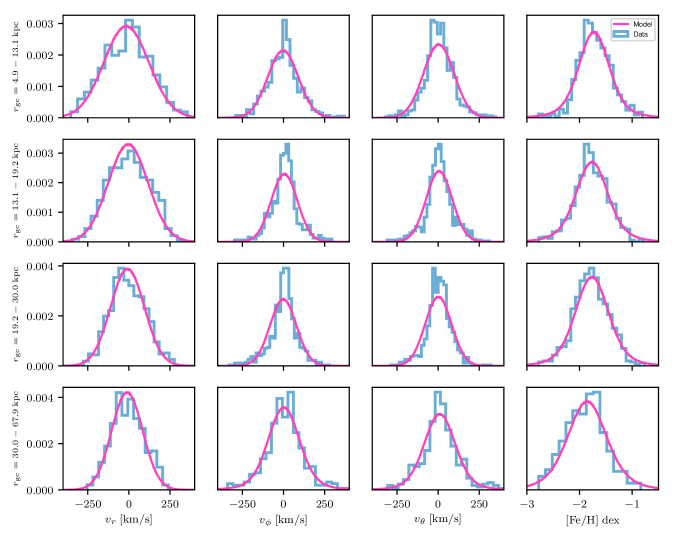
Figure 5: The single Gaussian fit to the Velocity Distributions. We show the results of independently fitting each of our four distance bins, allowing for variation in all parameters of the distribution save for covariance between the velocity components and metallicity. These bins contain 880, 895, 884, and 405 stars, respectively. We compare our model to the data by sampling from our best-fit model (specified by 1-D posterior medians) and convolving each sampled point with a randomly selected error from the data. This should provide a fair way of comparing the model with the data and takes into account the uncertainties. It is clear from the tangential velocity distributions that the data distribution is not well-fit by a single Gaussian. Note that since the outlier model has a negligible contribution, we do not show it here.

We do not assume alignment of the dispersion tensor in spherical polars. In fact, the alignment of the velocity dispersion tensor is an important diagnostic of the gravitational potential (Smith et al., 2009b; An & Evans, 2016). From earlier studies based on samples of halo stars with noisier proper motions, the covariance of velocities in spherical polar or tilt is believed to be small (e.g., Smith et al., 2009b; Evans et al., 2016). This seems to be true of the RR Lyrae population in the stellar halo, which has been recently analysed using Gaia DR2 proper motion data by Wegg et al. (2018). We independently see that this is the case in the BHBs. This result is illustrated in Fig. 4, which shows the evolution of the correlations between the different velocity components as a function of Galactocentric radius. We see that the correlations are consistent with zero at all radii.

The likelihood for this model, $\mathcal{L}(\mathbf{D}|\boldsymbol{\theta})$, where $\mathbf{D}$ is the vector of all data points, and $\boldsymbol{\theta}$ is the vector of model parameters, is given by:

$$\mathcal{L}(\mathbf{D}|\boldsymbol{\theta})=\prod_{i}\sum_{j={\rm d,o}}f_{j}\mathcal{L}_{j}(D_{i}|\boldsymbol{\theta})$$ (4)

Here, the product index $i$ runs over all data points and the sum index $j$ runs over the two different components of the model (1) the ‘data’ component, denoted by a subscript d and (2) the ‘outlier’ component denoted by a subscript o. Also, $f_{j}$ is the fraction of component $j$ that makes up the total data set. We then have the likelihoods for the components defined as:

$$\mathcal{L}_{\rm d}(D_{i}|\boldsymbol{\theta})=\mathcal{N}\left(\mathbf{v}_{i}|\boldsymbol{\mu},\boldsymbol{\Sigma}_{i}^{\rm d}\right)\mathcal{N}\left({\rm[Fe/H]}_{i}|\mu_{\rm[Fe/H]},\sigma_{{\rm[Fe/H]},i}\right)$$ (5)

where $\mathcal{N}$ denotes a normal distribution, $\mathbf{v}_{i}$ is the velocity of data point $i$ in Galactocentric spherical polar coordinates, $\boldsymbol{\mu}\equiv(\mu_{v_{\phi}},\mu_{v_{\theta}},\mu_{v_{r}})$ is the mean in velocity space of the single Gaussian. The full covariance matrix in velocity space $\boldsymbol{\Sigma}_{i}^{\rm d}$ is a sum of the covariance matrix from measurement error $\boldsymbol{\Sigma}_{i}$ and the covariance matrix of the model being fit $\boldsymbol{\Sigma}^{\rm d}$. Additionally, [Fe/H]_i is the metallicity of data point $i$, while $\mu_{{\rm[Fe/H]}}$ and $\sigma_{{\rm[Fe/H],i}}$ are the mean and dispersion. Again, the latter quantity is a combination (in quadrature) of the individual measurement error and the standard deviation of the model.

The outlier component of the model is relatively rigid, its properties being described solely by its fractional contribution and dispersion in tangential velocity. Its likelihood is defined as:

$$\mathcal{L}_{\rm o}(D_{i}|\boldsymbol{\theta})=\mathcal{N}\left(\mathbf{v}_{i}|\boldsymbol{0},\boldsymbol{\Sigma}_{i}^{\rm o}\right)\mathcal{N}\left({\rm[Fe/H]}_{i}|\mu_{\rm[Fe/H]},\sigma_{{\rm[Fe/H]},i}\right)$$ (6)

where $\mathbf{v}_{i}$ is the velocity of data point $i$, $\boldsymbol{0}$ denotes that the outlier has zero mean in the velocity space, and $\boldsymbol{\Sigma}_{i}^{\rm o}\equiv\boldsymbol{\Sigma}_{i}+\boldsymbol{\Sigma}^{\rm o}$ is the covariance matrix of the distribution which is a combination of measurement error in the velocity space $\boldsymbol{\Sigma}_{i}$ and the width of the outlier component $\boldsymbol{\Sigma}^{\rm o}\equiv{\rm diag}\left(\sigma_{\rm out}^{2},\sigma_{\rm out}^{2},\sigma_{r,{\rm out}}^{2}\right)$, where $\sigma_{r,{\rm out}}$ is the dispersion in the radial velocity space and is set to 150 km/s and $\sigma_{{\rm out}}$ is the dispersion in the tangential velocity space and is allowed to vary as a free parameter of the fit. The parameters of the outlier component in metallicity space are also fixed throughout the fit $\mu_{\rm[Fe/H]}=-1.75$, and $\sigma_{{\rm[Fe/H]},i}=0.2$.

We additionally note that our single Gaussian Model picks out the velocity ellipsoid to be essentially isotropic in the tangential velocity space (i.e. $\sigma_{v_{\theta}}=\sigma_{v_{\phi}}$) at all Galactocentric radii. This can be seen from the results in Table 1. This observation motivates the simplification of the description of the space of tangential velocities in our next model.

Parameter	Priors	$r=4.9-13.1$ kpc	$r=13.1-19.2$ kpc	$r=19.2-30.0$ kpc	$r=30.0-67.93$ kpc
$\mu_{v_{\phi},{\rm r}}$ [km/s]	-	$-4.49^{+4.55}_{-4.41}$	$11.54^{+2.25}_{-2.26}$	$14.13^{+2.31}_{-2.30}$	$-27.39^{+56.40}_{-73.68}$
$\mu_{\rm[Fe/H],h}$ [dex]	[-3,0]	$-1.82^{+0.03}_{-0.02}$	$-1.88^{+0.01}_{-0.01}$	$-1.85^{+0.02}_{-0.02}$	$-1.86^{+0.02}_{-0.02}$
$\mu_{\rm[Fe/H],r}$ [dex]	[-3,0]	$-1.62^{+0.02}_{-0.02}$	$-1.60^{+0.02}_{-0.02}$	$-1.62^{+0.02}_{-0.02}$	$-1.29^{+0.10}_{-0.13}$
$\sigma_{\rm[Fe/H],h}$ [dex]	[0,4]	$0.10^{+0.04}_{-0.05}$	$0.09^{+0.03}_{-0.04}$	$0.15^{+0.02}_{-0.02}$	$0.17^{+0.04}_{-0.06}$
$\sigma_{\rm[Fe/H],r}$ [dex]	[0,4]	$0.21^{+0.02}_{-0.02}$	$0.18^{+0.02}_{-0.02}$	$0.17^{+0.02}_{-0.02}$	$0.12^{+0.20}_{-0.09}$
$\sigma_{v_{r},{\rm h}}$ [km/s]	[0,400]	$129.24^{+5.69}_{-5.46}$	$122.03^{+4.38}_{-4.25}$	$113.62^{+4.09}_{-3.83}$	$95.21^{+3.56}_{-3.72}$
$\sigma_{t,{\rm h}}$ [km/s]	[0,400]	$114.27^{+4.58}_{-4.32}$	$105.41^{+3.00}_{-2.76}$	$96.72^{+3.03}_{-3.00}$	$79.33^{+3.57}_{-3.44}$
$\sigma_{v_{r},{\rm r}}$ [km/s]	[0,400]	$109.93^{+11.91}_{-7.91}$	$78.21^{+5.13}_{-4.43}$	$62.91^{+7.50}_{-5.13}$	$176.36^{+87.76}_{-53.12}$
$\sigma_{t,{\rm r}}$ [km/s]	[0,400]	$58.18^{+3.78}_{-4.57}$	$34.02^{+1.78}_{-1.71}$	$29.14^{+2.04}_{-1.86}$	$145.69^{+47.78}_{-30.27}$
$\delta_{\rm out}$ [km/s]	[0,500]	$104.16^{+11.84}_{-16.81}$	$98.60^{+5.25}_{-5.64}$	$67.75^{+5.28}_{-6.82}$	$82.87^{+57.31}_{-54.80}$
$f_{\rm h}$	[0.01,0.99]	$0.52^{+0.07}_{-0.06}$	$0.55^{+0.03}_{-0.03}$	$0.55^{+0.03}_{-0.03}$	$0.96^{+0.02}_{-0.04}$
$\ln\mathcal{L}_{\rm med}$	-	$-16205.77$	$-16084.97$	$-15714.09$	$-7552.66$

Table 2: Priors and Posterior estimates on all parameters in the Gaussian Mixture Model fit. All priors are uniform within the bounds quoted, those without bounds, we place no prior on. Values quoted are 16th, 50th, and 84th percentiles of the 1d PDF in each parameter. In the last row we quote the likelihood values evaluated at the 1d medians in each parameter in each bin.

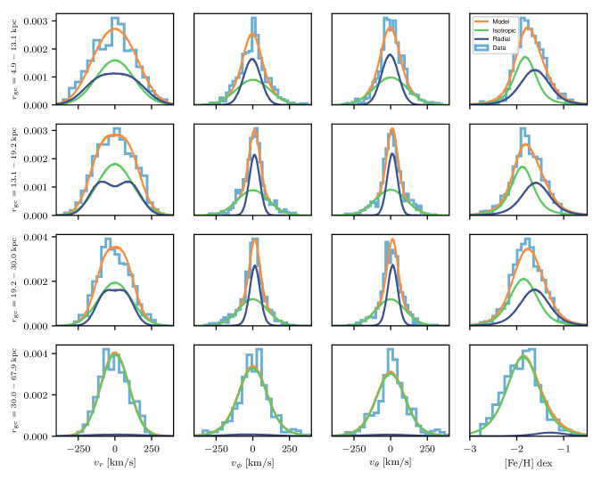
Figure 6: The Gaussian Mixture Model (GMM) Fit. We show the results of independently fitting each of our four distance bins, allowing for variation in all parameters of the model. These bins contain 880, 895, 884, and 405 stars, respectively. Similarly to Fig. 5, in order to compare data to model, we sample from our best fit model and convolve each sampled point with a randomly selected error from the data set.

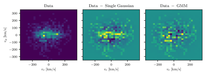
Figure 7: Comparison of Fit Residuals in Plane of Velocities. We show residuals in the plane of radial velocity versus azimuthal velocity for our 2 models when fit to the data in our third Galactocentric distance bin ($r_{\rm gc}=19.2-30$ kpc), where the differences are most clear. The “Data" histogram was constructed using 884 stars, and the histogram has 30 bins on each side, meaning that a uniform distribution would correspond to $\sim$1 star per bin. Bright Yellow corresponds to the model under-predicting the number of stars in the bin by 5 stars, while Dark Blue corresponds to the model over-predicting the number of stars in that bin by 5. Left Panel: Histogram of the Data. Middle Panel: The residuals of the single Gaussian model, which clearly under-predicts the density at low $|v_{\phi}|$. Right Panel: The residuals of the Gaussian Mixture Model fit.

3.2 Gaussian Mixture Model

Our second model is a Gaussian Mixture Model (GMM) (Press et al., 2007) that is motivated by the results of several recent works which have suggested that the stellar halo could be largely dominated by a single, ancient, extremely radial merger (Belokurov et al., 2018; Myeong et al., 2018a, b; Deason et al., 2018; Kruijssen et al., 2018; Helmi et al., 2018). Our mixture model consists of two components, one representing the more metal-poor, largely isotropic stellar halo, and the other representing the more metal-rich, radially anisotropic stars from the putative massive, accretion event (the “Sausage”). This dichotomy is clearly seen in the plots of the stellar halo in action space at different metallicities presented in e.g. Belokurov et al. (2018) and Myeong et al. (2018b). In the mixture model, anticipating the insights gained from the results of our single Gaussian fit, we do not include any outliers, nor do we allow any tilt in the velocity ellipsoid. These assumptions significantly reduce the complexity of the model, speeding our calculations and helping avoid possible degeneracies that could arise from a large number of parameters.

The first of our two components is a single Gaussian, meant to represent the large isotropic portion of the halo, with zero mean in all velocity components and whose velocity tensor in the tangential direction is enforced to be isotropic ($\sigma_{t,{\rm h}}\equiv\sigma_{v_{\phi}}=\sigma_{v_{\theta}}$). We additionally allow the mean metallicity $\mu_{\rm[Fe/H],h}$, metallicity dispersion $\sigma_{\rm[Fe/H],h}$, and fractional contribution of this component, $f_{\rm h}$, to vary. This then leaves five free parameters describing this component $\{\sigma_{t,{\rm h}},\sigma_{v_{r},{\rm h}},\mu_{\rm[Fe/H],h},\sigma_{\rm[Fe/H],h},f_{\rm h}\}$.

The second - or the “Sausage” - component is built from two Gaussians with equal mixing fraction, which are identical except for their mean radial velocities. They are set as $\mu_{v_{r},1}=+\delta$ and $\mu_{v_{r},2}=-\delta$, where the radial velocity separation $\delta$ is treated as a free parameter in the fit. This heuristic model mimics the behaviour found in the local sample of SDSS-Gaia stars from Belokurov et al. (2018), in which, after subtracting a zero-mean Gaussian Mixture model, there are distinct ‘lobes’ at high positive and high negative radial velocity. Our parameterization has a simple physical explanation. If a component of the stellar halo is well-mixed and highly radially anisotropic, then the velocity distribution of the stars can still be Gaussian to a good approximation at any spot (e.g., Osipkov, 1979; Merritt, 1985; Evans & An, 2006). However, if the component comes from a single accretion event, then a sample restricted to a small volume lying between the apocenters and pericenters of stars from the accretion event will be missing the stars ‘turning around’ on their orbits. Thus, we will only observe stars at large negative (incoming) or positive (outgoing) radial velocity. The two ‘lobes’ are expected to be overlapping near the peri and the apo of the debris and move further apart in between the turning points. Given the fact that the orbital velocities increase towards the Galactic Center, combined with the action of the apsidal precession, the maximal separation between the lobes is likely attained at small Galactocentric radii.

For this Sausage component, in addition to $\delta$, we then have the following free parameters representing the shape of each of the two Gaussians: the radial velocity dispersion $\sigma_{v_{r},{\rm r}}$, the tangential velocity dispersion, $\sigma_{t,{\rm r}}\equiv\sigma_{v_{\phi}}=\sigma_{v_{\theta}}$, the mean metallicity $\mu_{\rm[Fe/H],r}$, and metallicity dispersion $\sigma_{\rm[Fe/H],r}$. We also allow for mean rotation $\mu_{v_{\phi},{\rm r}}$ in this component, motivated by the findings of Belokurov et al. (2018), Helmi et al. (2018), and Myeong et al. (2018b), giving us six free parameters.

We then have the likelihood for this GMM defined similarly to Eq.  (4) as:

$$\mathcal{L}(\mathbf{D}|\boldsymbol{\theta})=\prod_{i}\sum_{j={\rm r,h}}f_{j}\mathcal{L}_{j}(D_{i}|\boldsymbol{\theta})$$ (7)

where $i$ is again a product over the data points, and $j$ is a sum over the different components of the model (r for the radially anisotropic component and h for the isotropic halo component), while $f_{j}$ denotes the fractional contribution from component $j$.

The likelihood of the isotropic halo component is given by:

$$\mathcal{L}_{\rm h}\left(D_{i}|\boldsymbol{\theta}\right)=\mathcal{N}\left(\mathbf{v}_{i}|\boldsymbol{0},\boldsymbol{\Sigma}_{i}^{\rm h}\right)\mathcal{N}\left({\rm[Fe/H]}_{i}|\mu_{\rm[Fe/H],{\rm h}},\sigma_{{\rm[Fe/H]},i}\right)$$ (8)

where the velocities are normally distributed about zero mean with a covariance matrix $\boldsymbol{\Sigma}_{i}^{\rm h}$ which is a combination of measurement error and the intrinsic dispersions.

The likelihood of the radially anisotropic or Sausage component is a bit more complicated. It is given by:

$$\mathcal{L}_{\rm r}\left(D_{i}|\boldsymbol{\theta}\right) = \left[\tfrac{1}{2}\mathcal{N}\left(\mathbf{v}_{i}|\boldsymbol{\mu}_{1},\boldsymbol{\Sigma}_{i}^{\rm r}\right)+\tfrac{1}{2}\mathcal{N}\left(\mathbf{v}_{i}|\boldsymbol{\mu}_{2},\boldsymbol{\Sigma}_{i}^{\rm r}\right)\right]$$ (9)

$$\times \mathcal{N}\left({\rm[Fe/H]}_{i}|\mu_{\rm[Fe/H],r},\sigma_{{\rm[Fe/H]},i}\right)$$

where the means are $\mu_{1}\equiv\left(\mu_{v_{\phi}},0,\delta\right)$, $\mu_{2}\equiv\left(\mu_{v_{\phi}},0,-\delta\right)$, and the covariance of the Gaussian $\boldsymbol{\Sigma}_{i}^{\rm r}$ is a combination of the measurement error $\boldsymbol{\Sigma}_{i}$ and the intrinsic dispersions $\boldsymbol{\Sigma}^{r}\equiv{\rm diag}\left(\sigma^{2}_{v_{\phi}},\sigma^{2}_{v_{\phi}},\sigma^{2}_{v_{r}}\right)$. We then fit each Galactocentric distance bin individually using the above likelihood. We do not require the Sausage component to have a larger radial velocity dispersion than the isotropic component, nor do we impose any requirement that it is of higher metallicity. We adopt very conservative (unifrom) priors for each parameter in our fit and allow for each of these characteristics to arise from the fit.

For the single-Gaussian component fit to the data there are a total of 52 free parameters (13 for each of the four distance bins) while for the two-component model there are 44 free parameters (11 for each of the four distance bins). Therefore, due to restrictions imposed on the two-component model, it actually has fewer degrees of freedom than the single Gaussian model, making it a priori less susceptible to over-fitting.

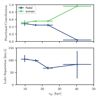
Figure 8: The Behavior of the components in the GMM fit with Galactocentric distance. Values shown are 1-D medians of the given parameter over the posterior, the errors are based on th 16-th and 84-th percentiles of the 1-D posterior distribution. Top panel: We show the evolution of the fractional contribution of the two components. Note that the radially anisotropic or Sausage component falls off dramatically beyond $\sim 20$ kpc. Bottom panel: We show how the separation of the lobes in Galacto-centric radial velocity of the Sausage changes.

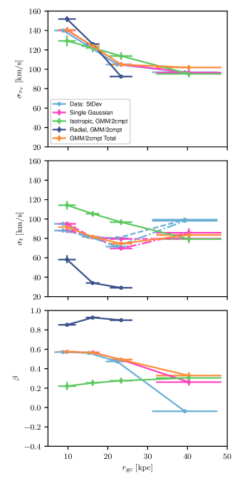
Figure 9: Radial Evolution of the Kinematic Properties of the Halo. Light green lines represent the isotropic component of the GMM, while the dark blue represents the Sausage component. Orange lines represent the measurement from the combination of two components. Pink lines represent the results for the single Gaussian model. Finally light blue lines are used for quantities calculated directly from standard deviations of the data, including sigma clipping, and compensating for measurement error in quadrature. Values shown are 1-D medians of the given parameter over the posterior, the errors are based on th 16-th and 84-th percentiles of the 1-D posterior distribution. Top Panel: Radial velocity dispersion with Galactocentric radius. Middle Panel: Tangential velocity dispersions. For the ‘Data’ and the ‘Single Gaussian’ models there is a difference between the dispersion in the polar velocity $\sigma_{v_{\theta}}$ and the azimuthal velocity $\sigma_{v_{\phi}}$, these are shown separately as the dash-dotted and dotted lines, respectively. Bottom Panel: We show the evolution of the radial anisotropy parameter, defined by Eq. 1.

4 Results

After sampling the model parameters using emcee, we obtain their posterior distribution functions (PDFs), which have only a single mode and have shapes very close to Gaussian. In Tab.  1 and 2 we show the parameter estimates from our fits, quoted as the 16th, 50th, and 84th percentiles of the 1d posteriors in each parameter. For each model parameter, we use the median (50th percentile) of the 1d PDF as a parameter estimate. To assess the performance of the model against the data, we use these estimated best-fit parameters to sample the model and convolve each sampled point with a Gaussian error sampled randomly from the data set. The resulting predictive distributions can be compared to the data in Fig. 5, 6, and 7.

Upon inspection of Fig. 5, it is clear that the distribution of the data is not well explained by a single Gaussian component. This is most evident in the distributions of tangential velocities. Especially in the inner three radial bins, the central regions of the distribution exhibit strong deviations from the best-fit model.

Fig. 6 clearly shows that the 2-component mixture model is a much better fit to the shape of the velocity ellipsoid, especially in the inner halo $r<30$ kpc. More quantitatively, one can tell that the 2-component mixture model provides a better fit to the data from parameters provided in the bottom row of Tables 1 and 2: the difference of the sum of the likelihoods over all distance bins is $\ln\left(\mathcal{L}_{\rm med,GMM}\right)-\ln\left(\mathcal{L}_{\rm med,single}\right)=405$ despite the smaller number of parameters in the mixture model. We enforce no constraint that requires the Sausage component to be dynamically colder in the tangential velocities: this comes out naturally from the fit. Similarly, the Sausage is naturally chosen to be more metal-rich by our fit. This is despite the fact that BHBs are naturally more metal-poor objects, making our measurement biased against the Sausage component which is metal-rich (Belokurov et al., 2018). At the moment, the best unbiased estimates of the metallicity distribution of the Sausage are those using main sequence stars such as Necib et al. (2018) and Belokurov et al. (2018), which suggest mean metallicities of about [Fe/H]$\approx-1.4$, but also indicate that the distribution is broad and extends well into the metallicities probed in this study. So, though it is likely that our use of a metal-poor tracer will bias our estimate of the fractional contribution to the Sausage to the stellar halo, we can still clearly demonstrate that the Sausage makes up a large fraction of our sample.

In Fig. 7 we show the residuals of our two models in the plane of Galactocentric radial velocity versus Galactocentric azimuthal velocity in the third Galactocentric distance bin ($r_{\rm gc}=19.2-30$ kpc). This comparison further illustrates the failings of the single Gaussian model as well as the reason why the ‘sausage’ component is picked out to be the tangentially cold component in our GMM fit.

Another indication that this model makes good physical sense is the behavior of the parameters of the fit as a function of radius, as shown in Fig. 8. The fractional contribution of the Sausage falls sharply at distances beyond 20 kpc, as the isotropic component becomes dominant. This corresponds to the proposed apocentric pile-up of stars connected with the ancient, radial accretion event (e.g., Deason et al., 2018). The velocity separation of the lobes also decreases with increasing radius. This is expected from the physical interpretation of the lobes as the infalling and outgoing parts of a highly eccentric merger event. The lobes attain the furthest separation close to the Galactic Center, when the stars are moving the fastest. They then approach each other on moving outwards, essentially totally overlapping with one another in the third distance bin. According to this interpretation, we would expect the isotropic component to become completely dominant beyond the apocenter radius $\sim 20-30$ kpc and the $\delta$ parameter to therefore become largely unconstrained, which is exactly what we see.

In Fig. 9, we summarize the kinematic properties of the Milky Way’s stellar halo inferred from the fits. We display how the velocity dispersions in the radial and tangential directions evolve for our four different distance bins. In light blue, the quantities predicted are calculated by computing the standard deviation in each velocity component directly from the data  (and subtracting the mean velocity error in quadrature, cf Bird et al., 2018). Note that to do this measurement we also perform ‘sigma-clipping’ whereby we recursively remove any star that lies outside of 4$\sigma$ according to the calculated standard deviation. This helps to beat down the contamination by outliers such as Blue Stragglers. We then show the quantities inferred by our single Gaussian Model (in pink), along with each component of the GMM (isotropic in light green and radial in dark blue). Finally, the orange curve gives the combination of both components in the GMM model, which is derived from sampling the parameters of the GMM model.

There are two main points to be made. The first comes from a comparison of the dispersion calculated directly from the data (when mean error is subtracted in quadrature), and that inferred from deconvolution. The lesson to be learned here is that taking measurement error in to account (in a rigorous way) when performing calculations such as these is important and can lead to different answers, especially when the errors are large or when the dataset contains a mixture of points with wide range of uncertainties. In fact, testing this method on fake data, generated to have similar errors to those found in our last Galactocentric distance bin, we found that simple dispersion-based method underestimated $\beta$ by about 0.4. The second point here is, surprisingly, that changing the underlying model being fit to the data does not result in drastically different estimates of the second moments of the velocity ellipsoid. While our GMM model is clearly a much better fit to the data, it predicts generally the same velocity dispersions as the single Gaussian fit. This is most likely due to the fact that the contribution of the two components of our GMM is either nearly equal (inner halo) or completely dominated by one component (outer halo), meaning that a single Gaussian fit would try to fit equally between the two components, resulting in a similar velocity dispersion.

5 Conclusions

We have assembled a high-purity set of blue horizontal branch stars (BHBs) with spectroscopic data from the Sloan Digital Sky Survey and astrometric data courtesy of the Gaia satellite. The sample of 3 064 BHBS has seven dimensional phase space information (positions, velocities and metallicities). This enables the kinematic properties of the BHBs in the Milky Way halo to be studied out to $\sim 40$ kpc.

Traditionally, the stellar halo has often been represented by a single distribution function (e.g., Posti et al., 2015; Williams & Evans, 2015). The underlying assumption is that the stars are well-mixed and relaxed in a steady potential. However, it has perhaps never been entirely clear that stellar halos satisfy such requirements. The time taken for stars in the outer parts of galaxies to exchange angular momenta with each other is longer than a Hubble time, so unrelaxed structures are expected to be abundant.

Nonetheless, if the velocity distributions of the BHB stars are fitted with a single Gaussian with spatially varying dispersions, then some interesting conclusions can be obtained. First, the tilt angles or covariances are small. The velocity dispersion tensor is closely aligned with the spherical polar coordinate system. This result has been seen before with poorer quality proper motion data (Smith et al., 2009b; Evans et al., 2016) and has recently been confirmed in the inner halo by Wegg et al. (2018) for a large sample of 15651 RR Lyrae with accurate proper motions from Gaia data release 2 (DR2). The only non-singular potential for which spherical alignment occurs everywhere is spherically symmetric (Smith et al., 2009b; An & Evans, 2016). Secondly, the best single Gaussian fit confirms that the stellar halo is radially anisotropic. Although the dispersions evolve with radius, the anisotropy parameter is constant at $\beta\approx 0.6$ in the inner halo, dropping to values of 0.3 beyond the proposed apocenter of the Gaia Sausage. The radial velocity dispersion $\sigma^{2}_{v_{r}}$ is largest. Although $\sigma^{2}_{v_{\phi}}$ and $\sigma^{2}_{v_{\theta}}$ can be different, the best fit usually has the two angular dispersions the same within $1\sigma$. This also suggests that the potential is close to spherical.

The data however exhibit significant deviations from a single Gaussian velocity distribution. The central regions of the angular velocity distributions, especially in the inner halo, are not well-matched. This contributes to the emerging picture of the Milky Way’s stellar halo as possessing multiple unrelaxed components and motivated us to seek a new model. We devised a Gaussian Mixture Model (GMM) of an unusual form, using the insights supplied by Myeong et al. (2018b), Deason et al. (2018), and Belokurov et al. (2018) in their studies of the halo in action space, orbital elements space, and velocity space respectively. The first component of the GMM is an isotropic Gaussian with dispersions aligned in spherical polar coordinates. Although we make no assumptions about its metallicity, our choice is inspired by the largely isotropic metal-poor halo (e.g., Myeong et al., 2018b). The second component is built from a sum of two Gaussians, each one of which mimics the lobes of the velocity distribution of the “Gaia Sausage" seen by Belokurov et al. (2018). The Gaussians are radially anisotropic and have means in Galactocentric radial velocity separated by $\delta$ to represent the incoming and outgoing parts of an unrelaxed structure created by the remote infall of a dwarf galaxy. Note that a very similar modelling approach has been recently applied to the local halo data by Necib et al. (2018).

The GMM provides a better match to the data. In particular, the Sausage component is dynamically colder in the tangential velocities than the isotropic component. Similarly, the Sausage component is more metal-rich than the isotropic component. These properties emerge naturally from the fit, but are in good agreement with previous attempts to characterize this ancient accretion event. The behaviour of the velocity offset between two lobes in the model also makes good physical sense. It is largest ($\delta\approx 100$ kms^-1) in the inner Galaxy, where we expect the stars to be moving fastest but having not reached pericenter yet, and it drops dramatically at distances of $\approx 20$ kpc. This is believed to mark the apocentres of the stars that once belonged to the Sausage Galaxy (Deason et al., 2018). This interpretation is further confirmed by the contribution of the Sausage component dropping dramatically beyond $\sim 30$ kpc, consistent with the results of Deason et al. (2011). Here, for the first time, we directly track the change in the stellar halo composition over a large range of radii. Our results strongly argue that the stellar halo of the Milky Way is in large part unrelaxed, even in its innermost parts.

Our model fit provides further evidence for the inner 30 kpc of the stellar halo of the Milky Way being in large part dominated by an ancient, massive, radial merger event. According to our models, this massive event contributed a significant fraction of the stellar halo’s mass. Its fractional contribution to the stellar halo varying as a function of radius, but it makes up $\sim 50\%$ of the metal-poor stellar halo in the inner 30 kpc. As our sample is biased towards metal-poor stars, and thus against the metal-rich Gaia Sausage (see Belokurov et al., 2018), this should really be viewed as a lower bound on the fractional contribution of this merger event to the overall halo contents. The prospects of larger datasets with seven-dimensional phase space information suggests elaborations of our work here will shortly be possible. In particular, it is unclear whether the Gaia Sausage is the residue of a single very radial in-fall, or two or more infalls, one prograde and one retrograde (c.f., Kruijssen et al., 2018). The methodology of this paper applied to the kinematics and chemistry of still larger samples of halo stars may enable further clues to be deduced about the remote history of our Galactic home.

References

- Aihara et al. (2011) Aihara H., et al., 2011, The Astrophysical Journal Supplement Series, 193
- An & Evans (2016) An J., Evans N. W., 2016, ApJ, 816, 35
- Battaglia et al. (2005) Battaglia G., et al., 2005, MNRAS, 364, 433
- Bekki & Chiba (2001) Bekki K., Chiba M., 2001, ApJ, 558, 666
- Belokurov et al. (2014) Belokurov V., et al., 2014, MNRAS, 437, 116
- Belokurov et al. (2018) Belokurov V., Erkal D., Evans N. W., Koposov S. E., Deason A. J., 2018, preprint, (arXiv:1802.03414)
- Bird et al. (2018) Bird S. A., Xue X.-X., Liu C., Shen J., Flynn C., Yang C., 2018, preprint, (arXiv:1805.04503)
- Bond et al. (2010) Bond N. A., et al., 2010, ApJ, 716, 1
- Bowden et al. (2016) Bowden A., Evans N. W., Williams A. A., 2016, MNRAS, 460, 329
- Chen et al. (2001) Chen B., et al., 2001, ApJ, 553, 184
- Chiba & Yoshii (1998) Chiba M., Yoshii Y., 1998, AJ, 115, 168
- Cui et al. (2012) Cui X.-Q., et al., 2012, Research in Astronomy and Astrophysics, 12, 1197
- Cunningham et al. (2016) Cunningham E. C., et al., 2016, ApJ, 820
- Das & Binney (2016) Das P., Binney J., 2016, MNRAS, 460, 1725
- Deason et al. (2011) Deason A. J., Belokurov V., Evans N. W., 2011, MNRAS, 416, 2903
- Deason et al. (2012) Deason A. J., Belokurov V., Evans N. W., An J., 2012, MNRAS, 424, L44
- Deason et al. (2013) Deason A. J., Belokurov V., Evans N. W., Johnston K. V., 2013, ApJ, 763, 113
- Deason et al. (2018) Deason A. J., Belokurov V., Koposov S. E., Lancaster L., 2018, ApJ, 862, L1
- Eggen et al. (1962) Eggen O. J., Lynden-Bell D., Sandage A. R., 1962, ApJ, 136, 748
- Evans & An (2006) Evans N. W., An J. H., 2006, Phys. Rev. D, 73, 023524
- Evans et al. (2016) Evans N. W., Sanders J. L., Williams A. A., An J., Lynden-Bell D., Dehnen W., 2016, MNRAS, 456, 4506
- Foreman-Mackey et al. (2013) Foreman-Mackey D., Hogg D. W., Lang D., Goodman J., 2013, PASP, 125, 306
- Frenk & White (1980) Frenk C. S., White S. D. M., 1980, MNRAS, 193, 295
- Gaia Collaboration et al. (2016) Gaia Collaboration et al., 2016, A&A, 595, A1
- Gaia Collaboration et al. (2018) Gaia Collaboration et al., 2018, A&A, 616, A1
- Gillessen et al. (2009) Gillessen S., Eisenhauer F., Trippe S., Alexander T., Genzel R., Martins F., Ott T., 2009, ApJ, 692, 1075
- Gnedin et al. (2010) Gnedin O. Y., Brown W. R., Geller M. J., Kenyon S. J., 2010, ApJ, 720, L108
- Goodman & Weare (2010) Goodman J., Weare J., 2010, Communications in Applied Mathematics and Computational Science, Vol.~5, No.~1, p.~65-80, 2010, 5, 65
- Helmi et al. (2018) Helmi A., Babusiaux C., Koppelman H. H., Massari D., Veljanoski J., Brown A. G. A., 2018, preprint, p. arXiv:1806.06038 (arXiv:1806.06038)
- Hernitschek et al. (2017) Hernitschek N., et al., 2017, ApJ, 850, 96
- Johnston et al. (2008) Johnston K. V., Bullock J. S., Sharma S., Font A., Robertson B. E., Leitner S. N., 2008, ApJ, 689
- Kafle et al. (2012) Kafle P. R., Sharma S., Lewis G. F., Bland-Hawthorn J., 2012, ApJ, 761
- Kafle et al. (2013) Kafle P. R., Sharma S., Lewis G. F., Bland-Hawthorn J., 2013, MNRAS, 430, 2973
- Kafle et al. (2017) Kafle P. R., Sharma S., Robotham A. S. G., Pradhan R. K., Guglielmo M., Davies L. J. M., Driver S. P., 2017, MNRAS, 470, 2959
- Kruijssen et al. (2018) Kruijssen J. M. D., Pfeffer J. L., Reina-Campos M., Crain R. A., Bastian N., 2018, MNRAS,
- Lancaster et al. (2018) Lancaster L., Belokurov V., Evans N. W., 2018, preprint, p. arXiv:1804.09181 (arXiv:1804.09181)
- Merritt (1985) Merritt D., 1985, AJ, 90, 1027
- Myeong et al. (2018a) Myeong G. C., Evans N. W., Belokurov V., Sanders J. L., Koposov S. E., 2018a, preprint, (arXiv:1805.00453)
- Myeong et al. (2018b) Myeong G. C., Evans N. W., Belokurov V., Sanders J. L., Koposov S. E., 2018b, ApJ, 856, L26
- Necib et al. (2018) Necib L., Lisanti M., Belokurov V., 2018, preprint, (arXiv:1807.02519)
- Osipkov (1979) Osipkov L. P., 1979, Soviet Astronomy Letters, 5, 42
- Posti et al. (2015) Posti L., Binney J., Nipoti C., Ciotti L., 2015, MNRAS, 447, 3060
- Press et al. (2007) Press W. H., Teukolsky S. A., Vetterling W. T., Flannery B. P., 2007, Numerical Recipes 3rd Edition: The Art of Scientific Computing, 3 edn. Cambridge University Press, New York, NY, USA
- Reid & Brunthaler (2004) Reid M. J., Brunthaler A., 2004, ApJ, 616, 872
- Schönrich et al. (2010) Schönrich R., Binney J., Dehnen W., 2010, MNRAS, 403, 1829
- Searle & Zinn (1978) Searle L., Zinn R., 1978, ApJ, 225, 357
- Sirko et al. (2004) Sirko E., et al., 2004, AJ, 127, 914
- Smith et al. (2009a) Smith M. C., et al., 2009a, MNRAS, 399, 1223
- Smith et al. (2009b) Smith M. C., Wyn Evans N., An J. H., 2009b, ApJ, 698, 1110
- The Astropy Collaboration et al. (2018) The Astropy Collaboration et al., 2018, preprint, (arXiv:1801.02634)
- Wegg et al. (2018) Wegg C., Gerhard O., Bieth M., 2018, preprint, (arXiv:1806.09635)
- Williams & Evans (2015) Williams A. A., Evans N. W., 2015, MNRAS, 454, 698
- Xue et al. (2008) Xue X. X., et al., 2008, ApJ, 684
- Xue et al. (2011) Xue X.-X., et al., 2011, ApJ, 738, 79