Abstract

We suppose that the observed neutrino masses can be parametrised by a lepton number violating dimension-five operator, and calculate the mixing of double insertions of this operator into lepton flavour changing dimension-six operators of the standard model effective theory. This allows to predict the log-enhanced, but $m_{\nu}^{2}$-suppressed lepton flavour violation that is generic to high-scale Majorana neutrino mass models. We also consider the Two Higgs Doublet Model, where the second Higgs allows the construction of three additional dimension-five operators, and evaluate the corresponding anomalous dimensions. The sensitivity of current searches for lepton flavour violation to these additional Wilson coefficients is then examined.

1 Introduction

Neutrinos are elusive and enigmatic particles: uncoloured, uncharged, and very light. Nonetheless, their observed masses and mixing angles [1] imply that Lepton Flavour Violation (LFV) must occur, where we define LFV as flavour-changing contact interactions of charged leptons (for a review, see e.g. [2]). Since these do not occur in the Standard Model (SM), LFV is considered to be “New Physics”, and searched for in a wide variety of experiments [1, 3, 4, 5, 6, 7, 8, 9, 10, 11, 12]. Neutrinos could also induce another kind of New Physics: if their small masses are “Majorana”, they are Lepton Number Violating (LNV), and could for instance mediate neutrinoless double-$\beta$-decay [13]. Below the weak scale, such masses appear as renormalisable terms in the Lagrangian, but in the full SU(2) gauge invariant Standard Model, they arise as a non-renormalisable, dimension-five operator.

In this paper, we will assume that neutrino masses are Majorana, and that the scale $\Lambda$ of New Physics in the lepton sector is large. We focus on the theory at scales above $m_{W}$ but below $\Lambda$, where it can be described in the framework of the Standard Model Effective Field Theory (SMEFT). The neutrino masses can be parametrised by operators of dimension five, and LFV is parametrised by operators of dimension-six. Our aim is to obtain the log-enhanced loop contributions of two LNV operators to LFV processes. These can be calculated via renormalisation group equations (RGEs), and in particular we aim to calculate the anomalous dimensions that mix two dimension-five operators into a dimension-six operator. The renormalisation group running of the dimension-five operators has been extensively studied in the literature [16, 17, 18], and the mixing of the dimension-six operators among themselves have been evaluated at one-loop [19] in the “Warsaw”-basis [20] of SMEFT operators. The mixing of two dimension-five operators into dimension-six operators was calculated in [21], using the Buchmuller-Wyler [22] basis at dimension-six. We perform this calculation using the “Warsaw”-basis, and our results appear to disagree with [21].

The mixing of neutrino masses into LFV amplitudes is ${\cal O}(m_{\nu}/m_{W})^{2}\ln(\Lambda/m_{W})$, so negligibly small, but completes the anomalous dimensions required to perform a one-loop renormalisation-group anlysis of the SMEFT at dimension-six. In addition, we explore an extention of the SMEFT with two Higgs doublets [23], where the second Higgs doublet lives at a scale $m_{22}$ between $m_{W}$ and significantly below the lepton number/flavour-changing scale $\Lambda$, and we impose that LFV at the weak scale is still described by the dimension-six operators of the SMEFT. In this scenario, there are four LNV dimension-five operators above $m_{22}$, but only one combination of coefficients contributes to neutrino masses. We calculate the mixing of these LNV operators into the LFV operators of the SMEFT, and estimate the sensitivity of current LFV experiments to their coefficients.

The paper is organised as follows. In Section 2 we introduce the notation of our standard model and two-Higgs doublet model calculation. The main results are presented in Section 3, where we discuss the general structure of our calculation and give the relevant counterterms, anomalous dimensions and renormalisation group equations. Section 4 discusses the phenomenological implications of both results before we conclude. We provide the relevant Feynman rules, further details of the calculation (including a careful treatment of the flavour structures), and the renormalisation group in the Appendices A – C. The LFV operators of the SMEFT are recalled in Appendix D, and Appendix E gives the current experimental constraints on some LFV coefficients of the SMEFT at the weak scale. Appendix F provides a comparison with the previous calculation of  [21] and Appendix G presents the lepton conserving contributions to the anomalous dimensions.

2 Notation and Review

The SM Lagrangian for leptons can be written as

$$\mathcal{L}_{lep}=i\overline{\ell}_{\alpha}\,\gamma^{\mu}D_{\mu}\,\ell_{\alpha}+i\overline{e}_{\alpha}\gamma^{\mu}D_{\mu}\,e_{\alpha}-{\Big{(}}[Y_{e}]_{\alpha\beta}\bar{\ell}_{\alpha}He_{\beta}+\mbox{h.c.}{\Big{)}}$$ (2.1)

where Greek letters represent lepton generation indices in the charged-lepton mass eigenstate basis, $[Y_{e}]$ is the diagonal charged-lepton Yukawa matrix, $\ell$ is a doublet of left-handed leptons, and $e$ is a right-handed charged-lepton singlet. The explicit form of the lepton and Higgs doublets is

$$\ell=\left(\begin{array}[]{c}\nu_{L}\\ e_{L}\end{array}\right),~{}~{}~{}{H}=\left(\begin{array}[]{c}H^{+}\\ H_{0}\end{array}\right),$$ (2.2)

which have hypercharge $y_{\ell}=-1/2$ and $y_{H}=1/2$ respectively. The covariant derivative for a lepton doublet is

$$(D_{\mu}\ell)^{i}_{\alpha}=\left(\delta_{ij}\partial_{\mu}+i\frac{g}{2}\tau^{a}_{ij}W^{a}_{\mu}+i\delta_{ij}g^{\prime}y_{\ell}B_{\mu}\right)\ell^{j}_{\alpha},$$ (2.3)

where $\tau^{a}$ are the Pauli matrices. This sign convention for the covariant derivative agrees with [19].

Heavy New Physics can be parameterised by adding non-renormalisable operators to the SM Lagrangian that respect the SM gauge symmetries [22]. There is only a single operator at dimension-five in the SM, which is the Lepton Number Violating “Weinberg” operator [24] which is responsible for Majorana masses of left-handed neutrinos. The resulting effective Lagrangian at dimension-five is

$$\delta\mathcal{L}_{5}=\frac{C_{5}^{\alpha\beta}}{2\Lambda}(\overline{\ell_{\alpha}}\varepsilon H^{*})(\ell^{c}_{\beta}\varepsilon H^{*})+\frac{C_{5}^{\alpha\beta*}}{2\Lambda}(\overline{\ell_{\beta}^{c}}\varepsilon{H})(\ell_{\alpha}\varepsilon H)\,,$$ (2.4)

where $\varepsilon$ is the totally antisymmetric rank-2 Levi-Civita symbol with $\varepsilon_{12}=+1$, all implicit $\rm SU(2)$ indices inside brackets are contracted, and the charge conjugation acts on the $\rm SU(2)$ component $\ell^{i}$ of the lepton doublet as $\left(\ell^{i}\right)^{c}=C\overline{\ell^{i}}^{T}$. The charge conjugation matrix $C$ fulfils the properties of the charge-conjugation matrix used in [25]. The coefficient $C^{\alpha\beta}_{5}$ is symmetric under the interchange of the generation indices $\alpha,\beta$, the New Physics scale $\Lambda$ is assumed $\gg m_{W}$, and the second term is the hermitian conjugate of the first.

In the broken theory, with $H_{0}=v+(h/\sqrt{2})$, $v\simeq m_{t}$, this gives a Majorana neutrino mass matrix

$$\delta{\cal L}=-\frac{1}{2}[m_{\nu}]_{\alpha\beta}\overline{\nu_{\alpha}}\nu^{c}_{\beta}+h.c~{}~{}~{}~{}~{}~{}~{}~{}~{}~{}~{}~{}~{}~{}~{}~{}~{}[m_{\nu}]_{\alpha\beta}=-\frac{v^{2}}{\Lambda}C_{5}^{\alpha\beta}$$ (2.5)

In the charged lepton mass eigenstate basis, this mass matrix is diagonalised by the PMNS matrix $[m_{\nu}]_{\alpha\beta}=U_{\alpha i}m_{\nu i}U_{\beta i}$.

At dimension-six, we will be interested in SM-gauge invariant operators that violate lepton flavour; a complete list is given in Appendix D. Following the conventions of [20, 19], they are added to the Lagrangian as:

$$\delta{\cal L}_{6}=\sum_{X,\zeta}\frac{C^{\zeta}_{X}}{\Lambda^{2}}{\cal O}^{\zeta}_{X}+{\rm h.c.}~{}~{}~{}$$ (2.6)

where $X$ is an operator label and $\zeta$ represents all required generation indices which are summed over all generations. Of particular interest are the operators that can be generated at one-loop with two insertions of dimension-five operators, as illustrated in figure 1. With SM particle content, these operators involve two Higgs doublets and two lepton doublets, four lepton doublets, or three Higgs doublets and leptons of both chiralities. In the “Warsaw” basis [20], the possibilities at dimension-six are:

$$\mathcal{O}_{H\ell(1)}^{\alpha\beta}= \frac{i}{2}(H^{\dagger}\overset{\leftrightarrow}{D_{\mu}}H)(\overline{\ell_{\alpha}}\gamma^{\mu}\ell_{\beta}) \mathcal{O}_{H\ell(3)}^{\alpha\beta}= \frac{i}{2}(H^{\dagger}\overset{\leftrightarrow}{D_{\mu}^{a}}H)(\overline{\ell_{\alpha}}\gamma^{\mu}\tau^{a}\ell_{\beta})$$

$$\mathcal{O}_{eH}^{\alpha\beta}= (H^{\dagger}H)\overline{\ell}_{\alpha}He_{\beta} \mathcal{O}_{\ell\ell}^{\alpha\beta\gamma\delta}= \frac{1}{2}(\bar{\ell}_{\alpha}\gamma_{\mu}\ell_{\beta})(\bar{\ell}_{\gamma}\gamma^{\mu}\ell_{\delta})$$ (2.7)

where we normalise the “Hermitian” operators with a factor of 1/2 (see appendix D for a discussion) in order to agree with [20, 19], and

$$i(H^{\dagger}\stackrel{{\scriptstyle\leftrightarrow}}{{D_{\mu}}}H) \equiv i(H^{\dagger}D_{\mu}H)-i(D_{\mu}H)^{\dagger}H$$

$$=H^{\dagger}(i\partial_{\mu}H)-i(\partial_{\mu}H)^{\dagger}H-gH^{\dagger}\tau^{a}W_{\mu}^{a}H-2y_{H}g^{\prime}H^{\dagger}B_{\mu}H\,,$$

$$i(H^{\dagger}\overset{\leftrightarrow}{D_{\mu}^{a}}H) \equiv i(H^{\dagger}\tau^{a}D_{\mu}H)-i(D_{\mu}H)^{\dagger}\tau^{a}H\,.$$ (2.8)

The choice of operator basis implies a choice of operators that vanish by the Equations of Motion (EOMs). For example $i\,D\!\!\!\!/~{}\ell_{\alpha}-[Y_{e}]^{\alpha\sigma}He_{\sigma}=0$ implies that the following operators

$${\cal O}^{\alpha\beta}_{v(1)} = (H^{\dagger}H)i(\overline{\ell}_{\alpha}\overset{\leftrightarrow}{\,D\!\!\!\!/~{}}\ell_{\beta})-(H^{\dagger}H)(\overline{\ell}_{\alpha}He_{\sigma}[Y_{e}^{T}]_{\sigma\beta}+[Y_{e}^{*}]_{\alpha\sigma}\overline{e}_{\sigma}H^{\dagger}\ell_{\beta})\,,$$

$${\cal O}^{\alpha\beta}_{v(3)} = i(H^{\dagger}\tau^{a}H)(\overline{\ell}_{\alpha}\overset{\leftrightarrow}{\,D\!\!\!\!/~{}^{a}}\ell_{\beta})-(H^{\dagger}H)(\overline{\ell}_{\alpha}He_{\sigma}[Y_{e}^{T}]_{\sigma\beta}+[Y_{e}^{*}]_{\alpha\sigma}\overline{e}_{\sigma}H^{\dagger}\ell_{\beta})\,,$$ (2.9)

are EOM-vanishing operators. The role of these operators becomes clear by noting that in intermediate steps of our off-shell calculations, additional structures appear that can conveniently be matched onto combinations of EOM-vanishing operators and operators of the Warsaw basis. For example the structures involving two Higgs fields and a covariant derivative of a lepton doublet are expressed in terms of the above operators as:

$${\cal S}^{\alpha\beta}_{HD\ell(1)} = (H^{\dagger}H)i(\overline{\ell}_{\alpha}\stackrel{{\scriptstyle\leftrightarrow}}{{\,D\!\!\!\!/~{}}}\ell_{\beta})={\cal O}^{\alpha\beta}_{v(1)}+{\cal O}^{\alpha\sigma}_{eH}[Y_{e}^{T}]_{\sigma\beta}+[Y_{e}^{*}]_{\alpha\sigma}{\cal O}^{\dagger\sigma\beta}_{eH}\,,$$

$${\cal S}^{\alpha\beta}_{HD\ell(3)} = i(H^{\dagger}\tau^{a}H)(\overline{\ell}_{\alpha}\overset{\leftrightarrow}{\,D\!\!\!\!/~{}^{a}}\ell_{\beta})={\cal O}^{\alpha\beta}_{v(3)}+{\cal O}^{\alpha\sigma}_{eH}[Y_{e}^{T}]_{\sigma\beta}+[Y_{e}^{*}]_{\alpha\sigma}{\cal O}^{\dagger\sigma\beta}_{eH}\,.$$ (2.10)

In practice, if the coefficients $C^{\beta\alpha}_{HD\ell(1)}$ and $C^{\beta\alpha}_{HD\ell(3)}$ of these structures are present, they are equivalent to $C^{\beta\sigma}_{eH}=C^{\beta\alpha}_{HD\ell(1)}[Y_{e}]^{\alpha\sigma}+C^{\beta\alpha}_{HD\ell(3)}[Y_{e}]^{\alpha\sigma}$ (and the hermitian conjugate relation).

2.1 In the case of the 2HDM

In this section, we consider the addition of a second Higgs doublet $H_{2}$ to the SM, of the same hypercharge as the SM Higgs (which we relabel $H_{1}$). The LFV induced by double-insertions of dimension-five operators could be more significant in this model, because there are several dimension-five operators, so neutrino masses cannot constrain them all. However, a complete analysis of LFV in the 2HDM would require extending the operator basis at dimension-six and calculating the additional terms in the RGEs, which is beyond the scope of this work. So for simplicity, we make three restrictions:

1. First, we consider only the dimension-six LFV operators of the SMEFT. This is the appropriate set of dimension-six operators just above $m_{W}$, provided that $H_{2}$ has no vev, and that the mass $m_{22}$ of the additional Higgses is sufficiently high: $m_{W}^{2}\ll m_{22}^{2}\ll\Lambda^{2}$. In our phenomenological analysis we extend this range to the scenario $m_{W}^{2}\lesssim m_{22}^{2}\ll\Lambda^{2}$, by considering a Higgs potential where the additional Higgses are not directly observable at the LHC, and where the Yukawa couplings of $H_{2}$ are vanishing. Such a scenario would for example be realised in the inert two Higgs doublet model [26, 27, 28, 29] and setting the scale $m_{22}$ close to the electroweak scale will not require the consideration of additional renormalisation group effects in the SMEFT.

2. Second, we suppose that at the high scale $\Lambda$ no dimension-six LFV operators are generated. This is unrealistic, but allows us to focus on the LFV generated by double-insertions of the dimension-five operators.

3. Third, we suppose there is no LFV in the renormalisable couplings of the 2HDM (in particular, in the lepton Yukawas), so that when matching the 2HDM + dimension-five operators onto the SMEFT at the intermediate scale $m_{22}$, no additional LFV operators are generated.

Consider first the renormalisable Lagrangian. The Yukawa couplings can be written [30]:

$$\delta{\cal L}_{2HDM}=-(\overline{\nu},\overline{e_{L}})[Y^{(1)}]\left(\begin{array}[]{c}H_{1}^{+}\\ H_{1}^{0}\end{array}\right)e-\overline{e}[Y^{(1)}]^{\dagger}H_{1}^{\dagger}\ell-(\overline{\nu},\overline{e_{L}})[Y^{(2)}]\left(\begin{array}[]{c}H_{2}^{+}\\ H_{2}^{0}\end{array}\right)e-\overline{e}[Y^{(2)}]^{\dagger}H_{2}^{\dagger}\ell\,,$$ (2.15)

where the flavour indices are implicit, and the basis in $(H_{1},H_{2})$ space is taken to be the “Higgs basis” where $\langle H_{2}\rangle=0$. We suppose that $[Y^{(1)}]$ and $[Y^{(2)}]$ are simultaneously diagonalisable on their lepton flavour indices.

The second Yukawa coupling changes the Equations of Motion for the leptons, so the 2HDM version of the equation-of-motion vanishing operators (given in eqn (2.9) for the single Higgs model) should be modified. As a result, the operators ${\cal O}_{HD\ell(1)}$ and ${\cal O}_{HD\ell(3)}$ should not be replaced only by the SMEFT operator ${\cal O}_{eH}$, as given in eqns (2.10), but also by an operator with an external $H_{2}$ leg. However, since we neglect dimension-six operators with external $H_{2}$, we use the relations (2.9) and (2.10) also in the 2HDM case.

In this “Higgs” basis, the most general Higgs potential is

$${V} = m_{11}^{2}H_{1}^{\dagger}H_{1}+m_{22}^{2}H_{2}^{\dagger}H_{2}-[m_{12}^{2}H_{1}^{\dagger}H_{2}+{\rm h.c.}]$$ (2.16)

$$\quad\!\!\!\!+\frac{1}{2}\lambda_{1}(H_{1}^{\dagger}H_{1})^{2}+\frac{1}{2}\lambda_{2}(H_{2}^{\dagger}H_{2})^{2}+\lambda_{3}(H_{1}^{\dagger}H_{1})(H_{2}^{\dagger}H_{2})+\lambda_{4}(H_{1}^{\dagger}H_{2})(H_{2}^{\dagger}H_{1})$$

$$\quad\!\!\!\!+\left\{\frac{1}{2}\lambda_{5}(H_{1}^{\dagger}H_{2})^{2}+\big{[}\lambda_{6}\,(H_{1}^{\dagger}H_{1})+\lambda_{7}(H_{2}^{\dagger}H_{2})\big{]}H_{1}^{\dagger}H_{2}+{\rm h.c.}\right\}\,.$$

In order to decouple the additional Higgses, we can, for instance, set $m_{12}^{2}=0$ and assume $m_{22}^{2}\gg m_{W}^{2}$, or leave $m_{22}^{2}$ free, and impose $m_{12}^{2}=\lambda_{6}=\lambda_{7}=[Y^{(2)}]=0$.

At dimension-five in the 2HDM, there are four operators [16]:

$$\delta{\cal L} = +\frac{C_{5}^{\alpha\beta}}{2\Lambda}(\overline{\ell_{\alpha}}\varepsilon H_{1}^{*})(\ell^{c}_{\beta}\varepsilon H_{1}^{*})+\frac{C_{5}^{\alpha\beta*}}{2\Lambda}(\overline{\ell_{\beta}^{c}}\varepsilon H_{1})(\ell_{\alpha}\varepsilon{H_{1}})$$ (2.17)

$$+\frac{C_{21}^{\alpha\beta}}{2\Lambda}{\Big{(}}(\overline{\ell_{\alpha}}\varepsilon H_{2}^{*})(\ell^{c}_{\beta}\varepsilon H_{1}^{*})+(\overline{\ell_{\beta}}\varepsilon H_{1}^{*})(\ell^{c}_{\alpha}\varepsilon H_{2}^{*}){\Big{)}}+\frac{C_{21}^{\alpha\beta*}}{2\Lambda}{\Big{(}}(\overline{\ell_{\beta}^{c}}\varepsilon{H_{2}})(\ell_{\alpha}\varepsilon{H_{1}})+(\overline{\ell_{\alpha}^{c}}\varepsilon{H_{1}})(\ell_{\beta}\varepsilon{H_{2}}){\Big{)}}$$

$$+\frac{C_{22}^{\alpha\beta}}{2\Lambda}(\overline{\ell_{\alpha}}\varepsilon H_{2}^{*})(\ell^{c}_{\beta}\varepsilon H_{2}^{*})+\frac{C_{22}^{\alpha\beta*}}{2\Lambda}(\overline{\ell_{\beta}^{c}}\varepsilon{H_{2}})(\ell_{\alpha}\varepsilon{H_{2}})$$

$$-\frac{C_{A}^{\alpha\beta}}{2\Lambda}(\overline{\ell_{\alpha}}\varepsilon\ell^{c}_{\beta})(H_{1}^{\dagger}\varepsilon{H}_{2}^{*})-\frac{C_{A}^{\alpha\beta*}}{2\Lambda}(\overline{\ell^{c}_{\beta}}\varepsilon\ell_{\alpha})(H_{2}\varepsilon{H_{1}})\,,$$

where $\{C_{5},C_{22},C_{21}\}$ are symmetric on flavour indices (so can contribute to neutrino masses). In the ${\cal O}_{21}$ operator, $(\overline{\ell_{\alpha}}\varepsilon H_{2}^{*})(\ell_{\beta}^{c}\varepsilon H_{1}^{*})=(\overline{\ell_{\beta}}\varepsilon H_{1}^{*})(\ell_{\alpha}^{c}\varepsilon H_{2}^{*})$, but both terms are retained here because they are convenient in our Feynman rule conventions.

Tree-level LFV is often avoided in the 2HDM by imposing a $Z_{2}$ symmetry on the renormalisable Lagrangian: if under the $Z_{2}$ transformation, $H_{1}\to H_{1}$ and $H_{2}\to-H_{2}$, then $[Y_{2}],\,\lambda_{6}$ and $\lambda_{7}$ are forbidden. We will later discuss this case, but do not impose the $Z_{2}$ symmetry from the beginning, because it also forbids the $C_{21},C_{12}$ and $C_{A}$ coefficients at dimension-five.

3 The EFT Calculation

3.1 Diagrams and Divergences

Diagrams with two insertions of the dimension-five operators are illustrated in figures 1 and 2. We focus on the lepton flavour violating diagrams of figure 1, and discuss the four-Higgs operators generated by figure 2 in Appendix G, because four-Higgs interactions are flavour conserving and arise in the SM.

Figure 1: Diagrams involving two insertions of dimension-five operators, that can contribute to dimension-six lepton-flavour-violating operators. SU(2) indices run from $I,...,O$ and $i,...,o$, lepton flavour indices are $\alpha,\beta,\rho,\sigma$.

Figure 2: Two insertions of dimension-five operators can also contribute to dimension-six operators involving four Higgses via this diagram.

The Feynman rules arising from the (tree-level) Lagrangian of equations (2.1, 2.4, 2.6) are given in Appendix A. We use them to evaluate, using dimensional regularisation in $4-2\epsilon$ dimensions in $\rm\overline{MS}$, the coefficient of the $1/\epsilon$ divergence of each diagram of figure 1. These coefficients can be expressed as a sum of numerical factors multiplying the Feynman rules for the dimension-six operators of equations (2.7) and (2.10) (these Feynman rules are given in Appendix A), and then the EOMs are used to transform the operators of eqn (2.10) to ${\cal O}_{eH}$ and ${\cal O}^{\dagger}_{eH}$. The required counterterm $\Delta C_{O}$ for each of the dimension-six operators given in eqn (2.7) can be identified as $(-1)\times$ the numerical factor that multiplies its Feynman rule. This counterterm is added in the Lagrangian to the operator coefficient $C_{\cal O}$, resulting in a “bare” coefficient $C_{{\cal O},bare}=\mu^{2\epsilon}(C_{\cal O}+\Delta C_{\cal O})$ that should be independent of the $\overline{\mathrm{MS}}$ renormalisation scale $\mu$. Note that the factor $\mu^{2\epsilon}$ is chosen such that bare Lagrangian remains $d$-dimensional.

A more complete and rigorous presentation will be required in the next section, in order to derive the RGEs, so let us replace counterterms by $Z$ factors in order to minimise notation and introduce the necessary factors of $\mu^{2\epsilon}$ to obtain the correct dimensions. More details of the formalism and calculations are given in Appendix C.

We allow for multiple operators at both dimension-six and -five, and align the dimension-six coefficients in a row vector $\tilde{C}$, and the dimension-five coefficients in a row vector $\vec{C}$. Then the bare coefficients can be written

$$\vec{C}_{bare}=\mu^{2\epsilon}\vec{C}[Z]~{}~{}~{},~{}~{}~{}\tilde{C}_{bare}=\mu^{2\epsilon}\big{[}\tilde{C}\hat{Z}+\vec{C}[\tilde{Z}]\vec{C}^{\dagger}\,\big{]}$$ (3.1)

where matrices wearing a hat act on the space of dimension-six coefficients, and matrices in square brackets act in the dimension-five space, so $\hat{Z}$ represents the renormalisation of dimension-six coefficients amongst themselves, and $[Z]$ represents the renormalisation of dimension-five coefficients. The quantity $[\tilde{Z}]$ renormalises insertions of two dimension-five operators; $[\tilde{Z}]_{k}^{ij}$ is a vector in the dimension-six space with index $k$, and a matrix in the dimension-five space with indices $i,j$. In the single Higgs model, $i,j$ correspond to the flavour indices of the Weinberg operator, e.g. $i=\alpha\beta$, $j=\rho\sigma$. The index $k$ corresponds to the operator labels and flavour indices of dimension-six operators. The counterterms that renormalise the diagrams of figure 1 are then components of the vector $\vec{C}[\tilde{Z}]\vec{C}^{\dagger}$. All terms in the above expressions assume an implicit sum over flavour indices; the explicit flavour dependence is presented in Appendix B.

The first diagram of figure 1 has two Higgs and two doublet-lepton legs and so must be renormalised by the operators ${\cal O}_{H\ell(3)}$ and ${\cal O}_{H\ell(1)}$, and the structures ${\cal S}_{HD\ell(1)}$ and ${\cal S}_{HD\ell(3)}$. Since these all involve a derivative, the diagram is calculated for finite external momenta. The counterterms that we obtain from this diagram differ from those given in [21]; as discussed in Appendix F, it appears that the authors of [21] dropped one of the terms multiplying the $1/\epsilon$ divergence. We check our result by attaching an external $B_{\mu}$ or $W^{a}_{\mu}$ boson, in all possible ways, to the first diagram of figure 1, and verify that our counterterms also cancel the divergences of the 2-Higgs-2-lepton-gauge boson vertices generated by two insertations of the Weinberg operator (this is outlined in Appendix B.3). This diagram can be renormalised using the following counterterms:

$$(\vec{C}[\tilde{Z}]\vec{C}^{\dagger})^{\beta\alpha}_{H\ell(1)} = -\frac{3}{4}\frac{1}{16\pi^{2}\epsilon}[C_{5}C_{5}^{*}]^{\beta\alpha}\,,$$ (3.2)

$$(\vec{C}[\tilde{Z}]\vec{C}^{\dagger})^{\beta\alpha}_{H\ell(3)} = +\frac{2}{4}\frac{1}{16\pi^{2}\epsilon}[C_{5}C_{5}^{*}]^{\beta\alpha}\,,$$ (3.3)

$$(\vec{C}[\tilde{Z}]\vec{C}^{\dagger})^{\beta\alpha}_{HD\ell(1)} = -\frac{3}{4}\frac{1}{16\pi^{2}\epsilon}[C_{5}C_{5}^{*}]^{\beta\alpha}\,,$$ (3.4)

$$(\vec{C}[\tilde{Z}]\vec{C}^{\dagger})^{\beta\alpha}_{HD\ell(3)} = +\frac{2}{4}\frac{1}{16\pi^{2}\epsilon}[C_{5}C_{5}^{*}]^{\beta\alpha}\,,$$ (3.5)

where the last two counterterms represent divergences proportional to the structures $\mathcal{S}_{HD\ell(1)}$ and $\mathcal{S}_{HD\ell(3)}$, which contribute to the renormalisation of $C_{eH}$ through the linear combination given in eqn (2.10).

The middle diagram of figure 1 contributes to ${\cal O}^{\beta\alpha}_{eH}$, and the divergence it induces can be removed by the counterterm $(16\pi^{2}\epsilon)^{-1}[{C_{5}C_{5}^{*}}Y]^{\beta\alpha}$ (where the flavour index order is doublet-singlet). Including also the counterterms for ${\cal S}_{HD\ell(1)}^{\beta\alpha}$ and ${\cal S}_{HD\ell(3)}^{\beta\alpha}$ (eqns (3.4,3.5)) gives

$$(\vec{C}[\tilde{Z}]\vec{C}^{\dagger})_{eH}^{\beta\alpha}=+\frac{3}{4}\frac{1}{16\pi^{2}\epsilon}[C_{5}C_{5}^{*}Y]^{\beta\alpha}$$ (3.6)

Since the structures ${\cal S}_{HD\ell(3)}$ and ${\cal S}_{HD\ell(1)}$ are hermitian, they contribute to the renormalisation of both ${\cal O}_{eH}$ and ${\cal O}^{\dagger}_{eH}$ (see eqn(2.10)). Only the contribution to ${\cal O}_{eH}$ is included in (3.6), because the hermitian conjugate in (2.6) generates a counterterm proportional to $\mathcal{O}_{eH}^{\dagger}$ that absorbs the divergence of the the “conjugate” process of figure 1.

The third diagram of figure 1 contributes to the four-lepton operator ${\cal O}^{\rho\alpha\beta\sigma}_{\ell\ell}$, and the divergence it induces can be removed by the counterterm

$$(\vec{C}[\tilde{Z}]\vec{C}^{\dagger})^{\rho\alpha\beta\sigma}_{\ell\ell}=-\frac{1}{4}\frac{1}{16\pi^{2}\epsilon}C_{5}^{\rho\beta}C^{*\sigma\alpha}_{5}\,.$$ (3.7)

3.2 The 2HDM

In the 2HDM, we consider diagrams analogous to figure 1, but with insertions of any of the dimension-five operators given in eqn (2.17). The external Higgs lines are required to be $H_{1}$, but the internal Higgs lines can be either doublet. The counterterms required to cancel double-insertions of the ${\cal O}_{5}$ operator, discussed in the previous section, also arise in the 2HDM. In this section, we only list the additional contributions to the counterterms.

We start again with the first diagram of figure 1, with ${\cal O}_{21}$ or ${\cal O}_{A}$ at the vertices. Since by construction, the Feynman rule for ${\cal O}_{21}$ is identical to the rule for ${\cal O}_{5}$, double-insertions of ${\cal O}_{21}$ require the same counterterms as given in eqns (3.2) to (3.5), but with ${C}_{5},{C}^{*}_{5}$ replaced by ${C}_{21},{C}^{*}_{21}$. Double insertions of the antisymmtric operator ${\cal O}_{A}$ require the counterterms:

$$\Delta(\vec{C}[\tilde{Z}]\vec{C}^{\dagger})^{\beta\alpha}_{H\ell(1)}=\frac{1}{4}\frac{1}{16\pi^{2}\epsilon}[C_{A}C_{A}^{*}]^{\beta\alpha}\,,$$ (3.8)

$$\Delta(\vec{C}[\tilde{Z}]\vec{C}^{\dagger})^{\beta\alpha}_{HD\ell(1)}=\frac{1}{4}\frac{1}{16\pi^{2}\epsilon}[C_{A}C_{A}^{*}]^{\beta\alpha}\,.$$ (3.9)

Finally, ${\cal O}_{A}$ at one vertex and ${\cal O}_{21}$ at the other require the contributions to the counterterms:

$$\Delta(\vec{C}[\tilde{Z}]\vec{C}^{\dagger})^{\beta\alpha}_{H\ell(3)}=\frac{1}{4}\frac{1}{16\pi^{2}\epsilon}[C_{A}C_{21}^{*}-C_{21}C_{A}^{*}]^{\beta\alpha}\,,$$ (3.10)

$$\Delta(\vec{C}[\tilde{Z}]\vec{C}^{\dagger})^{\beta\alpha}_{HD\ell(3)}=\frac{1}{4}\frac{1}{16\pi^{2}\epsilon}[C_{A}C_{21}^{*}-C_{21}C_{A}^{*}]^{\beta\alpha}\,.$$ (3.11)

It is straightforward to check, using respectively the antisymmetry and symmetry of $C_{A}$ and $C_{21}$ on flavour indices, that the combination $[C_{A}C_{21}^{*}-C_{21}C_{A}^{*}]$ is hermitian, as expected for the coefficients of ${\cal O}_{H\ell(3)}$ and ${\cal O}_{HD\ell(3)}$.

Consider next the middle diagram of figure 1. Only the internal Higgs lines can be $H_{2}$, so the additional divergences in the 2HDM will arise from ${\cal O}_{A}$ or ${\cal O}_{21}$ at the vertex farthest from the Yukawa coupling, which can be cancelled by the counterterms $(16\pi^{2}\epsilon)^{-1}[C_{21}C_{5}^{*}Y_{2}]^{\beta\alpha}$ and $-[C_{A}C_{5}^{*}Y_{2}]^{\beta\alpha}/(16\pi^{2}\epsilon)$. Including also the additional counterterms for ${\cal O}_{HD\ell(1)}^{\beta\alpha}$ and ${\cal O}_{HD\ell(3)}^{\beta\alpha}$ in the 2HDM gives

$$\Delta(\vec{C}[\tilde{Z}]\vec{C}^{\dagger})_{eH}^{\beta\alpha}=\frac{1}{4}\frac{1}{16\pi^{2}\epsilon}\left(4[(C_{21}-C_{A})C_{5}^{*}Y_{2}]^{\beta\alpha}+[(C_{A}C_{A}^{*}+C_{A}C_{21}^{*}-C_{21}C_{A}^{*}-C_{21}C_{21}^{*})Y_{1}]^{\beta\alpha}\right)\,.$$ (3.12)

Finally, for the four-lepton operator, there are additional counterterms in the 2HDM to cancel the divergences induced by double-insertions of ${\cal O}_{22}$, of ${\cal O}_{21}$, and of ${\cal O}_{A}$. (The possible diagrams with an insertion of both ${\cal O}_{21}$ and ${\cal O}_{A}$ vanish due to anti-symmetry.) We obtain:

$$\Delta(\vec{C}[\tilde{Z}]\vec{C}^{\dagger})^{\rho\sigma\beta\alpha}_{\ell\ell}=-\frac{1}{4}\frac{1}{16\pi^{2}\epsilon}C_{22}^{\rho\beta}C_{22}^{*\alpha\sigma}-\frac{1}{2}\frac{1}{16\pi^{2}\epsilon}C_{21}^{\rho\beta}C_{21}^{*\alpha\sigma}+\frac{1}{2}\frac{1}{16\pi^{2}\epsilon}C_{A}^{\rho\beta}C_{A}^{*\alpha\sigma}\,.$$ (3.13)

3.3 The Renormalisation Group Equations

The contribution of dimension-five operators to the Renormalisation Group Equations of dimension-six operators, due to double insertions, can be obtained following the discussion of Herrlich and Nierste [31]. The derivation is presented in Appendix C. Here we schematically outline the result.

The bare Lagrangian coefficients are defined at one loop as in eqn (3.1), where the counterterm for one operator can depend on the coefficients of other operators. Recall that the bare coefficients are independent of the dimensionful parameter $\mu$, and that the renormalised $C$s are dimensionless. Using $\vec{C}=\mu^{-2\epsilon}\vec{C}_{bare}[Z^{-1}]$ allows one to obtain, in $4-2\epsilon$ dimensions:

$$(16\pi^{2})\mu\frac{d}{d\mu}\vec{C}=-\vec{C}\left\{2\epsilon(16\pi^{2})+(16\pi^{2})\left[\mu\frac{d}{d\mu}Z\right][Z^{-1}]\right\}\equiv\vec{C}[\gamma]-2\epsilon(16\pi^{2})\vec{C}\,$$ (3.14)

where $[\gamma]$ denotes the 4-dimensional anomalous dimension matrix, and we (unconventionally) factor the $16\pi^{2}$ out of the anomalous dimension matrices. While the $-2\epsilon$ term does not contribute in $d=4$ dimensions to the mixing of the dimension-five operators, it plays an essential role in the renormalisation group equations of the dimension-six operators.

For the dimension-six coefficients, it is straightforward to obtain from eqn (3.1):

$$\begin{split}\mu\frac{d}{d\mu}\tilde{C}=&-\tilde{C}\cdot\left\{\mu\frac{d}{d\mu}\hat{Z}\right\}\hat{Z}^{-1}+2\epsilon\,\vec{C}\cdot\tilde{Z}\cdot\vec{C}^{\dagger}\hat{Z}^{-1}\\ &-\vec{C}\cdot\left[\mu\frac{d}{d\mu}\tilde{Z}\right]\cdot\vec{C}^{\dagger}\hat{Z}^{-1}-\vec{C}\cdot[Z]\left[\mu\frac{d}{d\mu}Z^{-1}\right]\cdot[\tilde{Z}]\cdot\vec{C}^{\dagger}\hat{Z}^{-1}-\vec{C}\cdot[\tilde{Z}]\cdot\left[\mu\frac{d}{d\mu}Z^{-1}\right]^{\dagger}[Z]^{\dagger}\vec{C}^{\dagger}\hat{Z}^{-1}\,,\end{split}$$ (3.15)

where terms of ${\cal O}(\epsilon)$ that vanish in 4 dimensions are neglected, and the summation over flavour and operator indices is indicated with a dot. The second line can be dropped, because the first term vanishes at one loop, and the remaining terms are of two-loop order because both $[\tilde{Z}]$ and $d[Z^{-1}]/d\mu$ arise at one-loop. So the renormalisation group equations for the dimension-six coefficients can be written

$$(16\pi^{2})\mu\frac{d}{d\mu}\tilde{C}=\tilde{C}\hat{\gamma}+\vec{C}[\tilde{\gamma}]\vec{C}^{\dagger}\,,$$ (3.16)

where $\hat{\gamma}$ is the one-loop anomalous dimension matrix for dimension-six operators [19] and $[\tilde{\gamma}]=2(16\pi^{2})\epsilon[\tilde{Z}]$ is the anomalous dimension tensor.

We give below the anomalous dimensions describing the one-loop mixing of double-insertions of dimension-five operators into LFV dimension-six operators, in the 2HDM. The single Higgs model can be easily retrieved by setting $C_{21}=C_{A}=C_{22}=0$ in the equations below. The anomalous dimension tensor mixing a pair of dimension-five operators into a dimension-six operator is neccessarily a three-index object; below we sum over the two dimension-five indices, and give these summed components of the tensor as elements of a vector in the dimension-six operator space. These anomalous dimensions parametrise the mixing of figure 1 in the 2HDM (recall that a factor $1/16\pi^{2}$ is scaled out of our anomalous dimensions):

$$(\vec{C}[\tilde{\gamma}]\vec{C}^{\dagger})^{\beta\alpha}_{H\ell(1)} = -C_{5}^{\beta\rho}\frac{3\delta_{\rho\sigma}}{2}C_{5}^{*\sigma\alpha}$$ (3.17)

$$-C_{21}^{\beta\rho}\frac{3\delta_{\rho\sigma}}{2}C_{21}^{*\sigma\alpha}+C_{A}^{\beta\rho}\frac{\delta_{\rho\sigma}}{2}C_{A}^{*\sigma\alpha}$$

$$(\vec{C}[\tilde{\gamma}]\vec{C}^{\dagger})^{\beta\alpha}_{H\ell(3)} = C_{5}^{\beta\rho}\delta_{\rho\sigma}C_{5}^{*\sigma\alpha}$$ (3.18)

$$+C_{21}^{\beta\rho}\delta_{\rho\sigma}C_{21}^{*\sigma\alpha}+C_{A}^{\beta\rho}\frac{\delta_{\rho\sigma}}{2}C_{21}^{*\sigma\alpha}-C_{21}^{\beta\rho}\frac{\delta_{\rho\sigma}}{2}C_{A}^{*\sigma\alpha}$$

$$(\vec{C}[\tilde{\gamma}]\vec{C}^{\dagger})^{\beta\alpha}_{eH} = C_{5}^{\beta\rho}\frac{3[Y_{1}]_{\eta\alpha}\delta_{\rho\sigma}}{2}C_{5}^{*\sigma\eta}$$ (3.19)

$$+2[(C_{21}-C_{A})C_{5}^{*}Y_{2}]^{\beta\alpha}+\frac{1}{2}[(C_{A}C_{A}^{*}+C_{A}C_{21}^{*}-C_{21}C_{A}^{*}-C_{21}C_{21}^{*})Y_{1}]^{\beta\alpha}$$

$$(\vec{C}[\tilde{\gamma}]\vec{C}^{\dagger})^{\rho\sigma\beta\alpha}_{\ell\ell} = -C_{5}^{\beta\rho}\frac{1}{2}C_{5}^{*\sigma\alpha}$$ (3.20)

$$-C_{22}^{\beta\rho}\frac{1}{2}C_{22}^{*\sigma\alpha}-C_{21}^{\beta\rho}C_{21}^{*\sigma\alpha}+C_{A}^{\beta\rho}C_{A}^{*\sigma\alpha}$$

where the operator label and flavour indices on the left-hand-side refer to the dimension-six operator (the dimension-five indices are summed).

In the next section, we will need the RGEs for dimension-five operators. Recall that in the single Higgs model, $[\gamma]$ is in principle a 9$\times 9$ matrix (or 6$\times 6$, if one uses the symmetry of $C_{5}^{\alpha\beta}$), mixing the elements of $C_{5}$ among themselves. However, in the basis where the charged leptons are diagonal, $[\gamma]$ is diagonal, and the anomalous dimension for the coefficient $C_{5}^{\alpha\beta}$ of the Weinberg operator is [16]:

$$16\pi^{2}\gamma = -\frac{3}{2}([Y_{e}]_{\alpha\alpha}^{2}+[Y_{e}]_{\beta\beta}^{2})+(\lambda-3g_{2}+2{\rm Tr}(3[Y_{u}]^{\dagger}[Y_{u}]+3[Y_{d}]^{\dagger}[Y_{d}]+[Y_{e}]^{\dagger}[Y_{e}]))$$ (3.21)

where the Higgs self-interaction in the SM Lagrangian is $\frac{\lambda}{4}(H^{\dagger}H)^{2}$, and $[Y_{f}]$ are the fermion Yukawa matrices.

4 Phenomenology

In order to solve the RGEs, it is convenient to define $t=\frac{1}{16\pi^{2}}\ln\frac{\mu}{m_{W}}$, in which case the one-loop RGEs for dimension-five and -six operator coefficients can be written as

$$\frac{d}{dt}\tilde{C} = \tilde{C}\cdot\hat{\gamma}+\vec{C}\cdot[\tilde{\gamma}]\cdot\vec{C}^{\dagger}$$

$$\frac{d}{dt}\vec{C} = \vec{C}\cdot[{\gamma}]~{}~{}~{}.$$ (4.1)

These are among the most familiar of differential equations, whose solutions have the form

$$\vec{C}(t_{f}) = \vec{C}(0)\exp\{\gamma t_{f}\}\simeq\vec{C}(0){\Big{[}}1+\gamma\frac{1}{16\pi^{2}}\ln\left(\frac{\Lambda}{m_{W}}\right)+...{\Big{]}}$$ (4.2)

$$\tilde{C}(t_{f}) = {\Big{[}}\int_{0}^{t_{f}}d\tau\vec{C}(0)e^{\gamma\tau}[\tilde{\gamma}][e^{\gamma\tau}]^{T}\vec{C}^{\dagger}(0)e^{-\hat{\gamma}\tau}+\tilde{C}(0){\Big{]}}e^{\hat{\gamma}t_{f}}$$ (4.3)

where $16\pi^{2}t_{f}=\ln\left(\frac{\Lambda}{m_{W}}\right)$. In these solutions, the anomalous dimension matrices were approximated as constant; this is not a good approximation, because the anomalous dimensions depend on running coupling constants, in particular the Yukawa couplings can evolve significantly above $m_{W}$.

A simple solution to eqn (4.3) can be obtained by expanding the exponentials under the integral, as in eqn (4.2):

$$\tilde{C}(m_{W}) = \tilde{C}(\Lambda)-\tilde{C}(\Lambda)\hat{\gamma}\frac{1}{16\pi^{2}}\ln\frac{\Lambda}{m_{W}}-\vec{C}(\Lambda)[\tilde{\gamma}]\vec{C}^{\dagger}(\Lambda)\frac{1}{16\pi^{2}}\ln\frac{\Lambda}{m_{W}}+...$$ (4.4)

4.1 The single Higgs model

In the SM case where there is only one Higgs doublet, there is only the Weinberg operator at dimension-five: a symmetric $3\times 3$ matrix, whose entries are determined by neutrino masses and mixing angles (in the mass basis of charged leptons). We now want to estimate the contribution of double-insertions of this dimension-five operator to lepton-flavour violating processes.

We neglect the “Majorana phases”, suppose that the lightest neutrino mass is negligible, and and neglect the lepton Yukawas in the RGEs. Then the RG running of $C_{5}^{\alpha\beta}$ between $m_{W}$ and $\Lambda$ can be approximated as a rescaling, with $\gamma\approx\lambda-3g_{2}+6y_{t}^{2}\approx 3.5$:

$${C}_{5}^{\alpha\beta}(\Lambda)={C}_{5}^{\alpha\beta}(m_{W}){\Big{[}}1+3.5\frac{1}{16\pi^{2}}\ln\frac{\Lambda}{m_{W}}+...{\Big{]}}$$ (4.5)

For $\Lambda\leq 10^{16}$ GeV, the log is $\leq 32$.

We can now estimate the contribution of the neutrino mass operator to lepton flavour violating processes from eqn (4.4). We neglect $\tilde{C}(\Lambda)$ and find that the contribution is $\frac{1}{16\pi^{2}}\ln\frac{\Lambda}{m_{W}}\times$ the coefficients of eqns (3.17) to (3.20), that is, of order

$$\tilde{C}(m_{W})\sim\frac{C_{5}^{2}}{16\pi^{2}}\ln\frac{\Lambda}{m_{W}}~{}~{}.$$ (4.6)

As expected, this is negligibly small, because ${C_{5}^{2}}/{\Lambda^{2}}\sim{m_{\nu}^{2}}/{v^{4}}\,.$

4.2 The two Higgs doublet model

Experimental Neutrino data constrain the dimension-five operator in the one Higgs doublet model, so the lepton flavour violating effects estimated in eqn (4.6) are suppressed by the smallness of the neutrino masses. The situation changes in an extended Higgs sector, where more than one dimension-five operator is present. The operator $\mathcal{O}_{A}$ cannot contribute to neutrino masses as it is anti-symmetric in flavour space and is hence unconstrained. In addition, the neutrino mass contribution of operators $\mathcal{O}_{21}$ and $\mathcal{O}_{22}$ is suppressed if the vacuum expectation value of the second Higgs doublet is small. Renormalisation group effects [16, 17, 18] will in general mix all operators, which could lift these suppression mechanisms at loop level. However the mixing factorises in the limit where $\lambda_{6},\lambda_{7}$ and $Y^{(2)}$ tend to zero: then the operators $\mathcal{O}_{21}$ and $\mathcal{O}_{A}$ will not mix into $\mathcal{O}_{5}$ and $\mathcal{O}_{22}$ and are hence not constrained by the observed neutrino masses. Furthermore, the mixing of $\mathcal{O}_{22}$ into $\mathcal{O}_{5}$ vanishes in the limit where in addition $\lambda_{5}$ tends to zero (see [32] for a symmetry argument).

In the following we will study the sensitivity of lepton-flavour violating decays to these additional operators. We assume that the Wilson coefficients of the dimension-five operators are generated at $\Lambda=10\mathrm{TeV}$, while all other dimension-six Wilson coefficients are zero at this scale. To avoid constraints from the observed neutrino masses we consider the scenario where the second Higgs doublet has a negligible vacuum expectation value and a mass at the weak scale. The Higgs sector could be assumed to be close to that of an inert two-Higgs doublet model [26, 27, 28, 29] and the dangerous couplings $\lambda_{6},\lambda_{7}$ and $Y^{(2)}$ are not generated radiatively. Renormalisation group running will then generate non-zero Wilson coefficients of several dimension-six operators at $\mu\sim v$. Only those dimension-six operators that involve standard model particles are of interest to us, since the vanishing vacuum expectation value of the second Higgs doublet will suppress the contribution of the other operators after spontaneous symmetry breaking. Applying the constraints of Table E.1 of the Wilson coefficients evaluated using eqn (4.4) neglecting the small log $\ln({m_{22}}/m_{W})$, we find the following: the $\mu\to 3e$ decays provide the greatest sensitivity to the additional dimension-five Wilson coefficients. In particular the left-handed contribution implies

$$\bigg{|}C_{21}^{ee}C_{21}^{e\mu*}+0.5C_{22}^{ee}C_{22}^{e\mu*}+0.1\sum_{\sigma}\left(C_{A}^{e\sigma}-C_{21}^{e\sigma}\right)\left(C_{A}^{\sigma\mu*}+C_{21}^{\sigma\mu*}\right)\bigg{|}<\frac{1}{5.2\ln\left(\Lambda/m_{22}\right)}\left(\frac{\Lambda}{10\mathrm{TeV}}\right)^{2}\,,$$ (4.7)

where we neglected the mixing of the dimension-five operators amongst themselves, as this would contribute at two-loop order to the lepton flavour violating processes. For the right-handed contribution we find

$$\bigg{|}\sum_{\sigma}\left(C_{A}^{e\sigma}-C_{21}^{e\sigma}\right)\left(C_{A}^{\sigma\mu*}+C_{21}^{\sigma\mu*}\right)\bigg{|}<\frac{1.6}{\ln\left(\Lambda/m_{22}\right)}\left(\frac{\Lambda}{10\mathrm{TeV}}\right)^{2}\,,$$ (4.8)

which exhibits a weaker sensitivity. It is interesting to note that current experimental data is already sensitive to this parameter space of Wilson coefficients. The contribution to the $\mu\to e\gamma$ is further suppressed by the smallness of the Yukawa couplings which puts these beyond current experimental sensitivity. We also checked that the current experimental situation for $\tau$ decays does not lead to significant constraints.

5 Summary

Motivated by neutrino masses and the expected progress in searches for lepton flavour violation, we calculated the leading one-loop contribution of a pair of lepton number violating dimension-five operators to the coefficients of lepton flavour violating dimension-six operators. The diagrams are given in figure 1. The dimension-five operators that we considered are the Weinberg operator, constructed out of SM fields and given in eqn (2.4), and three additional dimension-five operators that can be constructed in the Two Higgs Doublet Model, given in eqn (2.17). The dimension-six, lepton flavour violating operators of the SMEFT are listed in Appendix D, in the “Warsaw” basis, and the subset of these operators relevant for our calculation is given in eqn (2.7). A selection of constraints on their coefficients, evaluated at the weak scale, is given in Appendix E.

In section 3, we obtain the anomalous dimensions mixing two dimension-five operators into the lepton flavour violating operators of eqn (2.7). The required counterterms are given in eqns (3.2-3.7) for the Standard Model with a single Higgs, and in eqns (3.8-3.13) for the case of the Two Higgs doublet model. Then in section 3.3, we outline the derivation of the renormalisation group equations (Appendices B and C present our calculation and the flavour dependence of our result in more detail), and the resulting anomalous dimensions are listed in eqns (3.17-3.20). The mixing of two dimension-five operators into the lepton flavour conserving four-Higgs operator, via the diagram of figure 2 is given in Appendix G; however, we do not consider mixing into dimension six operators constructed with the second Higgs of the 2 Higgs Doublet Model. This completes the one loop renormalisation group equations of the standard model effective theory, up to operators of dimension six. It is amusing that the insignificant effect we calculate does not involve Standard Model couplings, so, in an expansion in terms of SM couplings, our result is the “leading” contribution to the one-loop RGEs of the dimension-six SMEFT .

In the effective field theory constructed with Standard Model fields, the coefficient of the Weinberg operator is proportional to the neutrino mass matrix. So the lepton flavour changing amplitudes induced by double insertions of the Weinberg operator are $\propto(m_{\nu}/m_{W})^{2}\ln\Lambda/m_{W}$, and far below current sensitivities. This is outlined in section 4.1. However, the situation is different in the 2 Higgs doublet model, as discussed in section 4.2: there are four operators at dimension five, and the neutrino mass matrix only constrains one combination. We evaluated the mixing of the four operators into lepton flavour violating operators of the standard model effective theory, and for a lepton number violating scale of $10~{}\mathrm{TeV}$ we found that the current experimental value of $\mu\to 3e$ is sensitive to the Wilson coefficients of these additional operators.

Acknowledgements

The research of MG was supported in part by U.K. Science and Technology Facilities Council (STFC) through the Consolidated Grant ST/L000431/1. MG thanks the MITP workshop on “Low-Energy Probes of New Physics” for hospitality and a stimulating work environment. ML would like to thank the Les Houches Summer School Session CVIII for much useful and interesting discussion, and a wonderful environment in which part of this work was done. We thank Rupert Coy for drawing our attention to reference [21].

Appendix A Feynman rules and Identities

A.1 Feynman rules

We use Feynman rules of reference [25], in order that the fermion traces in loops multiply spinors in the correct order. The Feynman rule for the Weinberg operator of eqn (2.4) can be obtained reliably by using LSZ reduction or Wick’s theorem, which gives the signs for fermion interchange. The fermion fields are expanded as [33]

$$\psi(x)=\sum_{s}\int\frac{d^{3}k}{(2\pi)^{3}}\frac{1}{\sqrt{2E}}(a_{k}^{s}u_{s}(k)e^{-ik\cdot x}+b_{k}^{s\,\dagger}v_{s}(k)e^{+ik\cdot x})$$

so the amplitude $\mathcal{M}_{fi}$ is

$$\begin{split}\langle\ell_{\alpha j}{H}_{I}|i\frac{C_{5}^{\sigma\rho}}{2\Lambda}(\overline{\ell_{\sigma n}}\varepsilon_{nN}{H^{N*})(\ell^{c}_{\rho m}\varepsilon_{mM}{H^{M*}}})|\ell^{c}_{\beta i}H_{J}^{*}\rangle=&(-i)i\frac{C_{5}^{\alpha\beta}}{2\Lambda}\left(\overline{u}_{\alpha j}P_{R}u_{\beta i}+\overline{u}_{\beta i}P_{R}u_{\alpha j}\right)(\varepsilon_{iI}\varepsilon_{jJ}+\varepsilon_{iJ}\varepsilon_{jI})\\ =(-i)i\frac{C_{5}^{\alpha\beta}+C_{5}^{\beta\alpha}}{2\Lambda}\overline{u}_{\alpha j}P_{R}u_{\beta i}(\varepsilon_{iI}\varepsilon_{jJ}+\varepsilon_{iJ}\varepsilon_{jI})=&(-i)i\frac{C_{5}^{\alpha\beta}}{\Lambda}\overline{u}_{\alpha j}P_{R}u_{\beta i}(\varepsilon_{iI}\varepsilon_{jJ}+\varepsilon_{iJ}\varepsilon_{jI})\,,\end{split}$$ (A.1)

where the SU(2) lepton indices are lower case, Higgs indices are upper case, $\ell_{\alpha j}$ and $\ell^{c}_{\alpha j}$ represent a final state lepton and an initial state anti-lepton respectively. The factor $i$ is the usual factor for Feynman rules and the factor $(-i)$ is due to the calculation of $\mathcal{M}_{fi}$. This expression agrees with Feynman rule of Reference [21].

A Feynman-rule to attach a $W$-boson to the $\ell^{c}$ line also will be needed. With the following identities [25]

$$\ell^{c}=C\overline{\ell}^{T}~{}~{}~{},~{}~{}~{}C=i\gamma_{0}\gamma_{2}~{}~{}~{},~{}C^{-1}=C^{\dagger}~{}~{}~{},~{}~{}~{}C^{\dagger}\gamma^{\mu T}C=-\gamma^{\mu}$$ (A.2)

$$~{}~{}\overline{\ell^{c}}=[C\gamma_{0}^{T}\ell^{*}]^{\dagger}\gamma_{0}=\ell^{T}\gamma_{0}C^{\dagger}\gamma_{0}=\ell^{T}C^{\dagger}C\gamma_{0}C^{\dagger}\gamma_{0}=-\ell^{T}C^{\dagger}\gamma_{0}\gamma_{0}=-\ell^{T}C^{-1}$$ (A.3)

one obtains (where the (-1) is for interchanging fermions)

$${\Big{[}}\overline{\ell_{i}}\tau_{ij}\,W\!\!\!\!/~{}P_{L}\ell_{j}{\Big{]}}^{T} = (-1){\Big{[}}-\overline{\ell_{j}^{c}}C\tau^{a*}_{ji}P_{L}^{T}W_{\mu}^{a}\gamma_{\mu}^{T}C^{-1}\ell^{c}{\Big{]}}$$ (A.4)

$$= \overline{\ell^{c}}\tau^{a*}W_{\mu}^{a}C\gamma_{\mu}^{T}C^{-1}P_{R}\ell^{c}$$ (A.5)

$$= -\overline{\ell^{c}}\tau^{a*}W_{\mu}^{a}\gamma_{\mu}P_{R}\ell^{c}$$ (A.6)

and recall that $\tau=\tau^{\dagger}$, so $\tau^{*}=\tau^{T}$.

                           

Figure 3: Feynman rules for dimension-four interactions

                                                                         

Figure 4: Feynman rules for dimension-five interactions, in the single and two Higgs Doublet Models. $H_{1}$ is the SM Higgs. $H_{2}$ is the second Higgs of the 2HDM, with the same hypercharge as the SM Higgs, opposite to the lepton doublet.

                                                       

Figure 5: Feynman rules for dimension-six operators of the SMEFT using the “Warsaw”-basis [20]. $H_{1}$ is the SM Higgs.

                                                                         

Figure 6: Feynman rules for dimension-six operators that are vanishing by the equations of motion, in the single Higgs Doublet Model (SMEFT). $H_{1}$ is the SM Higgs.

Note that we have chosen a convention for our Feynman rules to eliminate any dependence on the momentum of the incoming lepton, $p_{i}$, since all momenta are not independent.

A.2 Identities

The following identities are useful:

$$2\varepsilon_{iI}\varepsilon_{jJ} = \delta_{ij}\delta_{IJ}-\tau_{ij}^{a}\tau_{a,IJ}~{}~{}{\rm Fierz}$$ (A.7)

$$\frac{1}{4}\tau_{ij}^{a}\tau_{a,kl} = \frac{1}{2}\delta_{il}\delta_{kj}-\frac{1}{4}\delta_{ij}\delta_{kl}~{}~{}~{}~{}{\rm SU(N)}$$ (A.8)

$$\varepsilon_{ab}\varepsilon_{cd}+\varepsilon_{bc}\varepsilon_{ad}+\varepsilon_{ac}\varepsilon_{bd} = 0$$ (A.9)

$$\varepsilon_{iJ}\varepsilon_{kJ} = \delta_{ik}$$ (A.10)

$$\varepsilon_{ij}S^{a}_{jk}\varepsilon_{kl} = S^{a}_{li}$$ (A.11)

$$0 = \delta_{ij}S^{a}_{kl}-\delta_{jl}S^{a}_{ki}+\delta_{kl}S^{a}_{ji}-\delta_{ik}S^{a}_{jl}$$ (A.12)

$$\varepsilon_{ij}\varepsilon_{kl} = \delta_{ik}\delta_{jl}-\delta_{il}\delta_{jk},$$ (A.13)

where

$$\varepsilon=\left[\begin{array}[]{cc}0&1\\ -1&0\end{array}\right]~{}~{},~{}~{}\vec{\tau}=\left(\left[\begin{array}[]{cc}0&1\\ 1&0\end{array}\right],\left[\begin{array}[]{cc}0&-i\\ i&0\end{array}\right],\left[\begin{array}[]{cc}1&0\\ 0&-1\end{array}\right]\right)$$

and the SU(2) generators are $S^{a}=\tau^{a}/2$.

Appendix B The Loop Calculation

B.1 Flavour dependence

We allow for multiple operators at both dimension-five and -six, and denote a particular Wilson coefficient by $C_{X}^{\zeta}$, where $X$ and $\zeta$ are the operator and flavour labels respectively. Then the bare Wilson coefficients of the dimension-six standard model effective theory Lagrangian can be written as

$$\sum_{\zeta,X}C^{\zeta}_{X,\mathrm{bare}}Q^{\zeta}_{X,\mathrm{bare}}=\mu^{2\epsilon}\sum_{\theta,Y}\left(\sum_{\zeta,X}C_{X}^{\zeta}Z_{XY}^{\zeta\theta}+\sum_{\zeta,\eta}C_{5}^{\zeta}\big{[}C_{5}^{\eta}\big{]}^{\dagger}Z_{5\bar{5},Y}^{\zeta\eta\theta}\right)Q^{\theta}_{Y,\mathrm{bare}}\,,$$ (B.1)

where $\zeta$, $\eta$ and $\theta$ represent generation indices of an operator, and the renormalisation constants $Z_{XY}^{\zeta\theta}$ encode the mixing of dimension-six Wilson coefficients amongst themselves, which can be extracted from the anomalous dimensions of reference [19]. In the standard model, the mixing of two dimension-five Wilson coefficients into a dimension-six coefficient is given by $Z_{5\bar{5},Y}^{\zeta\eta\theta}$. They are induced by the double-insertions of dimension-five operators, as shown in figure 1. In the case of a 2HDM effective field theory we extend the summation of the dimension-five flavour indices to a sum over all dimension-five operators and their respective flavour components.

The renormalisation constants can be expanded in the number of loops and powers of epsilon. At one-loop in the $\overline{\mathrm{MS}}$ scheme the counterterms of the physical and EOM-vanishing operators are pure $1/\epsilon$ poles, and the renormalisation of evanescent operators does not play a role. Hence we can expand

$$Z_{5\bar{5},j}^{\zeta\eta\theta}=\frac{1}{16\pi^{2}}\frac{1}{\epsilon}\delta Z_{5\bar{5},j}^{\zeta\eta\theta}$$ (B.2)

and write the generation summation in the case of an operator involving four fermions explicitly as:

$$C_{5}^{\zeta}C_{5}^{\eta\dagger}\delta Z_{5\bar{5},X}^{\zeta\eta\theta}Q_{X}^{\theta}=C_{5}^{\alpha\beta}C_{5}^{\delta\gamma*}\delta Z_{5\bar{5},X}^{\alpha\beta\,\gamma\delta,\rho\sigma\tau\upsilon}Q_{X}^{\rho\sigma\tau\upsilon}.$$ (B.3)

The sum over generation indices reduces trivially for operators that involve less fermions. The corresponding renormalisation equation ensures that the pole of the one-loop off-shell matrix element of an insertion of two dimension-five operators is cancelled by its counterterm. Factoring out the common overall factor $C_{5}^{\alpha\beta}C_{5}^{\delta\gamma*}$ we write:

$$\langle f|Q_{5}^{\alpha\beta}(Q_{5}^{\gamma\delta})^{\dagger}|i\rangle|_{1/\epsilon}^{(1)}+\left(\delta Z_{5\bar{5},X}^{\alpha\beta\,\gamma\delta,\rho\sigma\tau\upsilon}\langle f|Q_{X}^{\rho\sigma\tau\upsilon}|i\rangle+\mathrm{h.c.}\right)=0\,,$$ (B.4)

where $|_{1/\epsilon}^{(1)}$ denotes the $1/\epsilon$ pole of a one-loop diagram and $\langle f|$ and $|i\rangle$ are arbitrary off-shell final and initial states.

In calculations of the loop diagrams the following generation structures arose:

$$\begin{split}T_{1}^{\alpha\beta\,\gamma\delta,\rho\sigma}&=\frac{1}{2}\left(\delta_{\delta\sigma}\delta_{\alpha\rho}\delta_{\beta\gamma}+\delta_{\alpha\delta}\delta_{\beta\rho}\delta_{\gamma\sigma}\right)\,,\\ T_{1A}^{\alpha\beta\,\gamma\delta,\rho\sigma}&=\frac{1}{2}\left(\delta_{\delta\sigma}\delta_{\alpha\rho}\delta_{\beta\gamma}-\delta_{\alpha\delta}\delta_{\beta\rho}\delta_{\gamma\sigma}\right)\,,\\ T_{2}^{\alpha\beta\,\gamma\delta,\rho\sigma}&=\frac{1}{2}\left(\delta_{\alpha\rho}\delta_{\beta\gamma}Y_{\delta\sigma}+\delta_{\alpha\delta}\delta_{\beta\rho}Y_{\gamma\sigma}\right)\,,\\ T_{2A}^{\alpha\beta\,\gamma\delta,\rho\sigma}&=\frac{1}{2}\left(\delta_{\alpha\rho}\delta_{\beta\gamma}Y^{(2)}_{\delta\sigma}-\delta_{\alpha\delta}\delta_{\beta\rho}Y^{(2)}_{\gamma\sigma}\right)\,,\\ T_{3}^{\alpha\beta\,\gamma\delta,\rho\sigma\tau\upsilon}&=\frac{1}{4}\left(\delta_{\delta\sigma}\delta_{\gamma\upsilon}+\delta_{\delta\upsilon}\delta_{\gamma\sigma}\right)\left(\delta_{\alpha\tau}\delta_{\beta\rho}+\delta_{\alpha\rho}\delta_{\beta\tau}\right)\,,\\ T_{3A}^{\alpha\beta\,\gamma\delta,\rho\sigma\tau\upsilon}&=-\frac{1}{4}\left(\delta_{\delta\sigma}\delta_{\gamma\upsilon}-\delta_{\delta\upsilon}\delta_{\gamma\sigma}\right)\left(\delta_{\alpha\tau}\delta_{\beta\rho}-\delta_{\alpha\rho}\delta_{\beta\tau}\right)\,.\\ \end{split}$$ (B.5)

These were matched onto the generation structures of the dimension-six operators (the matching is more subtle for the four-lepton operator $\mathcal{O}_{\ell\ell}^{\alpha\beta\gamma\delta}$, where the matching is done via a Fierz-evanescent dimension-six operator $\mathcal{O}_{e}^{\alpha\beta\gamma\delta}$), and the generation structure therefore extracted from the renormalisation constants, which can then be written as a generation structure multiplied by a numerical factor.

At one-loop we find the following non-vanishing mixing into the physical dimension-six operators

$$\delta Z_{5\overline{5},H\ell(1)}^{\alpha\beta\,\gamma\delta,\rho\sigma} =-\frac{3}{4}T_{1}^{\alpha\beta\,\gamma\delta,\rho\sigma}\,, \delta Z_{21\overline{21},H\ell(1)}^{\alpha\beta\,\gamma\delta,\rho\sigma} =-\frac{3}{4}T_{1}^{\alpha\beta\,\gamma\delta,\rho\sigma}\,,$$

$$\delta Z_{A\overline{A},H\ell(1)}^{\alpha\beta\,\gamma\delta,\rho\sigma} =-\frac{1}{4}T_{1}^{\alpha\beta\,\gamma\delta,\rho\sigma}\,, \delta Z_{5\overline{5},H\ell(3)}^{\alpha\beta\,\gamma\delta,\rho\sigma} =\frac{1}{2}T_{1}^{\alpha\beta\,\gamma\delta,\rho\sigma}\,,$$

$$\delta Z_{21\overline{21},H\ell(3)}^{\alpha\beta\,\gamma\delta,\rho\sigma} =\frac{1}{2}T_{1}^{\alpha\beta\,\gamma\delta,\rho\sigma}\,, \delta Z_{A\overline{21},H\ell(3)}^{\alpha\beta\,\gamma\delta,\rho\sigma} =\frac{1}{4}T_{1A}^{\alpha\beta\,\gamma\delta,\rho\sigma}\,,$$

$$\delta Z_{21\overline{A},H\ell(3)}^{\alpha\beta\,\gamma\delta,\rho\sigma} =\frac{1}{4}T_{1A}^{\alpha\beta\,\gamma\delta,\rho\sigma}\,, \delta Z_{5\overline{5},eH}^{\alpha\beta\,\gamma\delta,\rho\sigma} =\frac{3}{4}T_{2}^{\alpha\beta\,\gamma\delta,\rho\sigma}\,,$$

$$\delta Z_{21\overline{5},eH}^{\alpha\beta\,\gamma\delta,\rho\sigma} =T_{2}^{\alpha\beta\,\gamma\delta,\rho\sigma}\,, \delta Z_{A\overline{5},eH}^{\alpha\beta\,\gamma\delta,\rho\sigma} =-T_{2A}^{\alpha\beta\,\gamma\delta,\rho\sigma}\,,$$ (B.6)

$$\delta Z_{A\overline{A},eH}^{\alpha\beta\,\gamma\delta,\rho\sigma} =-\frac{1}{4}T_{2}^{\alpha\beta\,\gamma\delta,\rho\sigma}\,, \delta Z_{A\overline{21},eH}^{\alpha\beta\,\gamma\delta,\rho\sigma} =\frac{1}{4}T_{2A}^{\alpha\beta\,\gamma\delta,\rho\sigma}\,,$$

$$\delta Z_{21\overline{A},eH}^{\alpha\beta\,\gamma\delta,\rho\sigma} =\frac{1}{4}T_{2A}^{\alpha\beta\,\gamma\delta,\rho\sigma}\,, \delta Z_{21\overline{21},eH}^{\alpha\beta\,\gamma\delta,\rho\sigma} =-\frac{1}{4}T_{2}^{\alpha\beta\,\gamma\delta,\rho\sigma}\,,$$

$$\delta Z_{5\overline{5},\ell\ell}^{\alpha\beta\,\gamma\delta,\rho\sigma\tau\upsilon} =-\frac{1}{4}T_{3}^{\alpha\beta\,\gamma\delta,\rho\sigma\tau\upsilon}\,, \delta Z_{22\overline{22},\ell\ell}^{\alpha\beta\,\gamma\delta,\rho\sigma\tau\upsilon} =-\frac{1}{4}T_{3}^{\alpha\beta\,\gamma\delta,\rho\sigma\tau\upsilon}\,,$$

$$\delta Z_{21\overline{21},\ell\ell}^{\alpha\beta\,\gamma\delta,\rho\sigma\tau\upsilon} =-\frac{1}{2}T_{3}^{\alpha\beta\,\gamma\delta,\rho\sigma\tau\upsilon}\,, \delta Z_{A\overline{A},\ell\ell}^{\alpha\beta\,\gamma\delta,\rho\sigma\tau\upsilon} =\frac{1}{2}T_{3A}^{\alpha\beta\,\gamma\delta,\rho\sigma\tau\upsilon}\,.$$

B.2 Four-lepton Green’s function

In the following we will explicitly present the renormalisation of a Green’s function involving four lepton doublets. When we consider double-insertions of dimension-five operators one additional operator that vanishes in the limit $d\to 4$, a so-called evanescent operator, appears in our calculation. The exact definition of the evanescent operator in $d$ dimensions is not important, but will induce a scheme dependence beyond one-loop. We use

$$\mathcal{O}^{\alpha\beta\gamma\delta}_{\mathrm{eva}}=\frac{1}{2}\delta_{ij}\delta_{kl}(\overline{\ell}_{i\alpha}\ell_{k\gamma}^{c})(\overline{\ell^{c}}_{l\delta}\ell_{j\beta})-\frac{1}{2}\mathcal{O}^{\alpha\beta\gamma\delta}_{\ell\ell}\,,$$ (B.7)

where the first term has a left-right chirality structure and $i$, $j$, $k$, $l$ are SU(2) indices.

Denoting the flavour and SU(2) component of the final state $\langle f|=\langle\ell_{k,\phi}\ell_{l,\chi}|$ and the initial state $|i\rangle=|\ell_{i,\psi}\ell_{j,\omega}\rangle$ by $\phi$, $\chi$, $\psi$, $\omega$, and $i$, $j$, $k$, $l$ respectively, we find for the third diagram of figure 1

$$\langle f|Q_{5}^{\alpha\beta}(Q_{5}^{\gamma\delta})^{\dagger}|i\rangle|_{1/\epsilon}^{(1)}=\frac{(\bar{u}_{\psi i}P_{L}v_{\omega j})(\bar{v}_{\phi k}P_{R}u_{\chi l})}{64\pi^{2}}\left(\delta_{\psi\delta}\delta_{\omega\gamma}+\delta_{\omega\delta}\delta_{\psi\gamma}\right)\left(\delta_{\chi\alpha}\delta_{\phi\beta}+\delta_{\phi\alpha}\delta_{\chi\beta}\right)\left(\delta_{il}\delta_{jk}+\delta_{ik}\delta_{jl}\right),$$ (B.8)

which exactly matches the scalar contribution of the evanescent operator $\mathcal{O}_{\mathrm{eva}}$ at tree level

$$\begin{split}\langle f|&\left(\delta Z_{5\bar{5},e}^{\alpha\beta\,\gamma\delta,\rho\sigma\tau\upsilon}Q_{\mathrm{eva,scalar}}^{\rho\sigma\tau\upsilon}+\mathrm{h.c.}\right)|i\rangle_{LR}=\delta Z_{5\bar{5},e}^{\alpha\beta\,\gamma\delta,\rho\sigma\tau\upsilon}(\bar{u}_{\psi i}P_{L}v_{\omega j})(\bar{v}_{\phi k}P_{R}u_{\chi l})\times\\ &[\delta_{il}\delta_{jk}\left(\delta_{\psi\sigma}\delta_{\omega\upsilon}\delta_{\chi\rho}\delta_{\phi\tau}+\delta_{\omega\sigma}\delta_{\psi\upsilon}\delta_{\phi\rho}\delta_{\chi\tau}\right)+\delta_{ik}\delta_{jl}\left(\delta_{\omega\sigma}\delta_{\psi\upsilon}\delta_{\chi\rho}\delta_{\phi\tau}+\delta_{\psi\sigma}\delta_{\omega\upsilon}\delta_{\phi\rho}\delta_{\chi\tau}\right)]\,,\end{split}$$ (B.9)

where we have used the hermiticity condition of the renormalisation constants. The one-loop contribution to the $L\times R$ part is then renormalised by the renormalisation constant $\delta Z_{5\bar{5},\mathrm{eva}}^{\alpha\beta\,\gamma\delta,\rho\sigma\tau\upsilon}=-\frac{1}{2}T_{3}^{\alpha\beta\,\gamma\delta,\rho\sigma\tau\upsilon}$. As there is no $(V-A)\times(V-A)$ contribution to the Green’s function, the $(V-A)\times(V-A)$ parts have to cancel between the counterterms of $\mathcal{O}_{\mathrm{eva}}$ and $\mathcal{O}_{\mathrm{\ell\ell}}$, i.e. $\delta Z_{5\bar{5},\mathrm{\ell\ell}}^{\alpha\beta\,\gamma\delta,\rho\sigma\tau\upsilon}=(1/2)\delta Z_{5\bar{5},\mathrm{eva}}^{\alpha\beta\,\gamma\delta,\rho\sigma\tau\upsilon}=-\frac{1}{4}T_{3}^{\alpha\beta\,\gamma\delta,\rho\sigma\tau\upsilon}$.

B.3 $W$ emission

The values of renormalisation constants may be checked by renormalising other loop processes involving a double-insertion of dimension-five operators, and matching them to the same operator basis $\mathcal{O}_{H\ell(1)}^{\beta\alpha},\mathcal{O}_{H\ell(3)}^{\beta\alpha},\mathcal{O}_{v(1)}^{\beta\alpha}$ and $\mathcal{O}_{v(3)}^{\beta\alpha}$. The internal Higgs and lepton lines of the loop diagram may couple to $B_{\mu}$ or $W_{\mu}^{a}$ bosons of the $\rm U(1)_{Y}$ and $\rm SU(2)_{L}$ groups respectively. Since the group structure of $\rm U(1)_{Y}$ is trivial, we concentrate here on the calculation resulting from emission of a $W_{\mu}^{a}$ boson. The results for emission of $B_{\mu}$ emission may be retrieved from these results by replacing the $\rm SU(2)_{L}$ generators everywhere by $\rm U(1)_{Y}$ generators, $\frac{1}{2}\tau_{ij}^{a}\to y_{H,\ell}\delta_{ij}$ at the beginning of the calculation.

The renormalisation equation for the process $H^{M}\ell^{n}_{\alpha}\to H^{J}\ell_{\beta}^{i}W_{\mu}^{a}$ in $\rm\overline{MS}$ is

$$0=\bra{\ell_{\beta}^{i}H^{J}W_{\mu}^{a}}\mathcal{O}_{5}^{\gamma\delta}(\mathcal{O}_{5}^{\eta\kappa})^{\dagger}\ket{\ell_{\alpha}^{n}H^{M}}\Big{|}_{\frac{1}{\epsilon}}^{(1)}$$

$$+{Z_{5\bar{5},H\ell(1)}^{\gamma\delta\eta\kappa,\beta\alpha}}\left(-g_{2}\right)\left[\bar{u}_{\beta i}\gamma^{\mu}P_{L}u_{\alpha n}\right]\tau^{a}_{JM}\delta_{in}+{Z_{5\bar{5},H\ell(3)}^{\gamma\delta\eta\kappa,\beta\alpha}}\left(-g_{2}\right)\left[\bar{u}_{\beta i}\gamma^{\mu}P_{L}u_{\alpha n}\right]\left(\delta_{JM}\tau^{a}_{in}\right)$$

$$+{Z_{5\bar{5},v(1)}^{\gamma\delta\eta\kappa,\beta\alpha}}\left(-g_{2}\right)\left[\bar{u}_{\beta i}\gamma^{\mu}P_{L}u_{\alpha n}\right]\delta_{JM}\tau^{a}_{in}+{Z_{5\bar{5},v(3)}^{\gamma\delta\eta\kappa,\beta\alpha}}\left(-g_{2}\right)\left[\bar{u}_{\beta i}\gamma^{\mu}P_{L}u_{\alpha n}\right]\left(\delta_{in}\tau^{a}_{JM}\right)\,.$$

where the tree-level matrix elements are replaced by their respective amplitudes and the SU(2) algebra has been simplified.

Two diagrams must be evaluated for the double insertion of dimension-five operators with associated emission of a $W_{\mu}^{a}$ boson, which can couple to either the internal Higgs or internal lepton. These diagrams are denoted by $\mathcal{D}_{1}$ and $\mathcal{D}_{2}$, and are shown in figure 7.

Figure 7: Double insertions of dimension-five operators with associated emission of $W_{\mu}^{a}$ that mix into dimension-six operators.

Calculating the diagrams and isolating the $1/\epsilon$ poles gives

$$\mathcal{D}_{1}\big{|}_{\frac{1}{\epsilon}} =\frac{1}{\epsilon}\frac{g_{2}}{64\pi^{2}}\left[\bar{u}_{\beta i}\gamma^{\mu}P_{L}u_{\alpha n}\right]\left(\delta_{\alpha\kappa}\delta_{\beta\gamma}\delta_{\delta\eta}\right)\left(2\delta_{JM}\tau^{a}_{in}-\delta_{Jn}\tau^{a}_{iM}-\delta_{iM}\tau^{a}_{Jn}-\delta_{in}\tau^{a}_{JM}\right)\,,$$ (B.10)

$$\mathcal{D}_{2}\big{|}_{\frac{1}{\epsilon}} =\frac{1}{\epsilon}\frac{g_{2}}{64\pi^{2}}\left[\bar{u}_{\beta i}\gamma^{\mu}P_{L}u_{\alpha n}\right]\left(\delta_{\alpha\kappa}\delta_{\beta\gamma}\delta_{\delta\eta}\right)\left(\delta_{iM}\tau^{a}_{Jn}+\delta_{Jn}\tau^{a}_{iM}-3\delta_{JM}\tau^{a}_{in}\right)\,,$$ (B.11)

we find the total amplitude of the double-insertion of dimension-five operators:

$$\bra{\ell_{\beta}^{i}H^{J}W_{\mu}^{a}}\mathcal{O}_{5}^{\gamma\delta}(\mathcal{O}_{5}^{\eta\kappa})^{\dagger}\ket{\ell_{\alpha}^{n}H^{M}}\Big{|}_{\frac{1}{\epsilon}}^{(1)} =-\frac{1}{\epsilon}\frac{g_{2}}{64\pi^{2}}\left[\bar{u}_{\beta i}\gamma^{\mu}P_{L}u_{\alpha n}\right]\left(\delta_{\alpha\kappa}\delta_{\beta\gamma}\delta_{\delta\eta}\right)\left(\delta_{JM}\tau^{a}_{in}+\delta_{in}\tau^{a}_{JM}\right)\,.$$ (B.12)

In this form it is simple to set up simultaneous equations for the renormalisation condition by comparing the loop and tree amplitudes,

$${Z_{5\bar{5},H\ell(1)}^{\gamma\delta\eta\kappa,\beta\alpha}}\left(-g_{2}\right)+{Z_{5\bar{5},v(3)}^{\gamma\delta\eta\kappa,\beta\alpha}}\left(-g_{2}\right)-\frac{1}{\epsilon}\frac{g_{2}}{64\pi^{2}}\left(\delta_{\alpha\kappa}\delta_{\beta\gamma}\delta_{\delta\eta}\right)=0,$$ (B.13)

$${Z_{5\bar{5},v(1)}^{\gamma\delta\eta\kappa,\beta\alpha}}\left(-g_{2}\right)+{Z_{5\bar{5},H\ell(3)}^{\gamma\delta\eta\kappa,\beta\alpha}}\left(-g_{2}\right)-\frac{1}{\epsilon}\frac{g_{2}}{64\pi^{2}}\left(\delta_{\alpha\kappa}\delta_{\beta\gamma}\delta_{\delta\eta}\right)=0.$$ (B.14)

This underconstrained set of equations may be constrained by substituting in solutions for ${Z_{5\bar{5},v(1)}^{\gamma\delta\eta\kappa,\beta\alpha}}$ and ${Z_{5\bar{5},v(3)}^{\gamma\delta\eta\kappa,\beta\alpha}}$ from the momentum-dependent calculation, to verify the solutions

$${\delta Z_{5\bar{5},H\ell(1)}^{\gamma\delta\eta\kappa,\beta\alpha}}=-\frac{3}{4}T_{1}^{\kappa\beta\gamma\delta,\alpha\eta}\,,\hskip 28.45274pt{\delta Z_{5\bar{5},H\ell(3)}^{\gamma\delta\eta\kappa,\beta\alpha}}=\frac{1}{2}T_{1}^{\kappa\beta\gamma\delta,\alpha\eta}.$$ (B.15)

Appendix C Renormalisation Group Equations

The bare Wilson coefficients of dimension-five operators can be written as

$$\vec{C}_{X,\rm bare}^{\eta}=\mu^{2\epsilon}\vec{C}_{Y}^{\theta}(\mu)Z^{\theta\eta}_{YX}(\mu),$$ (C.1)

where $\vec{C}_{Y}^{\theta}(\mu)$ is the renormalised Wilson coefficient, $Z_{YX}^{\theta\eta}(\mu)$ is the renormalisation matrix, and $\mu$ is the renormalisation scale. The $\mu^{2\epsilon}$ introduces an additional term proportional to $\epsilon$ into the $d$-dimensional renormalisation group equation

$$\mu\frac{d}{d\mu}\vec{C}_{X}^{\eta}=-\vec{C}_{Y}^{\theta}\left(\mu\frac{d}{d\mu}Z_{YZ}^{\theta\zeta}\right)\left[Z^{-1}\right]^{\zeta\eta}_{ZX}-2\epsilon\vec{C}_{X}^{\eta}.$$ (C.2)

This reduces to the renormalisation group equation in $d=4$ dimensions

$$(16\pi^{2})\mu\frac{d}{d\mu}\vec{C}_{X}^{\eta}\overset{d=4}{=}\vec{C}_{Y}^{\theta}\gamma_{YX}^{\theta\eta},$$ (C.3)

where the 4-dimensional anomalous dimension matrix

$$\gamma_{YX}^{\theta\eta}=-(16\pi^{2})\left(\mu\frac{d}{d\mu}Z_{YZ}^{\theta\zeta}\right)\left[Z^{-1}\right]^{\zeta\eta}_{ZX}$$ (C.4)

is independent of the choice of the overall factor $\mu^{2\epsilon}$. Therefore the $\mu^{2\epsilon}$ term can be neglected when only considering mixing amongst operators of equal dimensions. In the case of mixing between operators of different dimensions a more careful treatment is required.

At loop level, operators of different dimensions can mix via multiple operator insertions [31]. Consider the specific case of loop diagrams involving two dimension-five operators mixing into diagrams with a single dimension-six operator insertion. We denote dimension-six quantities with a tilde, quantities that mix dimension-five and -six with a hat, and dimension-five quantities without a tilde or hat. The bare dimension-six Wilson coefficient is

$$\tilde{C}_{X,\rm bare}^{\eta}=\mu^{2\epsilon}\tilde{C}_{Y}^{\theta}(\mu)\hat{Z}_{YX}^{\theta\eta}(\mu)+\mu^{2\epsilon}C_{A}^{\zeta}(\mu)\tilde{Z}^{\zeta\theta,\eta}_{AB,X}(\mu)\big{[}C_{B}^{\theta}\big{]}^{\dagger}(\mu),$$ (C.5)

where $\tilde{C}_{\rm bare}$ is $\mu$-independent. Therefore the renormalisation group equation is

$$(16\pi^{2})\mu\frac{d}{d\mu}\tilde{C}_{X}^{\eta}=\tilde{C}_{Y}^{\theta}\hat{\gamma}_{YX}^{\theta\eta}+C_{A}^{\zeta}\tilde{\gamma}_{AB,X}^{\zeta\theta,\eta}\big{[}C_{B}^{\theta}\big{]}^{\dagger},$$ (C.6)

where $\hat{\gamma}^{\theta\eta}_{YX}$ is defined analogously to equation (C.2), and

$$\tilde{\gamma}_{AB,X}^{\zeta\theta,\eta}= (16\pi^{2})\left(2\epsilon\tilde{Z}_{AB,Y}^{\zeta\theta,\upsilon}-\mu\frac{d}{d\mu}\tilde{Z}_{AB,Y}^{\zeta\theta,\upsilon}\right)\big{[}\hat{Z}^{-1}\big{]}_{YX}^{\upsilon\eta}$$

$$-(16\pi^{2})\left(\big{[}\gamma_{BD}^{\theta\omega}\big{]}^{\dagger}\delta_{AC}^{\zeta\chi}+\gamma_{AC}^{\zeta\chi}\delta_{BD}^{\theta\omega}\right)\tilde{Z}_{CD,Y}^{\chi\omega,\upsilon}\big{[}\hat{Z}^{-1}\big{]}_{YX}^{\upsilon\eta}\,$$ (C.7)

where the explicit form in terms of generation indices is $[\gamma_{AB}^{\alpha\beta\,\gamma\delta}]^{\dagger}=[\gamma_{AB}^{\beta\alpha\,\delta\gamma}]^{*}$ and $\delta_{AB}^{\alpha\beta\,\gamma\delta}=\delta_{AB}\delta_{\alpha\gamma}\delta_{\beta\delta}$. The terms in the second line of the above equation only contribute beyond one-loop. Furthermore, the contribution to the renormalisation tensor $Z_{AB,Y}^{\zeta\theta,\upsilon}$ is $\mu$ independent at one-loop and only the term proportional to $2\epsilon$ contributes in our calculation. A comment regarding the sign of the $2\epsilon$ contribution is in order. The factor in $\mu^{2}\epsilon$ in (C.5) generates a term proportional to $-2\epsilon$, while the derivative of the dimension-five Wilson coefficients generates a contribution proportional to $2\times 2\epsilon$ from (C.2). Hence the one-loop anomalous dimension matrix reads

$$\tilde{\gamma}_{AB,C}^{\zeta\eta,\theta}=2\delta\tilde{Z}_{AB,C}^{\zeta\eta,\theta}$$ (C.8)

in terms of the one-loop renormalisation constants defined in eq. (B.2). Correspondingly we find $[\tilde{\gamma}]=2(16\pi^{2})\epsilon[\tilde{Z}]$.

Appendix D Operators

This Appendix lists dimension-six, SM-gauge invariant operators that change lepton flavour.The operators are in the Buchmuller-Wyler basis, as pruned in Grzadkowski et.al. [20], commonly refered to as the “Warsaw” basis. All operators are added to the Lagrangian $+\mathrm{h.c.}$, as given in eqn (2.6):

$$\delta{\cal L}_{6}=\sum_{X,\zeta}\frac{C^{\zeta}_{X}}{\Lambda^{2}}{\cal O}^{\zeta}_{X}+\mathrm{h.c.}~{}~{}~{}$$

where the flavour indices are represented by $\zeta$, and are all summed over all generations. In the conventions of [20] and [19], the hermitian conjugate is not added for “self-conjugate” operators, for which $\sum_{\zeta}C^{\zeta}_{X}{\cal O}^{\zeta}_{X}=[\sum_{\zeta}C^{\zeta}_{X}{\cal O}^{\zeta}_{X}]^{\dagger}$. (For instance, ${\cal O}^{\alpha\beta\rho\sigma}_{\ell\ell}$ of eqn (D.11) is hermitian, because $[(\overline{e}\gamma^{\mu}\mu)(\overline{\tau}\gamma_{\mu}\tau)]^{\dagger}=(\overline{\mu}\gamma^{\mu}e)(\overline{\tau}\gamma_{\mu}\tau)$). So we define such operators with a factor 1/2 to avoid this double-counting.

The four-fermion operators involving $\beta\leftrightarrow\alpha$ flavour change and two quarks are:

$${\cal O}_{\ell q}^{(1)\alpha\beta nm} = \frac{1}{2}(\overline{\ell}_{\alpha}\gamma^{\mu}\ell_{\beta})(\overline{q}_{n}\gamma_{\mu}q_{m})$$ (D.1)

$${\cal O}_{\ell q}^{(3)\alpha\beta nm} = \frac{1}{2}(\overline{\ell}_{\alpha}\gamma^{\mu}\tau^{a}\ell_{\beta})(\overline{q}_{n}\gamma_{\mu}\tau^{a}q_{m})$$ (D.2)

$${\cal O}^{\alpha\beta nm}_{eq} = \frac{1}{2}(\overline{e}_{\alpha}\gamma^{\mu}e_{\beta})(\overline{q}_{n}\gamma_{\mu}q_{m})$$ (D.3)

$${\cal O}^{\alpha\beta nm}_{\ell u} = \frac{1}{2}(\overline{\ell}_{\alpha}\gamma^{\mu}\ell_{\beta})(\overline{u}_{n}\gamma_{\mu}u_{m})~{}~{}~{}~{}~{}~{}~{}~{}~{}~{}~{}~{}~{}~{}~{}~{}~{}~{}~{}~{}~{}~{}~{}~{}$$ (D.4)

$${\cal O}^{\alpha\beta nm}_{\ell d} = \frac{1}{2}(\overline{\ell}_{\alpha}\gamma^{\mu}\ell_{\beta})(\overline{d}_{n}\gamma_{\mu}d_{m})~{}~{}~{}~{}~{}~{}~{}~{}~{}~{}~{}~{}~{}~{}~{}~{}~{}~{}~{}~{}~{}~{}~{}~{}$$ (D.5)

$${\cal O}^{\alpha\beta nm}_{eu} = \frac{1}{2}(\overline{e}_{\alpha}\gamma^{\mu}e_{\beta})(\overline{u}_{n}\gamma_{\mu}u_{m})~{}~{}~{}~{}~{}~{}~{}~{}~{}~{}~{}~{}~{}~{}~{}~{}~{}~{}~{}~{}~{}~{}~{}~{}$$ (D.6)

$${\cal O}^{\alpha\beta nm}_{ed} = \frac{1}{2}(\overline{e}_{\alpha}\gamma^{\mu}e_{\beta})(\overline{d}_{n}\gamma_{\mu}d_{m})~{}~{}~{}~{}~{}~{}~{}~{}~{}~{}~{}~{}~{}~{}~{}~{}~{}~{}~{}~{}~{}~{}~{}~{}$$ (D.7)

$${\cal O}^{\alpha\beta nm}_{\ell equ} = (\overline{\ell}_{\alpha}^{A}e_{\beta})\varepsilon_{AB}(\overline{q}^{B}_{n}u_{m})~{}~{}~{}~{}~{}~{}~{}~{}~{}~{}~{}~{}~{}~{}~{}~{}~{}~{}~{}~{}~{}~{}~{}~{}$$ (D.8)

$${\cal O}^{\alpha\beta nm}_{\ell edq} = (\overline{\ell}_{\alpha}e_{\beta})(\overline{d}_{n}q_{m})~{}~{}~{}~{}~{}~{}~{}~{}~{}~{}~{}~{}~{}~{}~{}~{}~{}~{}~{}~{}~{}~{}~{}~{}$$ (D.9)

$${\cal O}^{\alpha\beta nm}_{T,\ell equ} = (\overline{\ell}_{\alpha}^{A}\sigma^{\beta\nu}e_{\beta})\varepsilon_{AB}(\overline{q}^{B}_{n}\sigma_{\beta\nu}u_{m})$$ (D.10)

where $\ell,q$ are doublets and $e,u$ are singlets, $n,m$ are possibly equal quark family indices, and $A,B$ are SU(2) indices. The operator names are as in [20] with $\varphi\to H$; the flavour indices are in superscript.

In the case of four-lepton operators, the flavour change can be by one or two units. Notice that in the case of ${\cal O}_{ee}$ and ${\cal O}_{\ell\ell}$, which are symmetric under interchange of the two bilinears $(\overline{e}\gamma^{\mu}\mu)(\overline{\tau}\gamma_{\mu}\tau)=(\overline{\tau}\gamma^{\mu}\tau)(\overline{e}\gamma_{\mu}\mu)$, there will be two equal coefficients that contribute to the Feynman rule:

$${\cal O}^{\alpha\beta\rho\sigma}_{\ell\ell} = \frac{1}{2}(\overline{\ell}_{\alpha}\gamma^{\mu}\ell_{\beta})(\overline{\ell}_{\rho}\gamma_{\mu}\ell_{\sigma})$$ (D.11)

$${\cal O}^{\alpha\beta\rho\sigma}_{\ell e} = \frac{1}{2}(\overline{\ell}_{\alpha}\gamma^{\mu}\ell_{\beta})(\overline{e}_{\rho}\gamma_{\mu}e_{\sigma})$$ (D.12)

$${\cal O}^{\alpha\beta\rho\sigma}_{ee} = \frac{1}{2}(\overline{e}_{\alpha}\gamma^{\mu}e_{\beta})(\overline{e}_{\rho}\gamma_{\mu}e_{\sigma})\,.~{}~{}~{}~{}~{}~{}~{}~{}~{}~{}~{}~{}~{}~{}~{}~{}~{}~{}~{}~{}~{}~{}~{}~{}$$ (D.13)

Then there are the operators allowing interactions with gauge bosons and Higgses. This includes the dipoles, which are normalised with the muon Yukawa coupling so as to match onto the normalisation of Kuno-Okada [2]:

$${\cal O}^{\alpha\beta}_{eH} = (H^{\dagger}H)(\overline{\ell}_{\alpha}He_{\beta})$$ (D.14)

$${\cal O}^{\alpha\beta}_{eW} = Y_{\beta}(\overline{\ell}_{\alpha}\tau^{a}H\sigma^{\mu\nu}e_{\beta})W^{a}_{\mu\nu}$$ (D.15)

$${\cal O}^{\alpha\beta}_{eB} = Y_{\beta}(\overline{\ell}_{\alpha}H\sigma^{\mu\nu}e_{\beta})B_{\mu\nu}$$ (D.16)

$${\cal O}^{\alpha\beta}_{H\ell(1)} = \frac{i}{2}(H^{\dagger}\stackrel{{\scriptstyle\leftrightarrow}}{{D_{\mu}}}H)(\overline{\ell}_{\alpha}\gamma^{\mu}\ell_{\beta})$$ (D.17)

$${\cal O}^{\alpha\beta}_{H\ell(3)} = \frac{i}{2}(H^{\dagger}\stackrel{{\scriptstyle\leftrightarrow}}{{D_{\mu}^{a}}}H)(\overline{\ell}_{\alpha}\gamma^{\mu}\tau^{a}\ell_{\beta})$$ (D.18)

$${\cal O}^{\alpha\beta}_{He} = \frac{i}{2}(H^{\dagger}\stackrel{{\scriptstyle\leftrightarrow}}{{D_{\mu}}}H)(\overline{e}_{\alpha}\gamma^{\mu}e_{\beta})\,,$$ (D.19)

where $Y_{\beta}$ denotes the Yukawa coupling of a charged lepton $e_{\beta}$ in the mass basis, the double derivatives are defined in eqn (2.8), and we include factors of 1/2 for hermitian operators as discussed above eqn (D.1).

Appendix E Experimental bounds on coefficients

The aim of this appendix is to obtain experimental constraints on the coefficients of the LFV operators of eqn (2.7), evaluated at the weak scale $m_{W}$. We are interested in this subset of operators because they are generated at one loop by double-insertions of dimension-five, lepton number changing (LNV) operators. Such constraints will allow an estimation of the sensitivity of LFV processes to the coefficients of LNV operators.

Recall that constraints and sensitivities are different. A constraint is an exclusion, which tells the range of values a coefficient cannot have. For instance, the dipole coefficient (evaluated at the muon mass scale) $C_{D,R}^{e\mu}(m_{\mu})$, cannot be larger than $1.05\times 10^{-8}$ because the branching ratio searched for by the MEG experiment [3] is

$$BR(\mu\to e\gamma)=384\pi^{2}\frac{v^{2}}{\Lambda^{2}}(|C^{e\mu}_{D,L}|^{2}+|C^{e\mu}_{D,R}|^{2})~{}~{}~{},$$

and the current experimental search imposes this constraint. Sensitivity is often discussed when an observable depends on many coefficients, and gives the range of values where a coefficient could have been seen. For instance, among the many loop processes that contribute to $\mu\to e\gamma$, there are two-loop diagrams involving flavour-changing Higgs coupling $C_{eH}^{e\mu}(m_{W})$. Calculating these diagrams and imposing that they saturate the current experimental bound gives

$$\left|\frac{e\alpha_{e}y_{t}}{8\pi^{3}y_{\mu}}C_{eH}^{e\mu}(m_{W})\right|=1.05\times 10^{-8}~{}~{}~{}.$$

Smaller values of $C_{eH}^{e\mu}$ are allowed(the experiment could not have seen them), but larger values are not excluded by MEG, because many other operator coefficients could contribute to the rate, with possibly cancellations.

The difference between an exclusion and a sensitivity is illustrated in figure 8, where the allowed region is the diagonal ellipse. The horizontal variable $x$ is excluded outside the projection of the ellipse onto the $x$-axis (where the axis is thickened). But the experiment is only insensitive to $x$ inside the intersection of the axis with the ellipse (dashed red line). Values of $x$ between these two regions are allowed, provided that $y$ has the appropriately correlated value.

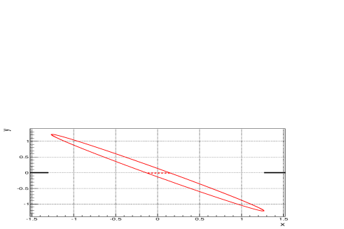
Figure 8: An illustration of constraints vs sensitivities: the red ellipse represents an experimentally allowed region of parameter space. Parameter $x$ is excluded outside the projection of the ellipse onto the axis (thick black line). The experiment is insensitive to $x$ inside the ellipse.

Three ways to relate low-energy experimental bounds to the coefficients of operators at a higher scale are:

1. to calculate the sensitivity of an experimental process to a particular operator coefficient. This is usually simple.

2. To express an experimental rate as a function of high-scale coefficients. This is slightly more difficult, because more coefficients are involved: each coefficient that contributes at the experimental scale will become a linear combination of high scale coefficients due the renormalisation group mixing.

3. To obtain constraints on coefficients at the high scale. This is more involved, because a sufficient number of experimental constraints must be combined, in order to obtain a finite allowed region in coefficient space (no “flat directions”). Then the allowed region must be projected onto the various axes, in order to obtain constraints.

The third option is the most useful, but beyond the scope of this work. Instead here, we partially follow the second option, as a contribution to the third: we consider experimental bounds on the dimension-six operators which are generated in RGE evolution by double-insertions of dimension-five operators that change lepton number. We aim to quote these bounds at $m_{W}$. The processes in question are LFV Higgs and $Z$ decays (which occur at the weak scale), and flavour-changing lepton decays at low energy (these bounds must be translated to the weak scale via the RGEs of QED and QCD). So we will not succeed in our aim of setting constraints on coefficients at $m_{W}$, because the low-energy experimental bounds depend on many coefficients at the weak scale, and we do not include enough experimental bounds.

In the following sections, we outline the calculations of the various rates, and summarise the experimental constraints on coefficients at $m_{W}$ in table E.1.

E.1 Rates and calculations

$\begin{array}[]{|c|c|c|}\hline\cr{\rm process}&{\rm BR}<&\frac{v^{2}}{\Lambda^{2}}|\sum C|<\\ \hline\cr Z\to e^{\pm}\mu^{\mp}&7.5\times 10^{-7}\cite[cite]{[\@@bibref{}{Aad:2014bca}{}{}]}&|C^{e\mu}_{H\ell(1)}+C^{e\mu}_{H\ell(3)}|<1.2\times 10^{-3}\\ Z\to\tau^{\pm}\mu^{\mp}&1.2\times 10^{-5}\cite[cite]{[\@@bibref{}{Abreu:1996mj}{}{}]}&|C^{\mu\tau}_{H\ell(1)}+C^{\mu\tau}_{H\ell(3)}|<4.6\times 10^{-3}\\ Z\to e^{\pm}\tau^{\mp}&9.8\times 10^{-6}\cite[cite]{[\@@bibref{}{Akers:1995gz}{}{}]}&|C^{e\tau}_{H\ell(1)}+C^{e\tau}_{H\ell(3)}|<4.1\times 10^{-3}\\ h\to e^{\pm}\mu^{\mp}&3.5\times 10^{-4}\cite[cite]{[\@@bibref{}{Khachatryan:2016rke}{}{}]}&|C^{\mu e}_{eH}|,|C^{e\mu}_{eH}|<2.5\times 10^{-4}\\ h\to\tau^{\pm}\mu^{\mp}&1.5\times 10^{-2}\cite[cite]{[\@@bibref{}{Khachatryan:2015kon}{}{}]}&|C^{\mu\tau}_{eH}|,|C^{\tau\mu}_{eH}|<1.6\times 10^{-3}\\ h\to e^{\pm}\tau^{\mp}&6.9\times 10^{-3}\cite[cite]{[\@@bibref{}{Khachatryan:2016rke}{}{}]}&|C^{e\tau}_{eH}|,|C^{\tau e}_{eH}|<1.1\times 10^{-3}\\ \hline\cr\tau\to ee\overline{e}&2.7\times 10^{-8}\cite[cite]{[\@@bibref{}{Hayasaka:2010np}{}{}]}&|{C}^{e\tau ee}_{\ell\ell}+{C}^{eee\tau}_{\ell\ell}+g_{L}^{e}[C^{e\tau}_{H\ell(1)}+C^{e\tau}_{H\ell(3)}]-\delta C_{penguin}^{e\tau}|<2.8\times 10^{-4}\\ &&|{C}^{e\tau ee}_{\ell e}+g_{R}^{e}[C^{e\tau}_{H\ell(1)}+C^{e\tau}_{H\ell(3)}]-\delta C_{penguin}^{e\tau}|<4.0\times 10^{-4}\\ \tau\to e\mu\overline{\mu}&2.7\times 10^{-8}\cite[cite]{[\@@bibref{}{Hayasaka:2010np}{}{}]}&|{C}^{e\tau\mu\mu}_{\ell\ell}+{C}^{\mu\mu e\tau}_{\ell\ell}+{C}^{e\mu\mu\tau}_{\ell\ell}+{C}^{\mu\tau e\mu}_{\ell\ell}+g_{L}^{e}[C^{e\tau}_{H\ell(1)}+C^{e\tau}_{H\ell(3)}]-\delta C_{penguin}^{e\tau}|<4.0\times 10^{-4}\\ &&|{C}^{e\tau\mu\mu}_{\ell e}+g_{R}^{e}[C^{\mu\tau}_{H\ell(1)}+C^{e\tau}_{H\ell(3)}]-\delta C_{penguin}^{e\tau}|<4.0\times 10^{-4}\\ \tau\to\mu e\overline{e}&1.8\times 10^{-8}\cite[cite]{[\@@bibref{}{Hayasaka:2010np}{}{}]}&|{C}^{\mu\tau ee}_{\ell\ell}+{C}^{ee\mu\tau}_{\ell\ell}{C}^{\mu ee\tau}_{\ell\ell}+{C}^{e\tau\mu e}_{\ell\ell}+g_{L}^{e}[C^{\mu\tau}_{H\ell(1)}+C^{\mu\tau}_{H\ell(3)}]-\delta C_{penguin}^{\mu\tau}|<3.2\times 10^{-4}\\ &&|{C}^{\mu\tau ee}_{\ell e}+g_{R}^{e}[C^{\mu\tau}_{H\ell(1)}+C^{\mu\tau}_{H\ell(3)}]-\delta C_{penguin}^{\mu\tau}|<3.2\times 10^{-4}\\ \tau\to\mu\mu\overline{\mu}&2.1\times 10^{-8}\cite[cite]{[\@@bibref{}{Hayasaka:2010np}{}{}]}&|{C}^{\mu\tau\mu\mu}_{\ell\ell}+{C}^{\mu\mu\mu\tau}_{\ell\ell}+g_{L}^{e}[C^{\mu\tau}_{H\ell(1)}+C^{\mu\tau}_{H\ell(3)}]-\delta C_{penguin}^{\mu\tau}|<2.5\times 10^{-4}\\ &&|{C}^{\mu\tau\mu\mu}_{\ell e}+g_{R}^{e}[C^{\mu\tau}_{H\ell(1)}+C^{\mu\tau}_{H\ell(3)}]-\delta C_{penguin}^{\mu\tau}|<3.5\times 10^{-4}\\ \tau\to ee\overline{\mu}&1.5\times 10^{-8}\cite[cite]{[\@@bibref{}{Hayasaka:2010np}{}{}]}&|{C}^{e\tau e\mu}_{\ell\ell}+{C}^{e\mu e\tau}_{\ell\ell}|<3.2\times 10^{-4}\\ \tau\to\mu\mu\overline{e}&1.7\times 10^{-8}\cite[cite]{[\@@bibref{}{Hayasaka:2010np}{}{}]}&|{C}^{\mu\tau\mu e}_{\ell\ell}+{C}^{\mu e\mu\tau}_{\ell\ell}|<3.2\times 10^{-4}\\ \mu\to 3e&1\times 10^{-12}\cite[cite]{[\@@bibref{}{Bellgardt:1987du}{}{}]}&|{C}^{e\mu ee}_{\ell\ell}+{C}^{eee\mu}_{\ell\ell}+g_{L}^{e}[C^{e\mu}_{H\ell(1)}+C^{e\mu}_{H\ell(3)}]-\delta C_{penguin}^{e\mu}|<7.1\times 10^{-7}\\ &&|{C}^{e\mu ee}_{\ell e}+g_{R}^{e}[C^{e\mu}_{H\ell(1)}+C^{e\mu}_{H\ell(3)}]-\delta C_{penguin}^{e\mu}|<1.0\times 10^{-6}\\ \tau\to e\gamma&3.3\times 10^{-8}\cite[cite]{[\@@bibref{}{Aubert:2009ag}{}{}]}&|C^{\tau e*}_{e\gamma}+\frac{e\alpha_{e}y_{t}}{8\pi^{3}y_{\mu}}C^{\tau e*}_{eH}+\frac{eg_{L}^{e}}{16\pi^{2}}C^{e\tau}_{He}|<7.3\times 10^{-6}\\ &&|C^{e\tau}_{e\gamma}+\frac{e\alpha_{e}y_{t}}{8\pi^{3}y_{\mu}}C^{e\tau}_{eH}+\frac{eg_{R}^{e}}{16\pi^{2}}[C^{e\tau}_{H\ell(1)}+C^{e\tau}_{H\ell(3)}]|<7.3\times 10^{-6}\\ \tau\to\mu\gamma&4.4\times 10^{-8}\cite[cite]{[\@@bibref{}{Aubert:2009ag,Hayasaka:2007vc}{}{}]}&|C^{\tau\mu*}_{e\gamma}+\frac{e\alpha_{e}y_{t}}{8\pi^{3}y_{\mu}}C^{\tau\mu*}_{eH}+\frac{eg_{L}^{e}}{16\pi^{2}}C^{\mu\tau}_{He}|<8.1\times 10^{-6}\\ &&|C^{\mu\tau}_{e\gamma}+\frac{e\alpha_{e}y_{t}}{8\pi^{3}y_{\mu}}C^{\mu\tau}_{eH}+\frac{eg_{R}^{e}}{16\pi^{2}}[C^{\mu\tau}_{H\ell(1)}+C^{\mu\tau}_{H\ell(3)}]|<8.1\times 10^{-6}\\ \mu\to e\gamma&4.2\times 10^{-13}\cite[cite]{[\@@bibref{}{TheMEG:2016wtm}{}{}]}&|C^{\mu e*}_{e\gamma}+\frac{e\alpha_{e}y_{t}}{8\pi^{3}y_{\mu}}C^{\mu e*}_{eH}+\frac{eg_{L}^{e}}{16\pi^{2}}C^{e\mu}_{He}|<1.05\times 10^{-8}\\ &&|C^{e\mu}_{e\gamma}+\frac{e\alpha_{e}y_{t}}{8\pi^{3}y_{\mu}}C^{e\mu}_{eH}+\frac{eg_{R}^{e}}{16\pi^{2}}[C^{e\mu}_{H\ell(1)}+C^{e\mu}_{H\ell(3)}]|<1.05\times 10^{-8}\\ \hline\cr\end{array}$ table Bound on operator coefficients of the SMEFT, evaluated at $m_{W}$, from the bounds listed in column 2 on the processes of column 1. The bounds on coefficients of hermitian operators (${\cal O}_{H\ell(1)}$, ${\cal O}_{H\ell(3)}$, ${\cal O}_{\ell\ell},{\cal O}_{\ell e}$) also apply to the conjugate coefficient. All the bounds apply to running coefficients evaluated at $m_{W}$, and are for $\Lambda=v\simeq m_{t}$. The combination of coefficients $C_{penguin}$ is defined in eqn(E.12) and before eqn (E.23), $\delta$ is defined after eqn (E.23), and $g_{R}^{e}=2s_{W}^{2}$, $g_{L}^{e}=-1+2s_{W}^{2}$.

E.1.1 $\bm{Z\to l_{\alpha}\bar{l}_{\beta}}$ decay

When the Higgs gets a vev, the “penguin” operators ${\cal O}_{H\ell(1)}$ and ${\cal O}_{H\ell(3)}$ generate a vertex involving the $Z$ and two charged leptons. If the flavour-changing $Z$-fermion vertex is written in a SM-like form : $-\overline{l_{\alpha}}Z^{\mu}\frac{g}{2c_{W}}\gamma_{\mu}(g_{V}-g_{A}\gamma_{5})l_{\beta}$, then

$$g_{V}=g_{A}=-(C_{H\ell(1)}+C_{H\ell(3)})\frac{v^{2}}{\Lambda^{2}}$$ (E.1)

(for $v\sim m_{t}$).

The branching ratio can be written

$$BR(Z\to l_{\alpha}\overline{l_{\beta}})=\frac{M_{Z}}{2.5{\rm GeV}}\frac{g^{2}}{48\pi c_{W}^{2}}(|g_{V}|^{2}+|g_{A}|^{2})$$ (E.2)

where 2.5 GeV is the $Z$ width in the SM. Since ${\cal O}_{H\ell(1)}$ and ${\cal O}_{H\ell(3)}$ are hermitian, the conjugate process $Z\to l_{\beta}\overline{l_{\alpha}}$ neccessarily occurs at the same rate, so the BR to the experimental final state is

$$BR(Z\to l^{\pm}_{\alpha}l^{\mp}_{\beta})=BR(Z\to l_{\alpha}\overline{l_{\beta}})+BR(Z\to l_{\beta}\overline{l_{\alpha}})=\frac{M_{Z}}{2.5{\rm GeV}}\frac{g^{2}}{12\pi c_{W}^{2}}|(C^{\alpha\beta}_{H\ell(1)}+C^{\alpha\beta}_{H\ell(3)}|^{2}\frac{v^{4}}{\Lambda^{4}}$$ (E.3)

and the bounds we obtain on the operator coefficients, evaluated at $\sim m_{W}$, are given in table E.1.

E.1.2 $\bm{h\to\ell_{\alpha}^{+}e_{\beta}^{-},e_{\alpha}^{+}\ell_{\beta}^{-}}$ decays

The flavour-changing Higgs decays occur via the non-hermitian operator ${\cal O}_{eH}$. When the Higgs has a vev, it induces the Feynman rules for a flavour-changing Higgs vertex with two fermions:

$$C^{\alpha\beta}_{eH}{\cal O}^{\alpha\beta}_{eH}\longrightarrow i\frac{3C^{\alpha\beta}_{eH}v^{2}}{\sqrt{2}\Lambda^{2}}P_{R}~{}~{}~{}~{}~{},~{}~{}~{}~{}~{}C^{\beta\alpha*}_{eH}{\cal O}^{\beta\alpha*}_{eH}\longrightarrow i\frac{3C^{\beta\alpha*}_{eH}v^{2}}{\sqrt{2}\Lambda^{2}}P_{L}\,.$$ (E.4)

We calculate the flavour-changing branching ratio by comparing to $BR(h\to b\bar{b})=0.575\pm 0.32$ (from the Appendix of the Higgs Working Group Report [35], for $m_{h}=125.1$ GeV), assuming the Feynman rule for $hb\bar{b}$ is $-\frac{i}{\sqrt{2}}y_{b}(m_{h})P_{L,R}$. We use a one-loop approximation [15] for the running $b$ mass

$$y_{b}(m_{h})v=m_{b}(m_{b})\left[\frac{\alpha(m_{h})}{\alpha(m_{b})}\right]^{\gamma_{m}^{(0)}/2\beta^{(0)}}\simeq 3.0~{}{\rm GeV}$$ (E.5)

where $\alpha(m_{h})\simeq 0.12,\alpha(m_{b})\simeq.23$,$\gamma_{m}^{(0)}=8$, $\beta^{(0)}=23/3$ and $m_{b}(m_{b})=4.2$ GeV.

The operator ${\cal O}_{eH}$ is not hermitian, but is always included in the Lagrangian $+\mathrm{h.c.}$. So $C^{e\mu}_{eH}{\cal O}^{e\mu}_{eH}+\mathrm{h.c.}$ will induce both $h\to e_{L}\overline{\mu_{R}}$ and $h\to\mu_{R}\overline{e_{L}}$ at the same rate:

$$\frac{BR(h\to\overline{e_{L}}\mu_{R})}{BR(h\to b\bar{b})}=\frac{9|C^{e\mu}_{eH}|^{2}v^{2}}{6y_{b}^{2}\Lambda^{4}}~{}~{}~{},$$ (E.6)

where downstairs there is a 3 for quark colour sums, and a 2 from the chiral projectors in the lepton decay. The experimental search sums the $e_{L}\overline{\mu_{R}}$ and $\mu_{R}\overline{e_{L}}$ final states, so we obtain

$$3v^{2}\frac{|C^{\alpha\beta}_{eH}|^{2}}{\Lambda^{2}}~{},~{}3v^{2}\frac{|C^{\beta\alpha}_{eH}|^{2}}{\Lambda^{2}}\leq y_{b}^{2}(m_{h})\frac{BR(h\to l_{\alpha}^{\pm}l_{\beta}^{\mp})}{BR(h\to b\bar{b})}$$ (E.7)

and the resulting contraints are given in table E.1.

E.1.3 Including the low energy decays

The flavour-changing $\tau$ and $\mu$ decays listed in table E.1 occur at energies $\sim m_{\mu},m_{\tau}$, so the decay rates are usually written in terms of the coefficients of dimension-six operators from the QCD$\times$QED invariant basis appropriate at low energies. These “low energy” coefficients, which we denote with a tilde $\widetilde{C}$, can be expressed in terms of SMEFT coefficients at $m_{W}$ by running them up to $m_{W}$, then matching the QCD$\times$QED-invariant operator basis onto the SMEFT. This was performed in [34] for $\mu\to e\gamma$, so we use the results of [34] for the radiative decays of section E.1.5. Reference [36] studied the Renormalisation Group evolution, below the weak scale, of the coefficients who mediate $\mu\to e\bar{e}e$ (as well those for as $\mu\to e\gamma$ and $\mu\!\to\!e~{}{\rm conversion}$); we use these results, combined with the weak-scale matching conditions of [34], for the discussion in section E.1.4 of three body leptonic decays of $\tau$s and $\mu$s. The minor differences between $\mu$ and $\tau$ decays are discussed in section E.1.4.

In the EFT below $m_{W}$, we use the basis of lepton-flavour-changing four-fermion operators introduced in [2, 34] for $\mu\leftrightarrow e$ flavour change . The operators and coefficients have as subscript their Lorentz structure ($V,S,T$) and the chiral projection operators of the two fermion bilinears, and the flavour indices of the four fermions as superscript. They wear tildes to distinguish them from the coefficients of SMEFT operators. We restrict to the dipole and vector operators, and neglect the scalars and tensors, which will turn out to be irrelevant for our study of LFV operators generated by double-insertions of LNV operators. So the four-fermion operator basis below $m_{W}$ is

$$\delta{\cal L}_{4f} = \sum_{\alpha\beta}\sum_{f}{\Big{[}}\widetilde{C}^{\alpha\beta ff}_{V,LL}(\overline{e_{\alpha}}\gamma^{\omega}P_{L}e_{\beta})(\overline{f}\gamma_{\omega}P_{L}f)+\widetilde{C}^{\alpha\beta ff}_{V,LR}(\overline{e_{\alpha}}\gamma^{\omega}P_{L}e_{\beta})(\overline{f}\gamma_{\omega}P_{R}f){\Big{]}}+h.c.$$ (E.8)

$$+\sum_{\alpha\beta\sigma\rho}{\Big{[}}\widetilde{C}^{\alpha\beta\sigma\rho}_{V,LL}(\overline{e_{\alpha}}\gamma^{\omega}P_{L}e_{\beta})(\overline{e_{\sigma}}\gamma_{\omega}P_{L}e_{\rho}){\Big{]}}+h.c.$$

where $\alpha\beta\in\{e\mu,\mu\tau,e\tau\}$, $f\in\{e,\mu,\tau,u,d,s,c,b\}$, and $\alpha\beta\sigma\rho\in\{e\tau e\mu,\mu\tau\mu e\}$. In addition, below $m_{W}$ we consider the photon dipole operators

$$\delta{\cal L}_{dipole}=\frac{m_{\beta}}{\Lambda^{2}}\left(C^{\alpha\beta}_{D,L}\overline{e^{\alpha}_{R}}\sigma^{\rho\sigma}e^{\beta}_{L}F_{\rho\sigma}+C^{\alpha\beta}_{D,R}\overline{e^{\alpha}_{L}}\sigma^{\rho\sigma}e^{\beta}_{R}F_{\rho\sigma}\right)+h.c.$$ (E.9)

because the SMEFT operators ${\cal O}_{Hl(1)}$, ${\cal O}_{Hl(3)}$ and ${\cal O}_{eH}$ match onto the dipole at $m_{W}$. The current bounds on $\mu\to e\gamma$, $\tau\to e\gamma$ and $\tau\to\mu\gamma$ will give the best sensitivity to the coefficients $C_{H\ell(1)}$, $C_{H\ell(3)}$ and $C_{eH}$ .

E.1.4 $\bm{\tau\to 3l}$ and $\bm{\mu\to 3e}$

The first step is to translate the experimental bounds into constraints on operator coefficients at the experimental scale. For the three-body leptonic decays of the $\tau$, it is convenient to define

$$\widetilde{BR}(\tau\to 3l)\equiv\frac{BR(\tau\to 3l)}{BR(\tau\to\mu\bar{\nu}\nu)}$$ (E.10)

(where $BR(\tau\to\mu\bar{\nu}\nu)=0.174$ [1]). Then $\widetilde{BR}(\tau\to 3l)$ can be directly compared to the branching ratio for $\mu\to 3e$ [2]:

$$BR(\mu\to e\bar{e}e)\frac{\Lambda^{2}}{v^{2}} = \frac{|\widetilde{C}_{S,LL}|^{2}+|\widetilde{C}_{S,RR}|^{2}}{8}+2|\widetilde{C}_{V,RR}+4e\widetilde{C}_{D,R}|^{2}+2|\widetilde{C}_{V,LL}+4e\widetilde{C}_{D,L}|^{2}$$

$$+(64\ln\frac{m_{\mu}}{m_{e}}-88)(|e\widetilde{C}_{D,R}|^{2}+|e\widetilde{C}_{D,L}|^{2})+|\widetilde{C}_{V,RL}+4e\widetilde{C}_{D,R}|^{2}+|\widetilde{C}_{V,LR}+4e\widetilde{C}_{D,L}|^{2}~{}~{},$$

where $2\sqrt{2}G_{F}=1/v^{2}$ and the generalisation to $\tau$ decays is straightforward, after accounting for 2s as we now discuss.

We calculate the decay rates in the approximation that all final state fermions are massless. Factors of 2 can arise when there are two identically-flavoured fermions in the final state: there will be 2 diagrams, and a factor of 1/2 in the final-state phase space. Then there are two cases:
a) if the identical fermions have the same chirality, there is constructive interference between the two diagrams (despite the fact that they have relative minus signs due to Fermi statistics), which doubles the rate. (This is consistent with $\mu\to 3e$ rate of Kuno and Okada [2] given above.)
b) if the fermions have different chirality, the interference is suppressed by final state masses (which are neglected), so the two for two diagrams cancels the 1/2 from phase space.

We set the dipole coefficients to zero, because they are better constrained by the radiative decays discussed in the next subsection (see table E.1). Then it is clear that each upper bounds on a three-body leptonic decay of the $\tau$ or $\mu$, implies six independent constraints on operator coefficients (evaluated at the experimental scale), those of interest to us are given in table E.1.4.

$\begin{array}[]{|c|c|c|}\hline\cr{\rm process}&{\rm\widetilde{BR}}<&\frac{v^{2}}{\Lambda^{2}}|C|<\\ \hline\cr\tau\to ee\overline{e}&1.6\times 10^{-7}&\widetilde{C}^{e\tau ee}_{V,LL}<2.8\times 10^{-4},\widetilde{C}^{e\tau ee}_{V,LR}<4\times 10^{-4}\\ \tau\to e\mu\overline{\mu}&1.6\times 10^{-7}&\widetilde{C}^{e\tau\mu\mu}_{V,LR},\widetilde{C}^{e\tau\mu\mu}_{V,LL}<4\times 10^{-4}\\ \tau\to\mu e\overline{e}&1.0\times 10^{-7}&\widetilde{C}^{\mu\tau ee}_{V,LR},\widetilde{C}^{\mu\tau ee}_{V,LL}<3.2\times 10^{-4}\\ \tau\to\mu\mu\overline{\mu}&1.2\times 10^{-7}&\widetilde{C}^{e\tau\mu\mu}_{V,LL}<2.5\times 10^{-4},\widetilde{C}^{e\tau\mu\mu}_{V,LR}<3.5\times 10^{-4}\\ \tau\to ee\overline{\mu}&8.6\times 10^{-8}&\widetilde{C}^{e\tau e\mu}_{V,LL}<3.2\times 10^{-4},\\ \tau\to\mu\mu\overline{e}&1.0\times 10^{-7}&\widetilde{C}^{\mu\tau\mu e}_{V,LL}<3.2\times 10^{-4}\\ \hline\cr\mu\to ee\overline{e}&1.0\times 10^{-12}&\widetilde{C}^{e\mu ee}_{V,LL}<7.1\times 10^{-7},\widetilde{C}^{e\mu ee}_{V,LR}<10^{-6}\\ \hline\cr\end{array}$ table Bounds on some operator coefficients from three-body lepton decays, evaluated at the experimental scale.

The operator coefficients $\widetilde{C}_{X}(m_{\tau})$ given in table E.1.4 can be expressed in terms of coefficients at $m_{W}$ using the one-loop RGEs [34, 36]:

$$\mu\frac{d}{d\mu}\widetilde{C}_{I}=\frac{\alpha_{e}}{4\pi}\widetilde{C}_{J}[\gamma_{e}]_{JI}\Rightarrow\widetilde{C}_{I}(m_{\tau})=\widetilde{C}_{J}(m_{W})[\delta_{JI}-\frac{\alpha_{e}}{4\pi}\ln\frac{m_{W}}{m_{\tau}}[\gamma_{e}]_{JI}+...]$$

where $[\gamma_{e}]$ is the one-loop anomalous dimension matrix of QED, $\ln\frac{m_{W}}{m_{\tau}}=3.85$, $\ln\frac{m_{W}}{m_{\mu}}=6.64$ and the approximate solution neglects the running of $\alpha_{e}$. The one-loop QED corrections involve photon exchange between two legs of the operator, which does not change the flavour or chiral indices, and also “penguin” diagrams, where two legs of the operator are closed in a loop, and a photon is attached, which turns into two external leg fermions. The “penguins” can change the chirality and flavour, and allow 2-lepton-2-quark operators to mix with the four-lepton operators. We therefore need a recipe for dealing with the quark-sector threshholds $m_{b}$, $m_{c}$ and $\Lambda_{QCD}$. We make the simplest approximation, which is to have a single low-energy threshhold at $m_{\tau}$, and run from $m_{W}\to m_{\tau}$ with five flavours of quark, and we use this low-energy scale also for the decays of the $\mu$. In this approximation, it is convenient to define the combination of operator coefficients

$$\widetilde{C}^{\alpha\beta}_{penguin} = -\frac{4N_{c}}{3}\sum_{q}Q_{q}(\widetilde{C}^{\alpha\beta qq}_{V,LL}+\widetilde{C}^{\alpha\beta qq}_{V,LR})+\frac{4}{3}\sum_{l}([1+\delta_{\alpha l}+\delta_{\beta l}]\widetilde{C}^{\alpha\beta ll}_{V,LL}+\widetilde{C}^{\alpha\beta ll}_{V,LR})$$ (E.12)

where $l\in\{e,\mu,\tau\}$, $q\in\{u,d,s,c,b\}$, and $Q_{q}$ is the electric charge of the quark. Then the coefficients constrained in table E.1.4 can be written

$$\widetilde{C}^{e\mu ee}_{V,LR}(m_{\tau}) = [1+12\frac{\alpha_{e}}{4\pi}\ln\frac{m_{W}}{m_{\tau}}]\widetilde{C}^{e\mu ee}_{V,LR}(m_{W})-\frac{\alpha_{e}}{4\pi}\ln\frac{m_{W}}{m_{\tau}}\widetilde{C}^{e\mu}_{penguin}(m_{W})$$ (E.13)

$$\widetilde{C}^{e\mu ee}_{V,LL}(m_{\tau}) = [1-12\frac{\alpha_{e}}{4\pi}\ln\frac{m_{W}}{m_{\tau}}]\widetilde{C}^{e\mu ee}_{V,LL}(m_{W})-\frac{\alpha_{e}}{4\pi}\ln\frac{m_{W}}{m_{\tau}}\widetilde{C}^{e\mu}_{penguin}(m_{W})$$ (E.14)

$$\widetilde{C}^{e\tau ll}_{V,LR}(m_{\tau}) = [1+12\frac{\alpha_{e}}{4\pi}\ln\frac{m_{W}}{m_{\tau}}]\widetilde{C}^{e\tau ll}_{V,LR}(m_{W})-\frac{\alpha_{e}}{4\pi}\ln\frac{m_{W}}{m_{\tau}}\widetilde{C}^{e\tau}_{penguin}(m_{W})$$ (E.15)

$$\widetilde{C}^{e\tau ll}_{V,LL}(m_{\tau}) = [1-12\frac{\alpha_{e}}{4\pi}\ln\frac{m_{W}}{m_{\tau}}]\widetilde{C}^{e\tau ll}_{V,LL}(m_{W})-\frac{\alpha_{e}}{4\pi}\ln\frac{m_{W}}{m_{\tau}}\widetilde{C}^{e\tau}_{penguin}(m_{W})$$ (E.16)

$$\widetilde{C}^{\mu\tau ll}_{V,LR}(m_{\tau}) = [1+12\frac{\alpha_{e}}{4\pi}\ln\frac{m_{W}}{m_{\tau}}]\widetilde{C}^{\mu\tau ll}_{V,LR}(m_{W})-\frac{\alpha_{e}}{4\pi}\ln\frac{m_{W}}{m_{\tau}}\widetilde{C}^{\mu\tau}_{penguin}(m_{W})$$ (E.17)

$$\widetilde{C}^{\mu\tau ll}_{V,LL}(m_{\tau}) = [1-12\frac{\alpha_{e}}{4\pi}\ln\frac{m_{W}}{m_{\tau}}]\widetilde{C}^{\mu\tau ll}_{V,LL}(m_{W})-\frac{\alpha_{e}}{4\pi}\ln\frac{m_{W}}{m_{\tau}}\widetilde{C}^{\mu\tau}_{penguin}(m_{W})$$ (E.18)

$$\widetilde{C}^{\mu\tau\mu e}_{V,LL}(m_{\tau}) = [1-12\frac{\alpha_{e}}{4\pi}\ln\frac{m_{W}}{m_{\tau}}]\widetilde{C}^{\mu\tau\mu e}_{V,LL}(m_{W})$$ (E.19)

$$\widetilde{C}^{e\tau e\mu}_{V,LL}(m_{\tau}) = [1-12\frac{\alpha_{e}}{4\pi}\ln\frac{m_{W}}{m_{\tau}}]\widetilde{C}^{e\tau e\mu}_{V,LL}(m_{W})\,.$$ (E.20)

Finally, the combinations of coefficients that are constrained by data can be matched at $m_{W}$ onto coefficients of SMEFT operators [34]:

$$\widetilde{C}^{e\tau e\mu}_{V,LL}(m_{W}) = {C}^{e\tau e\mu}_{\ell\ell}(m_{W})+{C}^{e\mu e\tau}_{\ell\ell}(m_{W})$$ (E.21)

$$\widetilde{C}^{\mu\tau\mu e}_{V,LL}(m_{W}) = {C}^{\mu\tau\mu e}_{\ell\ell}(m_{W})+{C}^{\mu e\mu\tau}_{\ell\ell}(m_{W})$$

$$\widetilde{C}^{\mu\tau ee}_{V,LL}(m_{W}) = {C}^{\mu\tau ee}_{\ell\ell}(m_{W})+{C}^{ee\mu\tau}_{\ell\ell}(m_{W})+{C}^{\mu ee\tau}_{\ell\ell}(m_{W})+{C}^{e\tau\mu e}_{\ell\ell}(m_{W})+g_{L}^{e}[C^{\mu\tau}_{H\ell(1)}(m_{W})+C^{\mu\tau}_{H\ell(3)}(m_{W})]$$

$$\widetilde{C}^{\mu\tau\mu\mu}_{V,LL}(m_{W}) = {C}^{\mu\tau\mu\mu}_{\ell\ell}(m_{W})+{C}^{\mu\mu\mu\tau}_{\ell\ell}(m_{W})+g_{L}^{e}[C^{\mu\tau}_{H\ell(1)}(m_{W})+C^{\mu\tau}_{H\ell(3)}(m_{W})]$$

$$\widetilde{C}^{\mu\tau ll}_{V,LR}(m_{W}) = {C}^{\mu\tau ll}_{\ell e}(m_{W})+g_{R}^{e}[C^{\mu\tau}_{H\ell(1)}(m_{W})+C^{\mu\tau}_{H\ell(3)}(m_{W})]$$

$$\widetilde{C}^{e\tau\mu\mu}_{V,LL}(m_{W}) = {C}^{e\tau\mu\mu}_{\ell\ell}(m_{W})+{C}^{\mu\mu e\tau}_{\ell\ell}(m_{W})+{C}^{e\mu\mu\tau}_{\ell\ell}(m_{W})+{C}^{\mu\tau e\mu}_{\ell\ell}(m_{W})+g_{L}^{e}[C^{e\tau}_{H\ell(1)}(m_{W})+C^{e\tau}_{H\ell(3)}(m_{W})]$$

$$\widetilde{C}^{e\tau ee}_{V,LL}(m_{W}) = {C}^{e\tau ee}_{\ell\ell}(m_{W})+{C}^{eee\tau}_{\ell\ell}(m_{W})+g_{L}^{e}[C^{e\tau}_{H\ell(1)}(m_{W})+C^{e\tau}_{H\ell(3)}(m_{W})]$$

$$\widetilde{C}^{e\tau ll}_{V,LR}(m_{W}) = {C}^{e\tau ll}_{\ell e}(m_{W})+g_{R}^{e}[C^{e\tau}_{H\ell(1)}(m_{W})+C^{e\tau}_{H\ell(3)}(m_{W})]$$

$$\widetilde{C}^{e\mu ee}_{V,LL}(m_{W}) = {C}^{e\mu ee}_{\ell\ell}(m_{W})+{C}^{eee\mu}_{\ell\ell}(m_{W})+g_{L}^{e}[C^{e\mu}_{H\ell(1)}(m_{W})+C^{e\mu}_{H\ell(3)}(m_{W})]$$

$$\widetilde{C}^{e\mu ee}_{V,LR}(m_{W}) = {C}^{e\mu ee}_{\ell e}(m_{W})+g_{R}^{e}[C^{e\mu}_{H\ell(1)}(m_{W})+C^{e\mu}_{H\ell(3)}(m_{W})]$$

where $l\in\{e,\mu\}$ in the above equations, and $g_{R}^{e}=2\sin^{2}\theta_{W}$, $g_{L}^{e}=-1+2\sin^{2}\theta_{W}$. In order to match the “penguin” coefficient of eqn (E.12) onto coefficients of the SMEFT, matching conditions for operators with a quark bilinear are also required:

$$\widetilde{C}^{\alpha\beta uu}_{V,LL}(m_{W}) = {C}^{\alpha\beta uu}_{\ell q(1)}(m_{W})-{C}^{\alpha\beta uu}_{\ell q(3)}(m_{W})+g_{L}^{u}[C^{\alpha\beta}_{H\ell(1)}(m_{W})+C^{\alpha\beta}_{H\ell(3)}(m_{W})]$$

$$\widetilde{C}^{\alpha\beta dd}_{V,LL}(m_{W}) = {C}^{\alpha\beta dd}_{\ell q(1)}(m_{W})+{C}^{\alpha\beta dd}_{\ell q(3)}(m_{W})+g_{L}^{d}[C^{\alpha\beta}_{H\ell(1)}(m_{W})+C^{\alpha\beta}_{H\ell(3)}(m_{W})]$$

$$\widetilde{C}^{\alpha\beta uu}_{V,LR}(m_{W}) = {C}^{\alpha\beta uu}_{\ell u}(m_{W})+g_{R}^{u}[C^{\alpha\beta}_{H\ell(1)}(m_{W})+C^{\alpha\beta}_{H\ell(3)}(m_{W})]$$

$$\widetilde{C}^{\alpha\beta dd}_{V,LR}(m_{W}) = {C}^{\alpha\beta dd}_{\ell d}(m_{W})+g_{R}^{d}[C^{\alpha\beta}_{H\ell(1)}(m_{W})+C^{\alpha\beta}_{H\ell(3)}(m_{W})]$$ (E.22)

where $\alpha\beta\in\{\mu\tau,e\tau,e\mu\}$, $g_{L}^{u}=1-\frac{4}{3}\sin^{2}\theta_{W}$, $g_{R}^{u}=-\frac{4}{3}\sin^{2}\theta_{W}$, $g_{L}^{d}=-1+\frac{2}{3}\sin^{2}\theta_{W}$ and, $g_{R}^{d}=\frac{2}{3}\sin^{2}\theta_{W}$. Combining the definition (E.12) with the matching conditions of eqn (E.22) allows the definition of a combination of SMEFT coefficients $C_{penguin}^{\alpha\beta}(m_{W})$. Then the experimental constraint on, for instance $\widetilde{C}^{e\tau\mu\mu}_{V,LL}(m_{\tau})$, gives

$${\Big{|}}{\Big{[}}1-12\delta{\Big{]}}{\Big{[}}{C}^{e\tau\mu\mu}_{\ell\ell}+{C}^{\mu\mu e\tau}_{\ell\ell}+{C}^{e\mu\mu\tau}_{\ell\ell}+{C}^{\mu\tau e\mu}_{\ell\ell}+g_{L}^{e}[C^{e\tau}_{H\ell(1)}+C^{e\tau}_{H\ell(3)}]{\Big{]}}-\delta C_{penguin}^{\alpha\beta}{\Big{|}}<4\times 10^{-4}$$ (E.23)

where all the coefficients are evaluated at $m_{W}$, and $\delta=\frac{\alpha_{e}}{4\pi}\ln\frac{m_{W}}{m_{\tau}}\sim 1/400$. This and other constraints from 3-body $\tau$ decays are given in table E.1, where for compactness, $[1\pm 12\delta]$ is approximated as 1.

E.1.5 $\bm{l_{\beta}\to l_{\alpha}\gamma}$

The radiative decays $l_{\beta}\to l_{\alpha}\gamma$ provide some of the most restrictive bounds on lepton flavour violation. The branching ratio at $m_{\beta}$ can be written

$$\widetilde{BR}(l_{\beta}\to l_{\alpha}\gamma)\equiv\frac{BR(l_{\beta}\to l_{\alpha}\gamma)}{BR(l_{\beta}\to l_{\alpha}\bar{\nu}\nu)}=384\pi^{2}\frac{v^{2}}{\Lambda^{2}}(|C^{\alpha\beta}_{D,L}|^{2}+|C^{\alpha\beta}_{D,R}|^{2})\leq\left\{\begin{array}[]{ll}4.2\times 10^{-13}&\mu\to e\gamma\\ 2.0\times 10^{-7}&\tau\to e\gamma\\ 2.5\times 10^{-7}&\tau\to\mu\gamma\\ \end{array}\right.$$ (E.24)

where the low energy dipole operators are added to the Lagrangian as in eqn (E.9).

The dipole coefficients evaluated at the experimental scale can be expressed in terms of SMEFT coefficients at the weak scale as [34]

$$C^{\alpha\beta}_{D,L}(m_{\tau}) = C^{\beta\alpha*}_{e\gamma}(m_{W})+\frac{e\alpha_{e}y_{t}}{8\pi^{3}y_{\mu}}C^{\beta\alpha*}_{eH}(m_{W})+\frac{eg_{L}^{e}}{16\pi^{2}}C^{\alpha\beta}_{He}(m_{W})+...$$ (E.25)

$$C^{\alpha\beta}_{D,R}(m_{\tau}) = C^{\alpha\beta}_{e\gamma}(m_{W})+\frac{e\alpha_{e}y_{t}}{8\pi^{3}y_{\mu}}C^{\alpha\beta}_{eH}(m_{W})+\frac{eg_{R}^{e}}{16\pi^{2}}[C^{\alpha\beta}_{H\ell(1)}(m_{W})+C^{\alpha\beta}_{H\ell(3)}(m_{W})+...$$ (E.26)

where the contributions of scalar and tensor four-fermion operators were neglected, $g_{R}^{e}$ and $g_{L}^{e}$ are defined after eqn(E.21), and

$$C^{\alpha\beta}_{e\gamma}=c_{W}C^{\alpha\beta}_{eB}-s_{W}C^{\alpha\beta}_{eW}~{}~{}.$$ (E.27)

Appendix F Comparison with the Literature

The standard model calculation has been performed in Reference [21] in a different operator basis. We disagree with their final results even after transforming our results to their basis. To do this we specify our basis

$$\tilde{\mathcal{O}}=\left(\mathcal{O}_{H\ell(1)},\mathcal{O}_{H\ell(3)},\mathcal{O}_{eH},\mathcal{O}_{eH}^{\dagger},\mathcal{O}_{v(1)},\mathcal{O}_{v(1)}^{\dagger},\mathcal{O}_{v(3)},\mathcal{O}_{v(3)}^{\dagger}\right)^{T}\,,$$ (F.1)

and the one used in Reference [21]

$$\tilde{Q}=\left(Q_{\phi\ell}^{(-)},Q_{\phi\ell}^{(+)},Q_{e\phi},Q_{e\phi}^{\dagger},\mathcal{O}_{v(1)},\mathcal{O}_{v(1)}^{\dagger},\mathcal{O}_{v(3)},\mathcal{O}_{v(3)}^{\dagger}\right)^{T}\,,$$ (F.2)

where the additional operators are defined as

$$Q_{\phi\ell}^{(-)} = \frac{i}{2}\left[(H^{\dagger}D_{\mu}H)(\bar{\ell}\gamma^{\mu}\ell)-(H^{\dagger}D_{\mu}^{a}H)(\bar{\ell}\tau^{a}\gamma^{\mu}\ell)\right]$$ (F.3)

$$Q_{\phi\ell}^{(+)} = \frac{i}{2}\left[(H^{\dagger}D_{\mu}H)(\bar{\ell}\gamma^{\mu}\ell)+(H^{\dagger}D_{\mu}^{a}H)(\bar{\ell}\tau^{a}\gamma^{\mu}\ell)\right]$$ (F.4)

$$Q_{e\phi} = \mathcal{O}_{eH}\,.$$ (F.5)

Here we drop the generation indices and note that the operators $Q_{\phi\ell}^{(-)}$ and $Q_{\phi\ell}^{(+)}$ are not hermitian. For this reason we treat the operator $\mathcal{O}_{eH}$ and the EOM-vanishing operators independent from their hermitian conjugate in our basis transformation. Writing the resulting linear transformation as

$$\tilde{\mathcal{O}}=\hat{R}\tilde{Q}\,,$$

only the first two rows of $\hat{R}$ have entries that are not proportional to an identity transformation. These two rows are determined by the following linear transformation:

$$\begin{pmatrix}\mathcal{O}_{H\ell(1)}\\ \mathcal{O}_{H\ell(3)}\end{pmatrix}=\begin{pmatrix}2&2&Y&-Y^{\dagger}&1&-1&0&0\\ -2&2&Y&-Y^{\dagger}&0&0&1&-1\\ \end{pmatrix}\tilde{O}\,.$$ (F.6)

The Wilson coefficients and renormalisation constants will consequently fulfil our hermiticity conditions in our basis, but not necessarily in the basis of Reference [21]. The counterterms of the Wilson coefficients transform in the same way as the respective Wilson coefficients under our change of basis, i.e. as

$$\delta\tilde{c}=\hat{R}^{T}\delta\tilde{C}\,,$$

where $\delta\tilde{C}=(16\pi^{2})\epsilon\vec{C}\tilde{Z}\vec{C}^{\dagger}$ represent the counterterms multiplied with $(16\pi^{2})\epsilon$, while $\delta\tilde{c}$ correspond to the analogous expression in the $\tilde{Q}$ basis.

Using the counterterms presented in Equations (3.2), (3.3) and (3.6), and the results of (F.8) we obtain

$$\delta\tilde{c}=\left(-\frac{5}{2}\big{[}C_{5}C_{5}^{*}\big{]},-\frac{1}{2}\big{[}C_{5}C_{5}^{*}\big{]},\frac{1}{2}\big{[}C_{5}C_{5}^{*}Y\big{]},\big{[}Y^{\dagger}C_{5}^{*}C_{5}\big{]}\right)^{T}\,,$$ (F.7)

which fulfil the hermiticity condition of the overall Lagrangian, even though this is not immediately apparent due to the choice of basis. These results are in disagreement with the final results quoted in Reference [21]. Yet using the results quoted in the individual diagrams in Appendix B of Reference [21] we find agreement with the expression of eqn (F.7) apart from a global minus sign, which suggests that a different projection was performed. We explicitly checked that the diagrams given in Appendices B.1, B.3 and B.4 of their calculation have the opposite sign compared with our calculation, while we agree with their lepton conserving contribution presented in Appendix B.2. Following the explanations of the calculation it appears that part (the $\delta\delta$ part) of the diagram evaluated in Appendix B.1 of Reference [21] is projected onto an operator basis where the operators $Q_{\phi\ell}^{(\pm)}$ are replaced by $Q_{\phi\ell}^{(\pm)\prime}=Q_{\phi\ell}^{(\pm)}+(Q_{\phi\ell}^{(\pm)})^{\dagger}$, while another part (the $\epsilon\epsilon$ part) is projected onto the basis presented in eqn (F.2).

Transforming now to the primed basis, where the hermitian conjugate is added to the first two operators of eqn (F.2) we find that the non-trivial transformation matrix involves only the first two elements of our and the primed basis. Writing explicitly

$$\begin{pmatrix}\mathcal{O}_{H\ell(1)}\\ \mathcal{O}_{H\ell(3)}\end{pmatrix}=\begin{pmatrix}1&1\\ -1&1\\ \end{pmatrix}\begin{pmatrix}\mathcal{O}_{H\ell}^{(-)\prime}\\ \mathcal{O}_{H\ell}^{(+)\prime}\end{pmatrix}\,,$$ (F.8)

we find

$$\delta\tilde{c}^{\prime}=\left(-\frac{5}{4}\big{[}C_{5}C_{5}^{*}\big{]},-\frac{1}{4}\big{[}C_{5}C_{5}^{*}\big{]},\frac{3}{4}\big{[}C_{5}C_{5}^{*}Y\big{]},\frac{3}{4}\big{[}Y^{\dagger}C_{5}^{*}C_{5}\big{]}\right)^{T}\,.$$ (F.9)

Again, this result does not agree with Reference [21]. Finally, note that projecting the results quoted for the individual diagrams in Appendix B of Reference [21], except the $\varepsilon\varepsilon$ part, would give

$$\delta\tilde{c}^{\prime}_{\mathrm{not}\;\varepsilon\varepsilon}=\left(+\frac{1}{4}\big{[}C_{5}C_{5}^{*}\big{]},+\frac{1}{4}\big{[}C_{5}C_{5}^{*}\big{]},-\frac{3}{4}\big{[}C_{5}C_{5}^{*}Y\big{]},-\frac{3}{4}\big{[}Y^{\dagger}C_{5}^{*}C_{5}\big{]}\right)^{T}\,,$$ (F.10)

while projecting only the $\varepsilon\varepsilon$ part on the non-hermitian basis yields $\delta\tilde{c}_{\varepsilon\varepsilon}=\left(+2\big{[}C_{5}C_{5}^{*}\big{]},0,0,0\right)^{T}$. Summing these two terms would reproduce the results of Reference [21].

Appendix G Flavour Conserving Contribution

Even though the diagram in figure 2 cannot induce lepton flavour violation it contributes to the renormalisation of $\mathcal{O}_{eH}$ and the corresponding operators that involve quarks. We also explicitly checked that the diagrams that involve six external Higgses vanish after summing over them. Denoting the trace over the product of the two dimension-five Wilson coefficients by $\mathrm{Tr}[C_{5}C_{5}^{*}]$ we find

$$\begin{split}(\vec{C}[\tilde{Z}]\vec{C}^{\dagger})^{\beta\alpha}_{eH}&=-\frac{1}{16\pi^{2}\epsilon}\mathrm{Tr}[C_{5}C_{5}^{*}][Y_{e}]_{\beta\alpha}\,,\\ (\vec{C}[\tilde{Z}]\vec{C}^{\dagger})^{\beta\alpha}_{uH}&=-\frac{1}{16\pi^{2}\epsilon}\mathrm{Tr}[C_{5}C_{5}^{*}][Y_{u}]_{\beta\alpha}\,,\\ (\vec{C}[\tilde{Z}]\vec{C}^{\dagger})^{\beta\alpha}_{dH}&=-\frac{1}{16\pi^{2}\epsilon}\mathrm{Tr}[C_{5}C_{5}^{*}][Y_{d}]_{\beta\alpha}\,,\end{split}$$ (G.1)

where $Y_{u}$ and $Y_{d}$ are defined as $\Gamma_{u}$ and $\Gamma_{d}$ of reference [20]. In addition we also generate the following mixing into operators that only comprise Higgs and gauge fields and write

$$\begin{split}(\vec{C}[\tilde{Z}]\vec{C}^{\dagger})_{H}&=-2\frac{1}{16\pi^{2}\epsilon}\mathrm{Tr}[C_{5}C_{5}^{*}]\lambda\,,\\ (\vec{C}[\tilde{Z}]\vec{C}^{\dagger})_{HD}&=-2\frac{1}{16\pi^{2}\epsilon}\mathrm{Tr}[C_{5}C_{5}^{*}]\,,\\ (\vec{C}[\tilde{Z}]\vec{C}^{\dagger})_{H\Box}&=-\frac{1}{16\pi^{2}\epsilon}\mathrm{Tr}[C_{5}C_{5}^{*}]\,,\end{split}$$ (G.2)

where the additional operators are defined as:

$$\begin{split}\mathcal{O}_{dH}^{\alpha\beta}&=(H^{\dagger}H)\overline{q}_{\alpha}Hd_{\beta}\\ \mathcal{O}_{uH}^{\alpha\beta}&=(H^{\dagger}H)\overline{q}_{\alpha}\epsilon H^{*}u_{\beta}\\ \mathcal{O}_{H}&=\frac{1}{2}\left(H^{\dagger}H\right)^{3}\\ \mathcal{O}_{HD}&=\frac{1}{2}\left(H^{\dagger}D^{\mu}H\right)^{*}\left(H^{\dagger}D_{\mu}H\right)\\ \mathcal{O}_{H\Box}&=\frac{1}{2}\left(H^{\dagger}H\right)\Box\left(H^{\dagger}H\right)\,.\end{split}$$ (G.3)

References

• [1] “2017 Review of Particle Physics”, C. Patrignani et al. (Particle Data Group), Chin. Phys. C, 40, 100001 (2016) and 2017 update.
• [2] Y. Kuno and Y. Okada, “Muon decay and physics beyond the standard model,” Rev. Mod. Phys.  73 (2001) 151 [arXiv:hep-ph/9909265].
• [3] A. M. Baldini et al. [MEG Collaboration], “Search for the lepton flavour violating decay $\mu^{+}\rightarrow e^{+}\gamma$ with the full dataset of the MEG experiment,” Eur. Phys. J. C 76 (2016) no.8, 434 [arXiv:1605.05081 [hep-ex]].
• [4] G. Aad et al. [ATLAS Collaboration], “Search for the lepton flavor violating decay $Z\to e\mu$ in $pp$ collisions at $\sqrt{s}$ TeV with the ATLAS detector,” Phys. Rev. D 90 (2014) no.7, 072010 [arXiv:1408.5774 [hep-ex]].
• [5] P. Abreu et al. [DELPHI Collaboration], “Search for lepton flavor number violating Z0 decays,” Z. Phys. C 73 (1997) 243.
• [6] R. Akers et al. [OPAL Collaboration], “A Search for lepton flavor violating Z0 decays,” Z. Phys. C 67 (1995) 555.
• [7] V. Khachatryan et al. [CMS Collaboration], “Search for lepton flavour violating decays of the Higgs boson to $e\tau$ and $e\mu$ in proton–proton collisions at $\sqrt{s}=$ 8 TeV,” Phys. Lett. B 763 (2016) 472 [arXiv:1607.03561 [hep-ex]].
• [8] V. Khachatryan et al. [CMS Collaboration], “Search for Lepton-Flavour-Violating Decays of the Higgs Boson,” Phys. Lett. B 749 (2015) 337 [arXiv:1502.07400 [hep-ex]].
• [9] K. Hayasaka et al., “Search for Lepton Flavor Violating Tau Decays into Three Leptons with 719 Million Produced Tau+Tau- Pairs,” Phys. Lett. B 687 (2010) 139 [arXiv:1001.3221 [hep-ex]].
• [10] U. Bellgardt et al. [SINDRUM Collaboration], “Search for the Decay $\mu^{+}\to e^{+}e^{+}e^{-}$,” Nucl. Phys. B 299 (1988) 1.
• [11] B. Aubert et al. [BaBar Collaboration], “Searches for Lepton Flavor Violation in the Decays tau+- to e+- gamma and tau+- to mu+- gamma,” Phys. Rev. Lett.  104 (2010) 021802 [arXiv:0908.2381 [hep-ex]].
• [12] K. Hayasaka et al. [Belle Collaboration], “New Search for $\tau\to\mu\gamma$ and $\tau\to e\gamma$ Decays at Belle,” Phys. Lett. B 666 (2008) 16 [arXiv:0705.0650 [hep-ex]].
• [13] J. D. Vergados, H. Ejiri and F. Simkovic, “Theory of Neutrinoless Double Beta Decay,” Rept. Prog. Phys.  75 (2012) 106301 [arXiv:1205.0649 [hep-ph]]. S. M. Bilenky and C. Giunti, “Neutrinoless Double-Beta Decay: a Probe of Physics Beyond the Standard Model,” Int. J. Mod. Phys. A 30 (2015) no.04n05, 1530001 [arXiv:1411.4791 [hep-ph]].
• [14] H. Georgi, “Effective field theory,” Ann. Rev. Nucl. Part. Sci.  43 (1993) 209-252.
H. Georgi, “On-shell effective field theory,” Nucl. Phys.  B361 (1991) 339-350.
• [15] A. J. Buras, “Weak Hamiltonian, CP violation and rare decays,” [arXiv:hep-ph/9806471]. G. Buchalla, A. J. Buras and M. E. Lautenbacher, “Weak decays beyond leading logarithms,” Rev. Mod. Phys.  68 (1996) 1125 [arXiv:hep-ph/9512380].
• [16] K. S. Babu, C. N. Leung and J. T. Pantaleone, “Renormalization of the neutrino mass operator,” Phys. Lett. B 319 (1993) 191 [arXiv:hep-ph/9309223]. P. H. Chankowski and Z. Pluciennik, “Renormalization group equations for seesaw neutrino masses,” Phys. Lett. B 316 (1993) 312 [arXiv:hep-ph/9306333]. S. Antusch, M. Drees, J. Kersten, M. Lindner and M. Ratz, “Neutrino mass operator renormalization revisited,” Phys. Lett. B 519 (2001) 238 [arXiv:hep-ph/0108005].
• [17] S. Antusch, M. Drees, J. Kersten, M. Lindner and M. Ratz, Phys. Lett. B 525 (2002) 130 [arXiv:hep-ph/0110366].
• [18] W. Grimus and L. Lavoura, Eur. Phys. J. C 39 (2005) 219 [arXiv:hep-ph/0409231].
• [19] R. Alonso, E. E. Jenkins, A. V. Manohar and M. Trott, “Renormalization Group Evolution of the Standard Model Dimension Six Operators III: Gauge Coupling Dependence and Phenomenology,” JHEP 1404 (2014) 159 [arXiv:1312.2014 [hep-ph]]. E. E. Jenkins, A. V. Manohar and M. Trott, “Renormalization Group Evolution of the Standard Model Dimension Six Operators II: Yukawa Dependence,” JHEP 1401 (2014) 035 [arXiv:1310.4838 [hep-ph]]. E. E. Jenkins, A. V. Manohar and M. Trott, “Renormalization Group Evolution of the Standard Model Dimension Six Operators I: Formalism and lambda Dependence,” JHEP 1310 (2013) 087 [arXiv:1308.2627 [hep-ph]].
• [20] B. Grzadkowski, M. Iskrzynski, M. Misiak and J. Rosiek, “Dimension-Six Terms in the Standard Model Lagrangian,” JHEP 1010 (2010) 085 [arXiv:1008.4884 [hep-ph]].
• [21] A. Broncano, M. B. Gavela and E. E. Jenkins, “Renormalization of lepton mixing for Majorana neutrinos,” Nucl. Phys. B 705 (2005) 269 [arXiv:hep-ph/0406019].
• [22] W. Buchmuller and D. Wyler, “Effective Lagrangian Analysis of New Interactions and Flavor Conservation,” Nucl. Phys. B 268, 621 (1986).
• [23] A. Djouadi, “The Anatomy of electro-weak symmetry breaking. II. The Higgs bosons in the minimal supersymmetric model,” Phys. Rept.  459 (2008) 1 [arXiv:hep-ph/0503173]. G. C. Branco, P. M. Ferreira, L. Lavoura, M. N. Rebelo, M. Sher and J. P. Silva, “Theory and phenomenology of two-Higgs-doublet models,” Phys. Rept.  516 (2012) 1 [arXiv:1106.0034 [hep-ph]].
• [24] S. Weinberg, Phys. Rev. Lett. 43 (1979) 1566.
• [25] A. Denner, H. Eck, O. Hahn and J. Kublbeck, “Feynman rules for fermion number violating interactions,” Nucl. Phys. B 387 (1992) 467.
• [26] N. G. Deshpande and E. Ma, Phys. Rev. D 18 (1978) 2574.
• [27] E. Ma, Phys. Rev. D 73 (2006) 077301 [arXiv:hep-ph/0601225].
• [28] R. Barbieri, L. J. Hall and V. S. Rychkov, Phys. Rev. D 74 (2006) 015007 [arXiv:hep-ph/0603188].
• [29] A. Belyaev, G. Cacciapaglia, I. P. Ivanov, F. Rojas-Abatte and M. Thomas, Phys. Rev. D 97 (2018) no.3, 035011 [arXiv:1612.00511 [hep-ph]].
• [30] S. Davidson and H. E. Haber, “Basis-independent methods for the two-Higgs-doublet model,” Phys. Rev. D 72 (2005) 035004 Erratum: [Phys. Rev. D 72 (2005) 099902] [arXiv:hep-ph/0504050].
• [31] S. Herrlich and U. Nierste, “Evanescent operators, scheme dependences and double insertions,” Nucl. Phys. B 455 (1995) 39 [arXiv:hep-ph/9412375].
• [32] M. Gorbahn, S. Jager, U. Nierste and S. Trine, Phys. Rev. D 84 (2011) 034030 [arXiv:0901.2065 [hep-ph]].
• [33] M. E. Peskin and D. V. Schroeder, “An Introduction to quantum field theory,” Westview Press, 1995, ISBN 978-0-201-50397-5.
• [34] S. Davidson, Eur. Phys. J. C 76 (2016) no.7, 370 [arXiv:1601.07166 [hep-ph]].
• [35] S. Heinemeyer et al. [LHC Higgs Cross Section Working Group], “Handbook of LHC Higgs Cross Sections: 3. Higgs Properties,” [arXiv:1307.1347 [hep-ph]].
• [36] A. Crivellin, S. Davidson, G. M. Pruna and A. Signer, “Renormalisation-group improved analysis of $\mu\to e$ processes in a systematic effective-field-theory approach,” JHEP 1705 (2017) 117 [arXiv:1702.03020 [hep-ph]].