Phase structures emerging from holography with
Einstein gravity - dilaton models at finite temperature

Abstract

Asymptotic AdS Riemann space-times in five dimensions with a black brane (horizon) sourced by a fully back-reacted scalar field (dilaton) offer – via the holographic dictionary – various options for the thermodynamics of the flat four-dimensional boundary theory, uncovering Hawking-Page, first-order and second-order phase transitions up to a cross-over or featureless behavior. The relation of these phase structures to the dilaton potential is clarified and illustrating examples are presented. Having in mind applications to QCD we study probe vector mesons with the goal to figure out conditions for forming Regge type series of radial excitations and address the issue of meson melting.

I Introduction

The advent of the insight into AdS/CFT correspondence maldacena ; witten ; gubser offered the option of having an alternative access to strongly coupled systems, e.g. to various facets of QCD in the non-pertubative regime, for instance. Phenomenologically interesting problems, e.g. the hadron spectrum or properties of the quark-gluon plasma, become treatable within a framework called holographic approaches. Most desirably would be to have a holographic QCD dual at our disposal, from which statements on QCD-related quantities can be derived in a unique manner. However, such a dual is presently not available dual ; dual2 ; dual3 ; KKSS . Therefore, in practice, field-theory quantities in a five dimensional asymptotic Anti-de Sitter (AdS) are often related to observables (or expectation values of operators) in four dimensional Minkowski space-time in the spirit of the field-operator duality (dictionary , see also §5.3 in erdmenger , §10.3 in nastase , for instance). Top-down approaches attempt to use input from string theory constructions – or elements thereof. These are to be contrasted with bottom-up approaches which aim at starting with an appropriate model on the field-theory side to mimic certain selected features of the boundary theory side, with the latter being connected to the quantum field theory in Minkowski space, while the former includes the dynamics in the bulk.
Besides early emphasis on accessing principal features of strongly coupled systems with many extensions to higher or lower dimensions than mentioned above, one can also take the attitude of adjusting sufficiently simple and thus transparent bottom-up models to a certain input and then employ them for predictions. Of course, the predictive power becomes a relevant issue here. Moreover, the foundations of the AdS/CFT correspondence, namely a very large number $N_{c}$ of gauge degrees of freedom and a very large ’t Hooft coupling, are often argued only to hold under special conditions, too. For instance, w.r.t. QCD one knows panero that certain thermodynamic observables of the Yang-Mills gauge theory obey the proper scaling with $N_{c}$ and hopes that the physics case of $N_{c}=3$ is adequately captured.
Holographic modeling of QCD related problems became popular due to some particularly striking findings. Among them are the Regge type spectrum of hadronic and glue ball states, e.g. within the soft-wall model KKSS , the famous ratio of shear viscosity $\eta$ to entropy density $s$, $\eta/s=1/4\pi$ kss , and the phase diagram with a critical point wolfe ; wolfe2 , to mention a few ones.
Besides gravity, the dilaton plays an important role as a breaker of the conformal symmetry since it introduces an energy scale. Obviously, the holographic models with gravity coupled to and sourced by a dilaton field – including the negative cosmological constant to ensure the asymptotic AdS geometry – represent some minimalistic set-up. To be specific, we restrict ourselves here to Einstein gravity. What remains is fixing the dilaton self-interaction. This may refer to roots in string theory, as recently put forward, e.g. in debye ; topdown in a top-down approach, or to shape the dilaton self-interaction – encoded in the dilaton potential – by reproducing a certain set of wanted results within the dilaton engineering to reproduce Lattice QCD thermodynamics results of borsa ; baza .
The resulting set-up is called Einstein gravity - dilaton model. It continues numerous previous studies in cosmology, most notably in inflationary scenarios. Analogously, in holography such gravity - dilaton models enjoy some popularity due to their conceptual simplicity. There is an overwhelming number of studies, e.g. debye ; exp1 ; exp2 ; innes ; mimi ; cherman ; hohler ; fin6 ; kir1 ; kir2 ; kir3 ; danning ; knaute2 ; fin2 ; yaresko ; yaresko-knaute ; alanen3 ; alanen1 ; alanen2 ; fin3 ; fin4 ; fin5 ; braga ; rouge ; rouge2 ; pufu ; rocha ; hydro1 ; hydro2 ; spring ; afonin ; fairness ; paula ; paula2 ; paula3 ; mei ; mei2 ; mei3 ; danning2 ; vega ; vega2 ; wang ; gutsche ; reece ; brax ; rees ; burg ; cadoni2 ; cadoni1 , based on that type of model: exp1 ; exp2 represent an in-depth analysis and review of the model in detail and innes touches the issue of consistency. References debye ; mimi ; cherman ; hohler ; fin6 ; kir1 ; kir2 ; kir3 ; danning ; knaute2 ; fin2 ; yaresko ; yaresko-knaute ; alanen3 ; alanen1 ; alanen2 ; fin3 ; fin4 ; fin5 ; braga ; rouge ; rouge2 ; pufu ; rocha focus on thermodynamics, where mimi can be considered to be the prototype of modeling thermodynamics with a dual black hole. The authors of cherman ; hohler claim a bound of the speed of sound and fin6 derived a relation between the speed of sound and the single heavy quark free energy. Discussions about different phase structures can be found in kir1 ; kir2 ; kir3 ; danning , and for quantitative comparisons and parameter fits to results on Lattice QCD thermodynamics in case of vanishing and finite baryo-chemical potential we refer to knaute2 ; fin2 ; yaresko ; yaresko-knaute ; alanen3 . There are investigations about the temperature dependence and the behavior during phase transitions of related quantities, e.g. alanen1 calculates string tension at finite temperature, alanen2 chooses an approach based on the beta function, fin3 ; fin4 ; fin5 deal with electric and magnetic quantities, debye ; braga calculate the Debye screening mass; transport coefficients and bulk viscosities are the topics of rouge ; rouge2 and pufu ; rocha , respectively. A holographic approach to the broad field of hydrodynamics and thermalization is given e.g. by hydro1 ; hydro2 ; spring within the gravity - dilaton model class.
The soft-wall model KKSS developed into a role model for computing particle spectra holographically. While in the original model the metric background is fixed by ad-hoc ansätze, the main idea of its generalizations afonin ; fairness ; paula ; paula2 ; paula3 ; mei ; mei2 ; mei3 ; danning2 ; vega ; vega2 ; wang ; gutsche is to obtain the metric background as a solution of the Einstein equations. The particles are considered then as test particles. afonin ; fairness ; paula ; paula2 ; paula3 give particular attention to Regge type spectra, mei2 investigates the case of finite temperature and mei3 ; danning2 focus on chiral symmetry breaking. Due to the various applications of Einstein gravity - dilaton models (see as well reece for a braneless approach, brax for fluctuating branes, rees for a real-time formulation, burg for cosmological discussions, cadoni2 for scalar condensates or cadoni1 for a generalization to higher dimensions) this list does not purport to be complete.
Finite temperature effects are generated by plugging a black hole in the originally AdS and deform it accordingly. Thus, a Hawking temperature and a Bekenstein-Hawking entropy density link to thermodynamics. In the present paper, we also stay within such a framework: holographic gravity-dilaton model with the goal to elaborate the emerging thermodynamics w.r.t. conditions for the dilaton potential to catch certain phase structures with relevance to QCD. The Columbia plot (cf. philipsen2018 for an updated version) provides several options for 2+1 flavor QCD: in dependence on the quark masses, first- and second- order phase transitions may show up as well as a cross-over and some others. We try to answer the question which properties the dilaton potential must have to enable these phase properties related to deconfinement and chiral restoration in QCD. On top of thermodynamic aspects we consider holographic probe vector mesons. That is, the gravity and dilaton background resulting from the field equations and equation of motion governs – besides the thermodynamic features – the behavior of vector mesons. We thus extend our previous studies ich2017 and investigate to which extent the disappearance of vector mesons as a possible indicator of deconfinement occurs at the QCD cross-over temperature. This is important for a holographic realization of the thermo-statistical interpretation of hadron multiplicities in ultra-relativistic heavy-ion collisions, e.g. at LHC alice . The ultimate goal of such investigations, which however is beyond the scope of the present paper, is an extension to non-zero chemical potential, e.g. to address issues of the QCD phase diagram and the chemical freeze-out curve therein.
Our paper is organized as follows. In Section II, we recall the holographic settings, that is the gravity-dilaton model, its field equations and equation of motion as well as the emerging thermodynamics and the access to phase structure. Also, the holographic description of vector mesons probing the background is recalled. Section III deals with thermodynamic scenarios by presenting a series of selected examples of transition types characterized by entropy density, sound velocity and pressure. This is supplemented by showing the Schrödinger equivalent potential which governs the existence or non-existence of vector mesons. After some general remarks on shaping the dilaton potential, we try to elucidate the conditions on the dilaton potential to enforce a first-order phase transition or a cross-over. In Section IV, we explain a relation between the Schrödinger equivalent potential at zero temperature and the thermodynamic features. Both ones are linked by the field equations; details can be found in Appendices A and B. In the second part of Section IV, we reverse our view: instead of starting with a dilaton potential we model a certain shape of the Schrödinger equivalent potential which allows for a certain wanted hadron spectrum (ideally of a Regge type) and derive – again via field equations – the resulting dilaton potential. We conclude that part by considering the vector meson melting upon temperature increase. The summary and a discussion of possible extensions towards the goal of a consistent scenario of QCD thermodynamics with the chemical freeze-out model in the LHC energy regime can be found in Section V.

II Holographic settings

II.1 Thermodynamics from Einstein gravity - dilaton model

We consider the action

$$S=\frac{1}{2\kappa}\int\!\mathrm{d}^{5}x\sqrt{g}\left[R-\frac{1}{2}(\partial\Phi)^{2}-V(\Phi)\right]$$ (1)

over the five-dimensional Riemann space-time with special ansatz of the metric given by the line element squared as

$$\mathrm{d}s^{2}=e^{A(z)}\left[f(z)\mathrm{d}t^{2}-\mathrm{d}\vec{x}^{2}-\frac{1}{f(z)}\mathrm{d}z^{2}\right],$$ (2)

where $A$ denotes the warp factor with $A(z)\to-2\ln(z/L)$ as $z\to 0$ to ensure an asymptotic Anti-de Sitter (AdS) and $f$ denotes the blackness function with $f(z)\to 1-\mathcal{O}(z^{4})$ as $z\to 0$ which encodes the temperature via

$$T(z_{H})=-\frac{1}{4\pi}f^{\prime}(z_{H})$$ (3)

with the horizon position $z_{H}$ and the simple zero $f(z_{H})=0$.

The vacuum case, $T=0$, is equivalent to $f=1$. The dilaton $\Phi$ in the action (1) is a dimensionless real-valued scalar bulk field with $\Phi\propto z^{\Delta}+z^{4-\Delta}$ if $z\to 0$, where the conformal dimension $\Delta$ as the larger solution of $\Delta(4-\Delta)=L^{2}m_{\Phi}^{2}$ is related to the dilaton mass $m_{\Phi}$. Its potential $V(\Phi)$ has the asymptotic small-$\Phi$ form $L^{2}V=-12-\frac{1}{2}L^{2}m_{\Phi}^{2}\Phi^{2}+\cdots$, where the first term refers to the negative cosmological constant and the second one has to obey the Breitenlohner-Freedman (BF) bound $-4\leq m_{\Phi}^{2}L^{2}\leq 0$ BF1 ; BF2 ; $L$ sets a scale, as $\kappa$ in (1), to make the action dimensionless in natural units. From (1) and (2) the field equations follow

$$f^{\prime\prime}+\frac{3}{2}A^{\prime}f^{\prime} = 0,$$ (4)

$$A^{\prime\prime}-\frac{1}{2}{A^{\prime}}^{2}+\frac{1}{3}{\Phi^{\prime}}^{2} = 0,$$ (5)

$$({A^{\prime}}^{2}-\frac{1}{6}{\Phi^{\prime}}^{2})f+\frac{1}{2}A^{\prime}f^{\prime}+\frac{1}{3}e^{A}V = 0,$$ (6)

and the equation of motion

$$\Phi^{\prime\prime}+\left(\frac{3}{2}A^{\prime}+\frac{f^{\prime}}{f}\right)\Phi^{\prime}-\frac{e^{A}}{f}\partial_{\Phi}V=0$$ (7)

which is redundant since it follows from (6) with (4, 5). A prime means derivative w.r.t. the bulk coordinate $z$. Equations (4-6) can be solved for a given $V(\Phi)$ with the above side conditions. Note that the integration constants have a higher degree of freedom in the vacuum case ($T=0$) than in case of finite temperature due to the side condition $f=0$ at the horizon $z_{H}$. That can be seen, for instance, by series expansions in various coordinates, exhaustively done in the literature, e.g. wolfe ; wolfe2 ; exp1 ; exp2 ; boschi . The request of the continuous embedding of the vacuum quantities in the set of the finite temperature quantities for all choices of $V$ allows for picking up the admissible vacuum solution.
In such a way, the dilaton potential $V(\Phi)$ determines the temperature via (3) and the speed of sound squared via

$$c_{s}^{2}=\frac{\mathrm{d}\ln T}{\mathrm{d}\ln s},$$ (8)

where $s(z_{H})=\frac{2\pi}{\kappa}\exp\{\frac{3}{2}A(z_{H})\}$ stands for the entropy density. The quantities $T$, $c_{s}^{2}$ and $s$ refer to the boundary theory according to the holographic dictionary. The pressure is calculated via $p=\int\mathrm{d}Ts(T)$ with the side condition $p(T=0)=0$.

II.2 Probe vector mesons

Additionally, we study the behavior of “probe vector mesons” which are not back-reacted, since they are solely meant to probe the background. We use the standard action in the Einstein frame (cf. KKSS ; braga ; braga2 ; steph ; note the difference to the string frame action where an additional factor $e^{-\Phi}$ shows up)

$$S_{V}\propto\int\!\mathrm{d}^{5}x\sqrt{g}F^{2},$$ (9)

where $F^{2}$ is the squared field strength tensor of a $U(1)$ vector field $\mathscr{A}$. The equation of motion follows, after some manipulations col12 , as one-dimensional Schrödinger type equation ich2017

$$\left(\partial_{\xi}^{2}-(U_{T}-m_{n}^{2})\right)\psi=0,$$ (10)

where $\partial_{\xi}\equiv(1/f)\partial_{z}$ and

$$U_{T}=u_{T}f^{2}+\frac{1}{2}\mathcal{S}_{T}ff^{\prime}$$ (11)

with the Schrödinger equivalent potential

$$u_{T}=\frac{1}{2}\mathcal{S}_{T}^{\prime}+\frac{1}{4}\mathcal{S}_{T}^{2},\quad\mathcal{S}_{T}\equiv\frac{1}{2}A^{\prime}-\frac{2}{3}\Phi^{\prime}.$$ (12)

In general, $A$ and $\Phi$ depend on both, $z$ and $z_{H}$. To distinguish the vacuum case ($T=0$: $A_{0}(z)$, $\Phi_{0}(z)$, $f(z)=1$) from the non-zero temperature case ($T>0$: $A(z,z_{H})$, $\Phi(z,z_{H})$ and $\Phi_{H}\equiv\Phi(z_{H},z_{H})$, $f(z,z_{H})\leq 1$) we add the label 0 to $A$ and $\Phi$. In case of zero temperature, $\xi=z$, the Schrödinger equivalent potential $U_{0}:=U_{T=0}$ is given by

$$U_{0}=u_{0}:=\frac{1}{2}\mathcal{S}_{0}^{\prime}+\frac{1}{4}\mathcal{S}_{0}^{2},\quad\mathcal{S}_{0}\equiv\frac{1}{2}A_{0}^{\prime}-\frac{2}{3}\Phi_{0}^{\prime}.$$ (13)

Furthermore, $m_{n}$ denotes the masses of normalizable modes as solutions of (10) with $n=0,1,2,\cdots$ as the quantum number of radial excitations. Of course, one has to be aware that the limit $U_{T}(z_{H}\to\infty)\to U_{0}$ is continuous as stressed above.
The action (9) is obviously flavor-blind, i.e. it is not specific for light-quark or heavy-quark or light-heavy quark vector mesons. Instead, in order to describe different flavors, one must have different holographic backgrounds, e.g. adjusted at $T=0$. From (10, 12) one infers that only $U_{0}$, that is a special combination of $A_{0}(z)$ and $\Phi_{0}(z)$, is relevant. Thus, KKSS ; braga ; braga2 ; steph tune different shapes and parameters of $U_{0}(z)$ accordingly to receive the wanted vector meson spectra – partially also decay widths – for $\rho$/$\omega$ mesons and charmonia and bottomonia at $T=0$ and employ them afterwards to meson melting phenomena at $T>0$.
In contrast, in our approach, the background is generated dynamically with emphasis on thermodynamics encoded in $p(T)$, $s(T)$, $c_{s}^{2}(T)$ etc. at $T>0$. The wanted thermodynamics thereby can refer to various QCD scenarios with various flavor contents and/or chiral limit or heavy-quark limit as well. Therefore, it is a priori not clear to which of the flavor contents the action (9) can be attributed or whether it is a purely fiducial test quantity. Nevertheless, despite the mentioned drawback of (9), we are going to analyze whether and which normalizable solutions of (10) exist on backgrounds generated by a few-parameter dilaton-potential $V(\Phi)$.
By employing the field equations, we find the following relation for $U_{0}(z)$:

$$U_{0}=\frac{17}{48}{A_{0}^{\prime}}^{2}+\frac{1}{3}A_{0}^{\prime}\Phi_{0}^{\prime}+\frac{1}{3}e^{A_{0}}(\partial_{\Phi}V-\frac{1}{6}V).$$ (14)

In Section IV.1 we study the probe vector meson spectrum over the background determined by solutions of (4-7) within $U_{0}$ from (14), while in Section IV.2 an ansatz for $U_{0}(z)$, which facilitates a certain mass spectrum, is used as an input for (4-7) to figure out the related thermodynamics and phase structure.

III Thermodynamic scenarios

III.1 Selected examples

To illustrate the systematics of the thermodynamics related to the dilaton potential $V$ we choose the three-parameter ansatz

$$-L^{2}V(\Phi)=12\cosh(\gamma\Phi)+a\Phi^{2}+b\Phi^{4}$$ (15)

because we can go through several thermodynamic scenarios (see Figure 1) by changing smoothly the values of parameters $\gamma$, $a$ and $b$, which are related by $-L^{2}m_{\Phi}^{2}=12\gamma^{2}+2a$ to the dilaton mass parameter $m_{\Phi}^{2}$. The conformal dimension $\Delta$ is accordingly $\Delta=2+\sqrt{4-12\gamma^{2}-2a}$.

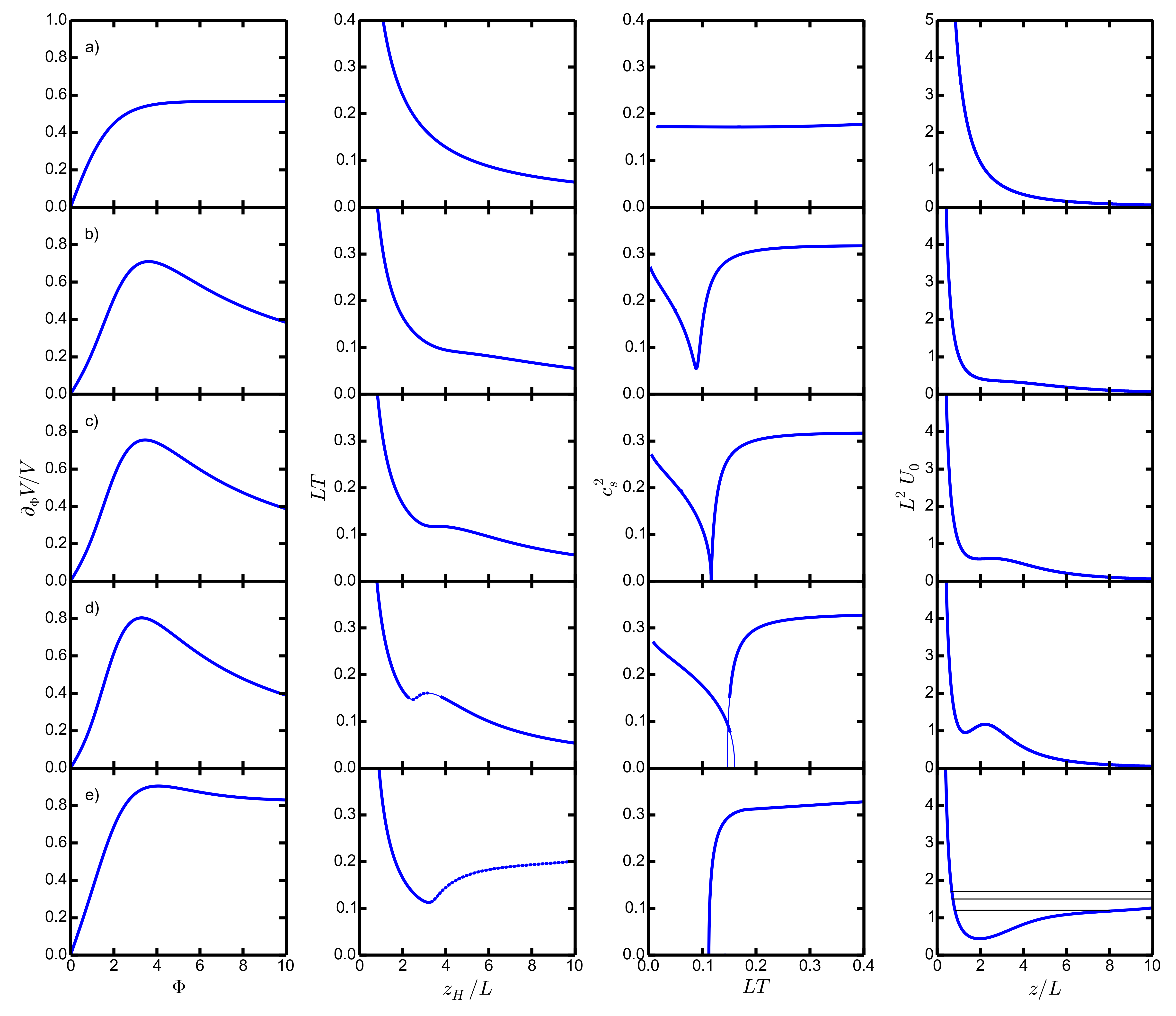
Figure 1: Selected examples of parameter choices (see Table 1) for the dilaton potential (15) (left column, for $\partial_{\Phi}V/V$), the resulting temperature $LT$ as a function of horizon position $z_{H}/L$ (second column), velocity of sound squared $c_{s}^{2}$ as a function of temperature $LT$ (third column) and the Schrödinger potential $L^{2}U_{0}$ as a function of $z/L$ (right column). The dilaton potential (15) serves as an input to solve the field equations (4-6) and obtain $T(z_{H})$ from (3), $c_{s}^{2}(T)$ from (8) combined with (3), and $U_{0}(z)$ from (14).

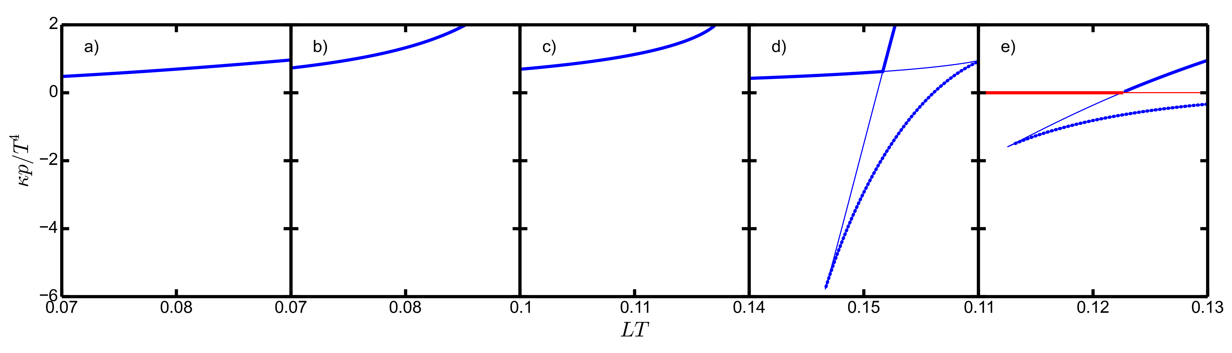
Figure 2: Scaled pressure $\kappa p/T^{4}$ as a function of $LT$ for the selected examples shown in Figure 1. The red lines in panel e) are for the thermal gas solution ($f=1$), where $p=0$ is employed (red lines). Meta (unstable) sections are depicted by thin (dotted) curves.

Example	$\gamma$	$a$	$b$	$\Delta$	Transition
a)	0.56	-0.077	0	2.63	none
b)	0	1.155	0.18	3.3	cross-over
c)	0	1.155	0.20	3.3	second-order
d)	0	1.155	0.25	3.3	first-order
e)	0.83	-2.69	0	3.06	Hawking-Page

Table 1: Parameter selection yielding the examples in Figure 1 and the characterization of the thermodynamic features.

As already remarked in mimi , quite featureless dilaton potentials $V(\Phi)$ can lead to fairly different thermodynamic features. Since the field equations (4-6) can be rearranged to display only a sensitivity to $\partial_{\Phi}V/V$ as a function of $\Phi$, we plot this key quantity in the left column of Figure 1. Example a) does not exhibit any features: $T(z_{H})$ is monotonously decreasing, $c_{s}^{2}(T)$ is increasing, and $U_{0}$ has no minimum, meaning that normalizable modes as probe vector mesons do not exist at all. Examples b) - d) exhibit $\partial_{\Phi}V/V$ with a pronounced maximum which becomes gradually higher. In case b), $T(z_{H})$ is monotonously dropping, albeit with a shallow near-flat section; it causes a pronounced minimum of the sound velocity squared; $U_{0}$ does not allow for any normalizable states due to the lacking minimum. That case is classified as cross-over. Case c) features a lifted maximum of $\partial_{\Phi}V/V$, resulting in a flat section of $T(z_{H})$, and the sound velocity drops at a certain temperature to zero, thus representing an example of a second-order phase transition. The Schrödinger equivalent potential $U_{0}(z)$ has here a very shallow minimum, i.e. probe vector mesons as normalizable modes cannot show up. Lifting the maximum of $\partial_{\Phi}V/V$ further (case d)), $T(z_{H})$ shows a local minimum that is connected to an inflection point, implying metastable states, unstable states and spinodales as well. That becomes most evident by the sound velocity squared $c_{s}^{2}(T)$ and the pressure $p(T)$ (see Figure 2): metastable states are depicted by thin solid curve sections and the unstable ones by dotted sections. Clearly, states with $c_{s}^{2}<0$ cannot be realized in nature. All these features classify a first-order phase transition, for which $U_{0}(z)$ exhibits a local minimum; it is - for the given parameters - still too shallow to accommodate vector mesons. Only if $\partial_{\Phi}V/V$ exceeds $\sqrt{2/3}$ (case e)), the global minimum of $U_{0}(z)$ allows for meson states, depicted by horizontal lines. At the same time, $T(z_{H})$ has a global minimum pointing to a Hawking-Page (HP) phase transition. Let be $T_{\min}=\min T$ at $z_{H}^{\min}$. Then, the branch for $z_{H}<z_{H}^{\min}$ is stable (for $p>0$) and metastable (for $p<0$), while the branch for $z_{H}>z_{H}^{\min}$ is unstable, and its free energy is above the thermal gas solution (see kir1 for the related construction) which applies for $0<T<T_{\min}<T_{\rm c}<\infty$, where $T_{\rm c}$ (slightly above $T_{\min}$) is the first-order phase transition temperature. (While $T_{\min}$ follows as minimizer of (3) over $z_{H}$, $T_{\rm c}$ is obtained by the loop construction sketched in the rightmost graphs of Figure 2.) The velocity of sound drops to zero at $T_{\rm c}$.
These examples are selected to have a survey on the thermodynamics and holographic quantities which can be uncovered by (15). This information is refined in Subsection IV.1, where we provide a systematic scan through the planes $\gamma=$constant and $b=$constant.
Figures 3 and 4 exhibit that region in the $\gamma$-$a$-$b$ parameter space, where a first-order or HP phase transition occurs; and in Figure 4, curves on which a second-order phase transition happens are depicted too. Thanks to the three-parameter potential (15), the visualization of the parameter space structure is quite straightforward, while multi-parameter ansätze may lead to intricate structures. In the present case, the HP transition happens for $\gamma\geq 0.8$ for all BF permitted values of $a$ and $b$ as well, as exhibited in the left panel of Figure 4. For $\gamma<0.8$, the blue areas depict the first-order phase transition, which are limited by the second-order transition (red curves). Further left (gray parts of the panels with constant $\gamma$ or $a$ or $b$ cross sections), a cross-over occurs, which turns smoothly into a featureless behavior for smaller values of $b$.

III.2 Shaping the dilaton potential

For $\gamma=0.568$, $a=-1.92$ and $b=-0.04$, the potential (15) reproduces the Lattice QCD data baza of $c_{s}^{2}(T)$ fairly well when adopting the scale setting parameter $L^{-1}=1990$ MeV. These data and our fit are restricted to the range 125 MeV$<T<$450 MeV. The dependence $LT$ vs. $z_{H}/L$ looks nearly the same as in Figure 1, case b), while the combination $\partial_{\Phi}V/V$ as a function of $\Phi$ exhibits a local maximum at $\Phi\approx 1.4$ and a local minimum at $\Phi\approx 5$ and stays below 0.6, i.e. these details are somewhat different from that displayed in Figure 1, case b), left panel. The successful description of the sound velocity squared can be taken as argument for considering the potential (15) useful for catching essential QCD features.
We refrain from further quantitative comparison with QCD thermodynamics and refer the interested reader to kir1 ; mimi ; debye ; yaresko ; yaresko-knaute , for example, where the thermodynamics of Yang-Mills and 2+1 flavor QCD with physical quark masses is considered. The essence is to employ multi-parameter ansätze of the dilaton potential with the aim to reproduce the Lattice QCD thermodynamics results as good as possible. Information of QCD is thus imported and mapped in a cumulative manner on $V(\Phi)$ within such a bottom-up approach without explicit reference to quarks and gluons and their masses, colors, flavors, couplings etc. Having successfully accomplished the shaping of $V(\Phi)$, one can proceed to derive further quantities, such as viscosities pufu ; rocha , diffusion constants rouge ; rouge2 etc. as predictions. By extending the model (1) by further fields, e.g. a Maxwell type $U(1)$ gauge field wolfe ; yaresko-knaute ; knaute , one may address non-zero chemical potential effects to access the phase diagram and issues of a critical point. Here, susceptibilities serve as crucial further information to be imported from QCD too.
However, our present goal here is to answer the question whether one can describe – within the modeling (1, 9) – at the same time the LHC relevant QCD thermodynamic features, i.e. a cross-over at about 155 MeV borsa ; baza , and a proper in-medium behavior of hadrons, i.e. probe vector mesons as representatives thereof. By a proper “in-medium behavior” we mean that at chemical freeze-out temperature of about 155 MeV alice , hadrons do exist with hardly medium-modified properties. Otherwise, the famous thermo-statistical interpretation of hadron multiplicities in ultra-relativistic heavy-ion collisions alice would be invalidated.

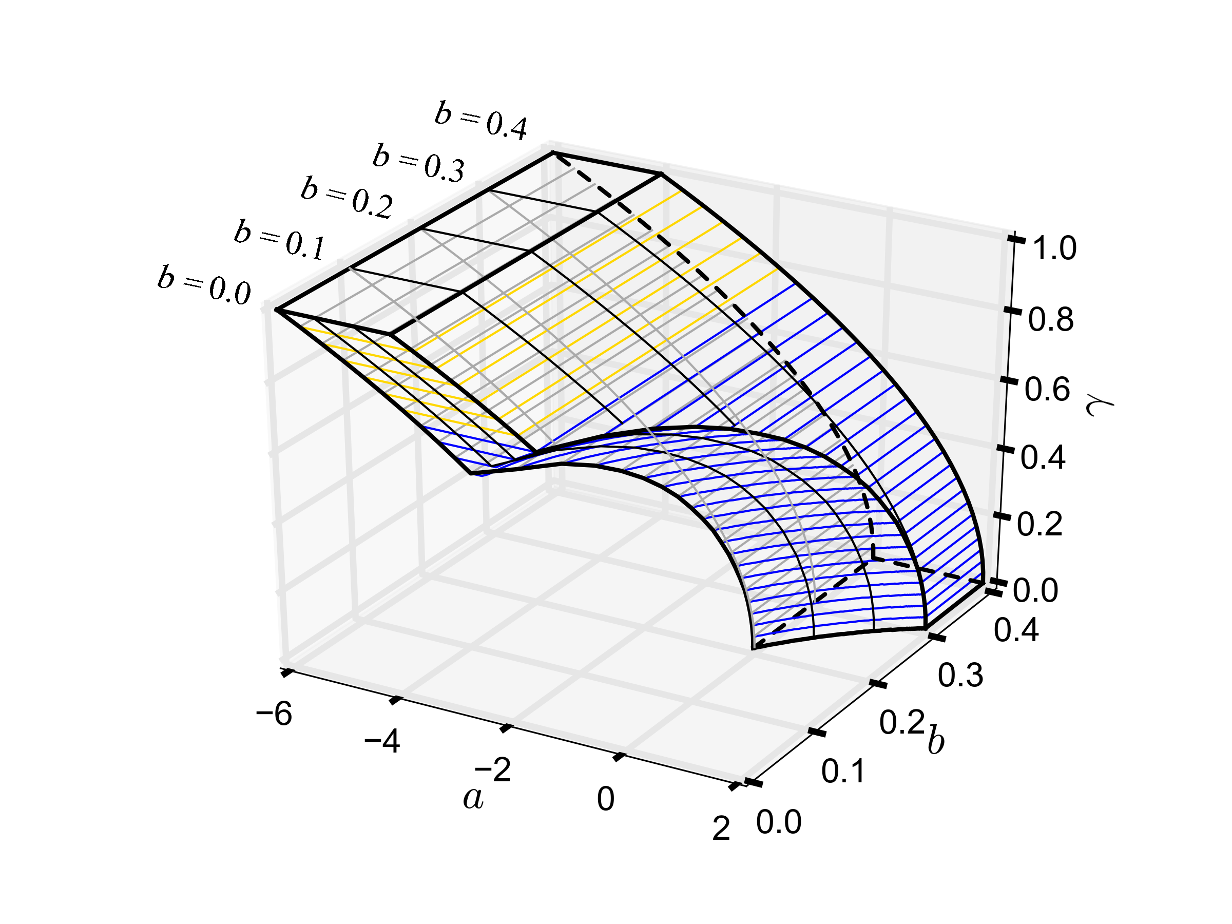
Figure 3: Plot of the region in the $\gamma$-$a$-$b$ parameter space, where a HP or first-order phase transition in the BF allowed range occurs for the dilaton potential (15). Cross sections of constant values of $\gamma$, $a$ and $b$ are exhibited in Figure 4.

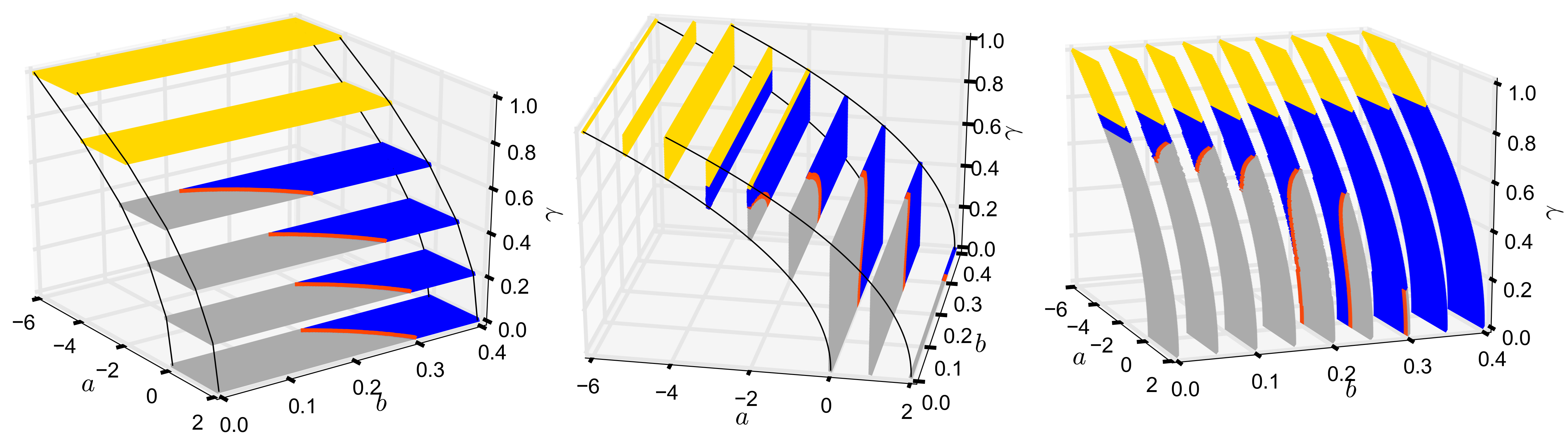
Figure 4: Plot of parameter ranges of the dilaton potential (15) for first-order phase transition (blue areas) or HP transition (yellow areas) for a series of selected constant values of $\gamma=0,\cdots$, 1 (left), $a=-6,\cdots,2$ (middle) and $b=0,\cdots,0.4$ (right). The red curves mark the second-order phase transition ranges; beyond, the transition turns into a cross-over, followed by a featureless behavior (dark gray areas). The BF bound restricts the values of $a$ to the strip $-6\gamma^{2}<a<2-6\gamma^{2}$ (depicted by the two black solid curves in left and middle panels). The panels continue to larger values of $b$ and $\gamma$ without changes.

The answer to the posed problem seems to be negative. Hints come, for example, from col12 ; col09 ; gherghetta ; kapusta ; bk , where the melting (disappearance) of hadrons was found to happen at temperatures significantly below 155 MeV. While ich2017 offers an avenue to remedy such an insanity, the given framework of (1, 9) seems to be too restricted and calls for extensions. Leaving the latter ones for separate work, we try to find a loophole to join the cross-over thermodynamics and suitable probe vector meson states. Prior to that, however, we attempt to clarify the systematics of thermodynamic features in the spirit of the last column of Tab. 1 in relation to the dilaton potential.

III.3 Beyond the adiabatic approximation

The authors of mimi derived the relation (henceforth called Gubser’s adiabatic criterion)

$$c_{s}^{2}\approx\frac{1}{3}-\frac{1}{2}\left(\frac{\partial_{\Phi}V}{V}\right)^{2},$$ (16)

where ‘$\approx$‘ indicates the validity in adiabatic approximation. The formula implies that for $\partial_{\Phi}V/V>\sqrt{2/3}$ the sound velocity becomes imaginary, thus pointing to a first-order phase transition, either as a standard construction $\rm\grave{a}$ la example d) or the HP transition $\rm\grave{a}$ la example e) in Figure 2. To systematize the various thermodynamic scenarios, we plot $\partial_{\Phi}V/V$ of the above examples a) - e) in one diagram, see Figure 5. Based on such a comparison, the impact of $\partial_{\Phi}V/V$ on the thermodynamics can be summarized qualitatively as follows: If $\partial_{\Phi}V/V$ reaches the value $\sqrt{2/3}$ (or somewhat below, depending on the concrete $V(\Phi)$), $T(z_{H})$ forms a local extremum, where the nearest one to the boundary becomes a minimum. So if $\partial_{\Phi}V/V$ intersects the $\sqrt{2/3}$ line once, we have a global minimum of $T(z_{H})$ and a HP phase transition. Otherwise, if $\partial_{\Phi}V/V$ intersects twice, $T(z_{H})$ forms a local minimum followed by a local maximum and we have a first-order phase transition. A second-order phase transition arises if $\partial_{\Phi}V/V$ touches the $\sqrt{2/3}$ line. Additionally, each extreme point of $\partial_{\Phi}V/V$ implies an inflection point of $T(z_{H})$, i.e. a cross-over is generated by a maximum of $\partial_{\Phi}V/V$ whose altitude stays below $\sqrt{2/3}$.
To formalize these findings we derive in Appendix A the relation

$$\frac{1}{T}\frac{\mathrm{d}T}{\mathrm{d}z_{H}} = \frac{1}{2}\frac{V}{\partial_{\Phi}V}\left(\left(\frac{\partial_{\Phi}V}{V}\right)^{2}-\frac{2}{3}\right)\Phi^{\prime}$$ (17)

$$+\frac{\partial A}{\partial z_{H}}+\left(\frac{3}{2}\frac{\partial A^{\prime}}{\partial z_{H}}+\Phi^{\prime}\frac{\partial\Phi}{\partial z_{H}}\right)\frac{\partial_{\Phi}V}{V},$$

where $\Phi^{\prime}\equiv(\partial_{z}\Phi(z,z_{H}))\mid_{z=z_{H}}$, $A^{\prime}\equiv(\partial_{z}A(z,z_{H}))\mid_{z=z_{H}}$.

Figure 5: Left: Comparison of the dilaton potentials of examples a) - e) in Figure 1 for $\Phi=0\cdots 5$. The horizontal line is the adiabatic criterion (16). Right: Comparison of Gubser’s criterion and the $T_{\min}$ curve which shows the minimum value of $\partial_{\Phi}V/V$ as a function of $\Phi_{H}$ for which $T(z_{H})$ displays a minimum pointing to a first-order or HP transition. If $\partial_{\Phi}V/V$ as a function of $\Phi$ exceeds the $T_{\min}$ curve, then $T(\Phi_{H})$ exhibits a minimum; otherwise, if $\partial_{\Phi}V/V$ stays below the $T_{\min}$ curve, $T(\Phi_{H})$ decreases monotonously which points to a cross-over transition or to featureless thermodynamics. (In detail, for the dilaton potential (15) with $\gamma=b=0$ and a given value of $a$ with $0\leq a\leq 2$, $T(\Phi_{H})$ is computed as well as the position of its minimum $\Phi_{H}^{\min}(a)$. The $T_{\min}$ curve then is the connection of all points $\left(\Phi_{H}^{\min},\partial_{\Phi}V/V(\Phi_{H}^{\min})\right)$ for running values of $a$.)

Given the facts that (i) $T(z_{H}\to 0)\to\frac{1}{\pi z_{H}}$ cherman ; hohler , (ii) the monotonous behavior of $\Phi(z,z_{H})$ as a function of $z$ with $\Phi^{\prime}>0$, and (iii) the above quoted asymptotic behavior of $V(\Phi)$ at small $\Phi$ (implying $\partial_{\Phi}V/V=m_{\Phi}^{2}L^{2}\Phi/12$), one recognizes from the first line of (17) that the slope $\mathrm{d}T/\mathrm{d}z_{H}$, which is negative at small $z_{H}$, can turn into a positive one, once $\partial_{\Phi}V/V>\sqrt{2/3}$ is reached, indicating a local or global minimum of $T(z_{H})$. Understanding “adiabatic approximation” as a situation where $\partial A/\partial z_{H}$, $\partial A^{\prime}/\partial z_{H}$ and $\partial\Phi/\partial z_{H}$ are small, one thus recovers Gubser’s adiabatic criterion. Otherwise, the second line of (17) provides corrections. In fact, in example d), $\partial_{\Phi}V/V$ stays below the $\sqrt{2/3}$ line but facilitates a first-order phase transition. (The relation of $T(z_{H})$ to transitions is discussed in exp1 ; exp2 : in essence, a minimum of $T(z_{H})$ points to a first-order phase transition, since $s(z_{H})$ is a monotonously increasing function.) The corrections give eventually a border line (called $T_{\min}$ curve) for each type of dilaton potential which is determined by calculating the minimum value of $\partial_{\Phi}V/V$ (as a function of $\Phi$ and depending on all parameters denoted shortly by $\vec{p}\,$) such that $T(z_{H})$ forms a minimum. Systematic numerical analyses with the dilaton potential (15) show that this line is shifted down if $\partial_{\Phi}V/V$ as a function of $\Phi$ becomes steeper when varying the parameters $\vec{p}$ in $V(\Phi;\vec{p})$. The right part of Figure 5 shows an example of such a line and the dependence of the difference between Gubser’s criterion and the $T_{\min}$ curve as a function of $\Phi$. This is further visualized in Figure 6 for two special parameters, $b=0$ and 2, in the projections on the $\gamma$-$a$ plane: the offset of the regions determined by (16) and the true onset of a first-order phase transition increases with $b$; in addition, the region where the Schrödinger equivalent potential $U_{0}$ displays a minimum is shown by the red curves.

Figure 6: Projection of border lines (for $b=0$ and $b=0.2$) of parameter regions on $\gamma$ vs. $a$ plane, where $T(z_{H})$ has a minimum (blue hatched regions, left and above to solid blue curves), $U_{0}$ has a minimum (left and above to red curves), and $\partial_{\Phi}V/V$ is greater than $\sqrt{2/3}$ (left and above to dashed blue curves) for the dilaton potential (15); if $b$ and therefore the slope of $\partial_{\Phi}V/V$ increase, the difference between Gubser’s adiabatic criterion (blue dashed) and the $T_{\min}$ curve (solid blue) becomes larger. In the blue double-hatched region, $\gamma$ is great enough to have a first-order phase transition for all $a$ and $b$. The region of a HP transition is in yellow. The green hatched regions are excluded due to BF.

IV Schrödinger potential

IV.1 Adiabatic approximation to Schrödinger equivalent potential

The relationship between the situation of $T=0$ and features at $T>0$ has been stressed in exp1 ; exp2 . Here, we envisage a relation of $U_{0}(z)$ and $T(z_{H})$ in adiabatic approximation. In Appendix B we derive the relation

$$9U_{0}\cong\frac{17}{12}\frac{T^{\prime 2}}{T^{2}}+\frac{28}{3}\pi T^{\prime}+\frac{44}{3}\pi^{2}T^{2}+2\left(2\pi T-\frac{T^{\prime}}{T}\right)\sqrt{\frac{8}{3}\left(\frac{T^{\prime 2}}{T^{2}}+5\pi T^{\prime}+4\pi^{2}T^{2}\right)}.$$ (18)

It is valid if, in a decomposition $A(z,z_{H})=A_{0}(z)+a(z,z_{H})$ and $\Phi(z,z_{H})=\Phi_{0}(z)+\varphi(z,z_{H})$, where $A_{0}$ and $\Phi_{0}$ denote the solutions of (4)-(6) in case of $f=1$ and the terms $a(z,z_{H})$ and $\varphi(z,z_{H})$ are sub-leading and can be neglected. The Chamblin-Reall solution CR with $V(\Phi)\propto\exp\{\gamma\Phi\}$ is an example, where $a=\varphi=0$ can be chosen, despite of $f(z,z_{H})\leq 1$.
Equation (18) is exact for the AdS-BH metric, i.e. $A=-2\ln(z/L)$, $\Phi(z)=0$ and $f(z,z_{H})=1-(z/z_{H})^{4}$ which is generated by $V(\Phi)=-12/L^{2}$. Moreover, the left side converges against the right side, if (i) $z\to 0$ because $A(z\to 0,z_{H})\to-2\ln(z/L)$ and $\Phi(z\to 0,z_{H})\to 0$ for all $z_{H}$ and (ii) $z\to\infty$ due to $A\to A_{0}$, $\Phi\to\Phi_{0}$ and the implied large values of $z_{H}$.
If we assume that $T(z_{H})$ has a minimum at $z_{H}=z_{H}^{\min}$, (18) yields $U_{0}^{\prime}(z=z_{H}^{\min})=\frac{\pi}{3}(43-8\sqrt{6})T^{\prime\prime}>0$ meaning $U_{0}$ increases at the minimum position of $T$. Due to the AdS asymptotics of the Schrödinger potential, $U_{0}^{\prime}(z\to 0)\propto-z^{-3}<0$, there has to be a minimum of $U_{0}(z)$ as well, at a position nearer to the boundary, i.e. in the interval $0<z<z_{H}^{\min}$. While derived within the above approximations, and thus not as rigorous as a no-go-theorem, one could argue that a minimum of $T(z_{H})$ (which is related to a HP or first/second-order transition) is consistent with a minimum of $U_{0}(z)$. The reversed clue (though not necessarily true in any case, cf. Figure 1c) is demonstrated by an example in the next subsection.
Before requiring a minimum of $U_{0}(z)$, let us consider the reason for the disappearance of the $U_{0}$ minimum for certain parameter settings. The UV region of $U_{0}(z)$ is supposed to be determined by the near boundary behavior of $A_{0}(z)$, while the IR behavior is supposed to be determined essentially by the dilaton field. If true, then a piecewise shape $\Phi_{0}(z)\propto z^{p+1}$ generates a contribution $\propto z^{2p}$ to leading order $U_{0}$ in the IR. If such a term is dominating, then $U_{0}\propto z^{2p}$, i.e. $p>0$ is needed arrive at a shape of $U_{0}$ in the IR with $\partial U_{0}/\partial z>0$. To quantify such a rough consideration (which ignores the coupling of $\Phi$ and $A$ via (5)) we have scanned through the parameter space of (15) on two representative directions, see Figure 7. In doing so, we see in fact that only in the region of a first-order or second-order or Hawking-Page phase transition (cf. Figure 4) the rise of the dilaton field in $z$ direction is strong enough to enforce also the IR rise of $U_{0}$, meaning that only in such cases $U_{0}$ can exhibit a pronounced minimum which is the prerequisite to allow for normalizable solutions of (10) at $T=0$. Figure 7 offers a better understanding of the deformations of the various quantities, e.g. $c_{s}^{2}(T)$ or $T(\Phi(z_{H}))$ or $U_{0}(z)$, under continuous changes of the dilaton potential parameters, thus supplementing Figure 1.

Figure 7: A scan through the planes $\gamma=0.5$, $a=0$ (left column, compare Figure 4-left) and $b=0.2$, $\Delta=2$ (right column, compare Figure 4-right) by selecting a few values of the remaining parameters of (15) to exhibit the induced change of $\partial_{\Phi}V/V$ as function of $\Phi$, $LT$ as a function of $\Phi(z_{H})$, $c_{s}^{2}$ as a function of $LT$, $\Phi$ as a function of $z/L$ and $L^{2}U_{0}$ as a function of $z/L$ (from top to bottom). The line style is as in Figure 1; values of the remaining parameters:

line color	blue	green	red	cyan
$b$ (left column)	0.3	0.18	0.1	0
$a$ (right column)	0.83	0.65	0.5	0.3

IV.2 Requiring a minimum of $\boldsymbol{U_{0}(z)}$

The above examples demonstrate that for many parameter choices of the dilaton potential $V(\Phi)$ the Schrödinger potential $U_{0}(z)$ does not exhibit a minimum and thus does not allow for modes which can be interpreted as probe vector mesons. Instead of deriving the background (warp factor and dilaton profile at $T=0$) from given dilaton potential, we start now with an ansatz for $U_{0}(z)$ such as to have a minimum. Assuming the latter one is sufficiently deep, normalizable modes would then be expected. Our ansatz for demonstrative purposes is

$$U_{0}(z)=\frac{3}{4z^{2}}+\left(\frac{z}{L}\right)^{p}\frac{1}{L^{2}},$$ (19)

where the first term comes from the asymptotic warp factor at $z\to 0$; the second term facilitates the required minimum at $z_{\min}/L=(3/2p)^{\frac{1}{p+2}}$ with $L^{2}U_{0}^{\min}=(3/2p)^{\frac{p}{p+2}}(1+p/2)$. Equation (12) is solved at $f=1$ by

$$\mathcal{S}_{0}=2\frac{\mathrm{d}}{\mathrm{d}\hat{z}}\ln\left(c_{1}\hat{z}^{-\frac{1}{2}}\,_{0}F_{1}\left(\frac{p}{p+2},\frac{\hat{z}^{p+2}}{(p+2)^{2}}\right)+c_{2}\hat{z}^{\frac{3}{2}}\,_{0}F_{1}\left(\frac{p+4}{p+2},\frac{\hat{z}^{p+2}}{(p+2)^{2}}\right)\right)$$ (20)

with $\hat{z}\equiv z/L$ and $c_{1}=1$ (due to AdS behavior at boundary $z\to 0$) and $c_{2}=-\frac{1}{2}(p+2)^{\frac{p-2}{p+2}}\Gamma(\frac{p}{2+p})/\Gamma(\frac{2}{p+2})$ (due to the assumption that (19) is globally valid). The field equations (4-6) must be solved numerically to get $A(z)$, $\Phi(z)$ and $V(\Phi)$. The same $V(\Phi)$, which is supposed to be independent of $T$, is then used to derive $U_{T}(z,z_{H})$ and $T(z_{H})$. Figure 8 exhibits such solutions for $p=0.5$, 1 and 2, where the latter value reproduces the soft-wall model KKSS with a strictly linear Regge type spectrum $L^{2}m_{n}^{2}=4(n+1)$ for $n=0,1,2\cdots$. The left panel is for $U_{0}(z)$ according to (19), while the middle panel shows $T(z_{H})$; the right panel displays $\partial_{\Phi}V/V$ as a function of $\Phi$. There is a striking similarity of the curves $T(z_{H})$ and $U_{0}(z)$ (isotopy referring to the monotony behavior) which we interpret as follows: a minimum of $U_{0}(z)$ is related to a minimum of $T(z_{H})$, i.e. a first-order phase transition - here a HP transition, since it is a global minimum. The behavior of $\partial_{\Phi}V/V$ as a function of $\Phi$ is in agreement with our assessments in Sections III.1 and III.3.

Figure 8: $L^{2}U_{0}$ as a function of $z/L$ (left panel), $LT$ as a function of $z_{H}/L$ (middle panel), and $\partial_{\Phi}V/V$ as a function of $\Phi$ (right panel) for the input (19). Red solid/green dashed/black dotted curves are for $p=2$/1/0.5.

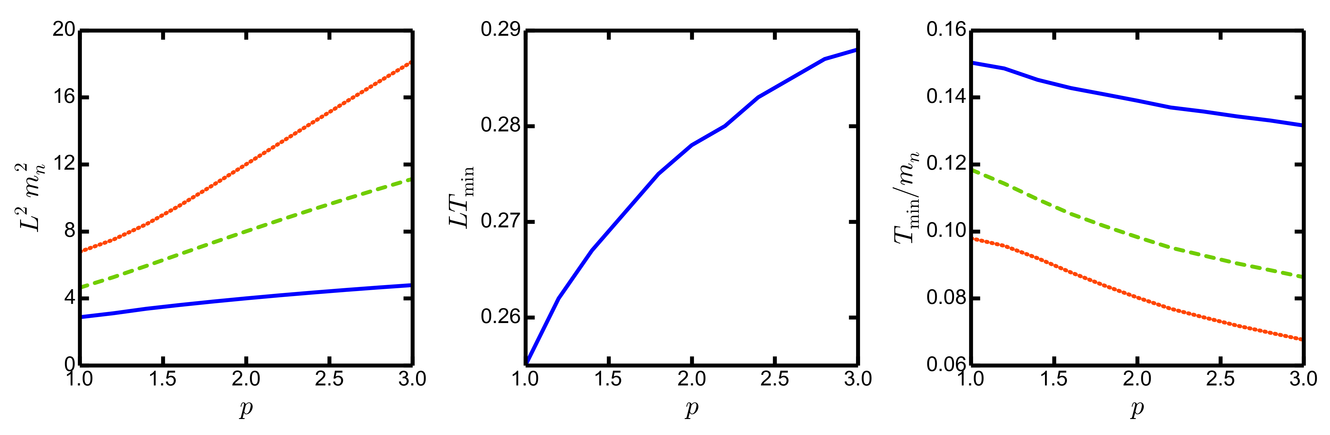
Figure 9: Scaled vector meson masses squared $L^{2}m_{n}^{2}$ as a function of $p$ (left panel), scaled minimum temperature $LT_{\min}$ as a function of $p$ (middle panel), and ratio $T_{\min}/m_{n}$ as a function of $p$ for the ansatz (19). Blue solid/green dashed/red dotted for ground state/first excitation/second radial excitation (there is an infinite tower of excitations for all $p$).

To get an idea on the related scale, the left-hand plot of Figure 9 shows the first three states, that is $L^{2}m_{n}^{2}$ as a function of $p$ for $n=0$ (ground state) and $n=1$, 2 (first two radial excitations). For comparison, the middle plot of Figure 9 displays $LT_{\min}$ also as a function of $p$. Both figures can be combined to $T_{\min}/m_{n}$ as a function of $p$ (right-hand plot of Figure 9). Having in mind applications to QCD and identifying $T_{\min}$ with 155 MeV (see above) and $m_{0}$ with the $\rho$ meson ground state mass of 770 MeV, one arrives at $T_{\min}/m_{0}\approx 0.20$, i.e. a value not too far from the range of values shown in the right-hand plot of Figure 9. However, 2+1 flavor QCD with physical quark masses does not provide a first-order phase transition. Insofar, the present set-up is more appropriate for 2+1 flavor QCD in the chiral limit, which in fact enjoys a first-order phase transition philipsen2018 ; ding , but detailed information on thermodynamic quantities as well as the vector meson spectrum is lacking (cf. Karsch for a search for the delineation curve in the Columbia plot where cross-over and first-order phase transitions touch each other; very preliminary first estimates schmidt point to a ratio of $T_{\rm c}/m_{0}$ in the same order of magnitude as for the case of physical quark masses); $T_{\rm c}$ becomes in the chiral limit $\approx 132$ MeV ding .
The temperature dependence of $U_{T}$ (not shown) is such to cause the instantaneous disappearance (melting) of vector meson states at $T_{\rm c}\approx T_{\min}$ (see Figure 10). Denoting the disappearance temperature by $T_{\rm dis}$ and choosing $m_{0}=m_{\rho}$ as scale, Figure 10 translates into $T_{\rm dis}=m_{\rho}\frac{LT_{\rm dis}}{Lm_{0}}$, meaning $T_{\rm dis}=116$ MeV for $LT_{\rm dis}=0.27\,(0.3)$ and $Tm_{0}=1.7\,(2)$. That value of $T_{\rm dis}$ does not apply to 2+1 flavor QCD with physical quark masses, since, as stressed above, the present scenario is more suitable for the chiral limit where a first-order phase transition occurs.

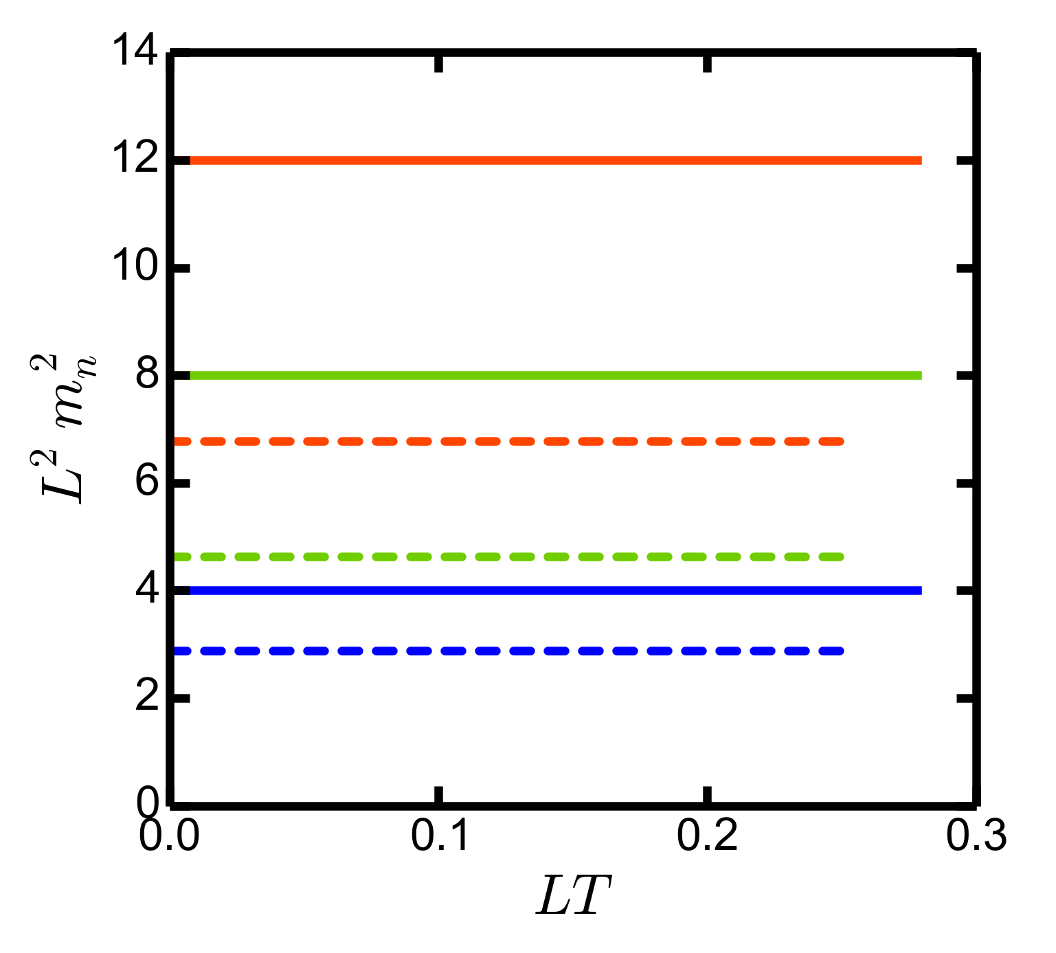
Figure 10: Vector meson masses squared $L^{2}m_{n}^{2}$ of the first three states (color code as in Figure 9) as a function of the temperature for the parameter $p=2$ (solid) and $p=1$ (dashed). The masses are constant during the thermal gas phase and all excitations disappear at $T_{\rm c}$, where the black hole solution begins to apply.

V Summary and discussion

We focus here on the QCD relevant cross-over transition and its discrimination against first-order and second-order transitions. Obviously, more complicated structures are possible, e.g. a sequence or nested first-order transitions for functions $T(z_{H})$ with multiple local minima (see kir1 for the case of a double transition). These require further shaping of the dilaton potential. This can be easily done by combining the elements of our systematics presented in this paper: an extreme point of $\partial_{\Phi}V/V$ generates an inflection point of $T(z_{H})$ which points to a cross-over or a second-order phase transition (if it is a horizontal turning point) or to a first-order phase transition if the temperature exhibits additional extreme points which can be controlled by the altitude of $\partial_{\Phi}V/V$.
We did not touch such issues as good and bad curvature singularities singular , adding further (e.g. charged scalar) fields which can bridge to order parameters and/or condensation cubro , larger classes of dilaton potentials (e.g. Liouville potentials or linear combination thereof kirfr ) and fluctuations.
Unfortunately, the Einstein gravity - dilaton model seems to be not flexible enough to allow simultaneously for a cross-over and probe meson states because the existence of the latter ones requires a minimum in $T(z_{H})$. The obvious idea to construct a dilaton potential such that $T(z_{H})$ has a minimum at a horizon $z_{H}^{*}$ with $T(z_{H}^{*})$ being small (to ensure the existence of the mesons) and a cross-over at the QCD critical temperature of about 155 MeV does not work very well, since all probe mesons states disappear already at the minimum temperature $T(z_{H}^{*})$. However, keeping the background, as determined in Section III, a refinement of the action (9) has the capability of describing properly (i) probe vector mesons at low temperatures and (ii) the pattern of meson melting at high temperatures, consistent with lattice QCD. The details will be reported elsewhere.
A first step further on the road to a fully consistent approach could be the consideration of a $U(1)$ Maxwell type gauge field. Such a field has been used to address the question of the behavior of probe vector mesons in relation to the thermodynamics: $\rho$ mesons are described through the $U(1)$ gauge field (see (9)) and putting together the actions (1) and (9) would yield a model with full back reaction from the mesons to the gravity background.
Since QCD thermodynamics is not driven by vector mesons alone, another step is adding systematically flavor, e.g. by including the pseudo-scalar and scalar sectors via the bulk fundamental fields and its vacuum expectation values. Some works point directly in this direction: the authors of bk2 introduce a second scalar field (glue ball field) and solve the field equations for the case $T=0$; many other investigate the behavior of hadron species in a given background without back reaction (see e.g. col12 ; col09 ; cui11 ; cui13 ; lee09 ; fuj09 ; mir09 ; ich2016 ; csaki ). yamaguchi ; fang give a study of phase transitions in relation to a flavor containing model with given metric background. Back reactions are accounted for in the V-QCD model class pioneered in vqcd , where the flavor sector supplements the gluon (dilaton) sector, thus catching many desired features in relation to QCD, up to the equation of state adapted to the 2+1 flavor case for $T>T_{\rm c}$ (cf. vqcd2 and further references therein). Bringing the characteristic features of the mentioned works together would be an improvement. The Holy Grail would be a model with parameters steering quark masses and condensates for different flavors separately with proper hadron spectra in all (scalar, pseudo-scalar, vector, axial-vector, tensor and axial-tensor) sectors.
All mentioned extensions point to the leading question, which framework is needed to have a QCD consistent thermodynamics and proper in-medium modifications of the hadron species. However, increasing the variety of a model means increasing its complexity and requires much follow-up work.

Appendix A Derivation of (17)

We use $f^{\prime}(z_{H},z_{H})=-4\pi T(z_{H})$ and $f(z_{H},z_{H})=0$ to evaluate (6) and (7) at $z=z_{H}$ which imply

$$T(z_{H}) = \frac{1}{6\pi}\frac{e^{A(z_{H},z_{H})}}{A^{\prime}(z_{H},z_{H})}V(\Phi(z_{H},z_{H})),$$ (21)

$$T(z_{H}) = -\frac{1}{4\pi}\frac{e^{A(z_{H},z_{H})}}{\Phi^{\prime}(z_{H},z_{H})}\partial_{\Phi}V(\Phi(z_{H},z_{H})),$$ (22)

respectively. Differentiating (21) w.r.t. $z_{H}$ yields

$$\frac{1}{T}\frac{\mathrm{d}T}{\mathrm{d}z_{H}}=A^{\prime}+\frac{\partial A}{\partial z_{H}}-\frac{1}{A^{\prime}}\left(A^{\prime\prime}+\frac{\partial A^{\prime}}{\partial z_{H}}\right)+\frac{\partial_{\Phi}V}{V}\frac{\mathrm{d}\Phi}{\mathrm{d}z_{H}},$$ (23)

where all functions are to be taken at $(z_{H},z_{H})$. Equating (21) and (22) yields $A^{\prime}$ at $z=z_{H}$ as

$$A^{\prime}\mid_{z=z_{H}}=-\frac{2}{3}\Phi^{\prime}\frac{V}{\partial_{\Phi}V}\mid_{z=z_{H}}.$$ (24)

By inserting (24) in (23) and eliminating $A^{\prime\prime}$ via (5) we find

$$\frac{1}{\Phi^{\prime}T}\frac{\mathrm{d}T}{\mathrm{d}z_{H}}=\frac{1}{2}\frac{\partial_{\Phi}V}{V}-\frac{1}{3}\frac{V}{\partial_{\Phi}V}+\frac{1}{\Phi^{\prime}}\frac{\partial A}{\partial z_{H}}+\frac{1}{\Phi^{\prime}}\left(\frac{3}{2\Phi^{\prime}}\frac{\partial A^{\prime}}{\partial z_{H}}+\frac{\partial\Phi}{\partial z_{H}}\right)\frac{\partial_{\Phi}V}{V}$$ (25)

at $z=z_{H}$. This leads directly to (17). The next step is to solve the field equation (4):

$$f(z,z_{H})=1-\frac{h(z,z_{H})}{h(z_{H},z_{H})},$$ (26)

where $h(z,z_{H}):=\int\nolimits_{0}^{z}\exp(-3/2A(\tilde{z},z_{H}))\,\mathrm{d}\tilde{z}$. This solution is well defined and can be employed to compute the temperature a for third time:

$$T(z_{H})=\frac{1}{4\pi}\frac{e^{-\frac{3}{2}A(z_{H},z_{H})}}{h(z_{H},z_{H})}.$$ (27)

After differentiating (21) w.r.t. $z_{H}$ and some manipulations we end at

$$\frac{1}{T}\frac{\mathrm{d}T}{\mathrm{d}z_{H}}+4\pi T=-\frac{3}{2}(A^{\prime}+\frac{\partial A}{\partial z_{H}})\mid_{z=z_{H}}+\frac{3}{2h}\int\limits_{0}^{z_{H}}\frac{\partial A}{\partial z_{H}}(\tilde{z},z_{H})e^{-\frac{3}{2}A(\tilde{z},z_{H})}\,\mathrm{d}\tilde{z}$$ (28)

which we will use in Appendix B.

Appendix B Derivation of (18)

We start with (14). To relate $U_{0}$ with $T$, we evaluate (21, 22, 25, 28) in leading order, i.e. neglecting $a$ and $\varphi$:

$$T = \frac{1}{6\pi}\frac{e^{A_{0}}}{A_{0}^{\prime}}V(\Phi_{0}),$$ (29)

$$T = -\frac{1}{4\pi}\frac{e^{A_{0}}}{\Phi_{0}^{\prime}}\partial_{\Phi}V(\Phi_{0}),$$ (30)

$$\frac{1}{\Phi_{0}^{\prime}T}\frac{\mathrm{d}T}{\mathrm{d}z_{H}} = \frac{1}{2}\frac{\partial_{\Phi}V}{V}-\frac{1}{3}\frac{V}{\partial_{\Phi}V},$$ (31)

$$\frac{1}{T}\frac{\mathrm{d}T}{\mathrm{d}z_{H}}+4\pi T = -\frac{3}{2}A_{0}^{\prime}.$$ (32)

These four equations allow for eliminating all $A$’s and $\Phi$’s in (14). Finally we arrive at (18).

Appendix C Towards a systematic dilaton potential expansion analysis

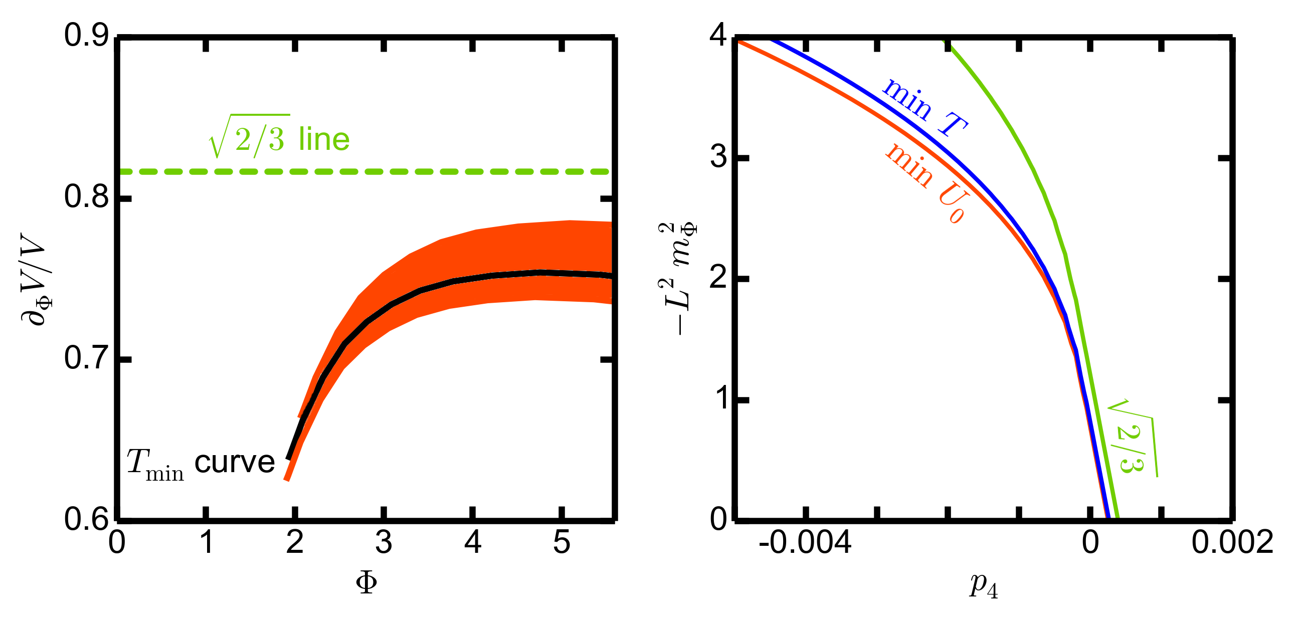
Figure 11: Left: $T_{\min}$ curve (solid black) generated by the potential (33) under variation of $p_{2}$ at $p_{i\geq 3}=0$, analogue to Figure 5. By varying a second parameter (here $p_{3}=-0.01\cdots 0.01$ and $p_{i\geq 4}=0$), the $T_{\min}$ curve becomes a strip (red area), where a negative (positive) value of $p_{3}$ belongs to the lower (upper) part, since increasing $p_{3}$ means increasing the slope of $\partial_{\Phi}V/V$ and therefore increasing also the difference between Gubser’s adiabatic criterion and the $T_{\min}$ curve. If $\partial_{\Phi}V/V$ as a function of $\Phi$ with given parameter set $\vec{p}$ has a section within the corresponding $T_{\min}$ area (here only displayed for a $p_{3}$ interval) then a first-order or HP phase transition is facilitated. Right: Border lines of parameter regions in $-L^{2}m_{\Phi}^{2}=p_{2}/24$ vs. $p_{4}$ space, where either $T(z_{H})$ has a minimum (right to blue curve), or $U_{0}(z)$ has a minimum (right to red curve), or $\partial_{\Phi}V/V$ is greater than $\sqrt{2/3}$ (right to green curve) for the dilaton potential (33) with $p_{3}=0$ and $p_{i\geq 5}=0$; if $m_{\Phi}$ and therefore the slope of $\partial_{\Phi}V/V$ increase, the difference between Gubser’s adiabatic criterion and the $T_{\min}$ curve becomes larger.

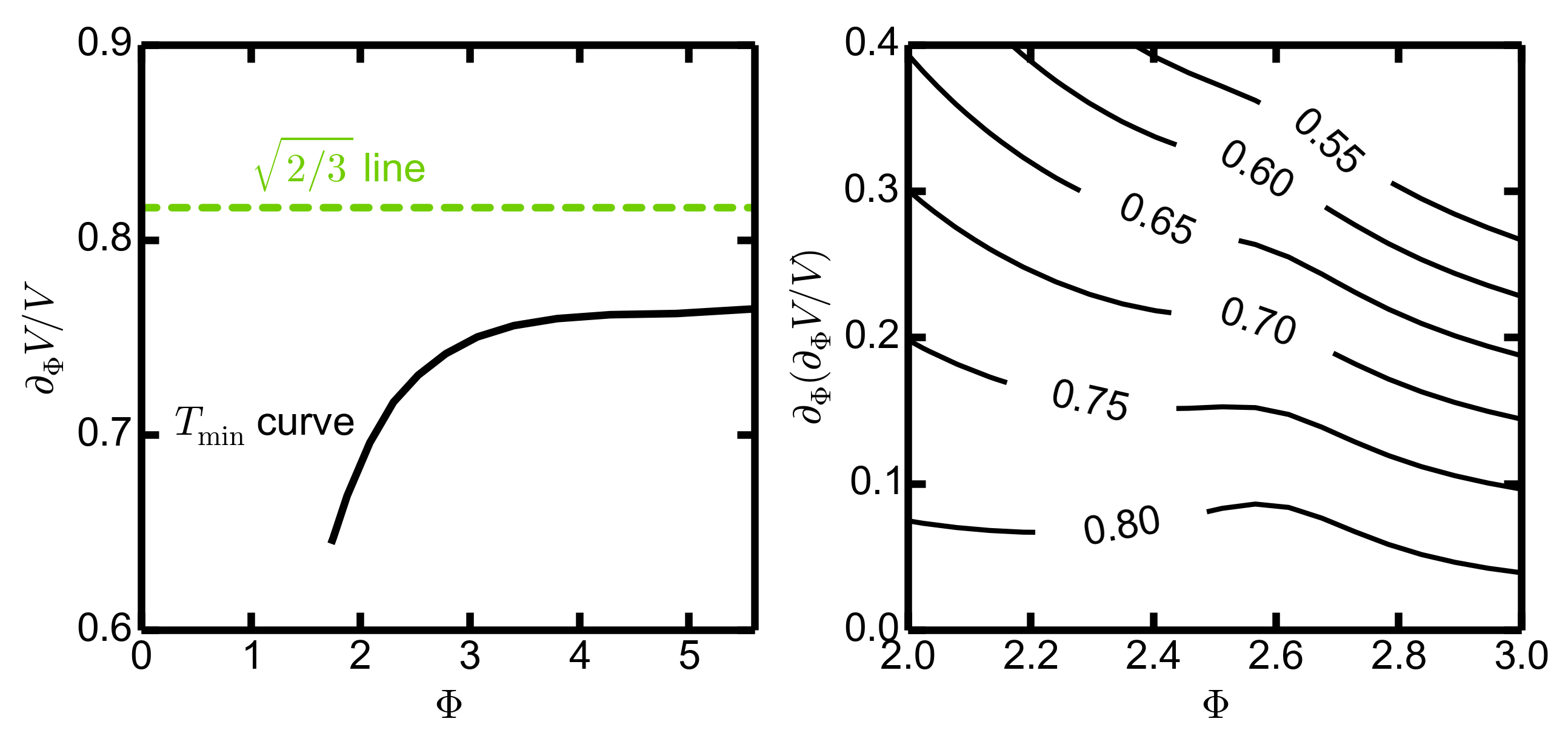
Figure 12: Left: $T_{\min}$ curve (solid black) generated by the potential (34) under variation of $\phi_{2}$ at $\phi_{4}=0.23$ and $\phi_{i\geq 6}=0$, analogue to Figure 5. Right: contour plot of the minimum value $(\partial_{\Phi}V/V)^{*}$ over the plane $\Phi$ vs. $\partial_{\Phi}(\partial_{\Phi}V/V)$ for which $T(\Phi_{H})$ exhibits a minimum: If $(\partial_{\Phi}V/V)$ exceeds this value (depending on its slope and the position) the temperature exhibits a minimum which is independent of the concrete set of parameters.

Another useful form of the dilaton potential is

$$-L^{2}V(\Phi)=12\exp\left(\sum\nolimits_{i=2}p_{i}\Phi^{i}\right),$$ (33)

since $\partial_{\Phi}V/V$ runs over all BF permitted and AdS conform polynomials if $\vec{p}=(p_{2},p_{3},\cdots)$ runs over all vectors. The case $p_{i\geq 3}=0$ characterizes the leading order (straight lines) in the spirit of an expansion of $\partial_{\Phi}V/V$ in powers of $\Phi$. The left panel in Figure 11 shows the influence of the varying $p_{3}$-depending term (red strip) on the $T_{\min}$ curve (black curve) which is generated with running $p_{2}$ analogously to Figure 5. The parameter regions in the $-L^{2}m_{\Phi}^{2}$ vs. $p_{4}$ plane, where $T(z_{H})$ (blue curve) or $U_{0}(z)$ (red curve) exhibits a minimum, as well as the area, where $\partial_{\Phi}V/V$ is greater than $\sqrt{2/3}$ (green curve), are also shown (see right panel and compare with Figure 6). In such a manner one can study, piece by piece, the impact of the individual terms in (33) on the issue of phase structure and capabilities to permit vector meson modes in the probe limit.
We complement the ansatz (33) by a purely polynomial form of $V(\Phi)$ in the spirit of a small-$\Phi$ expansion:

$$-L^{2}V(\Phi)=12+\sum\limits_{i=1}\phi_{2i}\Phi^{2i}$$ (34)

and vary the parameters $\phi_{2},\,\phi_{4}$ and $\phi_{6}$. A $T_{\min}$ curve is exhibited in Figure 12-left panel (cf. Figures 5 and 11 for other potential ansätze). In addition, the right panel of Figure 12 displays a contour plot of the quantity $(\partial_{\Phi}V/V)^{*}$ over the plane spanned by the coordinates $\Phi$ and $\partial_{\Phi}(\partial_{\Phi}V/V)$. The meaning of $(\partial_{\Phi}V/V)^{*}$ is as follows: that value is the minimum at which the corresponding curve $T(\Phi_{H})$ acquires a local minimum, thus turning the smooth (cross-over) thermodynamic behavior into a first-order or HP transition. Note that the quantity $\partial_{\Phi}(\partial_{\Phi}V/V)$ is the slope of $\partial_{\Phi}V/V$ and so Figure 12 could be understood as some kind of Legendre transform parametrizing a function by its derivative. In essence, the shown minimum value of $\partial_{\Phi}V/V$ is needed to produce at least a local minimum of the temperature as a function of $z_{H}$ or $\Phi_{H}$. The particular value of such an analysis is that the minimum value of $\partial_{\Phi}V/V$ depends mainly on $\Phi$ and the slope of the quantity $\partial_{\Phi}V/V$ and not on the concrete choice of parameters which leads to the combination of $\Phi$ and $\partial_{\Phi}(\partial_{\Phi}V/V)$.
We emphasize again that, w.r.t. applications for QCD₂₊₁(phys.), parameter regions which facilitate a first-order order or HP transitions must be avoided. In fact, there are parameter regions which allow the desired cross-over as well. Insofar, (34) can provide a guidance for such a goal upon a small-$\Phi$ expansion of specific ansätze of the dilaton potential.

References

- (1) J. M. Maldacena, The Large N Limit of Superconformal Field Theories and Supergravity, Adv. Theor. Math. Phys. 2 (1998) 231.
- (2) E. Witten, Anti-de Sitter Space, Thermal Phase Transition, And Confinement In Gauge Theories, Adv. Theor. Math. Phys. 2 (1998) 505.
- (3) S. S. Gubser, I. R. Klebanov, A. M. Polyakov, Gauge Theory Correlators from Non-Critical String Theory, Phys. Lett. B 428 (1998) 105.
- (4) O. DeWolfe, S. S. Gubser, C. Rosen, D. Teaney, Heavy ions and string theory, Prog. Part. Nucl. Phys. 75 (2014) 86.
- (5) O. Aharony, S. S. Gubser, J. Maldacena, H. Ooguri, Y. Oz, Large N Field Theories, String Theory and Gravity, Phys. Rept. 323 (2000) 183.
- (6) H. Bantilan, F. Pretorius, S. S. Gubser, Simulation of Asymptotically AdS5 Spacetimes with a Generalized Harmonic Evolution Scheme, Phys. Rev. D 85 (2012) 084038.
- (7) A. Karch, E. Katz, D. T. Son, M. A. Stephanov, Linear Confinement and AdS/CFT, Phys. Rev. D 74 (2006) 015005.
- (8) E. Witten, Anti De Sitter Space And Holography, Adv. Theor. Math. Phys. 2 (1998) 253.
- (9) M. Ammon, J. Erdmenger, Gauge/Gravity Duality, Cambridge University Press, Cambridge U.K. (2015).
- (10) H. Nastase, Introduction to the AdS/CFT Correspondence, Cambridge University Press, Cambridge U.K. (2015).
- (11) M. Panero, Thermodynamics of the QCD plasma and the large-N limit, Phys. Rev. Lett. 103 (2009) 232001.
- (12) P. Kovtun, D. T. Son, A. O. Starinets, Viscosity in strongly interacting quantum field theories from black hole physics, Phys. Rev. Lett. 94 (2005) 111601.
- (13) O. de Wolfe, S. S. Gubser, C. Rosen, A holographic critical point, Phys. Rev. D 83 (2011) 086005.
- (14) O. de Wolfe, S. S. Gubser, C. Rosen, Dynamic critical phenomena at a holographic critical point, Phys. Rev. D 84 (2011) 126014.
- (15) S. I. Finazzo, J. Noronha, Debye screening mass near deconfinement from holography, Phys. Rev. D 90 (2014) 115028.
- (16) S. I. Finazzo, R. Rougemont, M. Zaniboni, R. Critelli, J. Noronha, Critical behavior of non-hydrodynamic quasinormal modes in a strongly coupled plasma, JHEP 01 (2017) 137.
- (17) S. Borsanyi et al., Full result for the QCD equation of state with 2+1 flavors, Phys. Lett. B 370 (2014) 99.
- (18) A. Bazavov et al., The equation of state in (2+1)-flavor QCD, Phys. Rev. D 90 (2014) 094503.
- (19) U. Gürsoy, E. Kiritsis, Exploring improved holographic theories for QCD: Part I, JHEP 0802 (2008) 032.
- (20) U. Gürsoy, E. Kiritsis, F. Nitti, Exploring improved holographic theories for QCD: Part II, JHEP 0802 (2008) 019.
- (21) B. McInnes, Y. C. Ong, When Is Holography Consistent?, Nucl. Phys. B 898 (2015) 197.
- (22) S. S. Gubser, A. Nellore, Mimicking the QCD equation of state with a dual black hole, Phys. Rev. D 78 (2008) 086007.
- (23) A. Cherman, T. D. Cohen, A. Nellore, A bound on the speed of sound from holography, Phys. Rev. D 80 (2009) 066003.
- (24) P. M. Hohler, M. A. Stephanov, Holography and the speed of sound at high temperatures, Phys. Rev. D 80 (2009) 066002.
- (25) J. Noronha, Connecting Polyakov Loops to the Thermodynamics of SU(Nc) Gauge Theories Using the Gauge-String Duality, Phys. Rev. D 81 (2010) 045011.
- (26) U. Gürsoy, E. Kiritsis, L. Mazzanti, F. Nitti, Holography and Thermodynamics of 5D Dilaton-gravity, JHEP 0905 (2009) 033.
- (27) U. Gürsoy, E. Kiritsis, L. Mazzanti, F. Nitti, Deconfinement and Gluon Plasma Dynamics in Improved Holographic QCD, Phys. Rev. Lett. 101 (2008) 181601.
- (28) U. Gürsoy, E. Kiritsis, L. Mazzanti, F. Nitti, Improved Holographic Yang-Mills at Finite Temperature: Comparison with Data, Nucl. Phys. B 820 (2009) 148.
- (29) Z. Fang, S. He, D. Li, Chiral and Deconfining Phase Transitions from Holographic QCD Study, Nucl. Phys. B 907 (2016) 187.
- (30) R. Yaresko, J. Knaute, B. Kämpfer, Cross-over versus first-order phase transition in holographic gravity-single-dilaton models of QCD thermodynamics, Eur. Phys. J. C 75 (2015) 295.
- (31) R. Rougemont, A. Fincar, S. I. Finazzo, J. Noronha, Energy loss, equilibration, and thermodynamics of a baryon rich strongly coupled quark-gluon plasma, JHEP 04 (2016) 102.
- (32) R. Yaresko, B. Kämpfer, Equation of State and Viscosities from a Gravity Dual of the Gluon Plasma, Phys. Lett. B 747 (2015) 36.
- (33) J. Knaute, R. Yaresko, B. Kämpfer, Holographic QCD phase diagram with critical point from Einstein-Maxwell-dilaton dynamics, Phys. Lett. B 778 (2018) 419.
- (34) K. Kajantie, M. Krssak, A. Vuorinen, Energy momentum tensor correlators in hot Yang-Mills theory: holography confronts lattice and perturbation theory, JHEP 1305 (2013) 140.
- (35) J. Alanen, K. Kajantie, V. Suur-Uski, Spatial string tension of finite temperature QCD matter in gauge/gravity duality, Phys. Rev. D 80 (2009) 075017.
- (36) J. Alanen, T. Alho, K. Kajantie, K. Tuominen, Mass spectrum and thermodynamics of quasi-conformal gauge theories from gauge/gravity duality, Phys. Rev. D 84 (2011) 086007.
- (37) S. I. Finazzo, R. Critelli, R. Rougemont, J. Noronha, Momentum transport in strongly coupled anisotropic plasmas in the presence of strong magnetic fields, Phys. Rev. D 94 (2016) 054020.
- (38) S. I. Finazzo, R. Rougemont, Thermal photon and dilepton production and electric charge transport in a baryon rich strongly coupled QGP from holography, Phys. Rev. D 93 (2016) 034017.
- (39) S. I. Finazzo, J. Noronha, A holographic calculation of the electric conductivity of the strongly coupled quark-gluon plasma near the deconfinement transition, Phys. Rev. D 89 (2014) 106008.
- (40) N. R. F. Braga, L. F. Ferreira, Thermal spectrum of pseudo-scalar glueballs and Debye screening mass from holography, Eur. Phys. J. C 77 (2017) 662.
- (41) R. Rougemont, S. I. Finazzo, Chern-Simons diffusion rate across different phase transitions, Phys. Rev. D 93 (2016) 106005.
- (42) R. Rougemont, J. Noronha, J. Noronha-Hostler, Suppression of baryon diffusion and transport in a baryon rich strongly coupled quark-gluon plasma, Phys. Rev. Lett. 115 (2015) 202301.
- (43) S. S. Gubser, A. Nellore, S. S. Pufu, F. D. Rocha, Thermodynamics and bulk viscosity of approximate black hole duals to finite temperature quantum chromodynamics, Phys. Rev. Lett. 101 (2008) 131601.
- (44) S. S. Gubser, S. S. Pufu and F. D. Rocha, Bulk viscosity of strongly coupled plasmas with holographic duals, JHEP 0808 (2008) 085.
- (45) R. A. Janik, J. Jankowski, H. Soltanpanahi, Real-Time dynamics and phase separation in a holographic first order phase transition, Phys. Rev. Lett. 119 (2017) 261601.
- (46) R. A. Janik, J. Jankowski, H. Soltanpanahi, Quasinormal modes and the phase structure of strongly coupled matter, JHEP 1606 (2016) 047.
- (47) T. Springer, Sound Mode Hydrodynamics from Bulk Scalar Fields, Phys. Rev. D 79 (2009) 046003.
- (48) S. S. Afonin, Generalized Soft Wall Model, Phys. Lett. B 719 (2013) 399.
- (49) R. Zöllner, B. Kämpfer, Holographic vector mesons in a dilaton background, arXiv: 1708.05833 [hep-th] (2017).
- (50) W. de Paula, T. Frederico, H. Forkel, M. Beyer, Dynamical holographic QCD with area-law confinement and linear Regge trajectories, Phys. Rev. D 79 (2009) 075019.
- (51) W. de Paula, T. Frederico, H. Forkel, M. Beyer, Solution of the 5D Einstein equations in a dilaton background model, PoS LC2008 046.
- (52) W. de Paula, T. Frederico, Scalar mesons within a dynamical holographic QCD model, Phys. Lett. B 693 (2010) 287.
- (53) D. Li, M. Huang, Dynamical holographic QCD model for glueball and light meson spectra, JHEP 1311 (2013) 088.
- (54) Y. Chen, D. Li, M. Huang, Strongly interacting matter from holographic QCD model, EPJ Web Conf. 129 (2016) 00039.
- (55) D. Li, M. Huang, Q.-S. Yan, A dynamical holographic QCD model for chiral symmetry breaking and linear confinement, Eur. Phys. J. C 73 (2013) 2615.
- (56) D. Li, M. Huang, Q.-S. Yan, Accommodate chiral symmetry breaking and linear confinement in a dynamical holographic QCD model, AIP Conf. Proc. 1492 (2012) 233.
- (57) A. Vega, I. Schmidt, Hadrons in AdS / QCD correspondence, Phys. Rev. D 79 (2009) 055003.
- (58) A. Vega, P. Cabrera, Family of dilatons and metrics for AdS/QCD models, Phys. Rev. D 93 (2016) 114026.
- (59) Q. Wang, A. M. Wang, Chiral Symmetry Breaking in the Dynamical Soft-Wall Model, arXiv: 1201.3349 [hep-ph] (2012).
- (60) T. Gutsche, V. E. Lyubovitskij, I. Schmidt, A. Vega, Dilaton in a soft-wall holographic approach to mesons and baryons, Phys. Rev. D 85 (2012) 076003.
- (61) C. Csaki, M. Reece, Toward a Systematic Holographic QCD: A Braneless Approach, JHEP 0705 (2007) 062.
- (62) P. Brax, D. Langlois, M. Rodriguez-Martinez, Fluctuating brane in a dilatonic bulk, Phys. Rev. D 67 (2003) 104022.
- (63) K. Skenderis, B. C. van Rees, Real-time gauge/gravity duality: Prescription, Renormalization and Examples, JHEP 0905 (2009) 085.
- (64) C. P. Burgess, C. Nunez, F. Quevedo, G. Tasinato, I. Zavala, General Brane Geometries from Scalar Potentials: Gauged Supergravities and Accelerating Universes, JHEP 0308 (2003) 056.
- (65) M. Cadoni, P. Pani, M. Serra, Infrared Behavior of Scalar Condensates in Effective Holographic Theories, JHEP 1306 (2013) 029.
- (66) M. Cadoni, M. Serra, Hyperscaling violation for scalar black branes in arbitrary dimensions, JHEP 1211 (2012) 136.
- (67) M. Ammon, private communication, Feb. 2018.
- (68) F. Cuteri, C. Czaban, O. Philipsen, A. Sciarra, Updates on the Columbia plot and its extended/alternative versions, EPJ Web Conf. 175 (2018) 07032.
- (69) R. Zöllner, B. Kämpfer, Extended soft wall model with background related to features of QCD thermodynamics, Eur. Phys. J. A 53 (2017) 139.
- (70) ALICE Collaboration, Shreyasi Acharya et al., Production of 4He and in Pb-Pb collisions at TeV at the LHC, Nucl. Phys. A 971 (2018) 1.
- (71) P. Breitenlohner, D. Z. Freedman, Positive energy in Anti-de Sitter backgrounds and gauged extended supergravity, Phys. Lett. B 115 (1982) 197.
- (72) P. Breitenlohner, D. Z. Freedman, Stability in gauged extended supergravity, Ann. Phys. 144 (1982) 249.
- (73) A. Ballon-Bayona, H. Boschi-Filho, L. A. H. Mamani, A. S. Miranda, V. T. Zanchin, Effective holographic models for QCD: glueball spectrum and trace anomaly, Phys. Rev. D 97 (2018), 046001.
- (74) N. R. F. Braga, M. A. M. Contreras, S. Diles, Holographic model for heavy vector meson masses, EPL 115 (2016) 31002.
- (75) H. R. Grigoryan, P. M. Hohler, M. A. Stephanov, Towards the Gravity Dual of Quarkonium in the Strongly Coupled QCD Plasma, Phys. Rev. D 82 (2010) 026005.
- (76) P. Colangelo, F. Giannuzzi, S. Nicotri, In-medium hadronic spectral functions through the soft-wall holographic model of QCD, JHEP 1205 (2012), 076.
- (77) S. I. Finazzo, R. Rougemont, H. Marrochio, J. Noronha, Hydrodynamic transport coefficients for the non-conformal quark-gluon plasma from holography, JHEP 1502 (2015) 051.
- (78) R. Critelli, R. Rougemont, J. Noronha, Homogeneous isotropization and equilibration of a strongly coupled plasma with a critical point, JHEP 12 (2017). 029
- (79) J. K. Ghosh, E. Kiritsis, F. Nitti, L. T. Witkowski, Holographic RG flows on curved manifolds and quantum phase transitions, arXiv: 1711.08462 [hep-th] (2017).
- (80) S. S. Gubser, Thermodynamics of spinning D3-branes, Nucl. Phys. B 551 (1999) 667.
- (81) M. Cvetic, S. S. Gubser, Phases of R-charged Black Holes, Spinning Branes and Strongly Coupled Gauge Theories, JHEP 9904 (1999) 024.
- (82) R.-G. Cai, K.-S. Soh, Critical Behavior in the Rotating D-branes, Mod. Phys. Lett. A 14 (1999) 1895.
- (83) P. Kraus, F. Larsen, S. P. Trivedi, The Coulomb Branch of Gauge Theory from Rotating Branes, JHEP 9903 (1999) 003.
- (84) K. Behrndt, M. Cvetic, W. A. Sabra, Non-Extreme Black Holes of Five Dimensional N=2 AdS Supergravity, Nucl. Phys. B 553 (1999) 317.
- (85) J. Knaute, B. Kämpfer, Holographic Entanglement Entropy in the QCD Phase Diagram with a Critical Point, Phys. Rev. D 96 (2017) 106003.
- (86) P. Colangelo, F. Giannuzzi, S. Nicotri, Holographic Approach to Finite Temperature QCD: The Case of Scalar Glueballs and Scalar Mesons, Phys. Rev. D 80 (2009) 094019.
- (87) T. Gherghetta, J. Kapusta, T. Kelley, Chiral Symmetry Breaking in Soft-Wall AdS/QCD, Phys. Rev. D 79 (2009) 076003.
- (88) J. I. Kapusta, T. Springer, Potentials for soft wall AdS/QCD, Phys. Rev. D 81 (2010) 086009.
- (89) S. P. Bartz, J. I. Kapusta, A Dynamical Three-Field AdS/QCD Model, Phys. Rev. D 90 (2014) 074034.
- (90) H. A. Chamblin and H. S. Reall, Dynamic dilatonic domain walls, Nucl. Phys. B 562 (1999) 133.
- (91) F. Karsch, QCD thermodynamics in the crossover/freeze-out region, Acta Phys. Polon.Supp. 10 (2017) 615.
- (92) H.-T. Ding, P. Hegde, O. Kaczmarek, F. Karsch, A. Lahiri, S.-T. Li, S. Mukherjee, H. Ohno, P. Petreczky, C. Schmidt, P. Steinbrecher, The chiral phase transition temperature in (2+1)-flavor QCD, arXiv:1903.04801 [hep-lat] (2019).
- (93) C. Schmidt, private communication, May 2018.
- (94) S. S. Gubser, Curvature Singularities: the Good, the Bad, and the Naked, Adv. Theor. Math. Phys. 4 (2000) 679.
- (95) M. Cubrović, Confinement/deconfinement transition from symmetry breaking in gauge/gravity duality, JHEP 1610 (2016) 102.
- (96) C. Charmousis, B. Goutéraux, B. S. Kim , E. Kiritsis, R. Meyer, Effective Holographic Theories for low-temperature condensed matter systems, JHEP 1011 (2010) 151.
- (97) S. P. Bartz, A. Dhumuntarao, J. I. Kapusta, A Dynamical AdS/Yang-Mills Model, arXiv: 1801.06118 [hep-th] (2018).
- (98) L.-X. Cui, S. Takeuchi, Y.-L. Wu, Thermal Mass Spectra of Vector and Axial-Vector Mesons in Predictive Soft-Wall AdS/QCD Model, JHEP 1204 (2012) 144.
- (99) L.-X. Cui, Y.-L. Wu, Thermal Mass Spectra of Scalar and Pseudo-Scalar Mesons in IR-improved Soft-Wall AdS/QCD Model with Finite Chemical Potential, Mod. Phys. Lett. A 28 (2013) 1350132.
- (100) B.-H. Lee, C. Park, S.-J. Sin, A Dual Geometry of the Hadron in Dense Matter, JHEP 0907 (2009) 087.
- (101) M. Fujita, K. Fukushima, T. Misumi, M. Murata, Finite-temperature spectral function of the vector mesons in an AdS/QCD model, Phys. Rev. D 80 (2009) 035001.
- (102) A. S. Miranda, C. A. B. Bayona, H. Boschi-Filho, N. R. F. Braga, Black-hole quasinormal modes and scalar glueballs in a finite-temperature AdS/QCD model, JHEP 0911 (2009) 119.
- (103) R. Zöllner, B. Kämpfer, Holographically emulating sequential versus instantaneous disappearance of vector mesons in a hot environment, Phys. Rev. C 94 (2016) 045205.
- (104) C. Csaki, M. Reece, J. Terning, The AdS/QCD Correspondence: Still Undelivered, JHEP 0905 (2009) 067.
- (105) S. Yamaguchi, Holographic RG Flow on the Defect and g-Theorem, JHEP 0210 (2002) 002.
- (106) Z. Fang, Y.-L. Wu, L. Zhang, Chiral Phase Transition with 2+1 quark flavors in an improved soft-wall AdS/QCD Model, arXiv:1805.05019 [hep-ph] (2018).
- (107) M. Jarvinen, E. Kiritsis, Holographic Models for QCD in the Veneziano Limit, JHEP 1203 (2012) 002.
- (108) N. Jokela, M. Jarvinen, J. Remes, Holographic QCD in the Veneziano limit and neutron stars, arXiv: 1809.07770 [hep-ph] (2018).