Koopman Performance Analysis of Nonlinear Consensus Networks

Abstract

Spectral decomposition of dynamical systems is a popular methodology to investigate the fundamental qualitative and quantitative properties of these systems and their solutions. In this chapter, we consider a class of nonlinear cooperative protocols, which consist of multiple agents that are coupled together via an undirected state-dependent graph. We develop a representation of the system solution by decomposing the nonlinear system utilizing ideas from the Koopman operator theory and its spectral analysis. We use recent results on the extensions of the well-known Hartman theorem for hyperbolic systems to establish a connection between the original nonlinear dynamics and the linearized dynamics in terms of Koopman spectral properties. The expected value of the output energy of the nonlinear protocol, which is related to the notions of coherence and robustness in dynamical networks, is evaluated and characterized in terms of Koopman eigenvalues, eigenfunctions, and modes. Spectral representation of the performance measure enables us to develop algorithmic methods to assess the performance of this class of nonlinear dynamical networks as a function of their graph topology. Finally, we propose a scalable computational method for approximation of the components of the Koopman mode decomposition, which is necessary to evaluate the systemic performance measure of the nonlinear dynamic network.

1 Introduction

The central objective in the theory of networked control systems is to address and analyze the practical challenges in implementations of real-world dynamical networks, in order to develop design algorithms with certified convergence properties beard2001coordination ; leonard2001virtual ; jadbabaie2003coordination ; olfati2004consensus ; wang1991navigation ; SomBarecc15 ; dorfler2012synchronization ; susuki2012nonlinear . The application areas, nowadays, range from multi-robot systems ali2014review to social networks jadbabaie2012non , power systems dorfler2013synchronization , metabolic pathways van2006parameter ; buzi2010quantitative ; siami2012existence , and brain networks bassett2006small . One of the inherent unappealing features of these real-world networks is the nonlinearity of the interactions among the subsystems that stem from how subsystems affect each other’s dynamics olfati2004consensus ; jadbabaie2004stability ; ajorlou2011sufficient ; Cucker_Smale_2007 ; chiang1994bcu ; arcak2007passivity . For example in the natural networks, physical interactions such as fluid field coupling shilong2001aerodynamic , coupled biochemical reactions siami2012existence , or visual coordination Cucker_Smale_2007 may result in nonlinear coupling among the subsystems.

The main focus of the existing body of literature is on stability analysis of nonlinear dynamical networks, where some of these works investigate effects of coupling topologies dorfler2013synchronization ; jadbabaie2004stability , time-delay SomBarifac15 ; papachristodoulou2006synchonization ; papachristodoulou2010effects and exogenous noise cucker2007flocking . The common approach to deal with the existing nonlinearities is to study linearized forms of network dynamics. There is a rich number of works devoted to performance and robustness analysis and optimal design of linear dynamical networks kim2005maximizing ; olshevsky2009convergence ; patterson2010leader ; bamieh2012coherence ; lin2013design ; moghaddam2015interior ; siami2015performance ; siami2016fundamental ; mousavi2017spectral ; mousavi2017performance ; siami2018growing ; siami2018network ; somarakis2018time ; de2016growing ; dai2011optimal . Despite a growing need to analyze and synthesize the nonlinear dynamical networks in non-equilibrium modes of operation, consistent and systematic methods to tackle these problems are sorely missing in the literature. The main reason is that the linear network techniques, which are mainly based on eigendecomposition, cannot be applied to nonlinear systems. Recent advances in analysis of dynamical systems using Koopman operator theory have opened up a new venue to study the properties of nonlinear systems in a systematic manner mauroy2016global ; lan2013linearization ; budivsic2012applied ; Kutz2016 ; mauroy2017koopman .

In this chapter, we build upon concepts and tools from Koopman methodology to assess the performance of a class of nonlinear consensus networks. These networks are defined over an undirected state-dependent interconnection graph topology, where the control input of each agent is equal to a weighted combination of the difference between its own state and its neighbors. The expected value of the output energy of the network is adopted as the performance measure. We obtain a closed-form series representation for this quadratic performance measure and show that the value of performance measure depends on the spectra of the Koopman operator. The idea of spectral characterization of performance measure can be potentially utilized to analyze and design nonlinear networks; we refer to siami2018growing ; siami2018network ; somarakis2018time ; mousavi2017spectral for successfulness of this approach in the case of linear dynamical networks. An efficient numerical algorithm is developed to compute the value of the performance measure for a given dynamical network. Several analytical and numerical examples have been provided to highlight the usefulness of our theoretical findings.

2 Preliminaries

Consider an autonomous dynamical system given by

$$\vec{\dot{x}}=\vec{F}(\vec{x}),$$ (1)

with $\vec{F}(\vec{x}):\mathbb{R}^{n}\rightarrow\mathbb{R}^{n}$ representing a $C^{2}$ vector field on $\mathbb{R}^{n}$. For the initial condition $\vec{x}_{0}\in\mathbb{R}^{n}$, ${\vec{x}(t):=}\vec{S}(t,\vec{x_{0}}):\mathbb{R}_{+}\times\mathbb{R}^{n}\rightarrow\mathbb{R}^{n}$ is the generated flow of (1), which is assumed to be defined for all $t\geq 0$. We assume that ${\vec{F}}$ attains a hyperbolic stable fixed point at the origin. i.e., $\vec{F}(\vec{0})=\vec{0}$. Moreover, we denote the Jacobian of $\vec{F}$ at the fixed point by

$${\vec{A}}:=\frac{\partial}{\partial\vec{x}}\vec{F}|_{\vec{x}=\vec{0}},$$ (2)

which we assume to be Hurwitz; i.e., the eigenvalues of $\vec{A}$ have strictly negative real parts. The basin of attraction of the origin is an open neighborhood of $\vec{0}$ with $\Omega\subset\mathbb{R}^{n}$ a compact subset of this neighborhood. By definition, ${\vec{S}}(t,\vec{x}_{0})\in\Omega$ for any $\vec{x}_{0}\in\Omega$ and $t\geq 0$, such that $\vec{S}(t,\vec{x}_{0})\rightarrow\vec{0}$ as $t\rightarrow+\infty$. Let us define the functional space

$$\mathcal{F}=\bigg{\{}f\in C^{1}(\Omega,\mathbb{R}):\sup_{\vec{x}\in\Omega}\big{|}f(\vec{x})\big{|}+\sup_{\vec{x}\in\Omega}\big{\|}\nabla f(\vec{x})\big{\|}<\infty\bigg{\}}$$ (3)

that together with norm $|f|_{C^{1}}:=\sup_{\vec{x}\in\Omega}\big{|}f(\vec{x})\big{|}+\sup_{\vec{x}\in\Omega}\big{\|}\nabla f(\vec{x})\big{\|}$, constitute a Banach space. This will be the space of observable functions on flow ${\vec{S}}(\cdot,\vec{x}_{0})$. For fixed $t\geq 0$, the Koopman operator $U^{t}:{\mathcal{F}}\rightarrow{\mathcal{F}}$ associated with (1) is

$$(U^{t}f)({\vec{x}_{0}})=f\circ{\vec{S}}(t,{\vec{x}_{0}}).$$ (4)

For any fixed $t\geq 0$, it can be shown that $U^{t}$ is linear in $\mathcal{F}$. Furthermore, the collection $\{U^{t}\}_{t\geq 0}$ constitutes a semigroup known as the Koopman semigroup budivsic2012applied . In the context of continuous autonomous dynamical systems, (4) is interpreted as the action of semigroup on observable $f\in\mathcal{F}$. The spectrum of operator $U^{t}$ may consist of a discrete, continuous and residual part. The discrete part, also known as point spectrum of $U^{t}$, is defined as

$$\sigma_{p}(U^{t})=\left\{\lambda\in\mathbb{C}\left|~{}U^{t}\phi=e^{\lambda t}\phi,~{}\text{for some }\phi=\phi_{\lambda}\in\mathcal{F}\right.\right\}.$$ (5)

Throughout this chapter $\big{(}\lambda,\phi_{\lambda}\big{)}$, for $\lambda\in\sigma_{p}(U^{t})$, is called the Koopman pair of an eigenvalue with its corresponding eigenfunction. The purpose of this work is to discuss the role of the Koopman operator theory in evaluating quadratic performance measures for a class of nonlinear consensus protocols that enjoy a great interest in the field of networked control systems. More specifically, we leverage a recent extension of the Hartman’s theorem for hyperbolic dynamical systems lan2013linearization to outline the pivotal role of point spectrum in approximating the output energy of nonlinear distributed cooperative algorithms.

The rest of the chapter is organized as follows. In §3, we will apply the extension of the Hartman’s theorem in order to investigate the conditions under which one is able to express the flow $\vec{S}(\cdot,\vec{x}_{0})$ of (1) in terms of the Koopman pairs, i.e., to write the $i$-th element of $\vec{S}(\cdot,\vec{x}_{0})$ as

$$\big{[}\vec{S}(t,\mathbf{x_{0}})\big{]}_{i}{\approx}\sum_{\lambda}{c}_{\lambda}^{(i)}\mathrm{e}^{\lambda t}\phi_{\lambda}(\mathbf{x_{0}}),~{}~{}~{}~{}\text{for every }t\geq 0$$

for some coefficients $\vec{c}_{\lambda}=[c_{\lambda}^{(1)},\dots,c_{\lambda}^{(n)}]^{T}$. Then, each collection $\{(\lambda,\phi_{\lambda},\vec{c}_{\lambda})\}_{\lambda}$ will constitute a Koopman Mode Decomposition (KMD) budivsic2012applied . We use an interesting fact about the map created by stacking specific eigenfunctions of the Koopman operator and its inverse map for dynamical systems with hyperbolic stable fixed points : polynomial approximations of the inverse map yields a Koopman Mode Decomposition.

Based on the results of §3, we proceed in §4 with the calculation of the performance measures for nonlinear consensus networks. The measures are expressed series form as a function of KMD’s. In addition, we discuss a number of special cases where KMD’s can be explicitly calculated.

In Section, 5 we describe a method to come-up with a sparse approximation to the eigenfunctions of the Koopman operator. The method strongly depends on a nearly-optimal fitting technique called Smolyak-Collocation projection. We use the same method to compute the approximate Koopman modes. Using the above developments, we may derive quantitative information about the stability and performance of nonlinear dynamical networks. In fact, inspired by our previous work mousavi2016koopman , we look at the performance measure of a class of nonlinear dynamical systems and illustrate how their performance can be assessed using the spectra of the Koopman operator.

3 Koopman Mode Decomposition of System Flows

The celebrated theorem of Hartman (stated below for convenience) establishes a crucial connection between autonomous dynamical system (1) and the dynamics of the linearized system around the origin. A moment of reflection, initially mentioned in lan2013linearization , can lay the groundwork of bridging the gap between spectral properties of the nonlinear and the linearized system around the fixed point. The aim of the present section is to conduct a rigorous discussion of these exact steps. We begin our analysis with parts adapted from literature to keep the manuscript self-contained.

Theorem 3.1

[Hartman’s Theorem perko2013differential ] Consider dynamical system (1) with the smoothness assumptions on $\mathbf{F}$ to hold and the origin to be a hyperbolic fixed point. Then there exists a $C^{1}$-diffeomorphism $\vec{H}$ of a neighborhood $U$ of the origin on an open set $\Omega^{\prime}\subset\Omega$ containing the origin such that for each $\vec{x}_{0}\in\Omega^{\prime}$, there exists is an open interval $I(\mathbf{x}_{0})\subset\mathbb{R}_{+}$ containing zero such that for all $\mathbf{x_{0}}\in U$ and $t\in I(\mathbf{x_{0}})$

$$\vec{H}\circ\vec{S}(t,\mathbf{x_{0}})=\mathrm{e}^{\vec{A}t}\,\vec{H}(\mathbf{x_{0}}),$$

where $\vec{A}=\frac{\partial}{\partial\mathbf{x}}\mathbf{F}|_{\mathbf{x}=0}$.

Remark 1

The set $I(\mathbf{x}_{0})$ stands for the maximal interval of existence of the solution of system (1), that defines flow $\vec{S}(t,\mathbf{x}_{0}),\text{for any}~{}t\geq 0$. Evidently, $I(\mathbf{x}_{0})=\mathbb{R}_{+}$ for all $\mathbf{x}_{0}$ in the basin of attraction $\Omega$.

The next result extends the theorem of Hartman to hold true over the whole the basin of attraction of the fixed point at the origin.

Theorem 3.2

lan2013linearization If $\mathbf{F}$ is $C^{2}$ and $\vec{A}=\frac{\partial}{\partial\mathbf{x}}\mathbf{F}|_{\mathbf{x}=0}$ is Hurwitz, then there exists a diffeomorphism ${\vec{\alpha}}:\Omega\rightarrow\mathbb{R}^{n}$ such that

$$\vec{\alpha}\circ\vec{S}(t,\vec{x_{0}})=\mathrm{e}^{\vec{A}t}\,\vec{\alpha}(\vec{x}_{0}),$$ (6)

for all $\vec{x_{0}}\in\Omega$ and $t\geq 0$.

Next, assuming that $\vec{A}$ is diagonalizable, we can write $\vec{A}=\vec{R}{\Lambda}\mathbf{R}^{-1}$ where $\Lambda$ is a diagonal matrix, having diagonal elements with strictly negative real parts. Let us define

$$\vec{H}(\vec{x}):=\vec{R}^{-1}\vec{\alpha}(\vec{x}).$$ (7)

Then, one may observe that

$$\vec{H}\left({{\vec{S}}}(t,\vec{x}_{0})\right)=\vec{R}^{-1}\mathrm{e}^{\vec{A}t}\vec{R}\vec{H}(\vec{x}_{0})=\mathrm{e}^{{\Lambda}t}{\vec{H}}(\vec{{x}_{0}}).$$ (8)

Clearly, map $\vec{H}:\Omega\rightarrow{\mathbb{C}^{n}}$ is a diffeomorphism. Hence, flow of the dynamical system $\vec{S}(\cdot,\vec{x}_{0})$ can be expressed as

$$\vec{S}(t,\vec{{x}_{0}})={\vec{H}}^{-1}\left(\mathrm{e}^{\Lambda t}{\vec{H}}(\vec{{x}_{0}})\right),~{}~{}{\text{ for every~{}}}t\geq 0\text{~{}and~{}}\vec{x}_{0}\in\Omega.$$ (9)

This suggests that knowledge of maps ${\vec{H}}$ and ${\vec{H}}^{-1}$ helps identify the flow of the system. In an interesting turn of events, there is an important correlation between Koopman spectrum and the eigenvalues of the Jacobian matrix at the fixed point $\vec{A}$.

Theorem 3.3

Let map ${\vec{H}}$ given in (7) have component-wise expression

$$\vec{H}=\big{[}H_{1},H_{2},\dots,H_{n}\big{]}^{T},$$ (10)

for $H_{i}:\Omega\rightarrow{\mathbb{C}^{n}}$ and $i=1,\dots,n$. If $\lambda_{i}$ is the $i$-th eigenvalue of $\vec{A}$, then $\big{(}{\lambda_{i}},\,H_{i}\big{)}$ is a pair of Koopman eigenvalue and its corresponding eigenfunction.

Proof

The result immediately follows after comparing the definition of the Koopman eigenfunction in (5) with identity (8).

We take advantage of this connection to provide a Koopman Mode Decomposition (KMD) for dynamical systems with a stable hyperbolic fixed point. One may find the general aspects of this decomposition in budivsic2012applied . In this context, Extended Dynamic Mode Decomposition (EDMD) williams2015data is a framework with focus on derivation of numerical estimations to Koopman operator and KMD. At first, we make two crucial remarks before coming up with the advertised decomposition.

Polynomial Expansion of  $\vec{H}^{-1}$. Clearly, all elements of $\vec{H}^{-1}(\vec{x})=\vec{\alpha}^{-1}(\vec{R}\,\vec{x})$ are continuous in $\Omega$, hence they map compact sets onto compact sets. Therefore, the domain of definition of $\vec{H}^{-1}$ is compact.

By virtue of the Stone-Weierstrass Theorem Cullen1968 $\vec{H}^{-1}(\vec{x})$ can be uniformly $\epsilon$-approximated over the domain of $\vec{H}^{-1}$ by multivariate polynomials. Therefore, for every $\vec{x}\in\text{dom}\,\vec{H}^{-1}$ we can write

$$\vec{H}^{-1}(\vec{x})\,{\overset{\epsilon}{\approx}}\,\sum_{{{\gamma\in\Gamma_{\epsilon}}}}{{\vec{c}}_{{\gamma}}^{\epsilon}}~{}x_{1}^{j_{1}}\cdots x_{n}^{j_{n}},$$ (11)

where $\mathbf{\gamma}=[j_{1},\dots j_{n}]^{T}\in\mathbb{Z}_{+}^{n}$, $\overset{\epsilon}{\approx}$ implies the approximation with maximal error of $\epsilon$, and $\vec{c}_{\gamma}^{\epsilon}=\vec{c}_{j_{1},\dots j_{n}}^{\epsilon}$ is represented using the multi-index notation. The index set $\Gamma_{\epsilon}\subset\mathbb{Z}_{+}^{n}$ consists of finite number of indices based on the desired level of accuracy $\epsilon>0$. If map $\vec{H}^{-1}$ is analytic, then it admits a Maclaurin expansion with a positive radius of convergence and we can have an infinite series representation (at least in a subset of $\Omega^{-1}$) similar to (11).

Remark 2

Not every polynomial approximation of $\vec{H}^{-1}$ is suitable in this chapter. It is necessary for the right hand-side of (11) to vanish at the origin, as $\vec{H}^{-1}$ does as well. This property permits a credible polynomial approximation of the output energy of (1) in terms of Koopman modes. Examples of polynomial expansions that can approximate $\vec{H}^{-1}$ under such constraints are interpolation based methods using multi-variate polynomials of the Bernstein or Chebyshev families, with appropriate scaling of domain of $\vec{H}^{-1}$ bernpoly .

Superposition of Koopman Eigenpairs. The closedness of the set of eigenfunctions under multiplication is an important property that is stated in the next lemma.

Lemma 1 (budivsic2012applied )

Let $\phi_{1},\phi_{2}\in{\mathcal{F}}$ with associated eigenvalues $\lambda_{1}$ and $\lambda_{1}$, respectively. Then $\phi_{3}(\vec{x}):=\phi_{1}(\vec{x})\phi_{2}(\vec{x})\in{\mathcal{F}}$ with associated eigenvalue $\lambda_{3}=\lambda_{1}+\lambda_{2}$

We are ready now to formulate a KMD-based expression for flow $\vec{\vec{S}}(\cdot,\vec{x}_{0})$. For its exposition we consider an arbitrary but fixed ordering of the elements of $\mathbb{Z}_{+}^{n}$, $\mathbb{Z}_{+}^{n}=\{\vec{\gamma}_{1},\vec{\gamma}_{2},\dots,\vec{\gamma}_{i},\dots\}$ where $\vec{\gamma}_{i}=(j_{1},j_{2},\dots,j_{n})^{T}$.

Proposition 1

Let $\vec{A}=\frac{\partial}{\partial\vec{x}}\vec{F}(\vec{x})|_{\vec{x}=\vec{0}}$ be diagonalizable and Hurwitz with eigenvalues $\lambda_{1},\dots,\lambda_{n}$. Consider map $\vec{H}^{-1}(\vec{x})$ with elements given (7) for every $\vec{x}_{0}\in\Omega$, where $\Omega$ is a compact set. Then, using the approximation (11) for $\vec{H}^{-1}(\vec{x})$, flow $\vec{S}(\cdot,\vec{x}_{0})$ of nonlinear system (1) attains the representation

$${\vec{S}}(t,\vec{x}_{0})\overset{\epsilon}{\approx}\sum_{i\geq 1}\vec{c}_{i}\,\mathrm{e}^{{\bar{\lambda}}_{i}t}\phi_{i}(\vec{x}_{0}),~{}~{}~{}\text{ for all }t\geq 0$$

where for the ordered vector $\vec{\gamma}_{i}={[j_{1},\dots,j_{n}]^{T}\in\Gamma_{\epsilon}}\subset\mathbb{Z}_{+}^{n}$, we have

$$\bar{\lambda}_{i}:=\sum_{k=1}^{n}j_{k}\lambda_{k}~{}~{}~{}\text{and}~{}~{}~{}\phi_{i}(\vec{x}_{0}):=\prod_{k=1}^{n}H_{k}^{j_{k}}(\vec{x}_{0}).$$ (12)

Proof

Recall the expression (9) that is true for every $\vec{x}_{0}\in\Omega$. Substituting $\mathrm{e}^{\Lambda t}\vec{H}(\vec{x}_{0})$ into (finite) series representation (11), we may write the flow of system (1) as

$$\vec{\vec{S}}(t,\vec{x}_{0}){\overset{\epsilon}{\approx}}\sum_{{{\gamma\in{\Gamma_{\epsilon}}}}}{{\vec{c}}_{{\gamma}}^{\epsilon}}~{}\left(\mathrm{e}^{\lambda_{1}t}H_{1}(\vec{x}_{0})\right)^{j_{1}}\dots\left(\mathrm{e}^{\lambda_{n}t}H_{n}(\vec{x}_{0})\right)^{j_{n}},$$

which can be reorganized to obtain

$$\vec{\vec{S}}(t,\vec{x}_{0}){\overset{\epsilon}{\approx}}\sum_{{{\gamma\in{\Gamma_{\epsilon}}}}}{{\vec{c}}_{{\gamma}}^{\epsilon}}~{}\mathrm{e}^{(j_{1}\lambda_{1}+j_{2}\lambda_{2}+\dots+j_{n}\lambda_{n})t}H_{1}^{j_{1}}(\vec{x}_{0})\dots H_{n}^{j_{n}}(\vec{x}_{0}).$$

Let us define $\bar{\lambda}_{i}$ and $\phi_{i}(\vec{x})$ according to (12). Using Lemma 1, we deduce that $\phi_{i}(\vec{x})$ is an eigenfunction of Koopman operator with eigenvalue ${\bar{\lambda}_{i}}$. Rewriting the flow and using the introduced notation gives us the desired representation.

In fact, we derive the explicit decomposition introduced in Proposition 1 by extending the material presented in mauroy2016global or lan2013linearization . We will see that this decomposition is a necessary tool for the subsequent analysis. Before that, we recall a useful lemma, that identifies a partial differential equation to associate the Koopman pairs.

Lemma 2

[See mauroy2016global ] Consider a pair of Koopman eigenvalue and its corresponding eigenfunction denoted by $\big{(}\lambda,\phi_{\lambda}(\vec{x})\big{)}$ associated with nonlinear dynamics (1). The pair satisfies the identity

$${\vec{F}}(\vec{x})^{T}\nabla\phi_{\lambda}(\vec{x})=\lambda\phi_{\lambda}(\vec{x}).$$ (13)

4 Performance of Nonlinear Consensus Networks

The standard multi-agent setting regards a finite collection of agents labeled as $i=1,2,\dots,n$. The $i$-th agent is characterized by a real-valued state $x_{i}$. In a consensus network with first order dynamics, the agents update their states by communicating with their adjacent (neighboring) agents. Our focus in this work is on the class of dynamic protocols of the form

$$\dot{x}_{i}=\sum_{\{i,j\}\in\mathcal{E}}w_{ij}\,(x_{j}-x_{i}),$$ (14)

where $\mathcal{E}$ is the set of edges of the undirected graph of the network whose weights are symmetric and state-dependent in the form of

$$w_{ij}=w_{ji}=\tilde{w}_{ij}\,g\left(|x_{i}-x_{j}|{{}^{2}}\right),$$ (15)

for $g:\mathbb{R}_{+}\rightarrow\mathbb{R}_{++}$ a positive coupling function of the graph, and constant $\tilde{w}_{ij}>0$. We note that such a state-dependence of the couplings is motivated by a natural assumption: the remote or dissimilar agents less likely interact with each other. For instance, this is the case in the context of social networks, oscillatory networks jadbabaie2004stability or biological networks. For this reason function $g$ is usually considered to be monotonically decreasing Cucker_Smale_2007 ; SomBarecc15 . By defining the state of the network as $\vec{x}:=[x_{1},\dots,x_{n}]^{T}\in\mathbb{R}^{n}$, we may express the collective dynamics of the agents as

$$\vec{\dot{x}}=-\mathcal{L}_{\vec{x}}\,\vec{x}$$ (16)

where $\mathcal{L}_{\vec{x}}$ is the state-dependent graph Laplacian matrix with coupling weights that vary according to (15). For subsequent analysis we rely on two conditions, stated right below.

Assumption 1

The function $g$ is analytic and it satisfies $g(0)=1$.

Assumption 2

The graph with coupling weights $\{\tilde{w}_{ij}\}_{\{i,j\}\in\mathcal{E}}$ is connected.

Connectedness implies that there exists a linked path between any two distinct nodes $i$ and $j$ in the graph of the network. A consequence of the latter assumption is that the graph corresponding to $\mathcal{L}_{\vec{x}}$ remains connected and undirected for all $\vec{x}\in\mathbb{R}^{n}$, since $w_{ij}>0$ for every $\{i,j\}\in\mathcal{E}$. The next result provides a standard sufficient condition for convergence of dynamical network (14) to consensus equilibrium.

Theorem 4.1

Let Assumptions 1 and 2 hold true. For any initial state $\vec{x}_{0}\in\mathbb{R}^{n}$ the long term dynamics satisfy

$$\lim_{t\rightarrow\infty}\vec{\vec{S}}(t,\vec{x}_{0})=\bar{x}\,\mathbf{1}_{n},$$

where the average vector of the network is $\bar{{x}}:={\frac{1}{n}\displaystyle\sum_{i=1}^{n}x_{i}(0)}.$ The convergence to consensus occurs exponentially fast, with a rate that depends on initial state $\vec{x}_{0}$.

Proof

At first, observe that

$$\max_{i,j=1,\dots,n}|x_{i}(t)-x_{j}(t)|\leq\max_{i,j=1,\dots,n}|x_{i}(0)-x_{j}(0)|\text{ for all }t\geq 0.$$

This is easily verified since for the node $i$ with the maximum initial condition $\max_{i}\dot{x}_{i}(t)\leq 0$. Similarly for the node $i$ with the minimum starting value $\min_{i}\dot{x}_{i}(t)\geq 0$. The solution $\mathbf{x}(t,\vec{x}_{0})$ remains bounded in $\Omega_{0}:=[\min_{i}x_{i}(0),\max_{i}x_{i}(0)]$. Consider the Lyapunov functional $\Lambda(\vec{x})=\dfrac{1}{2}\displaystyle\sum_{i\neq j}|x_{i}-x_{j}|^{2}$. Then for the solution $\mathbf{x}(t),~{}t\geq 0$ of (14), we have

$$\frac{d}{dt}\Lambda(\vec{x}(t))=\sum_{i\neq j}\big{(}x_{i}(t)-x_{j}(t)\big{)}\big{(}\dot{x}_{i}(t)-\dot{x}_{j}(t)\big{)}\leq-\beta(t)\Lambda(\vec{x}(t))$$

where the value of $\beta(t)$ is given by

$$\beta(t):=\min_{{s\in[0,t]}\atop{\{i,j\}\in\mathcal{E}}}w_{ij}\big{(}\vec{x}(s)\big{)}\geq\underline{w}\cdot\underline{g}>0$$

for $\underline{w}=\displaystyle\min_{i,j=1,\dots,n}\tilde{w}_{ij}$ and $\underline{g}=\,\displaystyle\min_{s_{1},s_{2}\in\Omega_{0}}g(|s_{1}-s_{2}|)>0$ Mesbahi_Egerstedt_2010 . By virtue of graph connectivity the convergence to the agreement space $x_{1}=x_{2}=\dots=x_{n}$, occurs exponentially fast. Finally, observe that $\frac{1}{n}\displaystyle\sum_{i=1}^{n}x_{i}$ is a first integral of motion to conclude about the consensus point.

The average of $\vec{x}_{0}$ is called the consensus equilibrium of the network over the state of interest olfati2004consensus . The central objective of this work is to evaluate systemic measures of performance that quantify the necessary effort the dynamical system takes to converge to consensus. We aim at leveraging the Koopman framework, developed in the previous section. The requirement for the implementation of that machinery is to have a hyperbolic and asymptotically stable fixed point. One may notice that

$$\vec{A}:=-\mathcal{L}_{\vec{0}},$$

with a smallest eigenvalue in magnitude is $\lambda_{1}(\vec{A})=0$. Hence, the fixed point at the origin is not hyperbolic. In order to overcome this difficulty we introduce output dynamics vector $\vec{y}$ with elements $y_{i}:=x_{i}-\frac{1}{n}\sum_{k=1}^{n}x_{k}$, or in matrix form, $\vec{y}=\vec{M}_{n}\vec{x}$, where $\vec{M}_{n}$ is the the centering matrix given by

$$\vec{M}_{n}:=\vec{I}_{n}-\vec{J}_{n}/n\in\mathbb{R}^{n\times n},$$

where $\vec{J}_{n}$ is the square matrix of all ones. The dynamics of $\mathbf{y}$ constitute the disagreement network associated with (14) is defined to pass this obstacle olfati2004consensus ; siami2016fundamental . The disagreement Laplacian matrix is

$$\mathcal{L}_{d}(\vec{x}):=\mathcal{L}_{\vec{x}}+\frac{\delta}{n}\vec{J}_{n}$$

for some $\delta>0$. The next stability result is a straightforward corollary of Theorem 4.1 and it is stated without proof.

Corollary 1

The output dynamics of $\vec{y}=\vec{M}_{n}\vec{x}$ of (14) satisfy

$$\vec{\dot{y}}=-\mathcal{L}_{d}(\vec{y})\,\vec{y}, \mathcal{N}_{d}$$ ()

with $\vec{y}=\vec{0}$ is the a globally exponentially stable hyperbolic fixed point.

The dynamics of ($\mathcal{N}_{d}$) satisfy $\vec{y}(t,\vec{y_{0}})=\vec{M}_{n}\,\vec{S}(t,\vec{x}_{0})$, $t\geq 0$. The energy of the output once weighted with a positive-definite and symmetric matrix $\vec{Q}$ is

$$\int_{0}^{\infty}\vec{y}^{T}(t,\vec{y_{0}})\vec{Q}~{}\vec{y}(t,\vec{y_{0}})\,dt.$$

We choose the performance measure as the mean energy of the vanishing signal $\vec{y}$, when the state of the consensus system starts from a random initial condition $\vec{x}_{0}$. The long term energy of the output signal $\mathbf{y}$ that converges to zero is equivalent to the energy of the state vector $\vec{x}$ to converge to consensus. We take this mean for uncertain initial conditions, by assuming that the initial state is a random variable $\vec{x}_{0}:\Omega_{s}\rightarrow\Omega$ from the sample space $\Omega_{s}$, with some probability measure (e.g. a probability density function or a probability mass function). In either case, we define the performance measure as

$$\rho\left(\mathcal{L}\right):=\mathbb{E}_{\vec{x}_{0}}\left\{\int_{0}^{\infty}\vec{S}^{T}(t,\vec{x}_{0})\vec{M}^{T}_{n}\vec{Q}~{}\vec{M}_{n}\vec{S}(t,\vec{x}_{0})\,dt\right\}.$$ (17)

The next result establishes an analytical expression for the performance measure of ($\mathcal{N}_{d}$) that reflects the contributions of the spectra of the linearized graph Laplacian and eigenfunctions of the Koopman operator.

Theorem 4.2

(Performance Measure) Consider the disagreement dynamics ($\mathcal{N}_{d}$) and the associated flow $\vec{\vec{S}}(\cdot,\vec{y_{0}})$ for all initial disagreements $\vec{y_{0}}$. Then, the performance measure (17) can be expressed as

$$\rho(\mathcal{L})=\sum_{i,j\geq 1}\phi_{ij}c_{ij}\frac{1}{{\bar{\lambda}}_{i}+{\bar{\lambda}}_{j}},$$ (18)

where $\left\{\bar{\lambda}_{i}\right\}_{i=1,2,\dots}$ is the sequence of Koopman eigenvalues in the KMD of ($\mathcal{N}_{d}$), enumerated by an arbitrary numbering of $\gamma_{i}=(j_{2},\dots,j_{n})\in\mathbb{Z}_{+}^{n-1}$ as

$$\bar{\lambda}_{i}:=\sum_{k=2}^{n}j_{k}\lambda_{k}~{}~{}~{}\text{and}~{}~{}~{}\phi_{i}(\vec{x}_{0}):=\prod_{k=2}^{n}H_{k}^{j_{k}}(\vec{x}_{0}).$$

with $\lambda_{2},\dots,\lambda_{n}$ being the nonzero eigenvalues of $\mathcal{L}_{\vec{0}}:=\frac{\partial}{\partial\vec{x}}\mathcal{L}(\vec{x})|_{\vec{x=0}}$. Moreover, $\phi_{ij}:=\mathbb{E}_{\vec{x}_{0}}\{\phi_{i}(\vec{y})\phi_{j}(\vec{y})\}$ and $c_{ij}:=\vec{c}_{i}^{T}Q\,\vec{c}_{j}$, are computed in terms of Koopman eigenfunctions and modes, respectively.

Proof

The disagreement dynamics ($\mathcal{N}_{d}$) attain a globally exponentially stable hyperbolic origin. In view of Assumptions 1 and 2, one can sort the eigenvalues of $-\vec{A}=\frac{\partial}{\partial\vec{y}}\mathcal{L}_{d}(\vec{y})|_{\vec{y}=\vec{0}}$ as $\lambda_{1}<\lambda_{2}\leq\dots\leq\lambda_{n}$ such that $\lambda_{1}=\delta$. We claim that the restriction of $\phi_{1}(\vec{x})=H_{1}(\vec{x})$ to $\mathbf{1}^{\perp}$ is zero, since $\phi_{1}(\vec{x})=\mathbf{1}_{n}^{T}\vec{x}.$ We substitute $\phi_{1}(\vec{x})$, $\vec{F}(\vec{x})=-\mathcal{L}_{d}(\vec{x})\vec{x}$, and $\lambda_{1}=-\delta$ into the left hand side of (13) to obtain

$$\nabla^{T}\phi_{1}({\vec{x}}){\vec{F}}({\vec{x}})=\mathbf{1}_{n}^{T}(-\mathcal{L}(\vec{x})-\delta\vec{J}_{n}/n)\vec{x},$$

which implies that

$$\nabla^{T}\phi_{1}({\vec{x}})\vec{F}({\vec{x}})=0-\delta\sum_{i=1}^{n}x_{i}=-\delta\times\mathbf{1}^{T}_{n}\vec{x}=-\lambda_{1}\phi_{1}.$$

Therefore, $\phi_{1}(\vec{x})=\mathbf{1}_{n}^{T}\vec{x}$ is in fact a Koopman eigenfunction with eigenvalue $-\delta$. We observe that for any $\vec{y}\in\mathbf{1}^{\perp}$, it holds that $\phi_{1}(\vec{y})=0$. Considering the restricted dynamics, $H_{1}(\vec{y})=\phi_{1}(\vec{y})=0$. Hence, any Koopman eigenfunction parametrized with $\gamma_{i}=(j_{1},j_{2},\dots,j_{n})$ with $j_{1}\geq 1$ is zero, because the corresponding eigenfunction is

$$\phi_{i}(\vec{x})=\prod_{k=1}^{n}H_{k}^{j_{k}}(\vec{x}).$$

Now let a $\vec{H}^{-1}$ have the form (11) for $\vec{y}$. We consider a KMD based on Proposition 1. This implies that all terms related to $\lambda_{1}$ are canceled out of the decomposition. Thus, we can restrict the numbering of summation indices to $\mathbb{Z}_{+}^{n-1}$ and then write the KMD for $\vec{y}(\cdot,\vec{y_{0}})=\vec{M}_{n}\vec{S}(\cdot,\vec{x}_{0})$ as

$$\vec{y}(t,\vec{y_{0}})=\sum_{i\geq 1}\vec{c}_{i}\mathrm{e}^{-{\bar{\lambda}}_{i}t}\phi_{i}(\vec{y_{0}})$$ (19)

where for any multi-index $\gamma_{i}=(j_{2},\dots,j_{n})\in\mathbb{Z}_{+}^{n-1}$ inducing

$$\bar{\lambda}_{i}:=\sum_{k=2}^{n}j_{k}\lambda_{k}~{}~{}~{}\text{and}~{}~{}~{}\phi_{i}(\vec{x}_{0}):=\prod_{k=2}^{n}H_{k}^{j_{k}}(\vec{x}_{0}).$$

The integrand of the integral in the performance measure is

$$\vec{y}^{T}(t,\vec{y_{0}})~{}\vec{Q}~{}\vec{y}(t,\vec{y_{0}})=\left(\sum_{i\geq 1}\mathrm{e}^{-{\bar{\lambda}}_{i}t}\phi_{i}(\vec{y_{0}})\vec{c}_{i}^{T}\right)\vec{Q}\left(\sum_{j\geq 1}\vec{c}_{j}\mathrm{e}^{-{\bar{\lambda}}_{j}t}\phi_{j}(\vec{y_{0}})\right).$$

We reorganize this quadratic term as

$$\vec{y}^{T}(t,\vec{y_{0}})~{}\vec{Q}~{}\vec{y}(t,\vec{y_{0}})=\sum_{i,j\geq 1}\mathrm{e}^{-({\bar{\lambda}}_{i}+{\bar{\lambda}}_{j})t}\phi_{i}(\vec{y_{0}})\phi_{j}(\vec{y_{0}})\vec{c}_{i}^{T}\vec{Q}~{}\vec{c}_{j}.$$

The induced eigenvalues satisfy $\bar{\lambda}_{i}=\displaystyle\sum_{k=2}^{n}j_{k}\lambda_{k}>0$, hence, $\bar{\lambda}_{i}+\bar{\lambda}_{j}>0$ for all $i,j\geq 1$. Integrating over all times yields

$$\int_{0}^{\infty}\vec{y}^{T}(t,\vec{y_{0}})\vec{Q}~{}\vec{y}(t,\vec{y_{0}})~{}dt=\sum_{i,j\geq 1}\phi_{i}(\vec{y_{0}})\phi_{j}(\vec{y_{0}})\frac{\vec{c}_{i}^{T}\vec{Q}\vec{c}_{j}}{{\bar{\lambda}}_{i}+{\bar{\lambda}}_{j}}.$$

The result follows by virtue of the linearity of the expected value.

4.1 Analytic Examples

The Koopman representation of flows in consensus networks can be derived analytically, for some special cases. In this section, we discuss a few such types of networks in the form of (14) where the associated Koopman modes (subsequently $\rho(\mathcal{L})$) can be calculated in a closed form.

Example 1 (Linear Consensus Network)

We evaluate the performance measure of a first-order LTI consensus network of order $n$, which has the dynamics

$$\dot{\vec{x}}=-\mathcal{L}\,\vec{x},$$

for a graph Laplacian $\mathcal{L}$ that is state-independent (i.e. $g\equiv 1$) but satisfies Assumption 2. To use (18), we let $\vec{Q}=\vec{I}_{n}$ and choose the initial conditions such that

$$\mathbb{E}_{\vec{x}_{0}}\left\{\vec{y_{0}}\vec{y_{0}}^{T}\right\}=\vec{I}_{n}.$$

We denote the eigenvalues of $\mathcal{L}$ as $\lambda_{i}$ for $i=1,\dots,n$. Based on Lemma 3.3, $\lambda_{i}$ has a Koopman eigenfunction $\phi_{i}(\vec{x})=H_{i}(\vec{x})$, that is

$$\phi_{i}(\vec{x})=\vec{v}_{i}^{T}\vec{x},$$

where $\vec{v}_{i}$ is the unit eigenvector of $\mathcal{L}$ corresponding to $\lambda_{i}$ (see budivsic2012applied ; mauroy2016global ). Let $\vec{V}=[\vec{v}_{1}|\vec{v}_{2}|\dots|\vec{v}_{n}]$ be the orthonormal matrix of eigenvectors of $\mathcal{L}$, then for the disagreement dynamics we have $\vec{H}(\vec{y})=\vec{V}^{T}\vec{y}.$ Since $(\vec{V}^{T})^{-1}=(\vec{V}^{-1})^{-1}=\vec{V}$ the inverse of this map is $\vec{H}^{-1}(\vec{y})=\vec{V}\vec{y}.$ This lets us compute the components of the performance measure as follows.

$$\phi_{ij}=\mathbb{E}_{\vec{x}_{0}}\left\{{\phi_{i}(\vec{y})\phi_{j}(\vec{y})}\right\}=\mathbb{E}_{\vec{x}_{0}}\left\{\vec{v}_{j}^{T}\vec{y}\cdot\vec{v}_{i}^{T}\vec{y}\right\},$$

for all $i,j=2,\dots,n$. We rearrange to obtain

$$\phi_{ij}=\mathbb{E}_{\vec{x}_{0}}\left\{\vec{v}_{j}^{T}\vec{y}\vec{y}^{T}\vec{v}_{i}\right\}=\vec{v}_{j}^{T}\mathbb{E}_{\vec{x}_{0}}\left\{\vec{y}\vec{y}^{T}\right\}\vec{v}_{i}=\vec{v}_{j}^{T}\vec{v}_{i}=\delta_{ij},$$

since $\mathbb{E}_{\vec{x}_{0}}\{\vec{y}\vec{y}^{T}\}=\vec{I}_{n}$ and $\vec{V}$ is orthonormal. Obviously, $\vec{H}^{-1}(\vec{y})=\vec{V}\vec{y}$ is a exact polynomial representation, thus

$$\vec{c}_{i}=\left\{\begin{array}[]{ll}\vec{v}_{i}&\mbox{if }i=2,\dots,n\\ \vec{0}&\mbox{if }i=1\end{array}\right.,$$

which allows to compute the coefficients used in the performance measure as

$$c_{ij}=\vec{c}_{i}^{T}\vec{c}_{j}=\left\{\begin{array}[]{ll}\delta_{ij}&\mbox{if }i,j=2,\dots,n\\ 0&\mbox{if }i\mbox{ or }j=1\end{array}\right..$$

We substitute these terms into the result in (18) to find

$$\rho(\mathcal{L})=\sum_{i=2}^{n}{\frac{1}{2\lambda_{i}}},$$ (20)

that is the $\mathcal{H}_{2}$-norm squared of a first order linear consensus network siami2016fundamental .

It turns out that for the case when we have only two agents, we may be able to compute the eigenfunctions analytically. The next two examples highlight this fact.

Example 2

Suppose that the network consists of two agents with dynamics dictated by (14) and weight functions

$$w_{ij}=\frac{1}{(1+(x_{i}-x_{j})^{2})^{\alpha}},$$ (21)

for some constant $\alpha\in\mathbb{R}_{+}$. Parameter $\alpha$ in (21) defines how localized the interactions are within the network. As $\alpha$ increases, the agents update their states mainly with respect to their closest neighbors. In fact, the particular type of link implies that magnitude of interaction between two subsystems becomes weaker as their state becomes more different. For such a consensus network, in the case of two nodes, let $p$ and $q$ denote the states of the agents. Consequently, we can explain the interaction of these two nodes through the dynamics

$$\begin{bmatrix}\dot{p}\\ \dot{q}\end{bmatrix}=\frac{-1}{{(1+(p-q)^{2})^{\alpha}}}\begin{bmatrix}1&-1\\ -1&1\end{bmatrix}\begin{bmatrix}p\\ q\end{bmatrix}.$$

Now, we turn into the disagreement dynamics $\mathcal{N}_{d}$ with $\delta=1$, whose Jacobian at the origin attains the eigevnalues $\lambda_{1}=-1$ and $\lambda_{2}=-2$. Based on Lemma 3.3, each eigenvalue corresponds to a Koopman eigenfunction, say $\phi_{1}(x)$ and $\phi_{2}(x)$. We restrict the dynamics to $\mathbf{1}_{n}$, however, for the sake of simplicity, we denote the restricted variables with the same notation (i.e., $p$ and $q$) . Hence, $[p,q]^{T}\in\mathbf{1}^{\perp}$; i.e., $p+q=0$. We already know that

$$\phi_{1}(\vec{x})=\mathbf{1}_{n}^{T}\vec{x},$$

whose restriction to $\mathbf{1}^{\perp}$ is indeed zero. Once $\phi_{2}(\vec{x})$ is restricted to $\mathbf{1}^{\perp}$, we may compute it in an explicit fashion using (13), that is

$$\begin{bmatrix}\partial\phi_{2}/\partial p\\ \partial\phi_{2}/\partial q\end{bmatrix}^{T}\frac{-1}{{(1+(p-q)^{2})^{\alpha}}}\begin{bmatrix}q-p\\ p-q\end{bmatrix}=-2\phi_{2}.$$

We let $z:=p-q$ and use the chain rule to obtain

$$\frac{\partial\phi_{2}}{\partial p}=\frac{\partial\phi_{2}}{\partial z}\mbox{ and }\frac{\partial\phi_{2}}{\partial q}=-\frac{\partial\phi_{2}}{\partial z}.$$

Noting that the only free variable is now $z$, we can change the partial derivatives with respect to $z$. The resulting scalar ordinary differential equation is

$$\frac{2z}{(1+z^{2})^{\alpha}}\frac{d\phi_{2}}{dz}=2\phi_{2},$$

which together with $\phi_{2}(0)=0$ implies that

$$\phi_{2}=\pm z\exp\left({\int\frac{(1+z^{2})^{\alpha}-1}{z}dz}\right).$$

Without loss of generality, we choose to work with the plus sign. Using the binomial series we write the numerator of the integrand as

$$h(z):=(1+z^{2})^{\alpha}-1=\alpha z^{2}+\frac{(\alpha)(\alpha-1)z^{4}}{2!}+\dots,$$

for all $|z|<1$. We integrate the series to get

$$\int\frac{h(z)}{z}dz=\sum_{n=1}^{\infty}\frac{\alpha(\alpha-1)\dots(\alpha-n+1)z^{2n}}{2n\times n!}$$

which completes the evaluation of $\phi_{2}(z)$ as

$$\phi_{2}(z)=z\exp\left(\sum_{n=1}^{\infty}\frac{\alpha(\alpha-1)\dots(\alpha-n+1)z^{2n}}{2n\times n!}\right),$$

that is a convergent series for $|z|<1$, since $\exp(.)$ is analytic everywhere. The identity $p+q=0$ implies $z=2p$, thus

$$\phi_{2}(p)=2p\exp\left(\sum_{n=1}^{\infty}\frac{\alpha(\alpha-1)\dots(\alpha-n+1)2^{2n-1}p^{2n}}{n\times n!}\right).$$

Thus, the component-wise description of $\vec{H}(p,q)$ is

$$\vec{H}(p,q)=\vec{H}(p)=\begin{bmatrix}\phi_{2}(p)&0\end{bmatrix}^{T}.$$

The definition of inverse of a map implies

$$\vec{H}^{-1}(\vec{H}(p,q))=\begin{bmatrix}p&q\end{bmatrix}^{T}$$

so $H_{1}^{-1}(p,q)$ and $H_{2}^{-1}(p,q)$ are simply the inverse functions of $\phi_{2}(p)$ and $-\phi_{2}(p)$, respecively. These functions are locally analytic around the origin based on Lagrange inversion theorem abramowitz1966handbook . Futhermore, one can calculate their coefficients in terms of Bell polynomials charalambides2002enumerative . We assume that the initial value of $p$ to come from a discrete random variable that takes the values from $\{0,0.1,0,2,0.3,0.4\}$ with the uniform probability distribution. Because the mean of each initial condition must be zero, the initial value of $q$ will be $-p$. We compute the value of $\rho(\mathcal{L})$ for $\vec{Q}=\vec{I}_{n}$ using the $17$ order Maclaurin series of both eigenfunctions and the inverse map $\vec{H}^{-1}(p)$. Because the value of the performance measure may be computed from the numerical integration of the trajectory as well, we may compare the results of the analytic approximations to the KMD and the real value of performance measure. These two value for a range of $\alpha\in[0,0.4]$ have been illustrated in Fig. (1, where they are in good numerical agreement. The relative error is observed to increase from zero in the case that $\alpha=0$ to less than $0.13\%$ for $\alpha=0.4$.

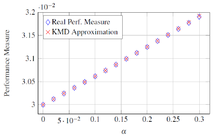
Figure 1: The performance measure of the network of two agents in Example 2 with the decaying parameter $\alpha$.

Remark 3

There is a limitation on the magnitude of the admissible initial conditions for the analysis conducted in the previous example. However, notice that this does not imply that it is a linear analysis since for any value of $\alpha$, the linearization matrix of $\mathcal{N}_{d}$ (with $k=1$) in Example 2 is the following matrix.

$$\vec{A}=\begin{bmatrix}1&-1\\ -1&1\end{bmatrix}+\vec{J}_{n}.$$

This means that the value of the performance measure computed using the linearized system for each value of decaying parameter $\alpha$ is only one value.

Example 3

The dynamics of oscillators have been observed to be closely related to the consensus dynamics. Kuramoto suggested a model of biological oscillation, in which each oscillator was connected to the other one; i.e., the topology was a complete graph. Instead the interactions can be limited over a certain graph jadbabaie2004stability , so the dynamics of agent $i$ can be represented as

$$\dot{x}_{i}=\omega_{i}+\sum_{\{i,j\}\in\mathcal{E}}w_{ij}(x_{j}-x_{i}),$$ (22)

where $\omega_{i}$ is the natural frequency and the coupling weight is

$$w_{ij}=K\frac{\sin(x_{i}-x_{j})}{x_{i}-x_{j}}.$$ (23)

When the agents are identical (i.e., when $\omega_{i}=\omega$ for some $\omega$), the change of variable $x_{i}\rightarrow x_{i}-\omega t$ induces a nonlinear consensus network that is

$$\dot{x}_{i}=\sum_{\{i,j\}\in\mathcal{E}}w_{ij}(x_{j}-x_{i}).$$ (24)

We proceed with a procedure for computation of performance measure similar to one introduced in Example 2. For two identical oscillators, with phases $\theta$ and $\gamma$, the dynamics are

$$\frac{d}{dt}\begin{bmatrix}\theta\\ \gamma\end{bmatrix}=K\,\begin{bmatrix}\sin(\gamma-\theta)\\ \sin(\theta-\gamma)\end{bmatrix},$$

Setting $k=1$, the disagreement Jacobian has eigenvalues $\lambda_{1}=-1$ and $\lambda_{2}=-2K$, with eigenfunctions $\phi_{1}$ and $\phi_{2}$, respectively. Again we only need the restriction of $\phi_{2}$ to $\mathbf{1}^{\perp}$. The equation (13) for these dynamics becomes

$$\begin{bmatrix}\partial\phi_{2}/\partial\theta\\ \partial\phi_{2}/\partial\gamma\end{bmatrix}^{T}{K\sin(\theta-\gamma)}{}\begin{bmatrix}1\\ -1\end{bmatrix}=-2K\phi_{2}.$$

The new variable $z:=\theta-\gamma$ creates a single ordinary differential equation that is

$$\frac{2\sin(z)}{d\phi_{2}}{dz}=2\phi_{2}\Rightarrow\frac{d\phi_{2}}{\phi_{2}}=\frac{1}{\sin(z)}dz,$$

which is integrated and manipulated to get

$$\phi_{2}=\pm\exp\left(-\ln(\cot(z/2))\right)=\pm\tan(z/2),$$

where we arbitrarily choose $+$. The eigenfunction $\phi_{2}$ is locally analytic around the origin for $|z|<\pi$. Restricting to $\mathbf{1}^{\perp}$, $\theta+\gamma=0$, so $z=2\theta$, hence

$$\phi_{2}(\theta,\gamma)=\phi_{2}(\theta)=\tan(\theta),$$

which helps write the components of $\vec{H}(\theta,\gamma)$ as $\vec{H}(\theta,\gamma)=\begin{bmatrix}\phi_{2}&0\end{bmatrix}^{T}$. First component of $\vec{H}^{-1}(\theta)$ satisfies $H_{1}^{-1}(\phi_{2}(\theta),0)=\theta.$ Hence, $H_{1}^{-1}(\theta,\gamma)=\arctan(\theta),$ which is again locally analytic for $|\theta|<1$ around zero.

We sample initial conditions from a uniform discrete random variable of $63$ equally distributed initial conditions in $\theta\in[0,\pi/5]$ (and $\gamma=-\theta$) with equal distance of $0.01$. We set $\vec{Q}=\vec{I}_{n}$ and use $17^{\text{th}}$ order Maclaurin series of eigenfunctions and $\vec{H}^{-1}(\theta)$ to assess $\rho(\mathcal{L})$. As shown in Fig. 2, we alter $K\in[0.2,4]$ and take a look at the values of the performance measure, once compared with the exact value of $\rho(\mathcal{L})$ (computed with the numerical integration of the trajectories). The numerical agreement in this experiment can be measured by the relative error of the performance using the KMD approximation, which was about $3\times 10^{-4}\%$ in the worst-case.

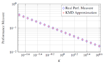
Figure 2: The performance measure of the Kuramoto model of two agents in Example 3 with the parameter $K$.

5 Sparse Polynomial Approximations

We have observed that any polynomial approximation to the inverse map of eigenfunctions $\vec{H}^{-1}(\vec{x})$ will result in the Koopman Mode Decompositions. In this section, first, we detail a general sparse approximation technique for multivariate interpolation. Then, we demonstrate how we can use this technique for the map of Koopman eigenfunctions $\vec{H}(\vec{x})$ as well as the inverse $\vec{H}^{-1}(\vec{x})$.

5.1 Smolyak-Collocation Method

To introduce the notion of sparsity for the approximation of both Koopman eigenfunctions and Koopman Mode Decomposition, we may use sparse functional approximation methods. The idea is that instead of searching for the approximant in the whole space of polynomials, the search is carried out over a nearly optimal sparse basis, called Smolyak basis. The output of the method would be a polynomial: the weighted sum of the tensor product of Chebyshev polynomials that are in the basis. Naturally, we choose the coefficients of the polynomial with respect to some error criterion. One way of doing so is collocation, where we enforce the approximant to (perhaps approximately) satisfy the governing equation of the problem at the given points of a grid, called Smolyak Sparse Grid. To describe this method, we need few basic tools (consult barthelmann2000high and malin2011solving for more details).

Definition 1 (Chebyshev Polynomials)

The sequence of the (scalar) Chebyshev polynomials of first kind $\{T_{i}(x)\}_{i=1,2,\dots}$ are initialized with $T_{1}(x)=1$ and $T_{2}(x)=x$ and recursively defined as follows.

$$T_{i+1}(x)=2xT_{i}(x)-T_{i-1}(x),\mbox{ for }i=2,3,\dots$$ (25)

Similarly, the Chebyshev polynomials of second kind $\{U_{i}(x)\}_{i=1,2,\dots}$ start with $U_{1}(x)=1$ and $U_{2}(x)=2x$, and then iteratively

$$U_{i+1}(x)=2xU_{i}(x)-U_{i-1}(x),\mbox{ for }i=2,3,\dots$$ (26)

We define the integer function $m(i):\mathbb{N}\rightarrow\mathbb{N}$ with $m(1)=1$ and for $i=2,3,\dots$, it is evaluated according to

$$m(i):=2^{i-1}+1.$$ (27)

We also define the sequence of sets $\{\mathcal{G}^{i}\}_{i=1,2,\dots}$ wherein, $\mathcal{G}^{1}=\{0\}$, and for $i=2,3,\dots$, it holds that $\mathcal{G}^{i}=\{\zeta_{1},\dots,\zeta_{i}\}\subset[-1,1]$, that is the set of the extrema of the Chebyshev polynomials with the components given by

$$\zeta_{j}:=-\cos\left(\frac{\pi(j-1)}{i-1}\right),\mbox{ for all }j\in\{1,\dots,i\}.$$ (28)

In the next definition, we use the multi-index notation $\mathbf{i}=(i_{1},\dots,i_{n}){\in\mathbb{N}^{n}}$ inducing $|\mathbf{i}|:=\sum_{k=1}^{n}i_{k}$.

Definition 2 (Smolyak Sparse Grid)

The Smolyak Sparse grid of $[-1,1]^{n}$ is a union of the Cartesian products of the form

$$\mathcal{H}^{n,\mu}:=\bigcup_{|\mathbf{i}|=n+\mu}\left(\mathcal{G}^{m(i_{1})}\times\dots\times\mathcal{G}^{m(i_{n})}\right),$$ (29)

where positive integer $\mu\in\mathbb{N}$ is the order of the grid.

Definition 3 (Smolyak Approximant Polynomial)

The Smolyak approximant to a function $f:[-1,1]^{n}\rightarrow\mathbb{R}$ is given by

$$\hat{f}^{n,\mu}(\vec{x}):={\sum}_{q\leq|\mathbf{i}|\leq n+\mu}(-1)^{n+\mu-|\mathbf{i}|}{n-1\choose n+\mu-|\mathbf{i}|}\mathrm{p}^{\mathbf{i}}{(\vec{x})},$$ (30)

with $q=\max(n,\mu+1)$ the tensor product polynomials for each multi-index $\mathbf{i}=(i_{1},\dots,i_{n})$ defined as

$$\mathrm{p}^{\mathbf{i}}(\vec{x}):=\sum_{l_{1}=1}^{m(i_{1})}\dots\sum_{l_{n}=1}^{m(i_{n})}\theta_{l_{1},\dots,l_{n}}T_{l_{1}}(x_{1})\dots T_{l_{n}}(x_{n}),$$ (31)

where $\theta_{l_{1},\dots,l_{n}}$ the coefficients that are to be determined.

To find the optimal vector of coefficients of ${\Theta}=\mathrm{vec}(\theta_{l_{1},\dots,l_{n}})\in\mathbb{R}^{m}$ for approximation of some function $f$ that is $C^{k}([-1,1]^{n})$, an error objective should be defined and minimized. One way is to consider the error function $E(f,\Theta):C^{k}([-1,1]^{n})\times\mathbb{R}^{n}\rightarrow\mathbb{R}_{+}$ to be

$$E(f,\Theta):= \underset{[-1,1]^{n}}{\int}\left|f(\vec{x})-f^{n,\mu}(\vec{x})\right|^{2}\prod_{\vec{y}\in\mathcal{H}^{n,\mu}}\delta(\vec{x}-\vec{y})~{}\mathrm{d}\vec{x}$$

$$=\sum_{\vec{y}\in\mathcal{H}^{n,\mu}}\left|f(\vec{y})-f^{n,\mu}(\vec{y})\right|^{2},$$

where $\delta$ is the Dirac’s delta function. This metric is certainly minimized (i.e., $E(f,\Theta)=0$) if $\Theta$ is chosen such that

$$f(\vec{x})=f^{n,\mu}(\vec{x})\mbox{ for all }\vec{x}\in\mathcal{H}^{n,\mu}.$$ (32)

This procedure is called collocation. A pivotal property of the overall method is that size of vector of coefficients $\Theta$ and the number of interpolation points is equal; i.e., $|\mathcal{H}^{n,\mu}|=|\Theta|=M.$ Therefore, enforcing equalities (32) constitutes of searching for the solution to $M$ equations involving $M$ unknown entries of $\Theta$. Once we evaluate the coefficients with the described scheme, the following error bound would hold, wherein the used functional norm $\|.\|:C^{k}\left({[-1,1]^{n}}\right)\rightarrow\mathbb{R}_{+}$ is defined as

$$\|f\|=\max\left\{{\left\|D^{i}f\right\|_{\infty}:~{}i=1,\dots,k}\right\}.$$ (33)

Theorem 5.1 ( Theorem 2 in barthelmann2000high )

Suppose that function $f(\vec{x}):[-1,1]^{n}\rightarrow\mathbb{R}$ is $C^{k}\left({[-1,1]^{n}}\right)$, together with a Smolyak approximant $\hat{f}^{n,\mu}(\vec{x})$ that interpolates $f$ on $\mathcal{H}^{n,\mu}$ with $|\mathcal{H}^{n,\mu}|=M$. Then, for some positive constant $c_{n,k}$, the error of the approximation is bounded according to

$$\left\|f-\hat{f}^{n,\mu}\right\|\leq c_{n,k}M^{-k}(\log M)^{(k+2)(n+1)+1}.$$ (34)

Each multi-index $\mathbf{i}$ in (30) induces a number of tensor product polynomials that are summed together as in (31). We gather the indices of all these tensor product polynomials in a set $\mathbf{L}^{n,\mu}$; i.e.,

$$\mathbf{L}^{n,\mu}:=\bigcup_{q\leq|\mathbf{i}|\leq n+\mu}\{(l_{1},\dots,l_{n}):l_{j}\leq m(i_{j})\}.$$ (35)

One can show that at the end of the day, the approximant constructed in (30) using the polynomials (31) boils down to the following simple representation

$$\hat{f}^{n,\mu}(\vec{x})=\sum_{\mathbf{l}_{i}=(l_{1}^{i},\dots,l_{n}^{i})\in\mathbf{L}^{n,\mu}}\Theta_{i}\mathrm{T}_{i}(\vec{x})=\sum_{i=1}^{M}\Theta_{i}\mathrm{T}_{i}(\vec{x}),$$ (36)

where $M=|\mathcal{H}^{n,\mu}|=|\mathbf{L}^{n,\mu}|$, and for $\mathbf{l}_{i}=(l_{1}^{i},\dots,l_{n}^{i})\in\mathbf{L}^{n,\mu}$, the coefficients ${\Theta}_{i}$ and polynomial terms are given by

$${\Theta}_{i}:=\theta_{l_{1}^{i},\dots,l_{n}^{i}},$$ (37)

$${\mathrm{T}}_{i}(\vec{x}):=T_{l_{1}^{i}}(x_{1})\dots T_{l_{n}^{i}}(x_{n}).$$ (38)

To compute the partial derivatives of approximation, we use the definitions of the Chebyshev polynomials to define

$${\mathrm{T}}_{i}^{j}(\vec{x}):=\left\{\begin{array}[]{ll}{\mathrm{T}}_{i}\cdot\dfrac{U_{l_{j}^{i}}(x_{j})}{T_{l_{j}^{i}}(x_{j})}&~{}~{}~{}~{}~{}l_{j}^{i}=2,\dots,n\vspace{2mm}\\ ~{}~{}~{}~{}~{}~{}~{}~{}~{}~{}0&~{}~{}~{}~{}~{}l_{j}^{i}=1\end{array}\right.,$$ (41)

This lets us write the partial derivatives of $\hat{f}^{n,\mu}$ in the compact form

$$\frac{\partial\hat{f}^{n,\mu}(\vec{x})}{\partial x_{j}}=\sum_{i=1}^{M}l_{j}^{i}{\Theta}_{i}\mathrm{T}_{i}^{j}(\vec{x}).$$ (42)

5.2 Sparse Approximation to Eigenfunctions

We denote the approximation to Koopman eigenfunction $\phi(\vec{x})$ by $\hat{\phi}(\vec{x})$. Substituting (36) and (42) into (13), we get the (approximate) equality

$$\sum_{j=1}^{n}\sum_{i=1}^{M}l_{j}^{i}{\Theta}_{i}\mathrm{T}_{i}^{j}(\vec{x})F_{j}(\vec{x})\approx\lambda\sum_{i=1}{M}{\Theta}_{i}\mathrm{T}_{i}(\vec{x}).$$

We change the order of summations to further obtain

$$\sum_{i=1}^{M}\left(\sum_{j=1}^{n}\left(l_{j}^{i}\mathrm{T}_{i}^{j}(\vec{x})F_{j}(\vec{x})\right)-\lambda\mathrm{T}_{i}(\vec{x})\right){\Theta}_{i}\approx 0.$$ (43)

We define and denote the vector of coefficients $\Theta\in\mathbb{R}^{M}$ by $\Theta:=[\Theta_{1},\dots,\Theta_{M}]^{T}.$ For a point in the grid $\vec{x}^{k}\in\mathcal{H}^{n,\mu}$, we may write the left hand side of (43) as

$$\mathcal{A}_{k}{\Theta}=\left[\mathcal{A}_{ki}\right]_{i=1,\dots,n}{\Theta},$$

where the entries of row vector $\mathcal{A}_{k}\in\mathbb{R}^{1\times M}$ can be computed from

$$\mathcal{A}_{ki}:=\sum_{j=1}^{n}\left(l_{j}^{i}\mathrm{T}_{i}^{j}(\vec{x}^{k})F_{j}(\vec{x}^{k})\right)-\lambda\mathrm{T}_{i}(\vec{x}^{k}),\text{ ~{}for all }i=1,\dots,M.$$

Repeating this for $M$ points in the Smolyak grid, the stacked left hand side of all equations becomes $\mathcal{A}\Theta$, where $\mathcal{A}\in\mathbb{R}^{M\times M}$ is given by

$$\mathcal{A}:=[\mathcal{A}_{1}^{T},\dots,\mathcal{A}_{M}^{T}]^{T}.$$ (44)

Ideally, $\mathcal{A}\Theta$ should be zero for an eigenfunction, however, if it is not possible, we would like to minimize an error function, which we choose to be

$$J(\Theta)=\|\mathcal{A}\Theta\|_{2}^{2}.$$ (45)

Now, because $\vec{A}$ may have repeated eigenvalues, we add a constraint that lets us derive multiple eigenfunctions corresponding to one eigenvalue. Consider the Koopman eigenfunction $\phi(\vec{x})$ with Koopman eigenvalue $\lambda$, which is the eigenvalue of the linearization matrix with a left eigenvector $\vec{R}=[\vec{r}_{1},\dots,\vec{r}_{n}]\in\mathbb{R}^{n\times n}$. We omit the index of the eigenvalues and eigenvectors in the following developments for simplicity and consider $\lambda$ to be associated with the eigenvector $\vec{r}\in\mathbb{R}^{n}$. We can show that with the fixed point at the origin,

$$\nabla\phi(\vec{x})|_{\vec{x}=\vec{0}}=\vec{r}.$$

Translating this for the approximant, for each $j=1,\dots,n$ we have

$$\frac{\partial\hat{\phi}(\vec{x})}{\partial x_{j}}|_{\vec{x}=\vec{0}}=\sum_{i=1}^{M}l_{j}^{i}{\Theta}_{i}\mathrm{T}_{i}^{j}(\vec{0})=\mathcal{B}_{j}\Theta=r_{j},$$

where the row vector $\mathcal{B}_{j}\in\mathbb{R}^{1\times M}$ has the components

$$\mathcal{B}_{ji}=l_{j}^{i}\mathrm{T}_{i}^{j}(\vec{0}),\text{~{}~{}for all }i=1,\dots,M.$$

The matrix form of this equality becomes

$$\mathcal{B}\Theta=\vec{r},$$ (46)

where the matrix $\mathcal{B}\in\mathbb{R}^{n\times M}$ is the result of stacking row vectors as

$$\mathcal{B}=\left[\mathcal{B}_{1}^{T},\dots,\mathcal{B}_{n}^{T}\right]^{T}.$$ (47)

Recall that our approximation requires $\hat{\phi}(\vec{0})=0$ to provide exponential convergence for the performance measure integrals (see Remark 2). This condition can be translated to single scalar equality

$$\mathcal{C}\Theta=0,$$ (48)

where $\mathcal{C}\in\mathbb{R}^{1\times M}$ is the row vector with elements

$$\mathcal{C}_{i}:=\mathrm{T}_{i}(\vec{0})\text{~{}~{}for all }i=1,\dots,M.$$

Now, we would like to minimize the error function defined by (45), while constraints (46) and (48) are satisfied. We define the optimization problem

$$\underset{\Theta\in\mathbb{R}^{m}}{\mathrm{minimize}}~{}~{}\|\mathcal{A}\Theta\|_{2}^{2},$$ (49)

$$\mathrm{subject~{}to}~{}\begin{bmatrix}\mathcal{B}\\ \mathcal{C}\end{bmatrix}\Theta=\begin{bmatrix}\vec{r}\\ 0\end{bmatrix}.$$

This program is equivalent to a Semi-Definite Program (SDP) and can be solved using the conventional convex programming such as CVX grant2010cvx .

5.3 Sparse Approximation to Koopman Mode Decomposition

In the previous subsection, we illustrated a way to find approximations to the Koopman eigenfunctions. Thus, the components of the map $\vec{H}(\vec{x})$ can be approximated. Here, following a similar approach, we seek approximations to the components of its inverse map $\vec{H}^{-1}(\vec{x})$. The very natural equation for component $H_{j}^{-1}(\vec{x})$ is

$$H_{j}^{-1}(\vec{H}(\vec{x}))=x_{j},~{}~{}\text{ for all }j=1,\dots,n.$$ (50)

We only have an approximation to $\vec{H}(\vec{x})$, namely $\hat{\vec{H}}(\vec{x})$, and we need approximations to $\hat{\vec{H}}^{-1}(\vec{x})$, namely $\hat{\vec{H}}^{-1}(\vec{x})$. Hence, we consider the approximate equality

$$\hat{H}_{j}^{-1}(\hat{\vec{H}}(\vec{x}))\approx x_{j},~{}~{}\text{ for all }j=1,\dots,n.$$ (51)

Again, following the spirit of the collocation method, for each point of the grid $\vec{x}^{k}\in\mathcal{H}^{n,\mu},$ we enforce this equation to hold. Suppose that we have found the series approximation to each components of $\vec{H}(\vec{x})$, denoted by $\hat{\vec{H}}(\vec{x})$. Moreover, we define

$$\vec{z}^{k}:=\hat{\vec{H}}(\vec{x}^{k}).$$ (52)

Then, we consider a Smolyak series representation for this function as

$$\hat{g}_{j}^{n,\mu}(\vec{z}^{k})=\sum_{i=1}^{M}{\Phi}_{i}^{j}\mathrm{T}_{i}(\vec{z}^{k}).$$ (53)

Similar to essence of the method that we discussed in the previous subsection, we define vector of coefficients $\Phi_{1}^{j}\in\mathbb{R}^{M}$ to be

$$\Phi^{j}:=\left[\Phi_{1}^{j},\dots,\Phi_{M}^{j}\right].$$

Inserting (53) into (50), we get

$$\mathcal{D}_{k}{\Phi}^{j}=\left[\mathcal{D}_{ki}\right]_{i=1,\dots,M}{\Phi}^{j}\approx x_{j}^{k},$$ (54)

where the components of row vector $\mathcal{D}_{k}\in\mathbb{R}^{1\times M}$ are

$$\mathcal{D}_{ki}:=\mathrm{T}_{i}(\vec{z}^{k}).$$ (55)

Concatenating these vectors and the right hand side scalars for each point in the grid (i.e., $M$ points), we may write these equations as

$$\mathcal{D}{\Phi}^{j}\approx\vec{X}_{j},$$ (56)

where matrix $\mathcal{D}\in\mathbb{R}^{M\times M}$ and vector $\vec{X}_{j}\in\mathbb{R}^{M}$ are given by

$$\mathcal{D}:=\left[\mathcal{D}_{1}^{T},\dots,\mathcal{D}_{M}^{T}\right]^{T},$$ (57)

$$\vec{X}_{j}:=\left[x_{j}^{1},\dots,x_{j}^{M}\right]^{T},$$ (58)

respectively. Again one hopes that (56) holds with a minimal error for each $j=1,\dots,n$. Therefore, we define the optimization problem

$$\underset{\Phi^{j}\in\mathbb{R}^{M}}{\mathrm{minimize}}~{}~{}\left\|\mathcal{D}\Phi^{j}-\vec{X}_{j}\right\|_{2}^{2}.$$ (59)

Note that matrix $\mathcal{D}$ is deliberately denoted without index $j$, because it is the same matrix for the optimization problem for each component $H_{j}^{-1}(\vec{x})$. The solution to this least-squares optimization problem is given by

$$\Phi^{j}=\mathcal{D}^{\dagger}\vec{X}_{j}~{}~{}\text{ for all }j=1,\dots,n.$$

We should repeat this for each component of $\vec{H}^{-1}(\vec{x})$. Putting the results in a matrix gives us

$$\Phi:=\left[\Phi^{1},\dots,\Phi^{n}\right].$$

Because the value of matrix $\mathcal{D}$ is shared between $M$ optimization problems defined by (59), by inspection, we find that

$$\Phi=\mathcal{D}^{\dagger}\vec{X}^{T},$$ (60)

where $\vec{X}\in\mathbb{R}^{n\times M}$ is the matrix containing the vector of all grid points. Now, we have a polynomial approximation to $\vec{H}^{-1}$, which would give us a Koopman Mode Decomposition.

5.4 Numerical Examples

In this section, we show that we may be able to effectively estimate the performance measure of nonlinear consensus networks with more than two subsystems. Note that in all cases, the real performance measure is calculated from the numerical solution of the network output followed by numerical integration.

Example 4 (Complete Graphs)

Using the described numerical approximation method, we estimate the performance measure for the nonlinear consensus network with exponentially decaying weights defined in (21). The corresponding linearized graph Laplacian corresponds to the undirected unweighted complete graph; i.e.

$$\vec{A}=-\mathcal{L}_{\mathcal{K}_{n}}=\vec{J}_{n}/n-\vec{I}_{n}.$$

We evaluate the performance measure from the KMD approximation based on the numerical integration of the solutions. The initial conditions are uniformly sampled random initial conditions from $[-1,1]^{n}$. The numerical values for data using Koopman approach have been obtained by implementation of the suggested numerical method with and the results are shown in Fig. 3. In this example, the error in the evaluated performance measure using our numerical method is less than $2\%$.

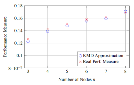
Figure 3: The performance measure of nonlinear consensus network with $\alpha=0.25$ and the graph at the linearized Laplacian of complete graph.

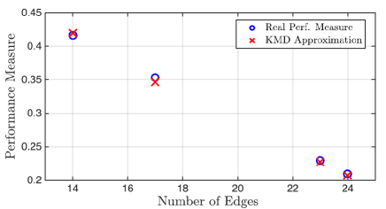
Figure 4: The performance measure of nonlinear consensus network with $n=8$, $\alpha=0.25$ and random graphs with different number of edges

Example 5 (Random Graphs)

We fix $n=8$ and create Erdős-Rényi graphs with different edges probabilities (and consequently, different edge numbers). Then, we consider again the exponentially decaying weights given by (21). The performance measures from Monte-Carlo simulations as well as the formula (using the method discussed in the previous sections) are also evaluated and illustrated in Fig. 4. The error of approximation, in this case, is less than $1.4\%$.

5.5 Comparison to Extended Dynamic Mode Decomposition

The numerical method explained in this section is related to the notion of Extended Dynamic Mode Decomposition (EDMD) williams2015data , which has been a promising procedure for extracting information about the Koopman spectrum of the dynamical system. In EDMD, to find a KMD for the flow of the dynamical system, one should first assume a rich enough dictionary of basis functions such that hopefully, the Koopman eigenfunctions lie in their span. Then, using the snapshots from the trajectory, one may find a truncated approximation to the Koopman operator and finite number of approximations to the Koopman eigenfunctions and their corresponding eigenvalues. Then, the solution to the dynamical system is approximated as a truncated KMD using those eigenvalues and eigenfunctions.

In the current settings, we know what are the eigenvalues and eigenfunctions that are required for representation of the flow of the nonlinear system. Hence, we do not need the first step of the EDMD for the computation of the (approximate) eigenvalues and eigenfunctions. In fact, we build the dictionary that one needs for EDMD based on the principal eigenfunctions in the map $\vec{H}(\vec{x})$.

On the other hand, the second step in both methods are connected in the spirit: In our approach, we find an approximation to map $\vec{H}^{-1}(\vec{x})$ using identity

$$\vec{H}^{-1}\left(\vec{H}(\vec{x})\right)=\vec{x}.$$

While in EDMD, the identity observable (i.e., $\mathbf{f}(\vec{x})\equiv\vec{x}$) has to be represented in terms of the basis functions in the dictionary. Then one is allowed to write down a KMD for the system dynamics as explained before.

6 Conclusion and Discussion

Koopman mode decomposition approaches hold promise for performance analysis and synthesis of nonlinear dynamical systems, that are of interest in various disciplines of engineering and control. The vital connection between the eigenspectrum of linearized dynamics and Koopman operator provides a closed form evaluation of the first moment of energy integral of the solutions, in terms of Koopman eigenvalues, eigenfunctions, and modes. The numerical approximation of KMD components is implemented by a scalable computational algorithm using sparse Smolyak grid with certifiable accuracy. Future directions include, but are not limited to the following directions: investigation and analysis of various performance metrics in nonlinear systems as extensions of linear control systems siami2016fundamental . Another research line regards dynamical systems with higher order integrators as well as a systemic performance-based network synthesis for optimal interactions among interconnected entities in the face of uncertain initial conditions or other structural parameters.

References

- (1) Abramowitz, M., Stegun, I.A., et al.: Handbook of mathematical functions. Applied mathematics series 55, 62 (1966)
- (2) Ajorlou, A., Momeni, A., Aghdam, A.G.: Sufficient conditions for the convergence of a class of nonlinear distributed consensus algorithms. Automatica 47(3), 625–629 (2011)
- (3) Ali, Q., Gageik, N., Montenegro, S.: A review on distributed control of cooperating mini uavs. International Journal of Artificial Intelligence & Applications 5(4), 1 (2014)
- (4) Arcak, M.: Passivity as a design tool for group coordination. IEEE Transactions on Automatic Control 52(8), 1380–1390 (2007)
- (5) de Badyn, M.H., Mesbahi, M.: Growing controllable networks via whiskering and submodular optimization. In: Decision and Control (CDC), 2016 IEEE 55th Conference on, pp. 867–872. IEEE (2016)
- (6) Bamieh, B., Jovanovic, M.R., Mitra, P., Patterson, S.: Coherence in large-scale networks: Dimension-dependent limitations of local feedback. IEEE Transactions on Automatic Control 57(9), 2235–2249 (2012)
- (7) Barthelmann, V., Novak, E., Ritter, K.: High dimensional polynomial interpolation on sparse grids. Advances in Computational Mathematics 12(4), 273–288 (2000)
- (8) Bassett, D.S., Bullmore, E.: Small-world brain networks. The neuroscientist 12(6), 512–523 (2006)
- (9) Beard, R.W., Lawton, J., Hadaegh, F.Y.: A coordination architecture for spacecraft formation control. IEEE Transactions on control systems technology 9(6), 777–790 (2001)
- (10) Budišić, M., Mohr, R., Mezić, I.: Applied koopmanism a. Chaos: An Interdisciplinary Journal of Nonlinear Science 22(4), 047,510 (2012)
- (11) Buzi, G., Topcu, U., Doyle, J.C.: Quantitative nonlinear analysis of autocatalytic pathways with applications to glycolysis. In: American Control Conference (ACC), 2010, pp. 3592–3597. IEEE (2010)
- (12) Charalambides, C.A.: Enumerative combinatorics. CRC Press (2002)
- (13) Chiang, H.D., Wu, F.F., Varaiya, P.P.: A bcu method for direct analysis of power system transient stability. IEEE Transactions on Power Systems 9(3), 1194–1208 (1994)
- (14) Cucker, F., Mordecki, E.: Flocking in noisy environments. arXiv preprint arXiv:0706.3343 (2007)
- (15) Cucker, F., Smale, S.: Emergent behavior in flocks. IEEE Transactions on Automatic Control 52(5), 852–862 (2007)
- (16) Cullen, H.F.: Introduction to General Topology. D C Heath & Co (1968)
- (17) Dai, R., , M.: Optimal topology design for dynamic networks. In: 2011 50th IEEE Conf. Decision Control / Euro. Control Conf., pp. 1280–1285. IEEE (2011)
- (18) Derriennic, M.M.: On multivariate approximation by bernstein-type polynomials. Journal of Approximation Theory 45, 155–166 (1985)
- (19) Dorfler, F., Bullo, F.: Synchronization and transient stability in power networks and nonuniform kuramoto oscillators. SIAM J. Control Optimization 50(3), 1616–1642 (2012)
- (20) Dörfler, F., Chertkov, M., Bullo, F.: Synchronization in complex oscillator networks and smart grids. Proceedings of the National Academy of Sciences 110(6), 2005–2010 (2013)
- (21) Grant, M., Boyd, S.: Cvx: Matlab software for disciplined convex programming, version 1.21 (2011). Available: cvxr. com/cvx (2010)
- (22) Jadbabaie, A., Lin, J., Morse, A.S.: Coordination of groups of mobile autonomous agents using nearest neighbor rules. IEEE Trans. Autom. Control 48(6), 988–1001 (2003)
- (23) Jadbabaie, A., Molavi, P., Sandroni, A., Tahbaz-Salehi, A.: Non-bayesian social learning. Games and Economic Behavior 76(1), 210–225 (2012)
- (24) Jadbabaie, A., Motee, N., Barahona, M.: On the stability of the kuramoto model of coupled nonlinear oscillators. In: Amer. Control Conf., Proc. 2004, vol. 5, pp. 4296–4301. IEEE (2004)
- (25) Kim, Y., , M.: On maximizing the second smallest eigenvalue of a state-dependent graph laplacian. In: American Control Conference, 2005. Proceedings of the 2005, pp. 99–103. IEEE (2005)
- (26) Kust, J., Brunton, S.L., Brunton, B.W., L., P.J.: Dynamic Mode Decomposition. Data-Driven Modeling of Complex Systems. OT149. SIAM (2016)
- (27) Lan, Y., Mezić, I.: Linearization in the large of nonlinear systems and koopman operator spectrum. Physica D: Nonlinear Phenomena 242(1), 42–53 (2013)
- (28) Leonard, N.E., Fiorelli, E.: Virtual leaders, artificial potentials and coordinated control of groups. In: Decision and Control, 2001. Proceedings of the 40th IEEE Conference on, vol. 3, pp. 2968–2973. IEEE (2001)
- (29) Lin, F., Fardad, M., Jovanović, M.R.: Design of optimal sparse feedback gains via the alternating direction method of multipliers. IEEE Transactions on Automatic Control 58(9), 2426–2431 (2013)
- (30) Malin, B.A., Krueger, D., Kubler, F.: Solving the multi-country real business cycle model using a smolyak-collocation method. Journal of Economic Dynamics and Control 35(2), 229–239 (2011)
- (31) Mauroy, A., Goncalves, J.: Koopman-based lifting techniques for nonlinear systems identification. arXiv preprint arXiv:1709.02003 (2017)
- (32) Mauroy, A., Mezić, I.: Global stability analysis using the eigenfunctions of the koopman operator. IEEE Transactions on Automatic Control 61(11), 3356–3369 (2016)
- (33) Mesbahi, M., Egerstedt, M.: Graph Theoretic Methods in Multiagent Networks. Princeton University Press (2010)
- (34) Moghaddam, S.H., Jovanović, M.R.: An interior point method for growing connected resistive networks. In: 2015 Amer. Control Conf., pp. 1223–1228 (2015)
- (35) Mousavi, H.K., Somarakis, C., Bahavarnia, M., Motee, N.: Performance bounds and optimal design of randomly switching linear consensus networks. In: American Control Conference (ACC), 2017, pp. 4347–4352. IEEE (2017)
- (36) Mousavi, H.K., Somarakis, C., Motee, N.: Koopman performance analysis of a class of nonlinear dynamical networks. In: Decision and Control (CDC), 2016 IEEE 55th Conference on, pp. 117–122. IEEE (2016)
- (37) Mousavi, H.K., Somarakis, C., Motee, N.: Spectral performance analysis and design for distributed control of multi-agent systems. In: Decision and Control (CDC), 2017 IEEE 56th Annual Conference on, pp. 2918–2923. IEEE (2017)
- (38) Olfati-Saber, R., Murray, R.M.: Consensus problems in networks of agents with switching topology and time-delays. IEEE Transactions on automatic control 49(9), 1520–1533 (2004)
- (39) Olshevsky, A., Tsitsiklis, J.N.: Convergence speed in distributed consensus and averaging. SIAM Journal on Control and Optimization 48(1), 33–55 (2009)
- (40) Papachristodoulou, A., Jadbabaie, A.: Synchonization in oscillator networks with heterogeneous delays, switching topologies and nonlinear dynamics. In: Decision and Control, 2006 45th IEEE Conference on, pp. 4307–4312. IEEE (2006)
- (41) Papachristodoulou, A., Jadbabaie, A., Munz, U.: Effects of delay in multi-agent consensus and oscillator synchronization. IEEE transactions on automatic control 55(6), 1471–1477 (2010)
- (42) Patterson, S., Bamieh, B.: Leader selection for optimal network coherence. In: Decision and Control (CDC), 2010 49th IEEE Conference on, pp. 2692–2697. IEEE (2010)
- (43) Perko, L.: Differential equations and dynamical systems, vol. 7. Springer Science & Business Media (2013)
- (44) van Riel, N.A., Sontag, E.D.: Parameter estimation in models combining signal transduction and metabolic pathways: the dependent input approach. IEE Proceedings-Systems Biology 153(4), 263–274 (2006)
- (45) Shilong, L., Mao, S.: Aerodynamic force and flow structures of two airfoils in flapping motions. Acta Mechanica Sinica 17(4), 310–331 (2001)
- (46) Siami, M., Motee, N.: On existence of hard limits in autocatalytic networks and their fundamental tradeoffs. IFAC Proceedings Volumes 45(26), 294–298 (2012)
- (47) Siami, M., Motee, N.: Performance analysis of linear consensus networks with structured stochastic disturbance inputs. In: 2015 Amer. Control Conf., pp. 4080–4085 (2015)
- (48) Siami, M., Motee, N.: Fundamental limits and tradeoffs on disturbance propagation in linear dynamical networks. IEEE Transactions on Automatic Control 61(12), 4055–4062 (2016)
- (49) Siami, M., Motee, N.: Growing linear dynamical networks endowed by spectral systemic performance measures. IEEE Transactions on Automatic Control 63(8) (2018)
- (50) Siami, M., Motee, N.: Network abstraction with guaranteed performance bounds. IEEE Transactions on Automatic Control (2018)
- (51) Somarakis, C., Baras, J.S.: Delay-independent convergence for linear consensus networks with applications to non-linear flocking systems. In: Submitted to the 12th IFAC Workshop on Time Delay Systems. Ann Arbor,MI,USA (2015)
- (52) Somarakis, C., Baras, J.S.: A simple proof of the continuous time linear consensus problem with applications in non-linear flocking networks. In: 14th European Control Conference. Linz,Austria (2015)
- (53) Somarakis, C., Ghaedsharaf, Y., Motee, N.: Time-delay origins of fundamental tradeoffs between risk of large fluctuations and network connectivity. arXiv preprint arXiv:1801.06856 (2018)
- (54) Susuki, Y., Mezic, I.: Nonlinear koopman modes and a precursor to power system swing instabilities. IEEE Transactions on Power Systems 27(3), 1182–1191 (2012)
- (55) Wang, P.K.: Navigation strategies for multiple autonomous mobile robots moving in formation. Journal of Field Robotics 8(2), 177–195 (1991)
- (56) Williams, M.O., Kevrekidis, I.G., Rowley, C.W.: A data–driven approximation of the koopman operator: Extending dynamic mode decomposition. Journal of Nonlinear Science 25(6), 1307–1346 (2015)