Orthogonal structure on a quadratic curve

Sheehan Olver Department of Mathematics
Imperial College
London
United Kingdom
s.olver@imperial.ac.uk
 and  Yuan Xu Department of Mathematics
University of Oregon
Eugene, Oregon 97403-1222.
yuan@uoregon.edu
Abstract.

Orthogonal polynomials on quadratic curves in the plane are studied. These include orthogonal polynomials on ellipses, parabolas, hyperbolas, and two lines. For an integral with respect to an appropriate weight function defined on any quadratic curve, an explicit basis of orthogonal polynomials is constructed in terms of two families of orthogonal polynomials in one variable. Convergence of the Fourier orthogonal expansions is also studied in each case. We discuss applications to the Fourier extension problem, interpolation of functions with singularities or near singularities, and the solution of Schrödinger’s equation with non-differentiable or nearly-non-differentiable potentials.

Key words and phrases:
Orthogonal polynomials, quadratic curve, plane, Fourier orthogonal expansions
2000 Mathematics Subject Classification:
42C05, 42C10, 33C50
The first author was supported in part by a Leverhulme Trust Research Project Grant and the second author was supported in part by NSF Grant DMS-1510296. Both authors would like to thank the Isaac Newton Institute for Mathematical Sciences for support and hospitality during the programmes “Approximation, sampling and compression in data science” and “Complex analysis: techniques, applications and computations” when work on this paper was undertaken. This work was supported by EPSRC grant number EP/R014604/1.

1. Introduction

The purpose of this work is to study orthogonal polynomials of two variables defined on a quadratic curve in the plane. Every quadratic curve in the plane satisfies an equation of the form

γ(x,y):=a1,1x2+2a1,2xy+a2,2y2+2a1,3x+2a2,3y+a3,3=0assign𝛾𝑥𝑦subscript𝑎11superscript𝑥22subscript𝑎12𝑥𝑦subscript𝑎22superscript𝑦22subscript𝑎13𝑥2subscript𝑎23𝑦subscript𝑎330\gamma(x,y):=a_{1,1}x^{2}+2a_{1,2}xy+a_{2,2}y^{2}+2a_{1,3}x+2a_{2,3}y+a_{3,3}=0

for some constants ai,ksubscript𝑎𝑖𝑘a_{i,k}. Let Ω=Ωγ:={(x,y):γ(x,y)=0}2ΩsubscriptΩ𝛾assignconditional-set𝑥𝑦𝛾𝑥𝑦0superscript2\Omega=\Omega_{\gamma}:=\{(x,y):\gamma(x,y)=0\}\subset{\mathbb{R}}^{2} be the trace of the curve in the plane. Let ϖ(x,y)italic-ϖ𝑥𝑦\varpi(x,y) be a nonnegative weight function defined on ΩΩ\Omega and satisfying Ωϖ(x,y)𝑑σ(x,y)>0subscriptΩitalic-ϖ𝑥𝑦differential-d𝜎𝑥𝑦0\int_{\Omega}\varpi(x,y)d\sigma(x,y)>0, where dσ𝑑𝜎d\sigma is the Lebesgue measure on the boundary ΩΩ\Omega. We consider the bilinear form defined by

(1.1) f,g=Ωf(x,y)g(x,y)ϖ(x,y)𝑑σ(x,y).𝑓𝑔subscriptΩ𝑓𝑥𝑦𝑔𝑥𝑦italic-ϖ𝑥𝑦differential-d𝜎𝑥𝑦{\langle}f,g{\rangle}=\int_{\Omega}f(x,y)g(x,y)\varpi(x,y)d\sigma(x,y).

Since f,g=0𝑓𝑔0{\langle}f,g{\rangle}=0 if either f𝑓f or g𝑔g belongs to the polynomial ideal γdelimited-⟨⟩𝛾\langle\gamma\rangle, it is an inner product only on the space [x,y]/γ𝑥𝑦delimited-⟨⟩𝛾{\mathbb{R}}[x,y]/\langle\gamma\rangle; that is, polynomials modulo the ideal γdelimited-⟨⟩𝛾{\langle}\gamma{\rangle}.

When γ(x,y)=1x2y2𝛾𝑥𝑦1superscript𝑥2superscript𝑦2\gamma(x,y)=1-x^{2}-y^{2}, so that ΩΩ\Omega is the unit circle, the orthogonal structure is well-understood. In particular, when ϖ(x,y)=1italic-ϖ𝑥𝑦1\varpi(x,y)=1, the orthogonal polynomials are spherical harmonics, which are homogeneous polynomials of two variables, their restriction on the circle are cos(nθ)𝑛𝜃\cos(n{\theta}) and sin(nθ)𝑛𝜃\sin(n{\theta}) where x=cosθ𝑥𝜃x=\cos{\theta} and y=sinθ𝑦𝜃y=\sin{\theta}, and the corresponding Fourier orthogonal expansions are the usual Fourier series. This case has served as the model for our recent study [9] of orthogonal polynomials on a wedge, defined as two line segments that share a common endpoint. In this paper we shall construct orthogonal polynomials for other quadratic curves.

Under an affine change of variables, quadratic curves in the plane are classified into five classes; three non-degenerate cases: ellipses, parabolas, and hyperbolas; and two degenerate cases: two intersecting real lines, and two parallel real lines. Since an affine change of variables does not change the degree of a polynomial in two variables, we only need to study orthogonal polynomials on a standard quadratic curve for each class of quadratic curves. Our choice of standard quadratic curves are the following:

  1.   (i)

    ellipse: x2+y2=1superscript𝑥2superscript𝑦21x^{2}+y^{2}=1;

  2.   (ii)

    parabola: y=x2𝑦superscript𝑥2y=x^{2};

  3.   (iii)

    hyperbola: x2y2=1superscript𝑥2superscript𝑦21x^{2}-y^{2}=1;

  4.   (iv)

    two intersection lines: x=0𝑥0x=0 and y=0𝑦0y=0; and,

  5.   (v)

    parallel lines: y=1𝑦1y=-1 and y=1𝑦1y=1.

As in the known cases of orthogonal polynomials on the unit circle and on a wedge, the space of orthogonal polynomials of degree n𝑛n has dimension 222 when n1𝑛1n\geq 1 for each quadratic curve. Assuming that ϖitalic-ϖ\varpi satisfies certain symmetry properties, the two-dimensional space of orthogonal polynomials on each quadratic curve can be expressed in terms of two different families of orthogonal polynomials in one variable, whose structure is well-understood. Furthermore, we shall relate the Fourier orthogonal expansions on the quadratic curve to those on the real line so that the convergence of the former can be deduced from the latter. Our approach will follow closely the development in [9] and relies heavily on symmetry of the domain and the weight function.

We consider three applications of the results. The first is usage in the Fourier extension problem, essentially rephrasing the known results of [7, 6] in terms of the orthogonal polynomials on quadratic curves. The second application is interpolation of functions on the real line with singularities of the form |x|𝑥|x|, x2+ϵ2superscript𝑥2superscriptitalic-ϵ2\sqrt{x^{2}+\epsilon^{2}}, and 1/x1𝑥1/x. For example, we consider functions on the interval [1,1]11[-1,1] of the form

f(x)=f(x2+ϵ2,x)𝑓𝑥𝑓superscript𝑥2superscriptitalic-ϵ2𝑥f(x)=f(\sqrt{x^{2}+\epsilon^{2}},x)

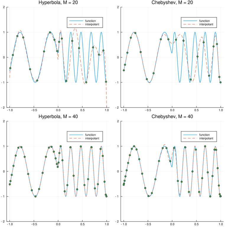
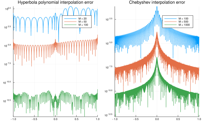
where f(x,y)𝑓𝑥𝑦f(x,y), defined on the hyperbola x2=y2+ϵ2superscript𝑥2superscript𝑦2superscriptitalic-ϵ2x^{2}=y^{2}+\epsilon^{2}, is entire in x𝑥x and y𝑦y. We will see that we can calculate the two-variable polynomial interpolant of f(x,y)𝑓𝑥𝑦f(x,y) using orthogonal polynomials via a suitably constructed quadrature rule. The resulting approximation converges super-exponentially fast, at a rate that is uniformly bounded as ϵ0italic-ϵ0\epsilon\rightarrow 0. This is in contrast to using only univariate orthogonal polynomials (e.g. an interpolant at Chebyshev points) whose convergence degenerates to algebraic as ϵ0italic-ϵ0\epsilon\rightarrow 0, as the convergence rate is dictated by the size of the Bernstein ellipse in the complex plane in which f(x)𝑓𝑥f(x) is analytic. The final application is solving Schrödinger’s equation when the potential is singular or nearly singular. In particular, we consider the equation

0.12u′′(t)+V(t)u=λusuperscript0.12superscript𝑢′′𝑡𝑉𝑡𝑢𝜆𝑢-0.1^{2}u^{\prime\prime}(t)+V(t)u=\lambda u

with V(t)=t2+ϵ2+(t0.1)2𝑉𝑡superscript𝑡2superscriptitalic-ϵ2superscript𝑡0.12V(t)=\sqrt{t^{2}+\epsilon^{2}}+(t-0.1)^{2} using Dirichlet conditions, showing that the eigenstates can be calculated robsutly for small ϵitalic-ϵ\epsilon by using a basis built out of orthogonal polynomials on the hyperbola.

The paper is organized as follows. The next section is preliminary, where we fix notations and lay down the groundwork. Orthogonal structure on the quadratic curves will be discussed in the next five sections, from Section 3 to Section 7, each standard quadratic curve is treated in its own section, in the order of (i) – (v). In Section 8 we show that interpolation with this basis is feasible via suitably constructed quadrature rules. Applications of the results are investigated in Section 9.

2. Preliminary

Any second degree curve in the plane satisfies an equation of the form

γ(x,y):=a1,1x2+2a1,2xy+a2,2y2+2a1,3x+2a2,3y+a3,3=0.assign𝛾𝑥𝑦subscript𝑎11superscript𝑥22subscript𝑎12𝑥𝑦subscript𝑎22superscript𝑦22subscript𝑎13𝑥2subscript𝑎23𝑦subscript𝑎330\gamma(x,y):=a_{1,1}x^{2}+2a_{1,2}xy+a_{2,2}y^{2}+2a_{1,3}x+2a_{2,3}y+a_{3,3}=0.

Let A=(ai,j)i,j=13𝐴superscriptsubscriptsubscript𝑎𝑖𝑗𝑖𝑗13A=(a_{i,j})_{i,j=1}^{3} with aj,i:=ai,jassignsubscript𝑎𝑗𝑖subscript𝑎𝑖𝑗a_{j,i}:=a_{i,j}. The curve is called non-degenerate if det(A)0𝐴0\det(A)\neq 0 and degenerate if det(A)=0𝐴0\det(A)=0. Let Δ:=a1,1a2,2a1,22assignΔsubscript𝑎11subscript𝑎22superscriptsubscript𝑎122\Delta:=a_{1,1}a_{2,2}-a_{1,2}^{2}. In the non-degenerate case, there are three classes of curves, ellipse (Δ>0Δ0\Delta>0), parabola (Δ=0Δ0\Delta=0), and hyperbola (Δ<0Δ0\Delta<0). In the degenerate case, there are two classes, two intersecting real lines (Δ>0Δ0\Delta>0) and two parallel lines (Δ=0Δ0\Delta=0). In the last case, we assume that the two parallel lines are distinct. If the two lines coincide, then an appropriate rotation and translation reduces the problem to the real line. Orthogonal polynomials on the real line have been studied extensively and are well-understood (cf. [13]).

Let Πn2superscriptsubscriptΠ𝑛2\Pi_{n}^{2} denote the space of polynomials of degree at most n𝑛n in two real variables. Let γ𝛾\gamma be a quadratic curve. With respect to the bilinear form (1.1) defined on γ𝛾{\gamma}, a polynomial PΠn2𝑃superscriptsubscriptΠ𝑛2P\in\Pi_{n}^{2} is called an orthogonal polynomial on the quadratic curve γ𝛾\gamma if P,Q=0𝑃𝑄0{\langle}P,Q{\rangle}=0 for all polynomials QΠm2𝑄superscriptsubscriptΠ𝑚2Q\in\Pi_{m}^{2} with m<n𝑚𝑛m<n and P,P>0𝑃𝑃0{\langle}P,P{\rangle}>0. Let n=n(ϖ)Πn2subscript𝑛subscript𝑛italic-ϖsuperscriptsubscriptΠ𝑛2{\mathcal{H}}_{n}={\mathcal{H}}_{n}(\varpi)\subset\Pi_{n}^{2} be the space of orthogonal polynomials of degree n𝑛n on the quadratic curve.

As mentioned in the introduction, we only need to consider a standard quadratic curve for each class. For each quadratic curve γ𝛾\gamma in (i) – (v), the bilinear form (1.1) defined on ΩγsubscriptΩ𝛾\Omega_{\gamma} is an inner product on the space [x,y]/γ𝑥𝑦delimited-⟨⟩𝛾{\mathbb{R}}[x,y]/\langle\gamma\rangle of polynomials modulo the ideal γdelimited-⟨⟩𝛾{\langle}\gamma{\rangle}. Using the explicit formula of γ𝛾\gamma for each standard form, it is easy to see that the following proposition holds.

Proposition 2.1.

The space nsubscript𝑛{\mathcal{H}}_{n} has dimension dim0=1dimensionsubscript01\dim{\mathcal{H}}_{0}=1 and dimn=2dimensionsubscript𝑛2\dim{\mathcal{H}}_{n}=2 for n1𝑛1n\geq 1.

An explicit basis for the space nsubscript𝑛{\mathcal{H}}_{n} will be constructed for each class of quadratic curves in Sections 3–7. Let {Yn,1,Yn,2}subscript𝑌𝑛1subscript𝑌𝑛2\{Y_{n,1},Y_{n,2}\} be an orthogonal basis of nsubscript𝑛{\mathcal{H}}_{n}. Then these two polynomials are orthogonal to all polynomials of lower degrees and they are orthogonal to each other. Let L2(ϖ,Ω)superscript𝐿2italic-ϖΩL^{2}(\varpi,\Omega) be the L2superscript𝐿2L^{2} space of Lebesgue integrable functions with finite norm f=f,f12norm𝑓superscript𝑓𝑓12\|f\|={\langle}f,f{\rangle}^{\frac{1}{2}}. For fL2(ϖ,Ω)𝑓superscript𝐿2italic-ϖΩf\in L^{2}(\varpi,\Omega) its Fourier orthogonal series is defined by

(2.1) f=f^0+n=1[f^n,1Yn,1+f^n,2Yn,2],𝑓subscript^𝑓0superscriptsubscript𝑛1delimited-[]subscript^𝑓𝑛1subscript𝑌𝑛1subscript^𝑓𝑛2subscript𝑌𝑛2f=\widehat{f}_{0}+\sum_{n=1}^{\infty}\left[\widehat{f}_{n,1}Y_{n,1}+\widehat{f}_{n,2}Y_{n,2}\right],

where

f^0:=f,11,1andf^n,i:=f,Yn,iYn,i,Yn,i,n1.formulae-sequenceassignsubscript^𝑓0𝑓111andformulae-sequenceassignsubscript^𝑓𝑛𝑖𝑓subscript𝑌𝑛𝑖subscript𝑌𝑛𝑖subscript𝑌𝑛𝑖𝑛1\widehat{f}_{0}:=\frac{{\langle}f,1{\rangle}}{{\langle}1,1{\rangle}}\quad\hbox{and}\quad\widehat{f}_{n,i}:=\frac{{\langle}f,Y_{n,i}{\rangle}}{{\langle}Y_{n,i},Y_{n,i}{\rangle}},\quad n\geq 1.

The partial sum operator Snfsubscript𝑆𝑛𝑓S_{n}f is defined by

(2.2) Snf:=f^0+k=1n[f^k,1Yk,1+f^k,2Yk,2].assignsubscript𝑆𝑛𝑓subscript^𝑓0superscriptsubscript𝑘1𝑛delimited-[]subscript^𝑓𝑘1subscript𝑌𝑘1subscript^𝑓𝑘2subscript𝑌𝑘2S_{n}f:=\widehat{f}_{0}+\sum_{k=1}^{n}\left[\widehat{f}_{k,1}Y_{k,1}+\widehat{f}_{k,2}Y_{k,2}\right].

We shall study the convergence of the Fourier orthogonal series on quadratic curves.

Our construction of orthogonal polynomials on the quadratic curves will heavilyuse orthogonal polynomials on the real line. Let w𝑤w be a nonnegative weight function on {\mathbb{R}}. We let pn(w)subscript𝑝𝑛𝑤p_{n}(w) denote an orthogonal polynomial of degree n𝑛n with respect to w𝑤w and let hn(w)subscript𝑛𝑤h_{n}(w) denote the norm square of pn(w)subscript𝑝𝑛𝑤p_{n}(w); more precisely,

pn(w;x)pm(w;x)w(x)𝑑x=hn(w)δm,n.subscriptsubscript𝑝𝑛𝑤𝑥subscript𝑝𝑚𝑤𝑥𝑤𝑥differential-d𝑥subscript𝑛𝑤subscript𝛿𝑚𝑛\int_{\mathbb{R}}p_{n}(w;x)p_{m}(w;x)w(x)dx=h_{n}(w)\delta_{m,n}.

Let L2(w)superscript𝐿2𝑤L^{2}(w) denote the L2superscript𝐿2L^{2} space with respect to w𝑤w on {\mathbb{R}}. The Fourier orthogonal series of fL2(w)𝑓superscript𝐿2𝑤f\in L^{2}(w) is defined by

(2.3) f=n=1f^n(w)pn(w)withf^n(w)=1hn(w)f(y)pn(w;y)w(y)𝑑y.formulae-sequence𝑓superscriptsubscript𝑛1subscript^𝑓𝑛𝑤subscript𝑝𝑛𝑤withsubscript^𝑓𝑛𝑤1subscript𝑛𝑤subscript𝑓𝑦subscript𝑝𝑛𝑤𝑦𝑤𝑦differential-d𝑦f=\sum_{n=1}^{\infty}\widehat{f}_{n}(w)p_{n}(w)\quad\hbox{with}\quad\widehat{f}_{n}(w)=\frac{1}{h_{n}(w)}\int_{\mathbb{R}}f(y)p_{n}(w;y)w(y)dy.

The Parseval identity implies that

fL2(w,[0,1])2=n=0|f^n(w)|2hn(w).superscriptsubscriptnorm𝑓superscript𝐿2𝑤012superscriptsubscript𝑛0superscriptsubscript^𝑓𝑛𝑤2subscript𝑛𝑤\|f\|_{L^{2}(w,[0,1])}^{2}=\sum_{n=0}^{\infty}\left|\widehat{f}_{n}(w)\right|^{2}h_{n}(w).

The n𝑛n-th partial sum of the Fourier orthogonal series with respect to w𝑤w is defined as

(2.4) sn(w;f)(x):=f^0(w)p0(w;x)+k=1nf^k(w)pk(w;x).assignsubscript𝑠𝑛𝑤𝑓𝑥subscript^𝑓0𝑤subscript𝑝0𝑤𝑥superscriptsubscript𝑘1𝑛subscript^𝑓𝑘𝑤subscript𝑝𝑘𝑤𝑥s_{n}(w;f)(x):=\widehat{f}_{0}(w)p_{0}(w;x)+\sum_{k=1}^{n}\widehat{f}_{k}(w)p_{k}(w;x).

Our study of the Fourier orthogonal series on a quadratic curve consists of reducing the problem to that of the Fourier orthogonal series on {\mathbb{R}}.

3. Orthogonal polynomials on an ellipse

Each ellipse can be transformed to the unit circle under an affine transform. Hence, we only need to consider the circle

Ω={(x,y):x2+y2=1}={(cosθ,sinθ):θ[0,2π]}.Ωconditional-set𝑥𝑦superscript𝑥2superscript𝑦21conditional-set𝜃𝜃𝜃02𝜋\Omega=\{(x,y):x^{2}+y^{2}=1\in{\mathbb{R}}\}=\{(\cos{\theta},\sin{\theta}):{\theta}\in[0,2\pi]\}.

Orthogonal polynomials on circles are well studied. However, it should be pointed out that we are considering them as real polynomials in two variables, which are distinct from the thoroughly studied Orthogonal Polynomials on the Unit Circle (OPUC) [11]. The latter are analytic polynomials in a complex z𝑧z variable and orthogonal with respect to an inner product defined on the unit circle in the complex plane. In our results, they are restrictions of homogeneous polynomials of two variables on the unit circle in 2superscript2{\mathbb{R}}^{2}. The result below is well–known, we include it here for completeness and also as an opening to our study for other quadratic curves.

Let w𝑤w be an even nonnegative weight function defined on [1,1]11[-1,1]. We consider the bilinear form defined by

f,g𝑓𝑔\displaystyle{\langle}f,g{\rangle} =ππf(cosθ,sinθ)g(cosθ,sinθ)w(cosθ)𝑑θabsentsuperscriptsubscript𝜋𝜋𝑓𝜃𝜃𝑔𝜃𝜃𝑤𝜃differential-d𝜃\displaystyle=\int_{-\pi}^{\pi}f(\cos{\theta},\sin{\theta})g(\cos{\theta},\sin{\theta})w(\cos{\theta})d{\theta}
=11[f(x,1x2)g(x,1x2)\displaystyle=\int_{-1}^{1}\Bigl{[}f(x,\sqrt{1-x^{2}})g(x,\sqrt{1-x^{2}})
(3.1) +f(x,1x2)g(x,1x2)]w(x)1x2dx\displaystyle\qquad+f(x,-\sqrt{1-x^{2}})g(x,-\sqrt{1-x^{2}})\Bigr{]}{w(x)\over\sqrt{1-x^{2}}}dx

which defines an inner product on the space [x,y]/x2+y21𝑥𝑦delimited-⟨⟩superscript𝑥2superscript𝑦21{\mathbb{R}}[x,y]/{\langle}x^{2}+y^{2}-1{\rangle}.

Let 𝒫nsubscript𝒫𝑛{\mathcal{P}}_{n} denote the space of homogeneous polynomials in two variables. Let n(ϖ)subscript𝑛italic-ϖ{\mathcal{H}}_{n}(\varpi) denote the space of orthogonal polynomials of degree n𝑛n with respect to this inner product.

Theorem 3.1.

Let w(t)𝑤𝑡w(t) be an even weight function defined on [1,1]11[-1,1]. Define w12(t)=(1t2)12w(t)subscript𝑤12𝑡superscript1superscript𝑡212𝑤𝑡w_{-\frac{1}{2}}(t)=(1-t^{2})^{-\frac{1}{2}}w(t) and w12(t)=(1t2)12w(t)subscript𝑤12𝑡superscript1superscript𝑡212𝑤𝑡w_{\frac{1}{2}}(t)=(1-t^{2})^{\frac{1}{2}}w(t). The polynomials

(3.2) Yn,1(x,y)=pn(w12;x)andYn,2(x,y)=ypn1(w12;x)formulae-sequencesubscript𝑌𝑛1𝑥𝑦subscript𝑝𝑛subscript𝑤12𝑥andsubscript𝑌𝑛2𝑥𝑦𝑦subscript𝑝𝑛1subscript𝑤12𝑥Y_{n,1}(x,y)=p_{n}(w_{-\frac{1}{2}};x)\quad\hbox{and}\quad Y_{n,2}(x,y)=yp_{n-1}(w_{\frac{1}{2}};x)

are homogeneous polynomials of degree n𝑛n in (x,y)𝑥𝑦(x,y) and they form an orthogonal basis of n(ϖ)subscript𝑛italic-ϖ{\mathcal{H}}_{n}(\varpi) for all n1𝑛1n\geq 1. Furthermore,

(3.3) Yn,1,Yn,1=2hn(w12)andYn,2,Yn,2=2hn1(w12).formulae-sequencesubscript𝑌𝑛1subscript𝑌𝑛12subscript𝑛subscript𝑤12andsubscript𝑌𝑛2subscript𝑌𝑛22subscript𝑛1subscript𝑤12{\langle}Y_{n,1},Y_{n,1}{\rangle}=2h_{n}(w_{-\frac{1}{2}})\quad\hbox{and}\quad{\langle}Y_{n,2},Y_{n,2}{\rangle}=2h_{n-1}(w_{\frac{1}{2}}).
Proof.

This result is known; see, for example, [3, Section 4.2]. We give an outline of the proof for completeness. Since w(t)𝑤𝑡w(t) is even, the polynomial pn(w;t)subscript𝑝𝑛𝑤𝑡p_{n}(w;t) is an even polynomial if n𝑛n is even and an odd polynomial if n𝑛n is odd. Consequently, it is easy to see that both Yn,1subscript𝑌𝑛1Y_{n,1} and Yn,2subscript𝑌𝑛2Y_{n,2} are homogeneous polynomials of degree n𝑛n in (x,y)𝑥𝑦(x,y). Since sinθ𝜃\sin{\theta} is odd, it follows readily that Yn,1,Ym,2=0subscript𝑌𝑛1subscript𝑌𝑚20{\langle}Y_{n,1},Y_{m,2}{\rangle}=0 for all n0𝑛0n\geq 0 and m1𝑚1m\geq 1. Moreover,

Yn,1,Yn,1subscript𝑌𝑛1subscript𝑌𝑛1\displaystyle{\langle}Y_{n,1},Y_{n,1}{\rangle} =211[pn(w12;t)]2w(t)1t2𝑑t=2hn(w12)absent2superscriptsubscript11superscriptdelimited-[]subscript𝑝𝑛subscript𝑤12𝑡2𝑤𝑡1superscript𝑡2differential-d𝑡2subscript𝑛subscript𝑤12\displaystyle=2\int_{-1}^{1}\left[p_{n}(w_{-\frac{1}{2}};t)\right]^{2}\frac{w(t)}{\sqrt{1-t^{2}}}dt=2h_{n}(w_{-\frac{1}{2}})

and, similarly, Yn,2,Yn,2=2hn1(w12)subscript𝑌𝑛2subscript𝑌𝑛22subscript𝑛1subscript𝑤12{\langle}Y_{n,2},Y_{n,2}{\rangle}=2h_{n-1}(w_{\frac{1}{2}}). ∎

The most well-known example are the spherical harmonics, for which w(t)=1𝑤𝑡1w(t)=1. The orthogonal polynomials are

Yn,1(x,y)subscript𝑌𝑛1𝑥𝑦\displaystyle Y_{n,1}(x,y) =cosnθ=Tn(x),absent𝑛𝜃subscript𝑇𝑛𝑥\displaystyle=\cos n{\theta}=T_{n}(x),
Yn,2(x,y)subscript𝑌𝑛2𝑥𝑦\displaystyle Y_{n,2}(x,y) =sinnθ=yUn1(x),absent𝑛𝜃𝑦subscript𝑈𝑛1𝑥\displaystyle=\sin n{\theta}=yU_{n-1}(x),

where Tn(t)subscript𝑇𝑛𝑡T_{n}(t) and Un(t)subscript𝑈𝑛𝑡U_{n}(t) are the Chebyshev polynomials of the first and the second kind, respectively. The restrictions of Yn,1subscript𝑌𝑛1Y_{n,1} and Yn,2subscript𝑌𝑛2Y_{n,2} to the circle are the eigenfunctions of d2/dθ2superscript𝑑2𝑑superscript𝜃2d^{2}/d{\theta}^{2} (which is the Laplace–Beltrami operator on the circle) in the sense that they satisfy u′′(θ)=nu(θ)superscript𝑢′′𝜃𝑛𝑢𝜃u^{\prime\prime}({\theta})=-nu({\theta}).

Another family of examples are hh-harmonics associated with the dihedral group Iksubscript𝐼𝑘I_{k} of k𝑘k-regular polygons in the plane (cf. [3, Section 7.6]). For k=1,2,𝑘12k=1,2,\ldots, the weight function in (3.1) is defined by

w(cosθ)=|sin(kθ)|2α|cos(kθ)|2β,α,β0.formulae-sequence𝑤𝜃superscript𝑘𝜃2𝛼superscript𝑘𝜃2𝛽𝛼𝛽0w(\cos{\theta})=|\sin(k{\theta})|^{2{\alpha}}|\cos(k{\theta})|^{2{\beta}},\qquad{\alpha},{\beta}\geq 0.

For each k𝑘k, the corresponding polynomials Yn,1subscript𝑌𝑛1Y_{n,1} and Yn,2subscript𝑌𝑛2Y_{n,2} are the eigenfunctions of a second order differential-difference operator on the circle [3, Section 7.6].

We can connect the Fourier orthogonal series on the circle to the Fourier orthogonal series in terms of w12subscript𝑤12w_{-\frac{1}{2}} and w12subscript𝑤12w_{\frac{1}{2}} on the interval [1,1]11[-1,1]. Recall the definition of partial sum operators defined in (2.2) and (2.4).

Theorem 3.2.

Let f𝑓f be a function defined on ΩΩ\Omega. Define

fe(x):=f(x,1x2)+f(x,1x2)2assignsubscript𝑓𝑒𝑥𝑓𝑥1superscript𝑥2𝑓𝑥1superscript𝑥22f_{e}(x):=\frac{f(x,\sqrt{1-x^{2}})+f(x,-\sqrt{1-x^{2}})}{2}

and

fo(x):=f(x,1x2)f(x,1x2)21x2.assignsubscript𝑓𝑜𝑥𝑓𝑥1superscript𝑥2𝑓𝑥1superscript𝑥221superscript𝑥2f_{o}(x):=\frac{f(x,\sqrt{1-x^{2}})-f(x,-\sqrt{1-x^{2}})}{2\sqrt{1-x^{2}}}.

Then

(3.4) Snf(x,y)=sn(w12;fe,x)+ysn1(w12;fo,x).subscript𝑆𝑛𝑓𝑥𝑦subscript𝑠𝑛subscript𝑤12subscript𝑓𝑒𝑥𝑦subscript𝑠𝑛1subscript𝑤12subscript𝑓𝑜𝑥\displaystyle S_{n}f(x,y)\,=s_{n}(w_{-\frac{1}{2}};f_{e},x)+ys_{n-1}(w_{\frac{1}{2}};f_{o},x).

In particular, if sn(w12;fe,x)fe(x)subscript𝑠𝑛subscript𝑤12subscript𝑓𝑒𝑥subscript𝑓𝑒𝑥s_{n}(w_{-\frac{1}{2}};f_{e},x)\to f_{e}(x) and sn1(w12;fo,x)fo(x)subscript𝑠𝑛1subscript𝑤12subscript𝑓𝑜𝑥subscript𝑓𝑜𝑥s_{n-1}(w_{\frac{1}{2}};f_{o},x)\to f_{o}(x) as n𝑛n\to\infty, then Snf(x,y)f(x,y)subscript𝑆𝑛𝑓𝑥𝑦𝑓𝑥𝑦S_{n}f(x,y)\to f(x,y) as n𝑛n\to\infty. Furthermore, if fL2(ϖ,Ω)𝑓superscript𝐿2italic-ϖΩf\in L^{2}(\varpi,\Omega), then

(3.5) fSn(f)L2(ϖ,Ω)2=superscriptsubscriptnorm𝑓subscript𝑆𝑛𝑓superscript𝐿2italic-ϖΩ2absent\displaystyle\|f-S_{n}(f)\|_{L^{2}(\varpi,\Omega)}^{2}= fesn(w12;fe)L2(w12)2+fosn1(w12;fo)L2(w12)2.superscriptsubscriptnormsubscript𝑓𝑒subscript𝑠𝑛subscript𝑤12subscript𝑓𝑒superscript𝐿2subscript𝑤122superscriptsubscriptnormsubscript𝑓𝑜subscript𝑠𝑛1subscript𝑤12subscript𝑓𝑜superscript𝐿2subscript𝑤122\displaystyle\,\|f_{e}-s_{n}(w_{-\frac{1}{2}};f_{e})\|_{L^{2}(w_{-\frac{1}{2}})}^{2}+\|f_{o}-s_{n-1}(w_{\frac{1}{2}};f_{o})\|_{L^{2}(w_{\frac{1}{2}})}^{2}.
Proof.

By the expression of Yn,1subscript𝑌𝑛1Y_{n,1} in (3.2),

f,Yn,1𝑓subscript𝑌𝑛1\displaystyle{\langle}f,Y_{n,1}{\rangle} =ππf(cosθ,sinθ)pn(w12;cosθ)w(cosθ)𝑑θabsentsuperscriptsubscript𝜋𝜋𝑓𝜃𝜃subscript𝑝𝑛subscript𝑤12𝜃𝑤𝜃differential-d𝜃\displaystyle\,=\int_{-\pi}^{\pi}f(\cos{\theta},\sin{\theta})p_{n}(w_{-\frac{1}{2}};\cos{\theta})w(\cos{\theta})d{\theta}
=0π[f(cosθ,sinθ)+f(cosθ,sinθ)]pn(w12;cosθ)w(cosθ)𝑑θabsentsuperscriptsubscript0𝜋delimited-[]𝑓𝜃𝜃𝑓𝜃𝜃subscript𝑝𝑛subscript𝑤12𝜃𝑤𝜃differential-d𝜃\displaystyle\,=\int_{0}^{\pi}\left[f(\cos{\theta},\sin{\theta})+f(\cos{\theta},-\sin{\theta})\right]p_{n}(w_{-\frac{1}{2}};\cos{\theta})w(\cos{\theta})d{\theta}
=211fe(t)pn(w12;t)w12(t)𝑑t=2fe,pn(w12)L2(w12).absent2superscriptsubscript11subscript𝑓𝑒𝑡subscript𝑝𝑛subscript𝑤12𝑡subscript𝑤12𝑡differential-d𝑡2subscriptsubscript𝑓𝑒subscript𝑝𝑛subscript𝑤12superscript𝐿2subscript𝑤12\displaystyle\,=2\int_{-1}^{1}f_{e}(t)p_{n}(w_{-\frac{1}{2}};t)w_{-\frac{1}{2}}(t)dt=2{\langle}f_{e},p_{n}(w_{-\frac{1}{2}}){\rangle}_{L^{2}(w_{-\frac{1}{2}})}.

Similarly, by the expression of Yn,2subscript𝑌𝑛2Y_{n,2} in (3.2),

f,Yn,2𝑓subscript𝑌𝑛2\displaystyle{\langle}f,Y_{n,2}{\rangle} =0π[f(cosθ,sinθ)f(cosθ,sinθ)]sinθpn1(w12;cosθ)w(cosθ)𝑑θabsentsuperscriptsubscript0𝜋delimited-[]𝑓𝜃𝜃𝑓𝜃𝜃𝜃subscript𝑝𝑛1subscript𝑤12𝜃𝑤𝜃differential-d𝜃\displaystyle\,=\int_{0}^{\pi}\left[f(\cos{\theta},\sin{\theta})-f(\cos{\theta},-\sin{\theta})\right]\sin{\theta}p_{n-1}(w_{\frac{1}{2}};\cos{\theta})w(\cos{\theta})d{\theta}
=0πf(cosθ,sinθ)f(cosθ,sinθ)sinθsin2θpn1(w12;cosθ)w(cosθ)𝑑θabsentsuperscriptsubscript0𝜋𝑓𝜃𝜃𝑓𝜃𝜃𝜃superscript2𝜃subscript𝑝𝑛1subscript𝑤12𝜃𝑤𝜃differential-d𝜃\displaystyle\,=\int_{0}^{\pi}\frac{f(\cos{\theta},\sin{\theta})-f(\cos{\theta},-\sin{\theta})}{\sin{\theta}}\sin^{2}{\theta}p_{n-1}(w_{\frac{1}{2}};\cos{\theta})w(\cos{\theta})d{\theta}
=211fo(t)pn1(w12;t)w12(t)𝑑t=2fo,pn1(w12)L2(w12).absent2superscriptsubscript11subscript𝑓𝑜𝑡subscript𝑝𝑛1subscript𝑤12𝑡subscript𝑤12𝑡differential-d𝑡2subscriptsubscript𝑓𝑜subscript𝑝𝑛1subscript𝑤12superscript𝐿2subscript𝑤12\displaystyle\,=2\int_{-1}^{1}f_{o}(t)p_{n-1}(w_{\frac{1}{2}};t)w_{\frac{1}{2}}(t)dt=2{\langle}f_{o},p_{n-1}(w_{\frac{1}{2}}){\rangle}_{L^{2}(w_{\frac{1}{2}})}.

Consequently, by (3.3), we obtain

f^n,1=fe,pn(w12)L2(w12)hn(w12)=fe^n(w12),f^n,2=fo,pn1(w12)L2(w12)hn1(w12)=fo^n1(w12)formulae-sequencesubscript^𝑓𝑛1subscriptsubscript𝑓𝑒subscript𝑝𝑛subscript𝑤12superscript𝐿2subscript𝑤12subscript𝑛subscript𝑤12subscript^subscript𝑓𝑒𝑛subscript𝑤12subscript^𝑓𝑛2subscriptsubscript𝑓𝑜subscript𝑝𝑛1subscript𝑤12superscript𝐿2subscript𝑤12subscript𝑛1subscript𝑤12subscript^subscript𝑓𝑜𝑛1subscript𝑤12\displaystyle\widehat{f}_{n,1}=\frac{{\langle}f_{e},p_{n}(w_{-\frac{1}{2}}){\rangle}_{L^{2}(w_{-\frac{1}{2}})}}{h_{n}(w_{-\frac{1}{2}})}=\widehat{f_{e}}_{n}(w_{-\frac{1}{2}}),\,\,\widehat{f}_{n,2}=\frac{{\langle}f_{o},p_{n-1}(w_{\frac{1}{2}}){\rangle}_{L^{2}(w_{\frac{1}{2}})}}{h_{n-1}(w_{\frac{1}{2}})}=\widehat{f_{o}}_{n-1}(w_{\frac{1}{2}})

in the notation of (2.3). Hence, (3.4) follows readily from the definition of the partial sum operators in (2.2).

With y=1x2𝑦1superscript𝑥2y=\sqrt{1-x^{2}}, we see that f(x,y)=fe(x)+yfo(x)𝑓𝑥𝑦subscript𝑓𝑒𝑥𝑦subscript𝑓𝑜𝑥f(x,y)=f_{e}(x)+yf_{o}(x). It follows that

f(x,y)Snf(x,y)=fe(x)sn(w12;fe,x)+y(fo(x)sn1(w12;fo,x)).𝑓𝑥𝑦subscript𝑆𝑛𝑓𝑥𝑦subscript𝑓𝑒𝑥subscript𝑠𝑛subscript𝑤12subscript𝑓𝑒𝑥𝑦subscript𝑓𝑜𝑥subscript𝑠𝑛1subscript𝑤12subscript𝑓𝑜𝑥\displaystyle f(x,y)-S_{n}f(x,y)=f_{e}(x)-s_{n}(w_{-\frac{1}{2}};f_{e},x)+y\left(f_{o}(x)-s_{n-1}(w_{\frac{1}{2}};f_{o},x)\right).

Consequently, the convergence of Snfsubscript𝑆𝑛𝑓S_{n}f follows form that of sn(w12;fe)subscript𝑠𝑛subscript𝑤12subscript𝑓𝑒s_{n}(w_{-\frac{1}{2}};f_{e}) and sn1(w12;fo)subscript𝑠𝑛1subscript𝑤12subscript𝑓𝑜s_{n-1}(w_{\frac{1}{2}};f_{o}). Finally, let F=fesn(w12;fe)𝐹subscript𝑓𝑒subscript𝑠𝑛subscript𝑤12subscript𝑓𝑒F=f_{e}-s_{n}(w_{-\frac{1}{2}};f_{e}) and G=fosn1(w12;fo)𝐺subscript𝑓𝑜subscript𝑠𝑛1subscript𝑤12subscript𝑓𝑜G=f_{o}-s_{n-1}(w_{\frac{1}{2}};f_{o}). Then the last displayed identity shows that

fSnfL2(ϖ,Ω)2=superscriptsubscriptnorm𝑓subscript𝑆𝑛𝑓superscript𝐿2italic-ϖΩ2absent\displaystyle\|f-S_{n}f\|_{L^{2}(\varpi,\Omega)}^{2}= ππ|F(cosθ)+sinθG(cosθ)|2w(cosθ)𝑑θsuperscriptsubscript𝜋𝜋superscript𝐹𝜃𝜃𝐺𝜃2𝑤𝜃differential-d𝜃\displaystyle\,\int_{-\pi}^{\pi}|F(\cos{\theta})+\sin{\theta}G(\cos{\theta})|^{2}w(\cos{\theta})d{\theta}
=\displaystyle= ππ(|F(cosθ)|2+|sinθG(cosθ)|2)w(cosθ)𝑑θsuperscriptsubscript𝜋𝜋superscript𝐹𝜃2superscript𝜃𝐺𝜃2𝑤𝜃differential-d𝜃\displaystyle\,\int_{-\pi}^{\pi}\left(|F(\cos{\theta})|^{2}+|\sin{\theta}G(\cos{\theta})|^{2}\right)w(\cos{\theta})d{\theta}
=\displaystyle= 11|F(t)|2w12(t)𝑑t+11|G(t)|2w12(t)𝑑t,superscriptsubscript11superscript𝐹𝑡2subscript𝑤12𝑡differential-d𝑡superscriptsubscript11superscript𝐺𝑡2subscript𝑤12𝑡differential-d𝑡\displaystyle\int_{-1}^{1}|F(t)|^{2}w_{-\frac{1}{2}}(t)dt+\int_{-1}^{1}|G(t)|^{2}w_{\frac{1}{2}}(t)dt,

where we have used the fact that the integral of sinθF(cosθ)G(cosθ)𝜃𝐹𝜃𝐺𝜃\sin{\theta}F(\cos{\theta})G(\cos\theta) is zero in the second step. This gives (3.5) and completes the proof. ∎

This theorem is also known but probably not stated in this precise form. When f𝑓f is chosen as f(x,y)=g(cosθ)𝑓𝑥𝑦𝑔𝜃f(x,y)=g(\cos{\theta}), then the Fourier orthogonal series of f𝑓f becomes the Fourier orthogonal series of g𝑔g in L2(w;[1,1])superscript𝐿2𝑤11L^{2}(w;[-1,1]). For the classical Fourier series, it is the familiar fact that the Fourier series of f(cosθ)𝑓𝜃f(\cos{\theta}) is the Fourier cosine series of f(t)𝑓𝑡f(t). We choose to give a complete proof here since it is the harbinger of what will come for other quadratic curves.

4. Orthogonal polynomials on a parabola

Under an affine transform, we only need to consider the parabola defined by

y=x2orΩ={(x,y):y=x2,x},formulae-sequence𝑦superscript𝑥2orΩconditional-set𝑥𝑦formulae-sequence𝑦superscript𝑥2𝑥y=x^{2}\qquad\hbox{or}\qquad\Omega=\{(x,y):y=x^{2},\,x\in{\mathbb{R}}\},

and consider even weights ϖ(x,y)=ϖ(x,y)italic-ϖ𝑥𝑦italic-ϖ𝑥𝑦\varpi(x,y)=\varpi(-x,y). Since y=x2𝑦superscript𝑥2y=x^{2}, we can write ϖ(x,y)=w(x2)italic-ϖ𝑥𝑦𝑤superscript𝑥2\varpi(x,y)=w(x^{2}) for a weight function w𝑤w on +=[0,+)subscript0{\mathbb{R}}_{+}=[0,+\infty), so that the bilinear form becomes

(4.1) f,g=f(x,x2)g(x,x2)w(x2)𝑑x,𝑓𝑔subscript𝑓𝑥superscript𝑥2𝑔𝑥superscript𝑥2𝑤superscript𝑥2differential-d𝑥{\langle}f,g{\rangle}=\int_{\mathbb{R}}f(x,x^{2})g(x,x^{2})w(x^{2})dx,

which defines an inner product on the space [x,y]/yx2𝑥𝑦delimited-⟨⟩𝑦superscript𝑥2{\mathbb{R}}[x,y]/{\langle}y-x^{2}{\rangle}.

4.1. Orthogonal polynomials

Let n(ϖ)subscript𝑛italic-ϖ{\mathcal{H}}_{n}(\varpi) denote the space of orthogonal polynomials of degree n𝑛n with respect to the inner product (4.1).

Theorem 4.1.

Let w𝑤w be a weight function defined on +subscript{\mathbb{R}}_{+}. Define w12(t):=t12w(t)assignsubscript𝑤12𝑡superscript𝑡12𝑤𝑡w_{-\frac{1}{2}}(t):=t^{-\frac{1}{2}}w(t) and w12(t):=t12w(t)assignsubscript𝑤12𝑡superscript𝑡12𝑤𝑡w_{\frac{1}{2}}(t):=t^{\frac{1}{2}}w(t). Then the polynomials

(4.2) Yn,1(x,y)=pn(w12;y)andYn,2(x,y)=xpn1(w12;y)formulae-sequencesubscript𝑌𝑛1𝑥𝑦subscript𝑝𝑛subscript𝑤12𝑦andsubscript𝑌𝑛2𝑥𝑦𝑥subscript𝑝𝑛1subscript𝑤12𝑦Y_{n,1}(x,y)=p_{n}(w_{-\frac{1}{2}};y)\quad\hbox{and}\quad Y_{n,2}(x,y)=xp_{n-1}(w_{\frac{1}{2}};y)

form an orthogonal basis of n(ϖ)subscript𝑛italic-ϖ{\mathcal{H}}_{n}(\varpi) for n1𝑛1n\geq 1. Furthermore,

(4.3) Yn,1,Yn,1=hn(w12)andYn,2,Yn,2=hn1(w12).formulae-sequencesubscript𝑌𝑛1subscript𝑌𝑛1subscript𝑛subscript𝑤12andsubscript𝑌𝑛2subscript𝑌𝑛2subscript𝑛1subscript𝑤12{\langle}Y_{n,1},Y_{n,1}{\rangle}=h_{n}(w_{-\frac{1}{2}})\quad\hbox{and}\quad{\langle}Y_{n,2},Y_{n,2}{\rangle}=h_{n-1}(w_{\frac{1}{2}}).
Proof.

For n0𝑛0n\geq 0 and m0𝑚0m\geq 0,

Yn,1,Ym,2=subscript𝑌𝑛1subscript𝑌𝑚2absent\displaystyle{\langle}Y_{n,1},Y_{m,2}{\rangle}=\, Yn,1(x,x2)Ym,2(x,x2)w(x2)𝑑xsubscriptsubscript𝑌𝑛1𝑥superscript𝑥2subscript𝑌𝑚2𝑥superscript𝑥2𝑤superscript𝑥2differential-d𝑥\displaystyle\int_{\mathbb{R}}Y_{n,1}(x,x^{2})Y_{m,2}(x,x^{2})w(x^{2})dx
=\displaystyle=\, xpn(w12,x2)pn1(w12;x2)w(x2)𝑑x=0subscript𝑥subscript𝑝𝑛subscript𝑤12superscript𝑥2subscript𝑝𝑛1subscript𝑤12superscript𝑥2𝑤superscript𝑥2differential-d𝑥0\displaystyle\int_{\mathbb{R}}xp_{n}(w_{-\frac{1}{2}},x^{2})p_{n-1}(w_{\frac{1}{2}};x^{2})w(x^{2})dx=0

since the integrand is odd. For n,m0𝑛𝑚subscript0n,m\in{\mathbb{N}}_{0},

Yn,1,Ym,1=subscript𝑌𝑛1subscript𝑌𝑚1absent\displaystyle{\langle}Y_{n,1},Y_{m,1}{\rangle}=\, pn(w12;x2)pm(w12;x2)w(x2)𝑑xsubscriptsubscript𝑝𝑛subscript𝑤12superscript𝑥2subscript𝑝𝑚subscript𝑤12superscript𝑥2𝑤superscript𝑥2differential-d𝑥\displaystyle\int_{\mathbb{R}}p_{n}(w_{-\frac{1}{2}};x^{2})p_{m}(w_{-\frac{1}{2}};x^{2})w(x^{2})dx
=\displaystyle=\, 20pn(w12;x2)pm(w12;x2)w(x2)𝑑x2superscriptsubscript0subscript𝑝𝑛subscript𝑤12superscript𝑥2subscript𝑝𝑚subscript𝑤12superscript𝑥2𝑤superscript𝑥2differential-d𝑥\displaystyle 2\int_{0}^{\infty}p_{n}(w_{-\frac{1}{2}};x^{2})p_{m}(w_{-\frac{1}{2}};x^{2})w(x^{2})dx
=\displaystyle=\, 0pn(w12;t)pm(w12;t)t12w(t)𝑑t=hn(w12)δn,m.superscriptsubscript0subscript𝑝𝑛subscript𝑤12𝑡subscript𝑝𝑚subscript𝑤12𝑡superscript𝑡12𝑤𝑡differential-d𝑡subscript𝑛subscript𝑤12subscript𝛿𝑛𝑚\displaystyle\int_{0}^{\infty}p_{n}(w_{-\frac{1}{2}};t)p_{m}(w_{-\frac{1}{2}};t)t^{-\frac{1}{2}}w(t)dt=h_{n}(w_{-\frac{1}{2}})\delta_{n,m}.

Similarly, for n,m𝑛𝑚n,m\in{\mathbb{N}},

Yn,2,Ym,2=subscript𝑌𝑛2subscript𝑌𝑚2absent\displaystyle{\langle}Y_{n,2},Y_{m,2}{\rangle}=\, x2pn1(w12;x2)pm1(w12;x2)w(x2)𝑑xsubscriptsuperscript𝑥2subscript𝑝𝑛1subscript𝑤12superscript𝑥2subscript𝑝𝑚1subscript𝑤12superscript𝑥2𝑤superscript𝑥2differential-d𝑥\displaystyle\int_{\mathbb{R}}x^{2}p_{n-1}(w_{\frac{1}{2}};x^{2})p_{m-1}(w_{\frac{1}{2}};x^{2})w(x^{2})dx
=\displaystyle=\, 0pn1(w12;t)pm1(w12;t)t12w(t)𝑑t=hn1(w12)δn,m.superscriptsubscript0subscript𝑝𝑛1subscript𝑤12𝑡subscript𝑝𝑚1subscript𝑤12𝑡superscript𝑡12𝑤𝑡differential-d𝑡subscript𝑛1subscript𝑤12subscript𝛿𝑛𝑚\displaystyle\int_{0}^{\infty}p_{n-1}(w_{\frac{1}{2}};t)p_{m-1}(w_{\frac{1}{2}};t)t^{\frac{1}{2}}w(t)dt=h_{n-1}(w_{\frac{1}{2}})\delta_{n,m}.

Since it is evident that Yn,1subscript𝑌𝑛1Y_{n,1} and Yn,2subscript𝑌𝑛2Y_{n,2} are polynomials of degree n𝑛n in two variables, we see that they form an orthogonal basis for n(ϖ)subscript𝑛italic-ϖ{\mathcal{H}}_{n}(\varpi). ∎

We consider two examples of classical orthogonal polynomials. Our first example is on the entire parabola {(x,y):y=x2,x}conditional-set𝑥𝑦formulae-sequence𝑦superscript𝑥2𝑥\{(x,y):y=x^{2},x\in{\mathbb{R}}\} with the Hermite weight w(t)=et2𝑤𝑡superscript𝑒superscript𝑡2w(t)=e^{-t^{2}}. Let Lnαsuperscriptsubscript𝐿𝑛𝛼L_{n}^{\alpha} denote the Laguerre polynomials, which are orthogonal with respect to xαexsuperscript𝑥𝛼superscript𝑒𝑥x^{\alpha}e^{-x} on +subscript{\mathbb{R}}_{+}.

Proposition 4.2.

For the inner product with respect to the Hermite weight

f,g=f(x,x2)g(x,x2)ex2𝑑x𝑓𝑔subscript𝑓𝑥superscript𝑥2𝑔𝑥superscript𝑥2superscript𝑒superscript𝑥2differential-d𝑥{\langle}f,g{\rangle}=\int_{{\mathbb{R}}}f(x,x^{2})g(x,x^{2})e^{-x^{2}}dx

and n1𝑛1n\geq 1, an orthogonal basis of nsubscript𝑛{\mathcal{H}}_{n} is given by the polynomials

Yn,1(x,y)=Ln12(y)andYn,2(x,y)=xLn112(y).formulae-sequencesubscript𝑌𝑛1𝑥𝑦superscriptsubscript𝐿𝑛12𝑦andsubscript𝑌𝑛2𝑥𝑦𝑥superscriptsubscript𝐿𝑛112𝑦Y_{n,1}(x,y)=L_{n}^{-\frac{1}{2}}(y)\quad\hbox{and}\quad Y_{n,2}(x,y)=xL_{n-1}^{\frac{1}{2}}(y).

Furthermore, they are the eigenfunctions of a second order differential operator; more precisely, Yn,1subscript𝑌𝑛1Y_{n,1} and Yn,2subscript𝑌𝑛2Y_{n,2} satisfy the equation

(4.4) u:=xxyu+yyyu+(12y)yuxxu=nu.assign𝑢𝑥subscript𝑥𝑦𝑢𝑦subscript𝑦𝑦𝑢12𝑦subscript𝑦𝑢𝑥subscript𝑥𝑢𝑛𝑢{\mathcal{L}}u:=x\partial_{xy}u+y\partial_{yy}u+(\tfrac{1}{2}-y)\partial_{y}u-x\partial_{x}u=-nu.
Proof.

We only need to verify the differential equations. The Laguerre polynomial v(y)=Lnα(y)𝑣𝑦superscriptsubscript𝐿𝑛𝛼𝑦v(y)=L_{n}^{\alpha}(y) satisfies the equation

v′′+(α+1y)v=nv.superscript𝑣′′𝛼1𝑦superscript𝑣𝑛𝑣v^{\prime\prime}+({\alpha}+1-y)v^{\prime}=-nv.

For u=Yn,1𝑢subscript𝑌𝑛1u=Y_{n,1}, we have xu=0subscript𝑥𝑢0\partial_{x}u=0 and it is easy to see that (4.4) becomes the differential equation for v(y)=Ln12(y)𝑣𝑦superscriptsubscript𝐿𝑛12𝑦v(y)=L_{n}^{-\frac{1}{2}}(y). For u=Yn,2𝑢subscript𝑌𝑛2u=Y_{n,2}, we write u(x,y)=xv(y)𝑢𝑥𝑦𝑥𝑣𝑦u(x,y)=xv(y) with v(y)=Ln112(y)𝑣𝑦superscriptsubscript𝐿𝑛112𝑦v(y)=L_{n-1}^{\frac{1}{2}}(y). Then

u=xv+xyv′′+(12y)xvxv𝑢𝑥superscript𝑣𝑥𝑦superscript𝑣′′12𝑦𝑥superscript𝑣𝑥𝑣\displaystyle{\mathcal{L}}u=xv^{\prime}+xyv^{\prime\prime}+(\tfrac{1}{2}-y)xv^{\prime}-xv =x(yv′′+(32y)v)xvabsent𝑥𝑦superscript𝑣′′32𝑦superscript𝑣𝑥𝑣\displaystyle=x(yv^{\prime\prime}+(\tfrac{3}{2}-y)v^{\prime})-xv
=x((n1)vv)=nxv=nu.absent𝑥𝑛1𝑣𝑣𝑛𝑥𝑣𝑛𝑢\displaystyle=x(-(n-1)v-v)=-nxv=-nu.

This completes the proof. ∎

Our second example is over the parabola with the Gegenbauer weight w(t)=(1t2)λ12χ[1,1](t)𝑤𝑡superscript1superscript𝑡2𝜆12subscript𝜒11𝑡w(t)=(1-t^{2})^{{\lambda}-\frac{1}{2}}\chi_{[-1,1]}(t), where χEsubscript𝜒𝐸\chi_{E} denotes the characteristic function of the set E𝐸E. The support set of w𝑤w is finite, so that our orthogonal polynomials are over a finite parabola {(x,y):y=x2,x[1,1]}conditional-set𝑥𝑦formulae-sequence𝑦superscript𝑥2𝑥11\{(x,y):y=x^{2},x\in[-1,1]\}. Let Pn(α,β)superscriptsubscript𝑃𝑛𝛼𝛽P_{n}^{({\alpha},{\beta})} denote the Jacobi polynomials, which are orthogonal with respect to the weight function (1x)α(1+x)βsuperscript1𝑥𝛼superscript1𝑥𝛽(1-x)^{\alpha}(1+x)^{\beta} on the interval [1,1]11[-1,1].

Proposition 4.3.

For the inner product with respect to the Gegenbauer weight

f,g=11f(x,x2)g(x,x2)(1x2)λ12𝑑x𝑓𝑔superscriptsubscript11𝑓𝑥superscript𝑥2𝑔𝑥superscript𝑥2superscript1superscript𝑥2𝜆12differential-d𝑥{\langle}f,g{\rangle}=\int_{-1}^{1}f(x,x^{2})g(x,x^{2})(1-x^{2})^{{\lambda}-\frac{1}{2}}dx

and n1𝑛1n\geq 1, an orthogonal basis of nsubscript𝑛{\mathcal{H}}_{n} is given by the polynomials

Yn,1(x,y)=Pn(λ12,12)(2y1)andYn,2(x,y)=xPn1(λ12,12)(2y1).formulae-sequencesubscript𝑌𝑛1𝑥𝑦superscriptsubscript𝑃𝑛𝜆12122𝑦1andsubscript𝑌𝑛2𝑥𝑦𝑥superscriptsubscript𝑃𝑛1𝜆12122𝑦1Y_{n,1}(x,y)=P_{n}^{({\lambda}-\frac{1}{2},-\frac{1}{2})}(2y-1)\quad\hbox{and}\quad Y_{n,2}(x,y)=xP_{n-1}^{({\lambda}-\frac{1}{2},\frac{1}{2})}(2y-1).
Proof.

Since the polynomial Pn(λ12,12)(2t1)superscriptsubscript𝑃𝑛𝜆12122𝑡1P_{n}^{({\lambda}-\frac{1}{2},-\frac{1}{2})}(2t-1) is orthogonal with respect to t12(1t)λ12superscript𝑡12superscript1𝑡𝜆12t^{-\frac{1}{2}}(1-t)^{{\lambda}-\frac{1}{2}} on [0,1]01[0,1] and the polynomial Pn(λ12,12)(2t1)superscriptsubscript𝑃𝑛𝜆12122𝑡1P_{n}^{({\lambda}-\frac{1}{2},\frac{1}{2})}(2t-1) is orthogonal with respect to t12(1t)λ12superscript𝑡12superscript1𝑡𝜆12t^{\frac{1}{2}}(1-t)^{{\lambda}-\frac{1}{2}} on [0,1]01[0,1], we see that Yn,1subscript𝑌𝑛1Y_{n,1} and Yn,2subscript𝑌𝑛2Y_{n,2} form a basis of nsubscript𝑛{\mathcal{H}}_{n}. ∎

It is known that the Jacobi polynomial v(t)=Pn(α,β)(2t1)𝑣𝑡superscriptsubscript𝑃𝑛𝛼𝛽2𝑡1v(t)=P_{n}^{({\alpha},{\beta})}(2t-1) satisfies the differential equation

t(1t)v′′+(β+1(α+β+2)t)v=n(n+α+β+1)v.𝑡1𝑡superscript𝑣′′𝛽1𝛼𝛽2𝑡superscript𝑣𝑛𝑛𝛼𝛽1𝑣t(1-t)v^{\prime\prime}+({\beta}+1-({\alpha}+{\beta}+2)t)v^{\prime}=-n(n+{\alpha}+{\beta}+1)v.

However, since the eigenvalues are quadratic in n𝑛n, we cannot combine terms as in the proof of (4.4) when working with Yn,2subscript𝑌𝑛2Y_{n,2} and, as a consequence, we are not able to deduce a second order differential operator that has Yn,1subscript𝑌𝑛1Y_{n,1} and Yn,2subscript𝑌𝑛2Y_{n,2} as eigenfunctions with the same eigenvalue.

4.2. Fourier orthogonal series

Let L2(ϖ,Ω)superscript𝐿2italic-ϖΩL^{2}(\varpi,\Omega) be the L2superscript𝐿2L^{2} space on ΩΩ\Omega with the norm L2(ϖ,Ω)\|\cdot\|_{L^{2}(\varpi,\Omega)} defined by

fL2(ϖ,Ω)2:=f,f=|f(x,x2)|2w(x2)𝑑x.assignsuperscriptsubscriptnorm𝑓superscript𝐿2italic-ϖΩ2𝑓𝑓subscriptsuperscript𝑓𝑥superscript𝑥22𝑤superscript𝑥2differential-d𝑥\|f\|_{L^{2}(\varpi,\Omega)}^{2}:={\langle}f,f{\rangle}=\int_{\mathbb{R}}|f(x,x^{2})|^{2}w(x^{2})dx.

For fL2(ϖ,Ω)𝑓superscript𝐿2italic-ϖΩf\in L^{2}(\varpi,\Omega), we consider the Fourier orthogonal series with respect to the basis (4.2) as defined in (2.1).

Theorem 4.4.

Let f𝑓f be a function defined on ΩΩ\Omega. Define

fe(y):=f(y,y)+f(y,y)2andfo(y):=f(y,y)f(y,y)2y.formulae-sequenceassignsubscript𝑓𝑒𝑦𝑓𝑦𝑦𝑓𝑦𝑦2andassignsubscript𝑓𝑜𝑦𝑓𝑦𝑦𝑓𝑦𝑦2𝑦f_{e}(y):=\frac{f(\sqrt{y},y)+f(-\sqrt{y},y)}{2}\quad\hbox{and}\quad f_{o}(y):=\frac{f(\sqrt{y},y)-f(-\sqrt{y},y)}{2\sqrt{y}}.

Then

(4.5) Snf(x,y)=sn(w12;fe,y)+xsn1(w12;fo,y).subscript𝑆𝑛𝑓𝑥𝑦subscript𝑠𝑛subscript𝑤12subscript𝑓𝑒𝑦𝑥subscript𝑠𝑛1subscript𝑤12subscript𝑓𝑜𝑦\displaystyle S_{n}f(x,y)\,=s_{n}(w_{-\frac{1}{2}};f_{e},y)+xs_{n-1}(w_{\frac{1}{2}};f_{o},y).

In particular, if sn(w12;fe)fesubscript𝑠𝑛subscript𝑤12subscript𝑓𝑒subscript𝑓𝑒s_{n}(w_{-\frac{1}{2}};f_{e})\to f_{e} and sn1(w12;fo)fosubscript𝑠𝑛1subscript𝑤12subscript𝑓𝑜subscript𝑓𝑜s_{n-1}(w_{\frac{1}{2}};f_{o})\to f_{o} as n𝑛n\to\infty, then Snf(x,y)f(x,y)subscript𝑆𝑛𝑓𝑥𝑦𝑓𝑥𝑦S_{n}f(x,y)\to f(x,y) as n𝑛n\to\infty. Furthermore, if fL2(ϖ,Ω)𝑓superscript𝐿2italic-ϖΩf\in L^{2}(\varpi,\Omega), then

fSn(f)L2(ϖ,Ω)2=sn(w12;fe)feL2(w12)2+sn1(w12;fo)foL2(w12)2.superscriptsubscriptnorm𝑓subscript𝑆𝑛𝑓superscript𝐿2italic-ϖΩ2superscriptsubscriptnormsubscript𝑠𝑛subscript𝑤12subscript𝑓𝑒subscript𝑓𝑒superscript𝐿2subscript𝑤122superscriptsubscriptnormsubscript𝑠𝑛1subscript𝑤12subscript𝑓𝑜subscript𝑓𝑜superscript𝐿2subscript𝑤122\displaystyle\|f-S_{n}(f)\|_{L^{2}(\varpi,\Omega)}^{2}=\|s_{n}(w_{-\frac{1}{2}};f_{e})-f_{e}\|_{L^{2}(w_{-\frac{1}{2}})}^{2}+\|s_{n-1}(w_{\frac{1}{2}};f_{o})-f_{o}\|_{L^{2}(w_{\frac{1}{2}})}^{2}.
Proof.

The proof is similar to that of Theorem 3.2. We shall be brief. By the expression of Yn,1subscript𝑌𝑛1Y_{n,1} in (4.2),

f,Yn,1𝑓subscript𝑌𝑛1\displaystyle{\langle}f,Y_{n,1}{\rangle} =f(x,x2)pn(w12;x2)w(x2)𝑑xabsentsubscript𝑓𝑥superscript𝑥2subscript𝑝𝑛subscript𝑤12superscript𝑥2𝑤superscript𝑥2differential-d𝑥\displaystyle\,=\int_{\mathbb{R}}f(x,x^{2})p_{n}(w_{-\frac{1}{2}};x^{2})w(x^{2})dx
=0[f(x,x2)+f(x,x2)]pn(w12;x2)w(x2)𝑑xabsentsuperscriptsubscript0delimited-[]𝑓𝑥superscript𝑥2𝑓𝑥superscript𝑥2subscript𝑝𝑛subscript𝑤12superscript𝑥2𝑤superscript𝑥2differential-d𝑥\displaystyle\,=\int_{0}^{\infty}\left[f(x,x^{2})+f(-x,x^{2})\right]p_{n}(w_{-\frac{1}{2}};x^{2})w(x^{2})dx
=0fe(y)pn(w12;y)y12w(y)𝑑y=fe,pn(w12)L2(w12).absentsuperscriptsubscript0subscript𝑓𝑒𝑦subscript𝑝𝑛subscript𝑤12𝑦superscript𝑦12𝑤𝑦differential-d𝑦subscriptsubscript𝑓𝑒subscript𝑝𝑛subscript𝑤12superscript𝐿2subscript𝑤12\displaystyle\,=\int_{0}^{\infty}f_{e}(y)p_{n}(w_{-\frac{1}{2}};y)y^{-\frac{1}{2}}w(y)dy={\langle}f_{e},p_{n}(w_{-\frac{1}{2}}){\rangle}_{L^{2}(w_{-\frac{1}{2}})}.

Similarly, by the expression of Yn,2subscript𝑌𝑛2Y_{n,2} in (4.2), we can derive

f,Yn,2=fo,pn1(w12)L2(w12).𝑓subscript𝑌𝑛2subscriptsubscript𝑓𝑜subscript𝑝𝑛1subscript𝑤12superscript𝐿2subscript𝑤12\displaystyle{\langle}f,Y_{n,2}{\rangle}={\langle}f_{o},p_{n-1}(w_{\frac{1}{2}}){\rangle}_{L^{2}(w_{\frac{1}{2}})}.

Consequently, by (4.3), we obtain

f^n,1=(fe)^n(w12)andf^n,2=(fo)^n1(w12)formulae-sequencesubscript^𝑓𝑛1subscript^subscript𝑓𝑒𝑛subscript𝑤12andsubscript^𝑓𝑛2subscript^subscript𝑓𝑜𝑛1subscript𝑤12\widehat{f}_{n,1}=\widehat{(f_{e})}_{n}(w_{-\frac{1}{2}})\quad\hbox{and}\quad\widehat{f}_{n,2}=\widehat{(f_{o})}_{n-1}(w_{\frac{1}{2}})

in the notation of (2.3), from which (4.5) follows.

The rest of the proof follows from f(x,x2)=fe(x2)+xfo(x2)𝑓𝑥superscript𝑥2subscript𝑓𝑒superscript𝑥2𝑥subscript𝑓𝑜superscript𝑥2f(x,x^{2})=f_{e}(x^{2})+xf_{o}(x^{2}), which shows that

f(x,x2)Snf(x,x2)=fe(x2)sn(w12;fe,x2)+x(fo(x2)sn1(w12;fo,x2))𝑓𝑥superscript𝑥2subscript𝑆𝑛𝑓𝑥superscript𝑥2subscript𝑓𝑒superscript𝑥2subscript𝑠𝑛subscript𝑤12subscript𝑓𝑒superscript𝑥2𝑥subscript𝑓𝑜superscript𝑥2subscript𝑠𝑛1subscript𝑤12subscript𝑓𝑜superscript𝑥2\displaystyle f(x,x^{2})-S_{n}f(x,x^{2})=f_{e}(x^{2})-s_{n}(w_{-\frac{1}{2}};f_{e},x^{2})+x\left(f_{o}(x^{2})-s_{n-1}(w_{\frac{1}{2}};f_{o},x^{2})\right)

and its two terms in the right-hand side have different parity, since the two functions in the brackets are obviously even functions. ∎

5. Orthogonal polynomials on a hyperbola curve

Under an affine transform, we only need to consider the hyperbola defined by

x2y2=1orΩ={(x,y):x2y2=1}.formulae-sequencesuperscript𝑥2superscript𝑦21orΩconditional-set𝑥𝑦superscript𝑥2superscript𝑦21x^{2}-y^{2}=1\qquad\hbox{or}\qquad\Omega=\{(x,y):x^{2}-y^{2}=1\}.

The resulted quadratic curves has two branches. We consider two cases.

5.1. ΩΩ\Omega with two branches

We consider the bilinear form defined for both branches of the hyperbola x2=y2+1superscript𝑥2superscript𝑦21x^{2}=y^{2}+1 and consider

Ω={(y2+1,y):y}{(y2+1,y):y}.Ωconditional-setsuperscript𝑦21𝑦𝑦conditional-setsuperscript𝑦21𝑦𝑦\Omega=\left\{\left(\sqrt{y^{2}+1},y\right):y\in{\mathbb{R}}\right\}\bigcup\left\{-\left(\sqrt{y^{2}+1},y\right):y\in{\mathbb{R}}\right\}.

For weights satisfying ϖ(x,y)=ϖ(x,y)italic-ϖ𝑥𝑦italic-ϖ𝑥𝑦\varpi(x,y)=\varpi(-x,y), even in x𝑥x, we can use x2=y2+1superscript𝑥2superscript𝑦21x^{2}=y^{2}+1 and write ϖ(x,y)=w(y)italic-ϖ𝑥𝑦𝑤𝑦\varpi(x,y)=w(y) for some w𝑤w defined on {\mathbb{R}}. We then consider the bilinear form

(5.1) f,g=𝑓𝑔superscriptsubscript\displaystyle{\langle}f,g{\rangle}=\int_{-\infty}^{\infty} [f(y2+1,y)g(y2+1,y)\displaystyle\left[f(\sqrt{y^{2}+1},y)g(\sqrt{y^{2}+1},y)\right.
+f(y2+1,y)g(y2+1,y)]w(y)dy,\displaystyle\qquad+\left.f(-\sqrt{y^{2}+1},y)g(-\sqrt{y^{2}+1},y)\right]w(y)dy,

which is an inner product on [x,y]/x2y21𝑥𝑦delimited-⟨⟩superscript𝑥2superscript𝑦21{\mathbb{R}}[x,y]/{\langle}x^{2}-y^{2}-1{\rangle}. Again let n(ϖ)subscript𝑛italic-ϖ{\mathcal{H}}_{n}(\varpi) be the space of orthogonal polynomials of degree n𝑛n with respect to the inner product ,{\langle}\cdot,\cdot{\rangle}.

Theorem 5.1.

Let w𝑤w be a weight function on {\mathbb{R}} and let w1(t):=(1+t2)w(t)assignsubscript𝑤1𝑡1superscript𝑡2𝑤𝑡w_{1}(t):=(1+t^{2})w(t). Then the polynomials

(5.2) Yn,1(x,y)=pn(w;y)andYn,2(x,y)=xpn1(w1;y)formulae-sequencesubscript𝑌𝑛1𝑥𝑦subscript𝑝𝑛𝑤𝑦andsubscript𝑌𝑛2𝑥𝑦𝑥subscript𝑝𝑛1subscript𝑤1𝑦Y_{n,1}(x,y)=p_{n}(w;y)\quad\hbox{and}\quad\qquad Y_{n,2}(x,y)=xp_{n-1}(w_{1};y)

form an orthogonal basis of n(ϖ)subscript𝑛italic-ϖ{\mathcal{H}}_{n}(\varpi) for n1𝑛1n\geq 1. Furthermore,

(5.3) Yn,1,Yn,1=2hn(w)andYn,2,Yn,2=2hn1(w1).formulae-sequencesubscript𝑌𝑛1subscript𝑌𝑛12subscript𝑛𝑤andsubscript𝑌𝑛2subscript𝑌𝑛22subscript𝑛1subscript𝑤1{\langle}Y_{n,1},Y_{n,1}{\rangle}=2h_{n}(w)\quad\hbox{and}\quad{\langle}Y_{n,2},Y_{n,2}{\rangle}=2h_{n-1}(w_{1}).
Proof.

For n0𝑛0n\geq 0 and m1𝑚1m\geq 1, we have

Yn,1,Ym,2=pn(w;y)pm1(w1;y)[y2+1y2+1]w(y)𝑑y=0.subscript𝑌𝑛1subscript𝑌𝑚2superscriptsubscriptsubscript𝑝𝑛𝑤𝑦subscript𝑝𝑚1subscript𝑤1𝑦delimited-[]superscript𝑦21superscript𝑦21𝑤𝑦differential-d𝑦0{\langle}Y_{n,1},Y_{m,2}{\rangle}=\int_{-\infty}^{\infty}p_{n}(w;y)p_{m-1}(w_{1};y)\left[\sqrt{y^{2}+1}-\sqrt{y^{2}+1}\right]w(y)dy=0.

Furthermore, for n,m0𝑛𝑚subscript0n,m\in{\mathbb{N}}_{0},

Yn,1,Ym,1=2pn(w;y)pm(w;y)w(y)𝑑y=2hn(w)δn,msubscript𝑌𝑛1subscript𝑌𝑚12superscriptsubscriptsubscript𝑝𝑛𝑤𝑦subscript𝑝𝑚𝑤𝑦𝑤𝑦differential-d𝑦2subscript𝑛𝑤subscript𝛿𝑛𝑚{\langle}Y_{n,1},Y_{m,1}{\rangle}=2\int_{-\infty}^{\infty}p_{n}(w;y)p_{m}(w;y)w(y)dy=2h_{n}(w)\delta_{n,m}

and, for n,m𝑛𝑚n,m\in{\mathbb{N}},

Yn,2,Ym,2=2pn1(w1;y)pm1(w1;y)(1+y2)w(y)𝑑y=2hn1(w1)δn,msubscript𝑌𝑛2subscript𝑌𝑚22superscriptsubscriptsubscript𝑝𝑛1subscript𝑤1𝑦subscript𝑝𝑚1subscript𝑤1𝑦1superscript𝑦2𝑤𝑦differential-d𝑦2subscript𝑛1subscript𝑤1subscript𝛿𝑛𝑚{\langle}Y_{n,2},Y_{m,2}{\rangle}=2\int_{-\infty}^{\infty}p_{n-1}(w_{1};y)p_{m-1}(w_{1};y)(1+y^{2})w(y)dy=2h_{n-1}(w_{1})\delta_{n,m}

since w1=(1+{}2)wsubscript𝑤11superscript2𝑤w_{1}=(1+\{\cdot\}^{2})w. This completes the proof. ∎

If w𝑤w is an even function on {\mathbb{R}}, the orthogonal polynomial pn1(w1;)subscript𝑝𝑛1subscript𝑤1p_{n-1}(w_{1};\cdot) can be constructed explicitly as shown in the following proposition.

Proposition 5.2.

Let w1(t):=(1+t2)w(t2)assignsubscript𝑤1𝑡1superscript𝑡2𝑤superscript𝑡2w_{1}(t):=(1+t^{2})w(t^{2}) define w12(t)=t12w(t)subscript𝑤12𝑡superscript𝑡12𝑤𝑡w_{-\frac{1}{2}}(t)=t^{-\frac{1}{2}}w(t) and w12(t)=t12w(t)subscript𝑤12𝑡superscript𝑡12𝑤𝑡w_{\frac{1}{2}}(t)=t^{\frac{1}{2}}w(t). Then

p2n(w1;t)subscript𝑝2𝑛subscript𝑤1𝑡\displaystyle p_{2n}(w_{1};t) =11+t2(pn+1(w12;t2)pn(w12;1)pn+1(w12;1)pn(w12;t2)),absent11superscript𝑡2subscript𝑝𝑛1subscript𝑤12superscript𝑡2subscript𝑝𝑛subscript𝑤121subscript𝑝𝑛1subscript𝑤121subscript𝑝𝑛subscript𝑤12superscript𝑡2\displaystyle=\frac{1}{1+t^{2}}\left(p_{n+1}(w_{-\frac{1}{2}};t^{2})p_{n}(w_{-\frac{1}{2}};-1)-p_{n+1}(w_{-\frac{1}{2}};-1)p_{n}(w_{-\frac{1}{2}};t^{2})\right),
p2n+1(w1;t)subscript𝑝2𝑛1subscript𝑤1𝑡\displaystyle p_{2n+1}(w_{1};t) =t1+t2(pn+1(w12;t2)pn(w12;1)pn+1(w12;1)pn(w12;t2)).absent𝑡1superscript𝑡2subscript𝑝𝑛1subscript𝑤12superscript𝑡2subscript𝑝𝑛subscript𝑤121subscript𝑝𝑛1subscript𝑤121subscript𝑝𝑛subscript𝑤12superscript𝑡2\displaystyle=\frac{t}{1+t^{2}}\left(p_{n+1}(w_{\frac{1}{2}};t^{2})p_{n}(w_{\frac{1}{2}};-1)-p_{n+1}(w_{\frac{1}{2}};-1)p_{n}(w_{\frac{1}{2}};t^{2})\right).
Proof.

Changing variables s=t2𝑠superscript𝑡2s=t^{2}, we obtain

f(t2)g(t2)w1(t)𝑑t=0f(s)g(s)(1+s)s12w(s)𝑑s,subscript𝑓superscript𝑡2𝑔superscript𝑡2subscript𝑤1𝑡differential-d𝑡superscriptsubscript0𝑓𝑠𝑔𝑠1𝑠superscript𝑠12𝑤𝑠differential-d𝑠\int_{\mathbb{R}}f(t^{2})g(t^{2})w_{1}(t)dt=\int_{0}^{\infty}f(s)g(s)(1+s)s^{-\frac{1}{2}}w(s)ds,

from which it is easy to see that

p2n(w1;t)=pn((1+{})w12;t2)andp2n+1(w1;t)=tpn((1+{})w12;t2).formulae-sequencesubscript𝑝2𝑛subscript𝑤1𝑡subscript𝑝𝑛1subscript𝑤12superscript𝑡2andsubscript𝑝2𝑛1subscript𝑤1𝑡𝑡subscript𝑝𝑛1subscript𝑤12superscript𝑡2p_{2n}(w_{1};t)=p_{n}((1+\{\cdot\})w_{-\frac{1}{2}};t^{2})\quad\hbox{and}\quad p_{2n+1}(w_{1};t)=tp_{n}((1+\{\cdot\})w_{\frac{1}{2}};t^{2}).

The orthogonal polynomials for (1+t)w121𝑡subscript𝑤12(1+t)w_{-\frac{1}{2}} and (1+t)w121𝑡subscript𝑤12(1+t)w_{\frac{1}{2}} can be expressed by those for w12subscript𝑤12w_{-\frac{1}{2}} and w12subscript𝑤12w_{\frac{1}{2}}, respectively, by the method of Christoffel [13, Theorem 2.5], which gives the stated formulas. ∎

Let L2(ϖ,Ω)superscript𝐿2italic-ϖΩL^{2}(\varpi,\Omega) be the L2superscript𝐿2L^{2} space on ΩΩ\Omega with the norm L2(ϖ,Ω)\|\cdot\|_{L^{2}(\varpi,\Omega)} defined by

fL2(ϖ,Ω)2:=f,f=[|f(y2+1,y)|2+|f(y2+1,y)|2]w(y)𝑑y.assignsuperscriptsubscriptnorm𝑓superscript𝐿2italic-ϖΩ2𝑓𝑓superscriptsubscriptdelimited-[]superscript𝑓superscript𝑦21𝑦2superscript𝑓superscript𝑦21𝑦2𝑤𝑦differential-d𝑦\displaystyle\|f\|_{L^{2}(\varpi,\Omega)}^{2}:={\langle}f,f{\rangle}=\int_{-\infty}^{\infty}\left[\left|f(\sqrt{y^{2}+1},y)\right|^{2}+\left|f(-\sqrt{y^{2}+1},y)\right|^{2}\right]w(y)dy.

We consider the Fourier orthogonal expansions as defined in (2.1).

Theorem 5.3.

Let f𝑓f be a function defined on ΩΩ\Omega. Define

fe(y):=f(y2+1,y)+f(y2+1,y)2assignsubscript𝑓𝑒𝑦𝑓superscript𝑦21𝑦𝑓superscript𝑦21𝑦2f_{e}(y):=\frac{f(\sqrt{y^{2}+1},y)+f(-\sqrt{y^{2}+1},y)}{2}

and

fo(y):=f(y2+1,y)f(y2+1,y)2y2+1.assignsubscript𝑓𝑜𝑦𝑓superscript𝑦21𝑦𝑓superscript𝑦21𝑦2superscript𝑦21f_{o}(y):=\frac{f(\sqrt{y^{2}+1},y)-f(-\sqrt{y^{2}+1},y)}{2\sqrt{y^{2}+1}}.

Then the partial sum operator for the Fourier series with respect to (5.1) satisfies

(5.4) Snf(x,y)=sn(w;fe,y)+xsn1(w1;fo,y).subscript𝑆𝑛𝑓𝑥𝑦subscript𝑠𝑛𝑤subscript𝑓𝑒𝑦𝑥subscript𝑠𝑛1subscript𝑤1subscript𝑓𝑜𝑦\displaystyle S_{n}f(x,y)\,=s_{n}(w;f_{e},y)+xs_{n-1}(w_{1};f_{o},y).

In particular, if sn(w;fe,x)fe(x)subscript𝑠𝑛𝑤subscript𝑓𝑒𝑥subscript𝑓𝑒𝑥s_{n}(w;f_{e},x)\to f_{e}(x) and sn(w1;fo,x)fo(x)subscript𝑠𝑛subscript𝑤1subscript𝑓𝑜𝑥subscript𝑓𝑜𝑥s_{n}(w_{1};f_{o},x)\to f_{o}(x) as n𝑛n\to\infty, then Snf(x,y)f(x,y)subscript𝑆𝑛𝑓𝑥𝑦𝑓𝑥𝑦S_{n}f(x,y)\to f(x,y) as n𝑛n\to\infty. Furthermore, if fL2(Ω,w)𝑓superscript𝐿2Ω𝑤f\in L^{2}(\Omega,w), then

(5.5) fSn(f)L2(ϖ,Ω)2=sn1(w;fe)feL2(w)2+sn1(w1;fo)foL2(w1)2.superscriptsubscriptnorm𝑓subscript𝑆𝑛𝑓superscript𝐿2italic-ϖΩ2superscriptsubscriptnormsubscript𝑠𝑛1𝑤subscript𝑓𝑒subscript𝑓𝑒superscript𝐿2𝑤2superscriptsubscriptnormsubscript𝑠𝑛1subscript𝑤1subscript𝑓𝑜subscript𝑓𝑜superscript𝐿2subscript𝑤12\displaystyle\|f-S_{n}(f)\|_{L^{2}(\varpi,\Omega)}^{2}=\|s_{n-1}(w;f_{e})-f_{e}\|_{L^{2}(w)}^{2}+\|s_{n-1}(w_{1};f_{o})-f_{o}\|_{L^{2}(w_{1})}^{2}.
Proof.

The proof is again similar to that of Theorem 3.2. We shall be brief. Since Yn,1subscript𝑌𝑛1Y_{n,1} in (5.2) is independent of x𝑥x,

f,Yn,1𝑓subscript𝑌𝑛1\displaystyle{\langle}f,Y_{n,1}{\rangle} =[f(y2+1,y)+f(y2+1,y)]pn(w;y)w(y)𝑑y=fe,pn(w)L2(w).absentsuperscriptsubscriptdelimited-[]𝑓superscript𝑦21𝑦𝑓superscript𝑦21𝑦subscript𝑝𝑛𝑤𝑦𝑤𝑦differential-d𝑦subscriptsubscript𝑓𝑒subscript𝑝𝑛𝑤superscript𝐿2𝑤\displaystyle\,=\int_{-\infty}^{\infty}\left[f(\sqrt{y^{2}+1},y)+f(-\sqrt{y^{2}+1},y)\right]p_{n}(w;y)w(y)dy={\langle}f_{e},p_{n}(w){\rangle}_{L^{2}(w)}.

Similarly, by the expression of Yn,2subscript𝑌𝑛2Y_{n,2} in (5.2),

f,Yn,2𝑓subscript𝑌𝑛2\displaystyle{\langle}f,Y_{n,2}{\rangle} =[f(y2+1,y)f(y2+1,y)]pn1(w1;y)y2+1w(y)𝑑yabsentsuperscriptsubscriptdelimited-[]𝑓superscript𝑦21𝑦𝑓superscript𝑦21𝑦subscript𝑝𝑛1subscript𝑤1𝑦superscript𝑦21𝑤𝑦differential-d𝑦\displaystyle\,=\int_{-\infty}^{\infty}\left[f(\sqrt{y^{2}+1},y)-f(-\sqrt{y^{2}+1},y)\right]p_{n-1}(w_{1};y)\sqrt{y^{2}+1}w(y)dy
=0f0(y)pn1(w1;y)w1(y)𝑑y=fo,pn1(w1)L2(w1).absentsuperscriptsubscript0subscript𝑓0𝑦subscript𝑝𝑛1subscript𝑤1𝑦subscript𝑤1𝑦differential-d𝑦subscriptsubscript𝑓𝑜subscript𝑝𝑛1subscript𝑤1superscript𝐿2subscript𝑤1\displaystyle\,=\int_{0}^{\infty}f_{0}(y)p_{n-1}(w_{1};y)w_{1}(y)dy={\langle}f_{o},p_{n-1}(w_{1}){\rangle}_{L^{2}(w_{1})}.

Consequently, by (5.3), we obtain

f^n,1=fe,pn(w)L2(w)hn(w)=fe^n(w),f^n,2=fo,pn1(w1)L2(w1)hn1(w1)=fo^n(w1),formulae-sequencesubscript^𝑓𝑛1subscriptsubscript𝑓𝑒subscript𝑝𝑛𝑤superscript𝐿2𝑤subscript𝑛𝑤subscript^subscript𝑓𝑒𝑛𝑤subscript^𝑓𝑛2subscriptsubscript𝑓𝑜subscript𝑝𝑛1subscript𝑤1superscript𝐿2subscript𝑤1subscript𝑛1subscript𝑤1subscript^subscript𝑓𝑜𝑛subscript𝑤1\widehat{f}_{n,1}=\frac{{\langle}f_{e},p_{n}(w){\rangle}_{L^{2}(w)}}{h_{n}(w)}=\widehat{f_{e}}_{n}(w),\qquad\widehat{f}_{n,2}=\frac{{\langle}f_{o},p_{n-1}(w_{1}){\rangle}_{L^{2}(w_{1})}}{h_{n-1}(w_{1})}=\widehat{f_{o}}_{n}(w_{1}),

from which (5.4) follows. The rest of the proof follows as that of Theorem 3.2. ∎

5.2. ΩΩ\Omega with one branch

Here we consider only one brach of the hyperbola and we define

Ω={(x,y):x2y2=1,x1}.Ωconditional-set𝑥𝑦formulae-sequencesuperscript𝑥2superscript𝑦21𝑥1\Omega=\{(x,y):x^{2}-y^{2}=1,\,x\geq 1\}.

Comparing with (5.1), we can define the bilinear form on ΩΩ\Omega as

(5.6) f,g:=f(y2+1,y)g(y2+1,y)w(y)𝑑y.assign𝑓𝑔subscript𝑓superscript𝑦21𝑦𝑔superscript𝑦21𝑦𝑤𝑦differential-d𝑦\displaystyle{\langle}f,g{\rangle}:=\int_{\mathbb{R}}f(\sqrt{y^{2}+1},y)g(\sqrt{y^{2}+1},y)w(y)dy.

In order to construct an orthogonal basis, we parametrize the integral in the x𝑥x variable instead of the y𝑦y variable. A change of variable shows that

f(1+y2,y)𝑑ysuperscriptsubscript𝑓1superscript𝑦2𝑦differential-d𝑦\displaystyle\int_{-\infty}^{\infty}f(\sqrt{1+y^{2}},y)dy =0f(1+y2,y)𝑑y+0f(1+y2,y)𝑑yabsentsuperscriptsubscript0𝑓1superscript𝑦2𝑦differential-d𝑦superscriptsubscript0𝑓1superscript𝑦2𝑦differential-d𝑦\displaystyle=\int_{0}^{\infty}f(\sqrt{1+y^{2}},-y)dy+\int_{0}^{\infty}f(\sqrt{1+y^{2}},y)dy
=1[f(x,x21)dy+f(x,x21)]xx21𝑑x.absentsuperscriptsubscript1delimited-[]𝑓𝑥superscript𝑥21𝑑𝑦𝑓𝑥superscript𝑥21𝑥superscript𝑥21differential-d𝑥\displaystyle=\int_{1}^{\infty}\left[f(x,-\sqrt{x^{2}-1})dy+f(x,\sqrt{x^{2}-1})\right]\frac{x}{\sqrt{x^{2}-1}}dx.

Accordingly, for a weight function w0subscript𝑤0w_{0} defined on [1,)1[1,\infty), we define the bilinear from

(5.7) f,g:=1assign𝑓𝑔superscriptsubscript1\displaystyle{\langle}f,g{\rangle}:=\int_{1}^{\infty} [f(x,x21)g(x,x21)\displaystyle\left[f(x,\sqrt{x^{2}-1})g(x,\sqrt{x^{2}-1})\right.
+f(x,x21)g(x,x21)]w0(x)dx.\displaystyle\qquad\left.+f(x,-\sqrt{x^{2}-1})g(x,-\sqrt{x^{2}-1})\right]w_{0}(x)dx.
Theorem 5.4.

Let w0subscript𝑤0w_{0} be a weight function defined on [1,)1[1,\infty) and let w1(t):=(t21)w0(t)assignsubscript𝑤1𝑡superscript𝑡21subscript𝑤0𝑡w_{1}(t):=(t^{2}-1)w_{0}(t). Then the polynomials

(5.8) Yn,1(x,y)=pn(w0;x)andYn,2(x,y)=ypn1(w1;x)formulae-sequencesubscript𝑌𝑛1𝑥𝑦subscript𝑝𝑛subscript𝑤0𝑥andsubscript𝑌𝑛2𝑥𝑦𝑦subscript𝑝𝑛1subscript𝑤1𝑥\displaystyle Y_{n,1}(x,y)=p_{n}(w_{0};x)\quad\hbox{and}\quad Y_{n,2}(x,y)=yp_{n-1}(w_{1};x)

form an orthogonal basis of n(ϖ)subscript𝑛italic-ϖ{\mathcal{H}}_{n}(\varpi) for n1𝑛1n\geq 1. Furthermore,

Yn,1,Yn,1=2hn(w0)andYn,2,Yn,2=2hn1(w1).formulae-sequencesubscript𝑌𝑛1subscript𝑌𝑛12subscript𝑛subscript𝑤0andsubscript𝑌𝑛2subscript𝑌𝑛22subscript𝑛1subscript𝑤1{\langle}Y_{n,1},Y_{n,1}{\rangle}=2h_{n}(w_{0})\quad\hbox{and}\quad{\langle}Y_{n,2},Y_{n,2}{\rangle}=2h_{n-1}(w_{1}).
Proof.

For n0𝑛0n\geq 0 and m0𝑚0m\geq 0, we have

Yn,1,Ym,2=21pn(w0;x)pm1(w1;x)[x21x21]w0(x)𝑑x=0.subscript𝑌𝑛1subscript𝑌𝑚22superscriptsubscript1subscript𝑝𝑛subscript𝑤0𝑥subscript𝑝𝑚1subscript𝑤1𝑥delimited-[]superscript𝑥21superscript𝑥21subscript𝑤0𝑥differential-d𝑥0{\langle}Y_{n,1},Y_{m,2}{\rangle}=2\int_{1}^{\infty}p_{n}(w_{0};x)p_{m-1}(w_{1};x)\left[\sqrt{x^{2}-1}-\sqrt{x^{2}-1}\right]w_{0}(x)dx=0.

For n,m0𝑛𝑚subscript0n,m\in{\mathbb{N}}_{0}, we have

Yn,1,Ym,1=21pn(w0;x)pm(w0;x)w0(x)𝑑x=2hn(w0)δn,msubscript𝑌𝑛1subscript𝑌𝑚12superscriptsubscript1subscript𝑝𝑛subscript𝑤0𝑥subscript𝑝𝑚subscript𝑤0𝑥subscript𝑤0𝑥differential-d𝑥2subscript𝑛subscript𝑤0subscript𝛿𝑛𝑚{\langle}Y_{n,1},Y_{m,1}{\rangle}=2\int_{1}^{\infty}p_{n}(w_{0};x)p_{m}(w_{0};x)w_{0}(x)dx=2h_{n}(w_{0})\delta_{n,m}

and

Yn,2,Ym,2=21pn1(w1;x)pm1(w1;x)(x21)w0(x)𝑑x=2hn1(w1)δn,msubscript𝑌𝑛2subscript𝑌𝑚22superscriptsubscript1subscript𝑝𝑛1subscript𝑤1𝑥subscript𝑝𝑚1subscript𝑤1𝑥superscript𝑥21subscript𝑤0𝑥differential-d𝑥2subscript𝑛1subscript𝑤1subscript𝛿𝑛𝑚{\langle}Y_{n,2},Y_{m,2}{\rangle}=2\int_{1}^{\infty}p_{n-1}(w_{1};x)p_{m-1}(w_{1};x)(x^{2}-1)w_{0}(x)dx=2h_{n-1}(w_{1})\delta_{n,m}

since w1=({}21)w0subscript𝑤1superscript21subscript𝑤0w_{1}=(\{\cdot\}^{2}-1)w_{0}. This completes the proof. ∎

Corollary 5.5.

Let w𝑤w be and even weight function on {\mathbb{R}} and let

w0(x)=xw(x21)x21,x1.formulae-sequencesubscript𝑤0𝑥𝑥𝑤superscript𝑥21superscript𝑥21𝑥1w_{0}(x)=\frac{xw(\sqrt{x^{2}-1})}{\sqrt{x^{2}-1}},\qquad x\geq 1.

Then the polynomials in (5.8) form an orthogonal basis of n(ϖ)subscript𝑛italic-ϖ{\mathcal{H}}_{n}(\varpi) with respect to the inner product (5.6).

Let L2(ϖ,Ω)superscript𝐿2italic-ϖΩL^{2}(\varpi,\Omega) be the L2superscript𝐿2L^{2} space on ΩΩ\Omega with the norm L2(ϖ,Ω)\|\cdot\|_{L^{2}(\varpi,\Omega)} defined by

fL2(ϖ,Ω)2:=f,f=1[|f(x,x21)|2+|f(x,x21)|2]w0(x)𝑑x.assignsuperscriptsubscriptnorm𝑓superscript𝐿2italic-ϖΩ2𝑓𝑓superscriptsubscript1delimited-[]superscript𝑓𝑥superscript𝑥212superscript𝑓𝑥superscript𝑥212subscript𝑤0𝑥differential-d𝑥\displaystyle\|f\|_{L^{2}(\varpi,\Omega)}^{2}:={\langle}f,f{\rangle}=\int_{1}^{\infty}\left[\left|f(x,\sqrt{x^{2}-1})\right|^{2}+\left|f(x,-\sqrt{x^{2}-1})\right|^{2}\right]w_{0}(x)dx.

We consider the Fourier orthogonal expansions as in (2.1).

Theorem 5.6.

Let f𝑓f be a function defined on ΩΩ\Omega. Define

fe(x):=f(x,y)+f(x,y)2andfo(y):=f(x,y)f(x,y)2y,y=x21.formulae-sequenceassignsubscript𝑓𝑒𝑥𝑓𝑥𝑦𝑓𝑥𝑦2andformulae-sequenceassignsubscript𝑓𝑜𝑦𝑓𝑥𝑦𝑓𝑥𝑦2𝑦𝑦superscript𝑥21f_{e}(x):=\frac{f(x,y)+f(x,-y)}{2}\quad\hbox{and}\quad f_{o}(y):=\frac{f(x,y)-f(x,-y)}{2y},\quad y=\sqrt{x^{2}-1}.

Then the partial sum operator for the Fourier series with respect to (5.7) satisfies

(5.9) Snf(x,y)=sn(w0;fe,x)+ysn1(w1;fo,x).subscript𝑆𝑛𝑓𝑥𝑦subscript𝑠𝑛subscript𝑤0subscript𝑓𝑒𝑥𝑦subscript𝑠𝑛1subscript𝑤1subscript𝑓𝑜𝑥\displaystyle S_{n}f(x,y)\,=s_{n}(w_{0};f_{e},x)+ys_{n-1}(w_{1};f_{o},x).

In particular, if sn(w0;fe,x)fe(x)subscript𝑠𝑛subscript𝑤0subscript𝑓𝑒𝑥subscript𝑓𝑒𝑥s_{n}(w_{0};f_{e},x)\to f_{e}(x) and sn(w1;fo,x)fo(x)subscript𝑠𝑛subscript𝑤1subscript𝑓𝑜𝑥subscript𝑓𝑜𝑥s_{n}(w_{1};f_{o},x)\to f_{o}(x) as n𝑛n\to\infty, then Snf(x,y)subscript𝑆𝑛𝑓𝑥𝑦S_{n}f(x,y) converges to f(x,y)𝑓𝑥𝑦f(x,y) as n𝑛n\to\infty. Furthermore, if fL2(Ω,w)𝑓superscript𝐿2Ω𝑤f\in L^{2}(\Omega,w), then

(5.10) fSn(f)L2(ϖ,Ω)2=sn1(w0;fe)feL2(w0)2+sn1(w1;fo)foL2(w1)2.superscriptsubscriptnorm𝑓subscript𝑆𝑛𝑓superscript𝐿2italic-ϖΩ2superscriptsubscriptnormsubscript𝑠𝑛1subscript𝑤0subscript𝑓𝑒subscript𝑓𝑒superscript𝐿2subscript𝑤02superscriptsubscriptnormsubscript𝑠𝑛1subscript𝑤1subscript𝑓𝑜subscript𝑓𝑜superscript𝐿2subscript𝑤12\displaystyle\|f-S_{n}(f)\|_{L^{2}(\varpi,\Omega)}^{2}=\|s_{n-1}(w_{0};f_{e})-f_{e}\|_{L^{2}(w_{0})}^{2}+\|s_{n-1}(w_{1};f_{o})-f_{o}\|_{L^{2}(w_{1})}^{2}.

The proof is similar to that of Theorem 5.3 and we skip it.

6. Two intersecting lines

Two intersecting lines can be transformed to the two coordinate axes by an affine transform. As a result, we consider

Ω={(x,y):x=0ory=0}Ωconditional-set𝑥𝑦𝑥0or𝑦0\Omega=\{(x,y):x=0\,\,\hbox{or}\,\,y=0\}

Let w1subscript𝑤1w_{1} and w2subscript𝑤2w_{2} be two weight functions defined on the real line. Define a bilinear form

(6.1) f,gw1,w2=f(x,0)g(x,0)w1(x)𝑑x+f(0,y)g(0,y)w2(y)𝑑y,subscript𝑓𝑔subscript𝑤1subscript𝑤2subscript𝑓𝑥0𝑔𝑥0subscript𝑤1𝑥differential-d𝑥subscript𝑓0𝑦𝑔0𝑦subscript𝑤2𝑦differential-d𝑦{\langle}f,g{\rangle}_{w_{1},w_{2}}=\int_{\mathbb{R}}f(x,0)g(x,0)w_{1}(x)dx+\int_{\mathbb{R}}f(0,y)g(0,y)w_{2}(y)dy,

which is an inner product for [x,y]/xy𝑥𝑦delimited-⟨⟩𝑥𝑦{\mathbb{R}}[x,y]/{\langle}xy{\rangle}. We will make use of the results in [9], which studies orthogonal polynomials on a wedge, defined as two line segments sharing a common end point. The standard wedge chosen in [9] is

Ωwdg:={(x,1):0x1}{(1,y):0y1}assignsubscriptΩwdgconditional-set𝑥10𝑥1conditional-set1𝑦0𝑦1\Omega_{\rm wdg}:=\{(x,1):0\leq x\leq 1\}\cup\{(1,y):0\leq y\leq 1\}

and the bilinear form there is defined as

f,gw1,w2wdg=01f(x,1)g(x,1)w1(x)𝑑x+01f(1,y)g(1,y)w2(y)𝑑y.superscriptsubscript𝑓𝑔subscript𝑤1subscript𝑤2wdgsuperscriptsubscript01𝑓𝑥1𝑔𝑥1subscript𝑤1𝑥differential-d𝑥superscriptsubscript01𝑓1𝑦𝑔1𝑦subscript𝑤2𝑦differential-d𝑦{\langle}f,g{\rangle}_{w_{1},w_{2}}^{\rm wdg}=\int_{0}^{1}f(x,1)g(x,1)w_{1}(x)dx+\int_{0}^{1}f(1,y)g(1,y)w_{2}(y)dy.

A simple transform (x,y)(1x,1y)maps-to𝑥𝑦1𝑥1𝑦(x,y)\mapsto(1-x,1-y) shows that we could consider the wedge as {(x,0):0x1}{(0,y):0y1}conditional-set𝑥00𝑥1conditional-set0𝑦0𝑦1\{(x,0):0\leq x\leq 1\}\cup\{(0,y):0\leq y\leq 1\}. The corresponding bilinear form is then a special case of (6.1) with respect to weight functions w1(x)χ[0,1](x)subscript𝑤1𝑥subscript𝜒01𝑥w_{1}(x)\chi_{[0,1]}(x) and w2(x)χ[0,1](x)subscript𝑤2𝑥subscript𝜒01𝑥w_{2}(x)\chi_{[0,1]}(x) defined on {\mathbb{R}}. The finite integral domain can be considered as a consequence of the finite supports of w1subscript𝑤1w_{1} and w2subscript𝑤2w_{2}. More generally, orthogonal polynomials on a wedge can be considered as a special case of orthogonal polynomials on two intersecting lines.

6.1. Orthogonal structure when w1=w2subscript𝑤1subscript𝑤2w_{1}=w_{2}

Let w𝑤w be a weight function defined on {\mathbb{R}}. We assume w1=w2=wsubscript𝑤1subscript𝑤2𝑤w_{1}=w_{2}=w and define

(6.2) f,g:=f(x,0)g(x,0)w(x)𝑑x+f(0,y)g(0,y)w(y)𝑑y,assign𝑓𝑔subscript𝑓𝑥0𝑔𝑥0𝑤𝑥differential-d𝑥subscript𝑓0𝑦𝑔0𝑦𝑤𝑦differential-d𝑦{\langle}f,g{\rangle}:=\int_{\mathbb{R}}f(x,0)g(x,0)w(x)dx+\int_{\mathbb{R}}f(0,y)g(0,y)w(y)dy,

In this case, the study in [9] can be adopted with little change.

Theorem 6.1.

Let w𝑤w be a weight function on {\mathbb{R}} and let w1(x):=x2w(x)assignsubscript𝑤1𝑥superscript𝑥2𝑤𝑥w_{1}(x):=x^{2}w(x). Define

(6.3) Yn,1(x,y)=pn(w;x)+pn(w;y)pn(w;0),n=0,1,2,,Yn,2(x,y)=xpn1(w1;x)ypn1(w1;y),n=1,2,.\displaystyle\begin{split}Y_{n,1}(x,y)&=p_{n}(w;x)+p_{n}(w;y)-p_{n}(w;0),\quad n=0,1,2,\ldots,\\ Y_{n,2}(x,y)&=xp_{n-1}(w_{1};x)-yp_{n-1}(w_{1};y),\quad n=1,2,\ldots.\end{split}

Then {Yn,1,Yn,2}subscript𝑌𝑛1subscript𝑌𝑛2\{Y_{n,1},Y_{n,2}\} are two polynomials in n(ϖ)subscript𝑛italic-ϖ{\mathcal{H}}_{n}(\varpi) and they are mutually orthogonal. Furthermore,

Yn,1,Yn,1=2hn(w0)andYn,2,Yn,2=2hn1(w1).formulae-sequencesubscript𝑌𝑛1subscript𝑌𝑛12subscript𝑛subscript𝑤0andsubscript𝑌𝑛2subscript𝑌𝑛22subscript𝑛1subscript𝑤1{\langle}Y_{n,1},Y_{n,1}{\rangle}=2h_{n}(w_{0})\quad\hbox{and}\quad{\langle}Y_{n,2},Y_{n,2}{\rangle}=2h_{n-1}(w_{1}).

The proof is identical to that of [9, Theorem 2.2]. Furthermore, the Fourier orthogonal expansions on the wedge is studied in [9], which can be entirely adopted to the current setting. Let L2(ϖ,Ω)superscript𝐿2italic-ϖΩL^{2}(\varpi,\Omega) be the L2superscript𝐿2L^{2} space on ΩΩ\Omega with norm L2(ϖ,Ω)\|\cdot\|_{L^{2}(\varpi,\Omega)} defined by

fL2(ϖ,Ω)2=|f(x,0)|2w(x)𝑑x+|f(0,y)|2w(y)𝑑y.superscriptsubscriptnorm𝑓superscript𝐿2italic-ϖΩ2subscriptsuperscript𝑓𝑥02𝑤𝑥differential-d𝑥subscriptsuperscript𝑓0𝑦2𝑤𝑦differential-d𝑦\|f\|_{L^{2}(\varpi,\Omega)}^{2}=\int_{\mathbb{R}}|f(x,0)|^{2}w(x)dx+\int_{\mathbb{R}}|f(0,y)|^{2}w(y)dy.
Theorem 6.2.

Let f𝑓f be a function defined on ΩΩ\Omega. Define

fe(x):=f(x,0)+f(0,x)2andfo(x):=12f(x,0)f(0,x)x.formulae-sequenceassignsubscript𝑓𝑒𝑥𝑓𝑥0𝑓0𝑥2andassignsubscript𝑓𝑜𝑥12𝑓𝑥0𝑓0𝑥𝑥f_{e}(x):={f(x,0)+f(0,x)\over 2}\quad\hbox{and}\quad f_{o}(x):=\frac{1}{2}\frac{f(x,0)-f(0,x)}{x}.

Then

(6.4) Snf(x,0)subscript𝑆𝑛𝑓𝑥0\displaystyle S_{n}f(x,0) =sn(w;fe,x)+xsn1(w1;fo,x),absentsubscript𝑠𝑛𝑤subscript𝑓𝑒𝑥𝑥subscript𝑠𝑛1subscript𝑤1subscript𝑓𝑜𝑥\displaystyle\,=s_{n}(w;f_{e},x)+xs_{n-1}(w_{1};f_{o},x),
(6.5) Snf(0,y)subscript𝑆𝑛𝑓0𝑦\displaystyle S_{n}f(0,y) =sn(w;fe,y)ysn1(w1;fo,y).absentsubscript𝑠𝑛𝑤subscript𝑓𝑒𝑦𝑦subscript𝑠𝑛1subscript𝑤1subscript𝑓𝑜𝑦\displaystyle\,=s_{n}(w;f_{e},y)-ys_{n-1}(w_{1};f_{o},y).

In particular, if sn(w;fe,x)fe(x)subscript𝑠𝑛𝑤subscript𝑓𝑒𝑥subscript𝑓𝑒𝑥s_{n}(w;f_{e},x)\to f_{e}(x) and sn(w1;fo,x)fo(x)subscript𝑠𝑛subscript𝑤1subscript𝑓𝑜𝑥subscript𝑓𝑜𝑥s_{n}(w_{1};f_{o},x)\to f_{o}(x) as n𝑛n\to\infty, then Snf(x,y)subscript𝑆𝑛𝑓𝑥𝑦S_{n}f(x,y) converges to f(x,y)𝑓𝑥𝑦f(x,y) as n𝑛n\to\infty. Furthermore, if fL2(ϖ,Ω)𝑓superscript𝐿2italic-ϖΩf\in L^{2}(\varpi,\Omega), then

fSn(f)L2(ϖ,Ω)2=2(sn1(w;fe)feL2(w0)2+sn1(w1;fo)foL2(w1)2).superscriptsubscriptnorm𝑓subscript𝑆𝑛𝑓superscript𝐿2italic-ϖΩ22superscriptsubscriptnormsubscript𝑠𝑛1𝑤subscript𝑓𝑒subscript𝑓𝑒superscript𝐿2subscript𝑤02superscriptsubscriptnormsubscript𝑠𝑛1subscript𝑤1subscript𝑓𝑜subscript𝑓𝑜superscript𝐿2subscript𝑤12\|f-S_{n}(f)\|_{L^{2}(\varpi,\Omega)}^{2}=2\left(\|s_{n-1}(w;f_{e})-f_{e}\|_{L^{2}(w_{0})}^{2}+\|s_{n-1}(w_{1};f_{o})-f_{o}\|_{L^{2}(w_{1})}^{2}\right).

This theorem is equivalent to [9, Theorem 2.4] and its corollary.

As an example, we consider the case when w𝑤w is the Gaussian w(x)=ex2𝑤𝑥superscript𝑒superscript𝑥2w(x)=e^{-x^{2}}. We shall need the Hermite polynomials Hnsubscript𝐻𝑛H_{n} and the Laguerre polynomials Lnαsuperscriptsubscript𝐿𝑛𝛼L_{n}^{{\alpha}}.

Proposition 6.3.

For w(x)=ex2𝑤𝑥superscript𝑒superscript𝑥2w(x)=e^{-x^{2}} the orthogonal polynomials of two variables in Theorem 6.1 are given by

Yn,1(x,y)=Hn(x)+Hn(y)Hn(0),n=0,1,2,,Y2n,2(x,y)=x2Ln132(x2)y2Ln132(y2),n=1,2,,Y2n+1,2(x,y)=xLn12(x2)yLn12(y2),n=0,1,2,.\displaystyle\begin{split}Y_{n,1}(x,y)&=H_{n}(x)+H_{n}(y)-H_{n}(0),\quad n=0,1,2,\ldots,\\ Y_{2n,2}(x,y)&=x^{2}L_{n-1}^{\frac{3}{2}}(x^{2})-y^{2}L_{n-1}^{\frac{3}{2}}(y^{2}),\quad n=1,2,\ldots,\\ Y_{2n+1,2}(x,y)&=xL_{n}^{\frac{1}{2}}(x^{2})-yL_{n}^{\frac{1}{2}}(y^{2}),\quad n=0,1,2,\ldots.\end{split}
Proof.

The Hermite polynomials Hnsubscript𝐻𝑛H_{n} are orthogonal with respect to w(x)𝑤𝑥w(x), so Yn,1subscript𝑌𝑛1Y_{n,1} is trivial. We need to find pn(w1)subscript𝑝𝑛subscript𝑤1p_{n}(w_{1}) for w1(x)=x2ex2subscript𝑤1𝑥superscript𝑥2superscript𝑒superscript𝑥2w_{1}(x)=x^{2}e^{-x^{2}}. which we claim to be

p2n(w1;x)=x2Ln132(x2)andp2n+1(w1;x)=xLn12(x2).formulae-sequencesubscript𝑝2𝑛subscript𝑤1𝑥superscript𝑥2superscriptsubscript𝐿𝑛132superscript𝑥2andsubscript𝑝2𝑛1subscript𝑤1𝑥𝑥superscriptsubscript𝐿𝑛12superscript𝑥2p_{2n}(w_{1};x)=x^{2}L_{n-1}^{\frac{3}{2}}(x^{2})\quad\hbox{and}\quad p_{2n+1}(w_{1};x)=xL_{n}^{\frac{1}{2}}(x^{2}).

Indeed, the parity of these polynomials leads to the orthogonality of p2n(w1)subscript𝑝2𝑛subscript𝑤1p_{2n}(w_{1}) and p2m+1(w1)subscript𝑝2𝑚1subscript𝑤1p_{2m+1}(w_{1}). Changing variable x2ysuperscript𝑥2𝑦x^{2}\to y shows that the orthogonality of p2n(w1)subscript𝑝2𝑛subscript𝑤1p_{2n}(w_{1}) to even polynomials is equivalent to that of Ln132superscriptsubscript𝐿𝑛132L_{n-1}^{\frac{3}{2}} and the orthogonality of p2n+1(w1)subscript𝑝2𝑛1subscript𝑤1p_{2n+1}(w_{1}) to odd polynomials is equivalent to that of Ln12superscriptsubscript𝐿𝑛12L_{n}^{\frac{1}{2}}. ∎

6.2. Orthogonal structure on wedges and on intersection lines

In this subsection we show that orthogonal structure on two intersecting lines can be derived from orthogonal structure on a wedge, which works even if w1w2subscript𝑤1subscript𝑤2w_{1}\neq w_{2}.

Let w1subscript𝑤1w_{1} and w2subscript𝑤2w_{2} be even functions on {\mathbb{R}}, which we write as

w1(t)=u1(t2)andw2(t)=u2(t2),formulae-sequencesubscript𝑤1𝑡subscript𝑢1superscript𝑡2andsubscript𝑤2𝑡subscript𝑢2superscript𝑡2w_{1}(t)=u_{1}(t^{2})\quad\hbox{and}\quad w_{2}(t)=u_{2}(t^{2}),

so that the inner product (6.1) becomes

(6.6) f,gw1,w2=f(x,0)g(x,0)u1(x2)𝑑x+f(0,y)g(0,y)u2(y2)𝑑y.subscript𝑓𝑔subscript𝑤1subscript𝑤2subscript𝑓𝑥0𝑔𝑥0subscript𝑢1superscript𝑥2differential-d𝑥subscript𝑓0𝑦𝑔0𝑦subscript𝑢2superscript𝑦2differential-d𝑦{\langle}f,g{\rangle}_{w_{1},w_{2}}=\int_{{\mathbb{R}}}f(x,0)g(x,0)u_{1}(x^{2})dx+\int_{{\mathbb{R}}}f(0,y)g(0,y)u_{2}(y^{2})dy.

Let n(ϖ)subscript𝑛italic-ϖ{\mathcal{H}}_{n}(\varpi) be the space of orthogonal polynomials of degree n𝑛n with respect to this inner product. A basis in n(ϖ)subscript𝑛italic-ϖ{\mathcal{H}}_{n}(\varpi) can be derived from orthogonal polynomials on the wedge with respect to the inner product

(6.7) f,gu1,u2wdg=0f(x,0)g(x,0)u1(x)𝑑x+0f(0,y)g(0,y)u2(y)𝑑y.superscriptsubscript𝑓𝑔subscript𝑢1subscript𝑢2wdgsuperscriptsubscript0𝑓𝑥0𝑔𝑥0subscript𝑢1𝑥differential-d𝑥superscriptsubscript0𝑓0𝑦𝑔0𝑦subscript𝑢2𝑦differential-d𝑦{\langle}f,g{\rangle}_{u_{1},u_{2}}^{\rm wdg}=\int_{0}^{\infty}f(x,0)g(x,0)u_{1}(x)dx+\int_{0}^{\infty}f(0,y)g(0,y)u_{2}(y)dy.

We denote an orthogonal basis for nwdg(u1,u2)superscriptsubscript𝑛wdgsubscript𝑢1subscript𝑢2{\mathcal{H}}_{n}^{\rm wdg}(u_{1},u_{2}) by Yn,1u1,u2superscriptsubscript𝑌𝑛1subscript𝑢1subscript𝑢2Y_{n,1}^{u_{1},u_{2}} and Yn,2u1,u2superscriptsubscript𝑌𝑛2subscript𝑢1subscript𝑢2Y_{n,2}^{u_{1},u_{2}} to emphases the dependence on the weight functions, as different weight functions will be used below.

Theorem 6.4.

Let u1subscript𝑢1u_{1} and u2subscript𝑢2u_{2} be weight functions defined on +subscript{\mathbb{R}}_{+}. For i=1,2𝑖12i=1,2, define ϕui(t)=t12ui(t)italic-ϕsubscript𝑢𝑖𝑡superscript𝑡12subscript𝑢𝑖𝑡\phi u_{i}(t)=t^{-\frac{1}{2}}u_{i}(t) and ψui(t)=t12ui(t)𝜓subscript𝑢𝑖𝑡superscript𝑡12subscript𝑢𝑖𝑡\psi u_{i}(t)=t^{\frac{1}{2}}u_{i}(t). For n=1,2,,𝑛12n=1,2,\ldots, the polynomials

(6.8) Y2n,1(x,y)=Yn,1ϕu1,ϕu2(x2,y2),Y2n,2(x,y)=Yn,2ϕu1,ϕu2(x2,y2)formulae-sequencesubscript𝑌2𝑛1𝑥𝑦superscriptsubscript𝑌𝑛1italic-ϕsubscript𝑢1italic-ϕsubscript𝑢2superscript𝑥2superscript𝑦2subscript𝑌2𝑛2𝑥𝑦superscriptsubscript𝑌𝑛2italic-ϕsubscript𝑢1italic-ϕsubscript𝑢2superscript𝑥2superscript𝑦2Y_{2n,1}(x,y)=Y_{n,1}^{\phi u_{1},\phi u_{2}}(x^{2},y^{2}),\qquad Y_{2n,2}(x,y)=Y_{n,2}^{\phi u_{1},\phi u_{2}}(x^{2},y^{2})

form an orthogonal basis for 2n(w1,w2)subscript2𝑛subscript𝑤1subscript𝑤2{\mathcal{H}}_{2n}(w_{1},w_{2}) and the polynomials

(6.9) Y2n+1,1(x,y)=(x+y)Yn,1ψu1,ψu2(x2,y2),Y2n+1,2(x,y)=(x+y)Yn,2ψu1,ψu2(x2,y2).formulae-sequencesubscript𝑌2𝑛11𝑥𝑦𝑥𝑦superscriptsubscript𝑌𝑛1𝜓subscript𝑢1𝜓subscript𝑢2superscript𝑥2superscript𝑦2subscript𝑌2𝑛12𝑥𝑦𝑥𝑦superscriptsubscript𝑌𝑛2𝜓subscript𝑢1𝜓subscript𝑢2superscript𝑥2superscript𝑦2\displaystyle Y_{2n+1,1}(x,y)=(x+y)Y_{n,1}^{\psi u_{1},\psi u_{2}}(x^{2},y^{2}),\qquad Y_{2n+1,2}(x,y)=(x+y)Y_{n,2}^{\psi u_{1},\psi u_{2}}(x^{2},y^{2}).

form an orthogonal basis for 2n+1(w1,w2)subscript2𝑛1subscript𝑤1subscript𝑤2{\mathcal{H}}_{2n+1}(w_{1},w_{2}).

Proof.

For i,j=1,2formulae-sequence𝑖𝑗12i,j=1,2, changing variables s=x2𝑠superscript𝑥2s=x^{2} and t=y2𝑡superscript𝑦2t=y^{2} gives

Y2n,i,Y2m,jw1,w2=subscriptsubscript𝑌2𝑛𝑖subscript𝑌2𝑚𝑗subscript𝑤1subscript𝑤2absent\displaystyle{\langle}Y_{2n,i},Y_{2m,j}{\rangle}_{w_{1},w_{2}}= 0Yn,iϕu1,ϕu2(s,0)Yn,jϕu1,ϕu2(s,0)s12u1(s)𝑑ssuperscriptsubscript0superscriptsubscript𝑌𝑛𝑖italic-ϕsubscript𝑢1italic-ϕsubscript𝑢2𝑠0superscriptsubscript𝑌𝑛𝑗italic-ϕsubscript𝑢1italic-ϕsubscript𝑢2𝑠0superscript𝑠12subscript𝑢1𝑠differential-d𝑠\displaystyle\,\int_{0}^{\infty}Y_{n,i}^{\phi u_{1},\phi u_{2}}(s,0)Y_{n,j}^{\phi u_{1},\phi u_{2}}(s,0)s^{-\frac{1}{2}}u_{1}(s)ds
+0Yn,iϕu1,ϕu2(0,t)Yn,jϕu1,ϕu2(0,t)t12u2(t)𝑑tsuperscriptsubscript0superscriptsubscript𝑌𝑛𝑖italic-ϕsubscript𝑢1italic-ϕsubscript𝑢20𝑡superscriptsubscript𝑌𝑛𝑗italic-ϕsubscript𝑢1italic-ϕsubscript𝑢20𝑡superscript𝑡12subscript𝑢2𝑡differential-d𝑡\displaystyle+\int_{0}^{\infty}Y_{n,i}^{\phi u_{1},\phi u_{2}}(0,t)Y_{n,j}^{\phi u_{1},\phi u_{2}}(0,t)t^{-\frac{1}{2}}u_{2}(t)dt
=\displaystyle= Yn,iϕu1,ϕu2,Ym,jϕu1,ϕu2ϕu1,ϕu2wdg,superscriptsubscriptsuperscriptsubscript𝑌𝑛𝑖italic-ϕsubscript𝑢1italic-ϕsubscript𝑢2superscriptsubscript𝑌𝑚𝑗italic-ϕsubscript𝑢1italic-ϕsubscript𝑢2italic-ϕsubscript𝑢1italic-ϕsubscript𝑢2wdg\displaystyle\,{\langle}Y_{n,i}^{\phi u_{1},\phi u_{2}},Y_{m,j}^{\phi u_{1},\phi u_{2}}{\rangle}_{\phi u_{1},\phi u_{2}}^{\rm wdg},

which verifies the statement for even polynomials. Since Y2n+1,i(x,0)subscript𝑌2𝑛1𝑖𝑥0Y_{2n+1,i}(x,0) and Y2n+1,i(0,y)subscript𝑌2𝑛1𝑖0𝑦Y_{2n+1,i}(0,y) are odd polynomials in x𝑥x and in y𝑦y, respectively, the parity of the polynomials shows that Y2n+1,i,Y2m,jw1,w2=0subscriptsubscript𝑌2𝑛1𝑖subscript𝑌2𝑚𝑗subscript𝑤1subscript𝑤20{\langle}Y_{2n+1,i},Y_{2m,j}{\rangle}_{w_{1},w_{2}}=0. Furthermore, for i=1,2𝑖12i=1,2,

Y2n+1,i,Y2m+1,iw1,w2=subscriptsubscript𝑌2𝑛1𝑖subscript𝑌2𝑚1𝑖subscript𝑤1subscript𝑤2absent\displaystyle{\langle}Y_{2n+1,i},Y_{2m+1,i}{\rangle}_{w_{1},w_{2}}= x2Yn,iψu1,ψu2(x2,0)Ym,iψu1,ψu2(x2,0)u1(x2)𝑑xsubscriptsuperscript𝑥2superscriptsubscript𝑌𝑛𝑖𝜓subscript𝑢1𝜓subscript𝑢2superscript𝑥20superscriptsubscript𝑌𝑚𝑖𝜓subscript𝑢1𝜓subscript𝑢2superscript𝑥20subscript𝑢1superscript𝑥2differential-d𝑥\displaystyle\,\int_{\mathbb{R}}x^{2}Y_{n,i}^{\psi u_{1},\psi u_{2}}(x^{2},0)Y_{m,i}^{\psi u_{1},\psi u_{2}}(x^{2},0)u_{1}(x^{2})dx
+y2Yn,iψu1,ψu2(0,y2)Ym,iψu1,ψu2(0,y2)u2(y2)𝑑xsubscriptsuperscript𝑦2superscriptsubscript𝑌𝑛𝑖𝜓subscript𝑢1𝜓subscript𝑢20superscript𝑦2superscriptsubscript𝑌𝑚𝑖𝜓subscript𝑢1𝜓subscript𝑢20superscript𝑦2subscript𝑢2superscript𝑦2differential-d𝑥\displaystyle+\int_{\mathbb{R}}y^{2}Y_{n,i}^{\psi u_{1},\psi u_{2}}(0,y^{2})Y_{m,i}^{\psi u_{1},\psi u_{2}}(0,y^{2})u_{2}(y^{2})dx
=\displaystyle= Yn,iψu1,ψu2,Ym,jψu1,ψu2ψu1,ψu2wdg,superscriptsubscriptsuperscriptsubscript𝑌𝑛𝑖𝜓subscript𝑢1𝜓subscript𝑢2superscriptsubscript𝑌𝑚𝑗𝜓subscript𝑢1𝜓subscript𝑢2𝜓subscript𝑢1𝜓subscript𝑢2wdg\displaystyle\,{\langle}Y_{n,i}^{\psi u_{1},\psi u_{2}},Y_{m,j}^{\psi u_{1},\psi u_{2}}{\rangle}_{\psi u_{1},\psi u_{2}}^{\rm wdg},

where we have made the change of variables s=x2𝑠superscript𝑥2s=x^{2} and t=y2𝑡superscript𝑦2t=y^{2} again in the last step. This completes the proof. ∎

Let L2(ϖ,Ω)superscript𝐿2italic-ϖΩL^{2}(\varpi,\Omega) be the L2superscript𝐿2L^{2} space on ΩΩ\Omega with the norm L2(ϖ,Ω)\|\cdot\|_{L^{2}(\varpi,\Omega)} defined by

fL2(ϖ,Ω)2:=f,f=1[|f(x,x21)|2+|f(x,x21)|2]w(x)𝑑x.assignsuperscriptsubscriptnorm𝑓superscript𝐿2italic-ϖΩ2𝑓𝑓superscriptsubscript1delimited-[]superscript𝑓𝑥superscript𝑥212superscript𝑓𝑥superscript𝑥212𝑤𝑥differential-d𝑥\displaystyle\|f\|_{L^{2}(\varpi,\Omega)}^{2}:={\langle}f,f{\rangle}=\int_{1}^{\infty}\left[|f(x,\sqrt{x^{2}-1})|^{2}+|f(x,-\sqrt{x^{2}-1})|^{2}\right]w(x)dx.

Furthermore, let L2(u1,u2)superscript𝐿2subscript𝑢1subscript𝑢2L^{2}(u_{1},u_{2}) be the L2superscript𝐿2L^{2} space on the wedge {(x,0):x0}{(0,y):y0}conditional-set𝑥0𝑥0conditional-set0𝑦𝑦0\{(x,0):x\geq 0\}\cup\{(0,y):y\geq 0\} with the norm L2(u1,u2)\|\cdot\|_{L^{2}(u_{1},u_{2})} defined by

fu1,u2wdg:=0|f(x,0)|2u1(x)𝑑x+0|f(0,y)|2u2(y)𝑑y.assignsuperscriptsubscriptnorm𝑓subscript𝑢1subscript𝑢2wdgsuperscriptsubscript0superscript𝑓𝑥02subscript𝑢1𝑥differential-d𝑥superscriptsubscript0superscript𝑓0𝑦2subscript𝑢2𝑦differential-d𝑦\|f\|_{u_{1},u_{2}}^{\rm wdg}:=\int_{0}^{\infty}|f(x,0)|^{2}u_{1}(x)dx+\int_{0}^{\infty}|f(0,y)|^{2}u_{2}(y)dy.

Let snu1,u2fsuperscriptsubscript𝑠𝑛subscript𝑢1subscript𝑢2𝑓s_{n}^{u_{1},u_{2}}f denote the n𝑛n-th partial sum of the Fourier orthogonal expansions with respect to (6.7) on the wedge.

Theorem 6.5.

Let f𝑓f be a function defined on ΩΩ\Omega. Define

fe(x,y):=f(x,y)+f(x,y)2andfo(x,y):=f(x,y)f(x,y)2(x+y).formulae-sequenceassignsubscript𝑓𝑒𝑥𝑦𝑓𝑥𝑦𝑓𝑥𝑦2andassignsubscript𝑓𝑜𝑥𝑦𝑓𝑥𝑦𝑓𝑥𝑦2𝑥𝑦f_{e}(x,y):=\frac{f(x,y)+f(-x,-y)}{2}\quad\hbox{and}\quad f_{o}(x,y):=\frac{f(x,y)-f(-x,-y)}{2(x+y)}.

Furthermore, let Φ(x,y):=(x,y)assignΦ𝑥𝑦𝑥𝑦\Phi(x,y):=(\sqrt{x},\sqrt{y}). Then the partial sum operator for the Fourier orthogonal series with respect to (6.6) satisfies

(6.10) Snf(x,y)=sn2ϕu1,ϕu2(feΦ)(x2,y2)+(x+y)sn12ψu1,ψu2(foΦ)(x2,y2).subscript𝑆𝑛𝑓𝑥𝑦superscriptsubscript𝑠𝑛2italic-ϕsubscript𝑢1italic-ϕsubscript𝑢2subscript𝑓𝑒Φsuperscript𝑥2superscript𝑦2𝑥𝑦superscriptsubscript𝑠𝑛12𝜓subscript𝑢1𝜓subscript𝑢2subscript𝑓𝑜Φsuperscript𝑥2superscript𝑦2\displaystyle S_{n}f(x,y)\,=s_{\lfloor\frac{n}{2}\rfloor}^{\phi u_{1},\phi u_{2}}(f_{e}\circ\Phi)(x^{2},y^{2})+(x+y)s_{\lfloor\frac{n-1}{2}\rfloor}^{\psi u_{1},\psi u_{2}}(f_{o}\circ\Phi)(x^{2},y^{2}).

Furthermore, if fL2(w1,w2,Ω)𝑓superscript𝐿2subscript𝑤1subscript𝑤2Ωf\in L^{2}(w_{1},w_{2},\Omega), then

fSn(f)L2(w1,w2,Ω)2=sn2ϕu1,ϕu2fefeL2(ϕu1,ϕu2)2+sn12ψu1,ψu2fofoL2(ψu1,ψu2)2.superscriptsubscriptnorm𝑓subscript𝑆𝑛𝑓superscript𝐿2subscript𝑤1subscript𝑤2Ω2superscriptsubscriptnormsuperscriptsubscript𝑠𝑛2italic-ϕsubscript𝑢1italic-ϕsubscript𝑢2subscript𝑓𝑒subscript𝑓𝑒superscript𝐿2italic-ϕsubscript𝑢1italic-ϕsubscript𝑢22superscriptsubscriptnormsuperscriptsubscript𝑠𝑛12𝜓subscript𝑢1𝜓subscript𝑢2subscript𝑓𝑜subscript𝑓𝑜superscript𝐿2𝜓𝑢1𝜓subscript𝑢22\displaystyle\|f-S_{n}(f)\|_{L^{2}(w_{1},w_{2},\Omega)}^{2}=\|s_{\lfloor\frac{n}{2}\rfloor}^{\phi u_{1},\phi u_{2}}f_{e}-f_{e}\|_{L^{2}(\phi u_{1},\phi u_{2})}^{2}+\|s_{\lfloor\frac{n-1}{2}\rfloor}^{\psi u_{1},\psi u_{2}}f_{o}-f_{o}\|_{L^{2}(\psi u1,\psi u_{2})}^{2}.
Proof.

Following the proof of the previous theorem, we see that

f,Y2n,jw1,w2=subscript𝑓subscript𝑌2𝑛𝑗subscript𝑤1subscript𝑤2absent\displaystyle{\langle}f,Y_{2n,j}{\rangle}_{w_{1},w_{2}}= 0[f(x,0)+f(x,0)]Yn,jϕu1,ϕu2(x2,0)u1(x2)𝑑xsuperscriptsubscript0delimited-[]𝑓𝑥0𝑓𝑥0superscriptsubscript𝑌𝑛𝑗italic-ϕsubscript𝑢1italic-ϕsubscript𝑢2superscript𝑥20subscript𝑢1superscript𝑥2differential-d𝑥\displaystyle\,\int_{0}^{\infty}[f(x,0)+f(-x,0)]Y_{n,j}^{\phi u_{1},\phi u_{2}}(x^{2},0)u_{1}(x^{2})dx
+0[f(0,y)+f(0,y)]Yn,jϕu1,ϕu2(0,y2)u2(y2)𝑑ysuperscriptsubscript0delimited-[]𝑓0𝑦𝑓0𝑦superscriptsubscript𝑌𝑛𝑗italic-ϕsubscript𝑢1italic-ϕsubscript𝑢20superscript𝑦2subscript𝑢2superscript𝑦2differential-d𝑦\displaystyle+\int_{0}^{\infty}[f(0,y)+f(0,-y)]Y_{n,j}^{\phi u_{1},\phi u_{2}}(0,y^{2})u_{2}(y^{2})dy
=\displaystyle= 0(feΦ)(s,0)Yn,jϕu1,ϕu2(s,0)s12u1(s)𝑑ssuperscriptsubscript0subscript𝑓𝑒Φ𝑠0superscriptsubscript𝑌𝑛𝑗italic-ϕsubscript𝑢1italic-ϕsubscript𝑢2𝑠0superscript𝑠12subscript𝑢1𝑠differential-d𝑠\displaystyle\,\int_{0}^{\infty}(f_{e}\circ\Phi)(s,0)Y_{n,j}^{\phi u_{1},\phi u_{2}}(s,0)s^{-\frac{1}{2}}u_{1}(s)ds
+0(feΦ)(0,t)Yn,jϕu1,ϕu2(0,t)t12u2(t)𝑑tsuperscriptsubscript0subscript𝑓𝑒Φ0𝑡superscriptsubscript𝑌𝑛𝑗italic-ϕsubscript𝑢1italic-ϕsubscript𝑢20𝑡superscript𝑡12subscript𝑢2𝑡differential-d𝑡\displaystyle+\int_{0}^{\infty}(f_{e}\circ\Phi)(0,t)Y_{n,j}^{\phi u_{1},\phi u_{2}}(0,t)t^{-\frac{1}{2}}u_{2}(t)dt
=\displaystyle= feΦ,Yn,iϕu1,ϕu2ϕu1,ϕu2wdg.superscriptsubscriptsubscript𝑓𝑒Φsuperscriptsubscript𝑌𝑛𝑖italic-ϕsubscript𝑢1italic-ϕsubscript𝑢2italic-ϕsubscript𝑢1italic-ϕsubscript𝑢2wdg\displaystyle\,{\langle}f_{e}\circ\Phi,Y_{n,i}^{\phi u_{1},\phi u_{2}}{\rangle}_{\phi u_{1},\phi u_{2}}^{\rm wdg}.

Similarly, we can verify that

f,Y2n+1,iw1,w2=foΦ,Yn,iψu1,ψu2ψu1,ψu2wdg,subscript𝑓subscript𝑌2𝑛1𝑖subscript𝑤1subscript𝑤2superscriptsubscriptsubscript𝑓𝑜Φsuperscriptsubscript𝑌𝑛𝑖𝜓subscript𝑢1𝜓subscript𝑢2𝜓subscript𝑢1𝜓subscript𝑢2wdg\displaystyle{\langle}f,Y_{2n+1,i}{\rangle}_{w_{1},w_{2}}={\langle}f_{o}\circ\Phi,Y_{n,i}^{\psi u_{1},\psi u_{2}}{\rangle}_{\psi u_{1},\psi u_{2}}^{\rm wdg},

since (fΦ)(x2,0)=(f(x,0)f(x,0))/(2x)subscript𝑓Φsuperscript𝑥20𝑓𝑥0𝑓𝑥02𝑥(f_{\circ}\Phi)(x^{2},0)=(f(x,0)-f(-x,0))/(2x) and (fΦ)(0,y2)=(f(0,y)f(0,y))/(2y)subscript𝑓Φ0superscript𝑦2𝑓0𝑦𝑓0𝑦2𝑦(f_{\circ}\Phi)(0,y^{2})=(f(0,y)-f(0,-y))/(2y). In particular, together with the identities in the proof of the previous theorem, we obtain

f^2n,i=feΦ^n,iϕu1,ϕu2andf^2n+1,i=foΦ^n,iψu1,ψu2,formulae-sequencesubscript^𝑓2𝑛𝑖subscriptsuperscript^subscript𝑓𝑒Φitalic-ϕsubscript𝑢1italic-ϕsubscript𝑢2𝑛𝑖andsubscript^𝑓2𝑛1𝑖subscriptsuperscript^subscript𝑓𝑜Φ𝜓subscript𝑢1𝜓subscript𝑢2𝑛𝑖\widehat{f}_{2n,i}=\widehat{f_{e}\circ\Phi}^{\phi u_{1},\phi u_{2}}_{n,i}\quad\hbox{and}\quad\widehat{f}_{2n+1,i}=\widehat{f_{o}\circ\Phi}^{\psi u_{1},\psi u_{2}}_{n,i},

where the righthand sides are the Fourier coefficients with respect to the basis Yn,iϕu1,ϕu2superscriptsubscript𝑌𝑛𝑖italic-ϕsubscript𝑢1italic-ϕsubscript𝑢2Y_{n,i}^{\phi u_{1},\phi u_{2}} and Yn,iψu1,ψu2superscriptsubscript𝑌𝑛𝑖𝜓subscript𝑢1𝜓subscript𝑢2Y_{n,i}^{\psi u_{1},\psi u_{2}} on the wedge, respectively. The relation on the partial sums then follows from (6.8) and (6.9). ∎

6.3. Orthogonal structure for Jacobi weight functions

In this example, we consider the example when both w1subscript𝑤1w_{1} and w2subscript𝑤2w_{2} are Jacobi weight functions with support sets on [0,1]01[0,1]. In other words, we consider

w1(t)=|t|2γ(1t2)αχ[0,1](t),w2(t)=|t|2γ(1t2)βχ[0,1](t).formulae-sequencesubscript𝑤1𝑡superscript𝑡2𝛾superscript1superscript𝑡2𝛼subscript𝜒01𝑡subscript𝑤2𝑡superscript𝑡2𝛾superscript1superscript𝑡2𝛽subscript𝜒01𝑡w_{1}(t)=|t|^{2{\gamma}}(1-t^{2})^{\alpha}\chi_{[0,1]}(t),\quad w_{2}(t)=|t|^{2{\gamma}}(1-t^{2})^{\beta}\chi_{[0,1]}(t).

For α,β,γ>1𝛼𝛽𝛾1{\alpha},{\beta},{\gamma}>-1, we renormalize the the inner product (6.7) on the wedge as

(6.11) f,gα,β,γ:=assignsubscript𝑓𝑔𝛼𝛽𝛾absent\displaystyle{\langle}f,g{\rangle}_{{\alpha},{\beta},{\gamma}}:= cα,γ01f(x,0)g(x,0)|x|2γ(1x2)α𝑑xsubscript𝑐𝛼𝛾superscriptsubscript01𝑓𝑥0𝑔𝑥0superscript𝑥2𝛾superscript1superscript𝑥2𝛼differential-d𝑥\displaystyle\,c_{{\alpha},{\gamma}}\int_{0}^{1}f(x,0)g(x,0)|x|^{2{\gamma}}(1-x^{2})^{\alpha}dx
+cβ,γ01f(0,y)g(0,y)|y|2γ(1y2)β𝑑y,subscript𝑐𝛽𝛾superscriptsubscript01𝑓0𝑦𝑔0𝑦superscript𝑦2𝛾superscript1superscript𝑦2𝛽differential-d𝑦\displaystyle\quad+c_{{\beta},{\gamma}}\int_{0}^{1}f(0,y)g(0,y)|y|^{2{\gamma}}(1-y^{2})^{\beta}dy,

where

cα,γ:=(11t2γ(1t2)α𝑑x)1=Γ(γ+α+32)Γ(γ+12)Γ(α+1).assignsubscript𝑐𝛼𝛾superscriptsuperscriptsubscript11superscript𝑡2𝛾superscript1superscript𝑡2𝛼differential-d𝑥1Γ𝛾𝛼32Γ𝛾12Γ𝛼1c_{{\alpha},{\gamma}}:=\Big{(}\int_{-1}^{1}t^{2{\gamma}}(1-t^{2})^{\alpha}dx\Big{)}^{-1}=\frac{\Gamma({\gamma}+{\alpha}+\frac{3}{2})}{\Gamma({\gamma}+\frac{1}{2})\Gamma({\alpha}+1)}.

Orthogonal polynomials with respect to this inner product can be derived from [9, Theorem 3.2] by making a change of variables (x,y)(1x,1y)maps-to𝑥𝑦1𝑥1𝑦(x,y)\mapsto(1-x,1-y). The result is as follows:

Theorem 6.6.

Let Y0,1(x,y)=1subscript𝑌01𝑥𝑦1Y_{0,1}(x,y)=1, Y1,1(x,y)=xsubscript𝑌11𝑥𝑦𝑥Y_{1,1}(x,y)=x and Y1,2(x,y)=ysubscript𝑌12𝑥𝑦𝑦Y_{1,2}(x,y)=y. For n=1,2,𝑛12n=1,2,\ldots, let

Y2n,1(x,y)=subscript𝑌2𝑛1𝑥𝑦absent\displaystyle Y_{2n,1}(x,y)= Pn(γ12,α)(x2)+Pn(γ12,β)(y2)(n+γ12n),superscriptsubscript𝑃𝑛𝛾12𝛼superscript𝑥2superscriptsubscript𝑃𝑛𝛾12𝛽superscript𝑦2binomial𝑛𝛾12𝑛\displaystyle\,P_{n}^{({\gamma}-\frac{1}{2},{\alpha})}(x^{2})+P_{n}^{({\gamma}-\frac{1}{2},{\beta})}(y^{2})-\binom{n+{\gamma}-\frac{1}{2}}{n},
Y2n,2(x,y)=subscript𝑌2𝑛2𝑥𝑦absent\displaystyle Y_{2n,2}(x,y)= (γ+α+32)n(α+1)n1xPn1(γ+32,α)(x2)(γ+β+32)n(β+1)n1yPn1(γ+32,β)(y2),subscript𝛾𝛼32𝑛subscript𝛼1𝑛1𝑥superscriptsubscript𝑃𝑛1𝛾32𝛼superscript𝑥2subscript𝛾𝛽32𝑛subscript𝛽1𝑛1𝑦superscriptsubscript𝑃𝑛1𝛾32𝛽superscript𝑦2\displaystyle\,\frac{({\gamma}+{\alpha}+\frac{3}{2})_{n}}{({\alpha}+1)_{n-1}}xP_{n-1}^{({\gamma}+\frac{3}{2},{\alpha})}(x^{2})-\frac{({\gamma}+{\beta}+\frac{3}{2})_{n}}{({\beta}+1)_{n-1}}yP_{n-1}^{({\gamma}+\frac{3}{2},{\beta})}(y^{2}),

and

Y2n+1,1(x,y)=subscript𝑌2𝑛11𝑥𝑦absent\displaystyle Y_{2n+1,1}(x,y)= (x+y)[Pn(γ+12,α)(x2)+Pn(γ+12,β)(y2)(n+γ+12n)],𝑥𝑦delimited-[]superscriptsubscript𝑃𝑛𝛾12𝛼superscript𝑥2superscriptsubscript𝑃𝑛𝛾12𝛽superscript𝑦2binomial𝑛𝛾12𝑛\displaystyle\,(x+y)\left[P_{n}^{({\gamma}+\frac{1}{2},{\alpha})}(x^{2})+P_{n}^{({\gamma}+\frac{1}{2},{\beta})}(y^{2})-\binom{n+{\gamma}+\frac{1}{2}}{n}\right],
Y2n+1,2(x,y)=subscript𝑌2𝑛12𝑥𝑦absent\displaystyle Y_{2n+1,2}(x,y)= (x+y)[(γ+α+32)n+1(α+1)n1xPn1(γ+52,α)(x2)(γ+β+32)n+1(β+1)n1yPn1(γ+52,β)(y2)].𝑥𝑦delimited-[]subscript𝛾𝛼32𝑛1subscript𝛼1𝑛1𝑥superscriptsubscript𝑃𝑛1𝛾52𝛼superscript𝑥2subscript𝛾𝛽32𝑛1subscript𝛽1𝑛1𝑦superscriptsubscript𝑃𝑛1𝛾52𝛽superscript𝑦2\displaystyle\,(x+y)\left[\frac{({\gamma}+{\alpha}+\frac{3}{2})_{n+1}}{({\alpha}+1)_{n-1}}xP_{n-1}^{({\gamma}+\frac{5}{2},{\alpha})}(x^{2})-\frac{({\gamma}+{\beta}+\frac{3}{2})_{n+1}}{({\beta}+1)_{n-1}}yP_{n-1}^{({\gamma}+\frac{5}{2},{\beta})}(y^{2})\right].

Then Yn,1,Yn,2subscript𝑌𝑛1subscript𝑌𝑛2Y_{n,1},Y_{n,2} form a basis in n(w1,w2)subscript𝑛subscript𝑤1subscript𝑤2{\mathcal{H}}_{n}(w_{1},w_{2}) and

Y2n,1,Y2n,2α,β,γsubscriptsubscript𝑌2𝑛1subscript𝑌2𝑛2𝛼𝛽𝛾\displaystyle{\langle}Y_{2n,1},Y_{2n,2}{\rangle}_{{\alpha},{\beta},{\gamma}} =(βα)(γ+12)n+1(2n+γ+α+12)(2n+γ+β+12)(n1)!,absent𝛽𝛼subscript𝛾12𝑛12𝑛𝛾𝛼122𝑛𝛾𝛽12𝑛1\displaystyle\,=\frac{({\beta}-{\alpha})({\gamma}+\frac{1}{2})_{n+1}}{(2n+{\gamma}+{\alpha}+\frac{1}{2})(2n+{\gamma}+{\beta}+\frac{1}{2})(n-1)!},
Y2n+1,1,Y2n+1,2α,β,γsubscriptsubscript𝑌2𝑛11subscript𝑌2𝑛12𝛼𝛽𝛾\displaystyle{\langle}Y_{2n+1,1},Y_{2n+1,2}{\rangle}_{{\alpha},{\beta},{\gamma}} =(βα)(γ+12)n+2(2n+γ+α+32)(2n+γ+β+32)(n1)!.absent𝛽𝛼subscript𝛾12𝑛22𝑛𝛾𝛼322𝑛𝛾𝛽32𝑛1\displaystyle\,=\frac{({\beta}-{\alpha})({\gamma}+\frac{1}{2})_{n+2}}{(2n+{\gamma}+{\alpha}+\frac{3}{2})(2n+{\gamma}+{\beta}+\frac{3}{2})(n-1)!}.
Proof.

With our notation w1(t)=u1(t2)subscript𝑤1𝑡subscript𝑢1superscript𝑡2w_{1}(t)=u_{1}(t^{2}) and w2(t)=u2(t2)subscript𝑤2𝑡subscript𝑢2superscript𝑡2w_{2}(t)=u_{2}(t^{2}), we have

u1(t)=tγ(1t)α,u2(t)=tγ(1t)β,t[0,1].formulae-sequencesubscript𝑢1𝑡superscript𝑡𝛾superscript1𝑡𝛼formulae-sequencesubscript𝑢2𝑡superscript𝑡𝛾superscript1𝑡𝛽𝑡01u_{1}(t)=t^{{\gamma}}(1-t)^{\alpha},\quad u_{2}(t)=t^{{\gamma}}(1-t)^{\beta},\quad t\in[0,1].

With these weight functions, we renormalize the inner product (6.7) as

f,gwdg:=cα,γ01f(x,0)g(x,0)xγ(1x)α𝑑x+cβ,γ01f(0,y)g(0,y)yγ(1y)β𝑑y,assignsubscript𝑓𝑔wdgsuperscriptsubscript𝑐𝛼𝛾superscriptsubscript01𝑓𝑥0𝑔𝑥0superscript𝑥𝛾superscript1𝑥𝛼differential-d𝑥superscriptsubscript𝑐𝛽𝛾superscriptsubscript01𝑓0𝑦𝑔0𝑦superscript𝑦𝛾superscript1𝑦𝛽differential-d𝑦\displaystyle{\langle}f,g{\rangle}_{\rm wdg}:=c_{{\alpha},{\gamma}}^{\prime}\int_{0}^{1}f(x,0)g(x,0)x^{{\gamma}}(1-x)^{\alpha}dx+c_{{\beta},{\gamma}}^{\prime}\int_{0}^{1}f(0,y)g(0,y)y^{{\gamma}}(1-y)^{\beta}dy,

where cα,γ=cα,γ+12superscriptsubscript𝑐𝛼𝛾subscript𝑐𝛼𝛾12c_{{\alpha},{\gamma}}^{\prime}=c_{{\alpha},{\gamma}+\frac{1}{2}} is the normalization constant of tγ(1t)αsuperscript𝑡𝛾superscript1𝑡𝛼t^{{\gamma}}(1-t)^{\alpha}. Orthogonal polynomials for this inner product (6.7) on the wedge {(x,0):0x1}{(0,y):0y1}conditional-set𝑥00𝑥1conditional-set0𝑦0𝑦1\{(x,0):0\leq x\leq 1\}\cup\{(0,y):0\leq y\leq 1\} are given in [9, Theorem 3.2] up to a simple change of variables (x,y)(1x,1y)maps-to𝑥𝑦1𝑥1𝑦(x,y)\mapsto(1-x,1-y), since the wedge considered in [9] is {(x,1):0x1}{(1,y):0y1}conditional-set𝑥10𝑥1conditional-set1𝑦0𝑦1\{(x,1):0\leq x\leq 1\}\cup\{(1,y):0\leq y\leq 1\}.

Since ϕu1(t)=tγ12(1t)αitalic-ϕsubscript𝑢1𝑡superscript𝑡𝛾12superscript1𝑡𝛼\phi u_{1}(t)=t^{{\gamma}-\frac{1}{2}}(1-t)^{\alpha} and ϕu2(t)=tγ12(1t)βitalic-ϕsubscript𝑢2𝑡superscript𝑡𝛾12superscript1𝑡𝛽\phi u_{2}(t)=t^{{\gamma}-\frac{1}{2}}(1-t)^{\beta}, we then obtain orthogonal polynomials Yn,iϕu1,ϕu2superscriptsubscript𝑌𝑛𝑖italic-ϕsubscript𝑢1italic-ϕsubscript𝑢2Y_{n,i}^{\phi u_{1},\phi u_{2}} from the results in [9] by considering γγ12maps-to𝛾𝛾12{\gamma}\mapsto{\gamma}-\frac{1}{2}, which gives the formula Y2n,isubscript𝑌2𝑛𝑖Y_{2n,i} by Theorem 6.4, where we have used the fact that cα,γ=cα,γ12subscript𝑐𝛼𝛾subscriptsuperscript𝑐𝛼𝛾12c_{{\alpha},{\gamma}}=c^{\prime}_{{\alpha},{\gamma}-\frac{1}{2}} so that 1,1α,β,γ=1,1wdgsubscript11𝛼𝛽𝛾subscript11wdg{\langle}1,1{\rangle}_{{\alpha},{\beta},{\gamma}}={\langle}1,1{\rangle}_{\rm wdg} holds. Furthermore, since ψu1(t)=tγ+12(1t)α𝜓subscript𝑢1𝑡superscript𝑡𝛾12superscript1𝑡𝛼\psi u_{1}(t)=t^{{\gamma}+\frac{1}{2}}(1-t)^{\alpha} and ψu2(t)=tγ+12(1t)β𝜓subscript𝑢2𝑡superscript𝑡𝛾12superscript1𝑡𝛽\psi u_{2}(t)=t^{{\gamma}+\frac{1}{2}}(1-t)^{\beta}, we obtain orthogonal polynomials Yn,iψu1,ψu2superscriptsubscript𝑌𝑛𝑖𝜓subscript𝑢1𝜓subscript𝑢2Y_{n,i}^{\psi u_{1},\psi u_{2}} from the results in [9] by considering γγ+12maps-to𝛾𝛾12{\gamma}\mapsto{\gamma}+\frac{1}{2}. In this case, however, a shift in the index is necessary because of the normalization of the constants. Indeed, in order to reduce the orthogonality of Y2n+1,2subscript𝑌2𝑛12Y_{2n+1,2} with respect to ,α,β,γsubscript𝛼𝛽𝛾{\langle}\cdot,\cdot{\rangle}_{{\alpha},{\beta},{\gamma}} from the orthogonality with respect to ,wdgsubscriptwdg{\langle}\cdot,\cdot{\rangle}_{\rm wdg}, we have incorporated the constant

cα,γcα,γ+1=cα,γ12cα,γ+12=γ+12γ+α+32subscript𝑐𝛼𝛾subscript𝑐𝛼𝛾1superscriptsubscript𝑐𝛼𝛾12superscriptsubscript𝑐𝛼𝛾12𝛾12𝛾𝛼32\frac{c_{{\alpha},{\gamma}}}{c_{{\alpha},{\gamma}+1}}=\frac{c_{{\alpha},{\gamma}-\frac{1}{2}}^{\prime}}{c_{{\alpha},{\gamma}+\frac{1}{2}}^{\prime}}=\frac{{\gamma}+\frac{1}{2}}{{\gamma}+{\alpha}+\frac{3}{2}}

in the constant in front of xPn1(γ+52,α)(x2)𝑥superscriptsubscript𝑃𝑛1𝛾52𝛼superscript𝑥2xP_{n-1}^{({\gamma}+\frac{5}{2},{\alpha})}(x^{2}) in its expression, and the similar change is made on the second term of its expression. ∎

The convergence of the Fourier orthogonal expansions with respect to the Jacobi weight functions in L2(u1,u2)superscript𝐿2subscript𝑢1subscript𝑢2L^{2}(u_{1},u_{2}) on the wedge is established in [9, Theorem 3.4], from which we can derive the convergence of the Fourier orthogonal expansions for the Jacobi weight functions in L2(w1,w2,Ω)superscript𝐿2subscript𝑤1subscript𝑤2ΩL^{2}(w_{1},w_{2},\Omega) from that Theorem 6.5. The derivation is straightforward but the statement is somewhat complicated. We leave it to interested readers.

As another example, we can consider the case when w1subscript𝑤1w_{1} and w2subscript𝑤2w_{2} are Laguerre weights,

w1(x)=xαexχ[0,)(x)andw2(x)=xβexχ[0,)(x),α,β>1.formulae-sequencesubscript𝑤1𝑥superscript𝑥𝛼superscript𝑒𝑥subscript𝜒0𝑥andformulae-sequencesubscript𝑤2𝑥superscript𝑥𝛽superscript𝑒𝑥subscript𝜒0𝑥𝛼𝛽1w_{1}(x)=x^{\alpha}e^{-x}\chi_{[0,\infty)}(x)\quad\hbox{and}\quad w_{2}(x)=x^{\beta}e^{-x}\chi_{[0,\infty)}(x),\quad{\alpha},{\beta}>-1.

This can be developed similarly as in the Jacobi case.

7. Two parallel lines

Two parallel lines can be transformed to the lines y=1𝑦1y=1 and y=1𝑦1y=-1 by an affine transform. We then consider

Ω={(x,y):y=1andy=1}Ωconditional-set𝑥𝑦𝑦1and𝑦1\Omega=\{(x,y):y=1\,\,\hbox{and}\,\,y=-1\}

Let w𝑤w be a weight functions defined on the real line. Define a bilinear form

(7.1) f,gw=[f(x,1)g(x,1)+f(x,1)g(x,1)]w(x)𝑑x,subscript𝑓𝑔𝑤subscriptdelimited-[]𝑓𝑥1𝑔𝑥1𝑓𝑥1𝑔𝑥1𝑤𝑥differential-d𝑥{\langle}f,g{\rangle}_{w}=\int_{\mathbb{R}}\left[f(x,-1)g(x,-1)+f(x,1)g(x,1)\right]w(x)dx,

which is an inner product for [x,y]/y21𝑥𝑦delimited-⟨⟩superscript𝑦21{\mathbb{R}}[x,y]/{\langle}y^{2}-1{\rangle}.

Theorem 7.1.

Let w𝑤w be a weight function on {\mathbb{R}} and let w1(x):=x2w(x)assignsubscript𝑤1𝑥superscript𝑥2𝑤𝑥w_{1}(x):=x^{2}w(x). Define

(7.2) Yn,1(x,y)=pn(w;x),n=0,1,2,,Yn,2(x,y)=ypn1(w1;x),n=1,2,.\displaystyle\begin{split}Y_{n,1}(x,y)&=p_{n}(w;x),\quad n=0,1,2,\ldots,\\ Y_{n,2}(x,y)&=yp_{n-1}(w_{1};x),\quad n=1,2,\ldots.\end{split}

Then {Yn,1,Yn,2}subscript𝑌𝑛1subscript𝑌𝑛2\{Y_{n,1},Y_{n,2}\} are two polynomials in n(ϖ)subscript𝑛italic-ϖ{\mathcal{H}}_{n}(\varpi) and they are mutually orthogonal.

Proof.

It is evident that Yn,1,Ym,2=0subscript𝑌𝑛1subscript𝑌𝑚20{\langle}Y_{n,1},Y_{m,2}{\rangle}=0 since there is only one y𝑦y. Furthermore, Yn,1,Ym,1=2hn(w0)δn,msubscript𝑌𝑛1subscript𝑌𝑚12subscript𝑛subscript𝑤0subscript𝛿𝑛𝑚{\langle}Y_{n,1},Y_{m,1}{\rangle}=2h_{n}(w_{0})\delta_{n,m} and Yn,2,Ym,2=2hn1(w0)δn,msubscript𝑌𝑛2subscript𝑌𝑚22subscript𝑛1subscript𝑤0subscript𝛿𝑛𝑚{\langle}Y_{n,2},Y_{m,2}{\rangle}=2h_{n-1}(w_{0})\delta_{n,m} by the orthogonality of pn(w0)subscript𝑝𝑛subscript𝑤0p_{n}(w_{0}). ∎

For the Hermite and Laguerre weights, we note that the resulting orthogonal polynomials are eigenfunctions of simple partial differential operators.

Proposition 7.2.

For the Hermite weight function w(x)=ex2𝑤𝑥superscript𝑒superscript𝑥2w(x)=e^{-x^{2}}, the orthogonal polynomials in (7.2) are the eigenfunctions of a second order differential operator; more precisely, the polynomials Hn(x)subscript𝐻𝑛𝑥H_{n}(x) and yHn1(x)𝑦subscript𝐻𝑛1𝑥yH_{n-1}(x) satisfy the equation

(7.3) u:=xxu2xxu2yyu=2nu.assign𝑢subscript𝑥𝑥𝑢2𝑥subscript𝑥𝑢2𝑦subscript𝑦𝑢2𝑛𝑢{\mathcal{L}}u:=\partial_{xx}u-2x\partial_{x}u-2y\partial_{y}u=-2nu.
Proof.

The Hermite polynomial v=Hn𝑣subscript𝐻𝑛v=H_{n} satisfies the equation

v′′2xv=2nv.superscript𝑣′′2𝑥superscript𝑣2𝑛𝑣v^{\prime\prime}-2xv^{\prime}=-2nv.

The verification of (7.3) for u(x,y)=Hn(x)𝑢𝑥𝑦subscript𝐻𝑛𝑥u(x,y)=H_{n}(x) follows immediately since yu=0subscript𝑦𝑢0\partial_{y}u=0 and also for u(x,y)=yHn1(x)𝑢𝑥𝑦𝑦subscript𝐻𝑛1𝑥u(x,y)=yH_{n-1}(x) since yyu=u𝑦subscript𝑦𝑢𝑢y\partial_{y}u=u. ∎

Proposition 7.3.

For the Laguerre weight function w(x)=ex𝑤𝑥superscript𝑒𝑥w(x)=e^{-x}, the orthogonal polynomials in (7.2) are the eigenfunctions of a second order differential operator; more precisely, the polynomials Lnα(x)superscriptsubscript𝐿𝑛𝛼𝑥L_{n}^{\alpha}(x) and yLn1α(x)𝑦superscriptsubscript𝐿𝑛1𝛼𝑥yL_{n-1}^{\alpha}(x) satisfy the equation

(7.4) u:=xxu+(α+1x)xuyyu=nu.assign𝑢subscript𝑥𝑥𝑢𝛼1𝑥subscript𝑥𝑢𝑦subscript𝑦𝑢𝑛𝑢{\mathcal{L}}u:=\partial_{xx}u+({\alpha}+1-x)\partial_{x}u-y\partial_{y}u=-nu.
Proof.

The verification follows as the previous proposition, using the fact that the Laguerre polynomial v=Lnα𝑣superscriptsubscript𝐿𝑛𝛼v=L_{n}^{\alpha} satisfies the equation v′′+(α+1y)u=ny.superscript𝑣′′𝛼1𝑦superscript𝑢𝑛𝑦v^{\prime\prime}+({\alpha}+1-y)u^{\prime}=-ny.

8. Interpolation

Consider the problem of interpolating a function f(x,y)𝑓𝑥𝑦f(x,y) using any of the families of orthogonal polynomials constructed above, which we denote as Yn,1(x,y)subscript𝑌𝑛1𝑥𝑦Y_{n,1}(x,y) and Yn,2(x,y)subscript𝑌𝑛2𝑥𝑦Y_{n,2}(x,y), and without loss of generality we for now assume our geometry is invariant under reflection across the x𝑥x axis, so that if (x,y)Ω𝑥𝑦Ω(x,y)\in\Omega then so is (x,y)𝑥𝑦(x,-y) (e.g., the one-branch Hyperbola or the circle). Given a set of 2n2𝑛2n interpolation points {(xj,±yj)}j=1nsuperscriptsubscriptsubscript𝑥𝑗plus-or-minussubscript𝑦𝑗𝑗1𝑛\{(x_{j},\pm y_{j})\}_{j=1}^{n}, consider the problem of finding coefficients fk,1nsuperscriptsubscript𝑓𝑘1𝑛f_{k,1}^{n} for k=0,,n1𝑘0𝑛1k=0,\ldots,n-1 and fk,2nsuperscriptsubscript𝑓𝑘2𝑛f_{k,2}^{n} for k=1,,n𝑘1𝑛k=1,\ldots,n, so that the polynomial111The choice of having the term Yn,2subscript𝑌𝑛2Y_{n,2} as opposed to Yn,1subscript𝑌𝑛1Y_{n,1} is in some sense arbitrary, but may be required depending on the choice of grids. We have made this choice for concreteness in the discussion. Further, it is also possible to have an odd number of points, in which case we would need neither extra term.

(8.5) fn(x,y)=f0,1nY0,1(x,y)+k=1n1[Yk,1(x,y)fk,1n+Yk,2(x,y)fk,2n]+fn,2nYn,2(x,y)subscript𝑓𝑛𝑥𝑦superscriptsubscript𝑓01𝑛subscript𝑌01𝑥𝑦superscriptsubscript𝑘1𝑛1delimited-[]subscript𝑌𝑘1𝑥𝑦superscriptsubscript𝑓𝑘1𝑛subscript𝑌𝑘2𝑥𝑦superscriptsubscript𝑓𝑘2𝑛superscriptsubscript𝑓𝑛2𝑛subscript𝑌𝑛2𝑥𝑦f_{n}(x,y)=f_{0,1}^{n}Y_{0,1}(x,y)+\sum_{k=1}^{n-1}\left[Y_{k,1}(x,y)f_{k,1}^{n}+Y_{k,2}(x,y)f_{k,2}^{n}\right]+f_{n,2}^{n}Y_{n,2}(x,y)

interpolates f(x,y)𝑓𝑥𝑦f(x,y) at xj,±yjsubscript𝑥𝑗plus-or-minussubscript𝑦𝑗x_{j},\pm y_{j}:

fn(xj,±yj)=f(xj,±yj).subscript𝑓𝑛subscript𝑥𝑗plus-or-minussubscript𝑦𝑗𝑓subscript𝑥𝑗plus-or-minussubscript𝑦𝑗f_{n}(x_{j},\pm y_{j})=f(x_{j},\pm y_{j}).

A straightforward method to determine the coefficients in (8.5) is to solve a linear system:

V(f0,1nf1,2nf1,1nfn1,1nfn,2n)=(f(x1,y1)f(xn,yn)f(x1,y1)f(xn,yn))𝑉matrixsuperscriptsubscript𝑓01𝑛superscriptsubscript𝑓12𝑛superscriptsubscript𝑓11𝑛superscriptsubscript𝑓𝑛11𝑛superscriptsubscript𝑓𝑛2𝑛matrix𝑓subscript𝑥1subscript𝑦1𝑓subscript𝑥𝑛subscript𝑦𝑛𝑓subscript𝑥1subscript𝑦1𝑓subscript𝑥𝑛subscript𝑦𝑛V\begin{pmatrix}f_{0,1}^{n}\\ f_{1,2}^{n}\\ f_{1,1}^{n}\\ \vdots\\ f_{n-1,1}^{n}\\ f_{n,2}^{n}\end{pmatrix}=\begin{pmatrix}f(x_{1},y_{1})\\ \vdots\\ f(x_{n},y_{n})\\ f(x_{1},-y_{1})\\ \vdots\\ f(x_{n},-y_{n})\end{pmatrix}

where V𝑉V is the 2n×2n2𝑛2𝑛2n\times 2n interpolation matrix

V=(Y0,1(x1,y1)Yn1,1(x1,y1)Yn,2(x1,y1)Y0,1(xn,yn)Yn1,1(xn,yn)Yn,2(xn,yn)Y0,1(x1,y1)Yn1,1(x1,y1)Yn,2(x1,y1)Y0,1(xn,yn)Yn1,1(xn,yn)Yn,2(xn,yn)).𝑉matrixsubscript𝑌01subscript𝑥1subscript𝑦1subscript𝑌𝑛11subscript𝑥1subscript𝑦1subscript𝑌𝑛2subscript𝑥1subscript𝑦1subscript𝑌01subscript𝑥𝑛subscript𝑦𝑛subscript𝑌𝑛11subscript𝑥𝑛subscript𝑦𝑛subscript𝑌𝑛2subscript𝑥𝑛subscript𝑦𝑛subscript𝑌01subscript𝑥1subscript𝑦1subscript𝑌𝑛11subscript𝑥1subscript𝑦1subscript𝑌𝑛2subscript𝑥1subscript𝑦1subscript𝑌01subscript𝑥𝑛subscript𝑦𝑛subscript𝑌𝑛11subscript𝑥𝑛subscript𝑦𝑛subscript𝑌𝑛2subscript𝑥𝑛subscript𝑦𝑛V=\begin{pmatrix}Y_{0,1}(x_{1},y_{1})&\cdots&Y_{n-1,1}(x_{1},y_{1})&Y_{n,2}(x_{1},y_{1})\\ \vdots&\ddots&\vdots&\vdots\\ Y_{0,1}(x_{n},y_{n})&\cdots&Y_{n-1,1}(x_{n},y_{n})&Y_{n,2}(x_{n},y_{n})\\ Y_{0,1}(x_{1},-y_{1})&\cdots&Y_{n-1,1}(x_{1},-y_{1})&Y_{n,2}(x_{1},-y_{1})\\ \vdots&\ddots&\vdots&\vdots\\ Y_{0,1}(x_{n},-y_{n})&\cdots&Y_{n-1,1}(x_{n},-y_{n})&Y_{n,2}(x_{n},-y_{n})\end{pmatrix}.

However, solving this system requires O(n3)𝑂superscript𝑛3O(n^{3}) operation for n𝑛n interpolation points, we have no guarantees the system is invertible, and it is not immediately amenable to analysis.

In this section we give two alternative constructions of the interpolation polynomial. The first construction is based on interpolation polynomials of one variable, which works for general interpolation grids and allows us to relate one-dimensional interpolation results to this higher dimensional setting. The second construction is based on Gaussian quadrature rules which allows efficient construction of interpolants at specific grids generated from Gaussian quadrature.

8.1. Interpolation on quadratic curves

In this subsection we show that interpolation polynomials on a quadratic curve can be expressed via interpolation polynomials of one variable, in a way that lets us bootstrap one variable results to this setting.

First we recall classical results on the real line. Let w𝑤w be a weight function on {\mathbb{R}}. Let pk(w)subscript𝑝𝑘𝑤p_{k}(w) be the k𝑘k-th orthogonal polynomial with respect to w𝑤w. Let {tj:1jn}conditional-setsubscript𝑡𝑗1𝑗𝑛\{t_{j}:1\leq j\leq n\} be the set of zeros of pn(w)subscript𝑝𝑛𝑤p_{n}(w). The unique Lagrange interpolation polynomial of degree n1𝑛1n-1 based on these zeros is given by

Ln(w;f,t)=k=1nf(tj)j,n(t),j,n(t)=pn(w;t)pn(w;tj)(ttj).formulae-sequencesubscript𝐿𝑛𝑤𝑓𝑡superscriptsubscript𝑘1𝑛𝑓subscript𝑡𝑗subscript𝑗𝑛𝑡subscript𝑗𝑛𝑡subscript𝑝𝑛𝑤𝑡superscriptsubscript𝑝𝑛𝑤subscript𝑡𝑗𝑡subscript𝑡𝑗L_{n}(w;f,t)=\sum_{k=1}^{n}f(t_{j})\ell_{j,n}(t),\qquad\ell_{j,n}(t)=\frac{p_{n}(w;t)}{p_{n}^{\prime}(w;t_{j})(t-t_{j})}.

Let Kn(w;,)subscript𝐾𝑛𝑤K_{n}(w;\cdot,\cdot) denote the reproducing kernel

Kn(w;x,y)=k=0npk(w;x)pk(w;y)hk(w),hk(w)=[pk(w)]2w(x)𝑑xformulae-sequencesubscript𝐾𝑛𝑤𝑥𝑦superscriptsubscript𝑘0𝑛subscript𝑝𝑘𝑤𝑥subscript𝑝𝑘𝑤𝑦subscript𝑘𝑤subscript𝑘𝑤subscriptsuperscriptdelimited-[]subscript𝑝𝑘𝑤2𝑤𝑥differential-d𝑥K_{n}(w;x,y)=\sum_{k=0}^{n}\frac{p_{k}(w;x)p_{k}(w;y)}{h_{k}(w)},\qquad h_{k}(w)=\int_{\mathbb{R}}[p_{k}(w)]^{2}w(x)dx

of the space of polynomials of degree at most n𝑛n. By the Christoffel–Darboux formula, the fundamental interpolation polynomial j,nsubscript𝑗𝑛\ell_{j,n} is also equal to

j,n(t)=Kn1(w;tj,x)Kn1(w;tj,tj)=λj,nKn1(w;tj,x),subscript𝑗𝑛𝑡subscript𝐾𝑛1𝑤subscript𝑡𝑗𝑥subscript𝐾𝑛1𝑤subscript𝑡𝑗subscript𝑡𝑗subscript𝜆𝑗𝑛subscript𝐾𝑛1𝑤subscript𝑡𝑗𝑥\ell_{j,n}(t)=\frac{K_{n-1}(w;t_{j},x)}{K_{n-1}(w;t_{j},t_{j})}={\lambda}_{j,n}K_{n-1}(w;t_{j},x),

where λj,n=[Kn1(w;tj,x)]1subscript𝜆𝑗𝑛superscriptdelimited-[]subscript𝐾𝑛1𝑤subscript𝑡𝑗𝑥1{\lambda}_{j,n}=[K_{n-1}(w;t_{j},x)]^{-1} are the weights of the Gaussian quadrature rule. By the reproducing property of Kn1subscript𝐾𝑛1K_{n-1} and the Christoffel–Darboux formula, it is easy to see that

(8.6) 11j,n(t)k,n(t)w(t)𝑑t=λj,nδj,k.superscriptsubscript11subscript𝑗𝑛𝑡subscript𝑘𝑛𝑡𝑤𝑡differential-d𝑡subscript𝜆𝑗𝑛subscript𝛿𝑗𝑘\int_{-1}^{1}\ell_{j,n}(t)\ell_{k,n}(t)w(t)dt=\lambda_{j,n}\delta_{j,k}.

We now consider interpolation polynomial 2nfsubscript2𝑛𝑓{\mathcal{L}}_{2n}f on the circle, as defined in Propositions 8.9 and 8.10. As we have shown, 2nf(x,y)subscript2𝑛𝑓𝑥𝑦{\mathcal{L}}_{2n}f(x,y) is the unique polynomial in the space

𝒫n:=span{Yk,1:0kn1}{Yk,2:1kn}=Πn1(x)yΠn1(x),assignsubscript𝒫𝑛spanconditional-setsubscript𝑌𝑘10𝑘𝑛1conditional-setsubscript𝑌𝑘21𝑘𝑛direct-sumsuperscriptsubscriptΠ𝑛1𝑥𝑦superscriptsubscriptΠ𝑛1𝑥{\mathcal{P}}_{n}:=\mathrm{span}\{Y_{k,1}:0\leq k\leq n-1\}\cup\{Y_{k,2}:1\leq k\leq n\}=\Pi_{n-1}^{(x)}\oplus y\Pi_{n-1}^{(x)},

that interpolates f𝑓f at (xj,yj)subscript𝑥𝑗subscript𝑦𝑗(x_{j},y_{j}) and (xj,yj)subscript𝑥𝑗subscript𝑦𝑗(x_{j},-y_{j}), 1jn1𝑗𝑛1\leq j\leq n, where xjsubscript𝑥𝑗x_{j}, 1jn1𝑗𝑛1\leq j\leq n are zeros of the orthogonal polynomial pn(w12)subscript𝑝𝑛subscript𝑤12p_{n}(w_{-\frac{1}{2}}) on [1,1]11[-1,1], yj=1xj2subscript𝑦𝑗1superscriptsubscript𝑥𝑗2y_{j}=\sqrt{1-x_{j}^{2}} and the superscript (x)𝑥(x) in Πn1(x)superscriptsubscriptΠ𝑛1𝑥\Pi_{n-1}^{(x)} indicates that it is a space of polynomials in x𝑥x variable. It turns out that 2nfsubscript2𝑛𝑓{\mathcal{L}}_{2n}f admits a simple expression in terms of interpolation polynomials of one variable.

Proposition 8.1 (Circle).

Let w12subscript𝑤12w_{-\frac{1}{2}} be defined on [1,1]11[-1,1] as in Theorem 3.1. Define fesubscript𝑓𝑒f_{e} and fosubscript𝑓𝑜f_{o} as in Theorem 3.2. Then the interpolation polynomial 2nfsubscript2𝑛𝑓{\mathcal{L}}_{2n}f can be written as

(8.7) nf(x,y)=Ln(w12;fe,x)+yLn(w12;fo,x).subscript𝑛𝑓𝑥𝑦subscript𝐿𝑛subscript𝑤12subscript𝑓𝑒𝑥𝑦subscript𝐿𝑛subscript𝑤12subscript𝑓𝑜𝑥{\mathcal{L}}_{n}f(x,y)=L_{n}\left(w_{-\frac{1}{2}};f_{e},x\right)+yL_{n}\left(w_{-\frac{1}{2}};f_{o},x\right).
Proof.

By its definition, j(x)Πn1(x)subscript𝑗𝑥subscriptΠ𝑛1𝑥\ell_{j}(x)\in\Pi_{n-1}{(x)}, so that j𝒫nsubscript𝑗subscript𝒫𝑛\ell_{j}\in{\mathcal{P}}_{n} and yj𝒫n𝑦subscript𝑗subscript𝒫𝑛y\ell_{j}\in{\mathcal{P}}_{n}. Hence, nsubscript𝑛{\mathcal{L}}_{n} is an element of 𝒫nsubscript𝒫𝑛{\mathcal{P}}_{n}. Furthermore,

nf(xj,yj)=fe(xj)j(xj)+yjfo(xj)j(xj)=f(xj,yj)subscript𝑛𝑓subscript𝑥𝑗subscript𝑦𝑗subscript𝑓𝑒subscript𝑥𝑗subscript𝑗subscript𝑥𝑗subscript𝑦𝑗subscript𝑓𝑜subscript𝑥𝑗subscript𝑗subscript𝑥𝑗𝑓subscript𝑥𝑗subscript𝑦𝑗{\mathcal{L}}_{n}f(x_{j},y_{j})=f_{e}(x_{j})\ell_{j}(x_{j})+y_{j}f_{o}(x_{j})\ell_{j}(x_{j})=f(x_{j},y_{j})

and

nf(xj,yj)=fe(xj)j(xj)yjfo(xj)j(xj)=f(xj,yj)subscript𝑛𝑓subscript𝑥𝑗subscript𝑦𝑗subscript𝑓𝑒subscript𝑥𝑗subscript𝑗subscript𝑥𝑗subscript𝑦𝑗subscript𝑓𝑜subscript𝑥𝑗subscript𝑗subscript𝑥𝑗𝑓subscript𝑥𝑗subscript𝑦𝑗{\mathcal{L}}_{n}f(x_{j},-y_{j})=f_{e}(x_{j})\ell_{j}(x_{j})-y_{j}f_{o}(x_{j})\ell_{j}(x_{j})=f(x_{j},-y_{j})

for 1jn1𝑗𝑛1\leq j\leq n. Hence, the interpolation conditions are satisfied. ∎

For the classical trigonometric series, interpolation in the form (8.7) was discussed in [14, Vol. II, Section X.3].

The expression of 2nfsubscript2𝑛𝑓{\mathcal{L}}_{2n}f in Proposition 8.1 allows us to utilize results on interpolation of one variable. As an example, we can deduce a mean convergence theorem for nsubscript𝑛{\mathcal{L}}_{n}. For a continuous function g:[1,1]:𝑔11g:[-1,1]\to{\mathbb{R}}, let the error of best approximation by polynomials of degree at most m𝑚m be denoted by

Em(g):=infpmΠmgpm.assignsubscript𝐸𝑚subscript𝑔subscriptinfimumsubscript𝑝𝑚subscriptΠ𝑚subscriptnorm𝑔subscript𝑝𝑚E_{m}(g)_{\infty}:=\inf_{p_{m}\in\Pi_{m}}\|g-p_{m}\|_{\infty}.
Theorem 8.2.

Let f(x,y)𝑓𝑥𝑦f(x,y) be a function defined on the unit circle. Then

nfL2(ϖ,Ω)max1jn|fe(xj)|+max1jn|fo(xj)|.subscriptnormsubscript𝑛𝑓superscript𝐿2italic-ϖΩsubscript1𝑗𝑛subscript𝑓𝑒subscript𝑥𝑗subscript1𝑗𝑛subscript𝑓𝑜subscript𝑥𝑗\|{\mathcal{L}}_{n}f\|_{L^{2}(\varpi,\Omega)}\leq\max_{1\leq j\leq n}|f_{e}(x_{j})|+\max_{1\leq j\leq n}|f_{o}(x_{j})|.

In particular, if both fesubscript𝑓𝑒f_{e} and fosubscript𝑓𝑜f_{o} are continuous, then nffL2(w)0subscriptnormsubscript𝑛𝑓𝑓superscript𝐿2𝑤0\|{\mathcal{L}}_{n}f-f\|_{L^{2}(w)}\to 0. Moreover,

nffL2(ϖ,Ω)2En1(fe)+2En1(fo).subscriptnormsubscript𝑛𝑓𝑓superscript𝐿2italic-ϖΩ2subscript𝐸𝑛1subscriptsubscript𝑓𝑒2subscript𝐸𝑛1subscriptsubscript𝑓𝑜\|{\mathcal{L}}_{n}f-f\|_{L^{2}(\varpi,\Omega)}\leq 2E_{n-1}(f_{e})_{\infty}+2E_{n-1}(f_{o})_{\infty}.
Proof.

We write Lnf(x)=Ln(w12;f,x)subscript𝐿𝑛𝑓𝑥subscript𝐿𝑛subscript𝑤12𝑓𝑥L_{n}f(x)=L_{n}\left(w_{-\frac{1}{2}};f,x\right) in this proof. By the orthogonality of Πn1(x)superscriptsubscriptΠ𝑛1𝑥\Pi_{n-1}^{(x)} and yΠn1(x)𝑦superscriptsubscriptΠ𝑛1𝑥y\Pi_{n-1}^{(x)}, we obtain

nfL2(ϖ,Ω)=subscriptnormsubscript𝑛𝑓superscript𝐿2italic-ϖΩabsent\displaystyle\|{\mathcal{L}}_{n}f\|_{L^{2}(\varpi,\Omega)}= cwππ|nf(cosθ,sinθ)|2w(cosθ)𝑑θsubscript𝑐𝑤superscriptsubscript𝜋𝜋superscriptsubscript𝑛𝑓𝜃𝜃2𝑤𝜃differential-d𝜃\displaystyle\,c_{w}\int_{-\pi}^{\pi}|{\mathcal{L}}_{n}f(\cos{\theta},\sin{\theta})|^{2}w(\cos{\theta})d{\theta}
=\displaystyle=  2cw11|Lnfe(t)|2w12(t)𝑑t+2cw11|Lnfo(t)|2(1t2)w12(t)𝑑t.2subscript𝑐𝑤superscriptsubscript11superscriptsubscript𝐿𝑛subscript𝑓𝑒𝑡2subscript𝑤12𝑡differential-d𝑡2subscript𝑐𝑤superscriptsubscript11superscriptsubscript𝐿𝑛subscript𝑓𝑜𝑡21superscript𝑡2subscript𝑤12𝑡differential-d𝑡\displaystyle\,2c_{w}\int_{-1}^{1}|L_{n}f_{e}(t)|^{2}w_{-\frac{1}{2}}(t)dt+2c_{w}\int_{-1}^{1}|L_{n}f_{o}(t)|^{2}(1-t^{2})w_{-\frac{1}{2}}(t)dt.

A classical result derived using (8.6) shows that

2cw11|Ln(w12;fe,x))|2w12(t)dt=j=1nλj,n|fe(xj|2max1jn|fe(xj)|2,2c_{w}\int_{-1}^{1}\left|L_{n}\left(w_{-\frac{1}{2}};f_{e},x\right))\right|^{2}w_{-\frac{1}{2}}(t)dt=\sum_{j=1}^{n}{\lambda}_{j,n}|f_{e}(x_{j}|^{2}\leq\max_{1\leq j\leq n}|f_{e}(x_{j})|^{2},

and

2cw11|Lnfo(t)|2(1t2)w12(t)𝑑t2cw11|Lnfo(t)|2w12(t)𝑑tmax1jn|fo(xj)|2.2subscript𝑐𝑤superscriptsubscript11superscriptsubscript𝐿𝑛subscript𝑓𝑜𝑡21superscript𝑡2subscript𝑤12𝑡differential-d𝑡2subscript𝑐𝑤superscriptsubscript11superscriptsubscript𝐿𝑛subscript𝑓𝑜𝑡2subscript𝑤12𝑡differential-d𝑡subscript1𝑗𝑛superscriptsubscript𝑓𝑜subscript𝑥𝑗22c_{w}\int_{-1}^{1}|L_{n}f_{o}(t)|^{2}(1-t^{2})w_{-\frac{1}{2}}(t)dt\leq 2c_{w}\int_{-1}^{1}|L_{n}f_{o}(t)|^{2}w_{-\frac{1}{2}}(t)dt\leq\max_{1\leq j\leq n}|f_{o}(x_{j})|^{2}.

To prove the convergence, we use the fact that nf=fsubscript𝑛𝑓𝑓{\mathcal{L}}_{n}f=f if f𝒫n𝑓subscript𝒫𝑛f\in{\mathcal{P}}_{n}. Hence, for P(x,y)=q1(x)+yq2(x)𝑃𝑥𝑦subscript𝑞1𝑥𝑦subscript𝑞2𝑥P(x,y)=q_{1}(x)+yq_{2}(x) with q1,q2Πn1subscript𝑞1subscript𝑞2subscriptΠ𝑛1q_{1},q_{2}\in\Pi_{n-1}, we obtain from f(x,y)=fe(x)+yfo(x)𝑓𝑥𝑦subscript𝑓𝑒𝑥𝑦subscript𝑓𝑜𝑥f(x,y)=f_{e}(x)+yf_{o}(x) that

fPL2(ϖ,Ω)feq1L2(w)+y(foq2)L2(w)feq1+foq2,subscriptnorm𝑓𝑃superscript𝐿2italic-ϖΩsubscriptnormsubscript𝑓𝑒subscript𝑞1superscript𝐿2𝑤subscriptnorm𝑦subscript𝑓𝑜subscript𝑞2superscript𝐿2𝑤subscriptnormsubscript𝑓𝑒subscript𝑞1subscriptnormsubscript𝑓𝑜subscript𝑞2\|f-P\|_{L^{2}(\varpi,\Omega)}\leq\|f_{e}-q_{1}\|_{L^{2}(w)}+\|y(f_{o}-q_{2})\|_{L^{2}(w)}\leq\|f_{e}-q_{1}\|_{\infty}+\|f_{o}-q_{2}\|_{\infty},

so that

nffL2(ϖ,Ω)subscriptnormsubscript𝑛𝑓𝑓superscript𝐿2italic-ϖΩ\displaystyle\|{\mathcal{L}}_{n}f-f\|_{L^{2}(\varpi,\Omega)} =(fPn)(fPn)L2(w)absentsubscriptnorm𝑓subscript𝑃𝑛𝑓subscript𝑃𝑛superscript𝐿2𝑤\displaystyle=\|{\mathcal{L}}(f-P_{n})-(f-P_{n})\|_{L^{2}(w)}
(fPn)L2(w)+fPnL2(w)absentsubscriptnorm𝑓subscript𝑃𝑛superscript𝐿2𝑤subscriptnorm𝑓subscript𝑃𝑛superscript𝐿2𝑤\displaystyle\leq\|{\mathcal{L}}(f-P_{n})\|_{L^{2}(w)}+\|f-P_{n}\|_{L^{2}(w)}
2feq1+2foq2.absent2subscriptnormsubscript𝑓𝑒subscript𝑞12subscriptnormsubscript𝑓𝑜subscript𝑞2\displaystyle\leq 2\|f_{e}-q_{1}\|_{\infty}+2\|f_{o}-q_{2}\|_{\infty}.

Taking infimum over q1subscript𝑞1q_{1} and q2subscript𝑞2q_{2}, respectively, we conclude that

nffL2(ϖ,Ω)2En1(fe)+2En1(fo),subscriptnormsubscript𝑛𝑓𝑓superscript𝐿2italic-ϖΩ2subscript𝐸𝑛1subscriptsubscript𝑓𝑒2subscript𝐸𝑛1subscriptsubscript𝑓𝑜\|{\mathcal{L}}_{n}f-f\|_{L^{2}(\varpi,\Omega)}\leq 2E_{n-1}(f_{e})_{\infty}+2E_{n-1}(f_{o})_{\infty},

which clearly goes to zero as n𝑛n\to\infty. ∎

A similar construction readily translates to each of the other quadratic curves. The cases of intersection lines and parallel lines are more or less trivial, so we state the results only for non-degenerate quadratic curves. Since the proofs are essentially the same as the circle case, we shall omit them.

Let Ω={(x,y):y=x2,x}Ωconditional-set𝑥𝑦formulae-sequence𝑦superscript𝑥2𝑥\Omega=\{(x,y):y=x^{2},\ x\in{\mathbb{R}}\} be the parabola. Let nfsubscript𝑛𝑓{\mathcal{L}}_{n}f be the interpolation polynomial defined in Proposition 8.9 and Corollary 8.11. It is the unique polynomial in the space

𝒫n:=span{Yk,1:0kn1}{Yk,2:1kn}=Πn1(y)xΠn1(y),assignsubscript𝒫𝑛spanconditional-setsubscript𝑌𝑘10𝑘𝑛1conditional-setsubscript𝑌𝑘21𝑘𝑛superscriptsubscriptΠ𝑛1𝑦𝑥superscriptsubscriptΠ𝑛1𝑦{\mathcal{P}}_{n}:=\mathrm{span}\{Y_{k,1}:0\leq k\leq n-1\}\cup\{Y_{k,2}:1\leq k\leq n\}=\Pi_{n-1}^{(y)}\cup x\Pi_{n-1}^{(y)},

see Theorem 4.1, that interpolates f𝑓f at (xj,yj)subscript𝑥𝑗subscript𝑦𝑗(x_{j},y_{j}) and (xj,yj)subscript𝑥𝑗subscript𝑦𝑗(-x_{j},y_{j}), 1jn1𝑗𝑛1\leq j\leq n, where yjsubscript𝑦𝑗y_{j}, 1jn1𝑗𝑛1\leq j\leq n are zeros of pn(w12)subscript𝑝𝑛subscript𝑤12p_{n}(w_{-\frac{1}{2}}) on +subscript{\mathbb{R}}_{+} and xj=yjsubscript𝑥𝑗subscript𝑦𝑗x_{j}=\sqrt{y_{j}}.

Proposition 8.3 (Parabola).

Let f𝑓f be defined on ΩΩ\Omega. Define fe(y)subscript𝑓𝑒𝑦f_{e}(y) and fo(y)subscript𝑓𝑜𝑦f_{o}(y) as in Theorem 4.4. Then the interpolation polynomial 2nfsubscript2𝑛𝑓{\mathcal{L}}_{2n}f can be written as

(8.8) nf(x,y)=Ln(w12;fe,y)+xLn(w12;fo,y).subscript𝑛𝑓𝑥𝑦subscript𝐿𝑛subscript𝑤12subscript𝑓𝑒𝑦𝑥subscript𝐿𝑛subscript𝑤12subscript𝑓𝑜𝑦{\mathcal{L}}_{n}f(x,y)=L_{n}\left(w_{-\frac{1}{2}};f_{e},y\right)+xL_{n}\left(w_{-\frac{1}{2}};f_{o},y\right).
Theorem 8.4.

Let f𝑓f be a function defined on the parabola ΩΩ\Omega. Then

nfL2(ϖ,Ω)max1jn|fe(yj)|+Mmax1jn|fo(yj)|,subscriptnormsubscript𝑛𝑓superscript𝐿2italic-ϖΩsubscript1𝑗𝑛subscript𝑓𝑒subscript𝑦𝑗𝑀subscript1𝑗𝑛subscript𝑓𝑜subscript𝑦𝑗\|{\mathcal{L}}_{n}f\|_{L^{2}(\varpi,\Omega)}\leq\max_{1\leq j\leq n}|f_{e}(y_{j})|+M\max_{1\leq j\leq n}|f_{o}(y_{j})|,

if w𝑤w is supported at [0,M]0𝑀[0,M] for some M>0𝑀0M>0. In particular, if fesubscript𝑓𝑒f_{e} and fosubscript𝑓𝑜f_{o} are continuous, then nffL2(ϖ,Ω)0subscriptnormsubscript𝑛𝑓𝑓superscript𝐿2italic-ϖΩ0\|{\mathcal{L}}_{n}f-f\|_{L^{2}(\varpi,\Omega)}\to 0.

Let Ω={(x,y):x2y2=1,y}Ωconditional-set𝑥𝑦formulae-sequencesuperscript𝑥2superscript𝑦21𝑦\Omega=\{(x,y):x^{2}-y^{2}=1,\ y\in{\mathbb{R}}\} be the hyperbola of two branches. Let 2nfsubscript2𝑛𝑓{\mathcal{L}}_{2n}f be the interpolation polynomial defined in Proposition 8.9 and Corollary 8.12. It is the unique polynomial in the space

𝒫n:=span{Yk,1:0kn1}{Yk,2:1kn}=Πn1(y)xΠn1(y),assignsubscript𝒫𝑛spanconditional-setsubscript𝑌𝑘10𝑘𝑛1conditional-setsubscript𝑌𝑘21𝑘𝑛superscriptsubscriptΠ𝑛1𝑦𝑥superscriptsubscriptΠ𝑛1𝑦{\mathcal{P}}_{n}:=\mathrm{span}\{Y_{k,1}:0\leq k\leq n-1\}\cup\{Y_{k,2}:1\leq k\leq n\}=\Pi_{n-1}^{(y)}\cup x\Pi_{n-1}^{(y)},

see Theorem 5.1, that interpolates f𝑓f at (xj,yj)subscript𝑥𝑗subscript𝑦𝑗(x_{j},y_{j}) and (xj,yj)subscript𝑥𝑗subscript𝑦𝑗(x_{j},-y_{j}), 1jn1𝑗𝑛1\leq j\leq n, where yjsubscript𝑦𝑗y_{j}, 1jn1𝑗𝑛1\leq j\leq n are zeros of pn(w)subscript𝑝𝑛𝑤p_{n}(w) and xj=yj2+1subscript𝑥𝑗superscriptsubscript𝑦𝑗21x_{j}=\sqrt{y_{j}^{2}+1}.

Proposition 8.5 (Hyperbola, two branches).

Let f𝑓f be defined on the hyperbola ΩΩ\Omega. Define fe(y)subscript𝑓𝑒𝑦f_{e}(y) and fo(y)subscript𝑓𝑜𝑦f_{o}(y) as in Theorem 5.3. Then the interpolation polynomial 2nfsubscript2𝑛𝑓{\mathcal{L}}_{2n}f can be written as

(8.9) nf(x,y)=Ln(w;fe,y)+xLn(w;fo,y).subscript𝑛𝑓𝑥𝑦subscript𝐿𝑛𝑤subscript𝑓𝑒𝑦𝑥subscript𝐿𝑛𝑤subscript𝑓𝑜𝑦{\mathcal{L}}_{n}f(x,y)=L_{n}\left(w;f_{e},y\right)+xL_{n}\left(w;f_{o},y\right).
Theorem 8.6.

Let f𝑓f be defined on the hyperbola ΩΩ\Omega of two branches. Then

nfL2(ϖ,Ω)max1jn|fe(yj)|+M2max1jn|fo(yj)|,subscriptnormsubscript𝑛𝑓superscript𝐿2italic-ϖΩsubscript1𝑗𝑛subscript𝑓𝑒subscript𝑦𝑗superscript𝑀2subscript1𝑗𝑛subscript𝑓𝑜subscript𝑦𝑗\|{\mathcal{L}}_{n}f\|_{L^{2}(\varpi,\Omega)}\leq\max_{1\leq j\leq n}|f_{e}(y_{j})|+M^{2}\max_{1\leq j\leq n}|f_{o}(y_{j})|,

if w𝑤w is supported on [M,M]𝑀𝑀[-M,M] for some M>0𝑀0M>0. In particular, if both fesubscript𝑓𝑒f_{e} and fosubscript𝑓𝑜f_{o} are continuous, then nffL2(ϖ,Ω)0subscriptnormsubscript𝑛𝑓𝑓superscript𝐿2italic-ϖΩ0\|{\mathcal{L}}_{n}f-f\|_{L^{2}(\varpi,\Omega)}\to 0.

Let Ω={(x,y):x2y2=1,x1}Ωconditional-set𝑥𝑦formulae-sequencesuperscript𝑥2superscript𝑦21𝑥1\Omega=\{(x,y):x^{2}-y^{2}=1,\,x\geq 1\} be the hyperbola of one branch. Let 2nfsubscript2𝑛𝑓{\mathcal{L}}_{2n}f be the interpolation polynomial defined in Proposition 8.9 and Corollary 8.13. It is the unique polynomial in the space

𝒫n:=span{Yk,1:0kn1}{Yk,2:1kn}=Πn1(x)yΠn1(x),assignsubscript𝒫𝑛spanconditional-setsubscript𝑌𝑘10𝑘𝑛1conditional-setsubscript𝑌𝑘21𝑘𝑛superscriptsubscriptΠ𝑛1𝑥𝑦superscriptsubscriptΠ𝑛1𝑥{\mathcal{P}}_{n}:=\mathrm{span}\{Y_{k,1}:0\leq k\leq n-1\}\cup\{Y_{k,2}:1\leq k\leq n\}=\Pi_{n-1}^{(x)}\cup y\Pi_{n-1}^{(x)},

see Theorem 5.4, that interpolates f𝑓f at (xj,yj)subscript𝑥𝑗subscript𝑦𝑗(x_{j},y_{j}) and (xj,yj)subscript𝑥𝑗subscript𝑦𝑗(x_{j},-y_{j}), 1jn1𝑗𝑛1\leq j\leq n, where xjsubscript𝑥𝑗x_{j}, 1jn1𝑗𝑛1\leq j\leq n are zeros of pn(w0)subscript𝑝𝑛subscript𝑤0p_{n}(w_{0}) and yj=xj2+1subscript𝑦𝑗superscriptsubscript𝑥𝑗21y_{j}=\sqrt{x_{j}^{2}+1}.

Proposition 8.7 (Hyperbola, one branch).

Let f𝑓f be defined on the hyperbola ΩΩ\Omega. Define fe(y)subscript𝑓𝑒𝑦f_{e}(y) and fo(y)subscript𝑓𝑜𝑦f_{o}(y) as in Theorem 5.6. Then the interpolation polynomial 2nfsubscript2𝑛𝑓{\mathcal{L}}_{2n}f can be written as

(8.10) nf(x,y)=Ln(w0;fe,x)+yLn(w;fo,x).subscript𝑛𝑓𝑥𝑦subscript𝐿𝑛subscript𝑤0subscript𝑓𝑒𝑥𝑦subscript𝐿𝑛𝑤subscript𝑓𝑜𝑥{\mathcal{L}}_{n}f(x,y)=L_{n}\left(w_{0};f_{e},x\right)+yL_{n}\left(w;f_{o},x\right).
Theorem 8.8.

Let f𝑓f be defined on the hyperbola ΩΩ\Omega of one branch. Then

nfL2(ϖ,Ω)max1jn|fe(xj|+M2max1jn|fo(xj|,\|{\mathcal{L}}_{n}f\|_{L^{2}(\varpi,\Omega)}\leq\max_{1\leq j\leq n}|f_{e}(x_{j}|+M^{2}\max_{1\leq j\leq n}|f_{o}(x_{j}|,

if w0subscript𝑤0w_{0} is supported on [1,M]1𝑀[1,M] for some M>0𝑀0M>0. In particular, if fesubscript𝑓𝑒f_{e} and fosubscript𝑓𝑜f_{o} are continuous, then nffL2(ϖ,Ω)0subscriptnormsubscript𝑛𝑓𝑓superscript𝐿2italic-ϖΩ0\|{\mathcal{L}}_{n}f-f\|_{L^{2}(\varpi,\Omega)}\to 0.

8.2. Interpolation via quadrature

We will now determine these coefficients via a quadrature rule that preserves orthogonality. This construction enables the calculation of interpolation coefficients in O(n2)𝑂superscript𝑛2O(n^{2}) complexity. We begin with a general proposition that relates quadrature rules to interpolation. Below, ϕnsubscriptitalic-ϕ𝑛\phi_{n} will be a carefully chosen ordering of Yn,1subscript𝑌𝑛1Y_{n,1} and Yn,2subscript𝑌𝑛2Y_{n,2}, chosen to ensure orthogonality is preserved and M=2n𝑀2𝑛M=2n.

Proposition 8.9.

Suppose we have a discrete inner product for a basis {ϕj}j=0M1superscriptsubscriptsubscriptitalic-ϕ𝑗𝑗0𝑀1\{\phi_{j}\}_{j=0}^{M-1} of the form

f,gM=j=1Mwjf(xj,yj)g(xj,yj)subscript𝑓𝑔𝑀superscriptsubscript𝑗1𝑀subscript𝑤𝑗𝑓subscript𝑥𝑗subscript𝑦𝑗𝑔subscript𝑥𝑗subscript𝑦𝑗{\langle}f,g{\rangle}_{M}=\sum_{j=1}^{M}w_{j}f(x_{j},y_{j})g(x_{j},y_{j})

satisfying ϕm,ϕnM=0subscriptsubscriptitalic-ϕ𝑚subscriptitalic-ϕ𝑛𝑀0{\langle}\phi_{m},\phi_{n}{\rangle}_{M}=0 for mn𝑚𝑛m\neq n and ϕn,ϕnM0.subscriptsubscriptitalic-ϕ𝑛subscriptitalic-ϕ𝑛𝑀0{\langle}\phi_{n},\phi_{n}{\rangle}_{M}\neq 0. Then the function

Mf(x,y)=n=0M1fnMϕn(x,y)subscript𝑀𝑓𝑥𝑦superscriptsubscript𝑛0𝑀1superscriptsubscript𝑓𝑛𝑀subscriptitalic-ϕ𝑛𝑥𝑦{\mathcal{L}}_{M}f(x,y)=\sum_{n=0}^{M-1}f_{n}^{M}\phi_{n}(x,y)

interpolates f(x,y)𝑓𝑥𝑦f(x,y) at (xj,yj)subscript𝑥𝑗subscript𝑦𝑗(x_{j},y_{j}), where fnM:=ϕn,fMϕn,ϕnM.assignsuperscriptsubscript𝑓𝑛𝑀subscriptsubscriptitalic-ϕ𝑛𝑓𝑀subscriptsubscriptitalic-ϕ𝑛subscriptitalic-ϕ𝑛𝑀f_{n}^{M}:={{\langle}\phi_{n},f{\rangle}_{M}\over{\langle}\phi_{n},\phi_{n}{\rangle}_{M}}.

Proof.

Define the evaluation matrix

E=(ϕ0(x1,y1)ϕM1(x1,y1)ϕ0(xM,yM)ϕM1(xM,yM))𝐸matrixsubscriptitalic-ϕ0subscript𝑥1subscript𝑦1subscriptitalic-ϕ𝑀1subscript𝑥1subscript𝑦1subscriptitalic-ϕ0subscript𝑥𝑀subscript𝑦𝑀subscriptitalic-ϕ𝑀1subscript𝑥𝑀subscript𝑦𝑀E=\begin{pmatrix}\phi_{0}(x_{1},y_{1})&\cdots&\phi_{M-1}(x_{1},y_{1})\\ \vdots&\ddots&\vdots\\ \phi_{0}(x_{M},y_{M})&\cdots&\phi_{M-1}(x_{M},y_{M})\\ \end{pmatrix}

The definition of fnMsuperscriptsubscript𝑓𝑛𝑀f_{n}^{M} can be written in matrix form

P(f(x1)f(xM))=(f0MfM1M)𝑃matrix𝑓subscript𝑥1𝑓subscript𝑥𝑀matrixsuperscriptsubscript𝑓0𝑀superscriptsubscript𝑓𝑀1𝑀P\begin{pmatrix}f(x_{1})\\ \vdots\\ f(x_{M})\end{pmatrix}=\begin{pmatrix}f_{0}^{M}\\ \vdots\\ f_{M-1}^{M}\end{pmatrix}

where P=N1EW𝑃superscript𝑁1superscript𝐸top𝑊P=N^{-1}E^{\top}W for

N=((j=1Mwjϕ0(xj)2)(j=1MwjϕM1(xj)2)),W=(w1wM).formulae-sequence𝑁matrixsuperscriptsubscript𝑗1𝑀subscript𝑤𝑗subscriptitalic-ϕ0superscriptsubscript𝑥𝑗2missing-subexpressionmissing-subexpressionmissing-subexpressionsuperscriptsubscript𝑗1𝑀subscript𝑤𝑗subscriptitalic-ϕ𝑀1superscriptsubscript𝑥𝑗2𝑊matrixsubscript𝑤1missing-subexpressionmissing-subexpressionmissing-subexpressionsubscript𝑤𝑀N=\begin{pmatrix}(\sum_{j=1}^{M}w_{j}\phi_{0}(x_{j})^{2})\\ &\ddots\\ &&(\sum_{j=1}^{M}w_{j}\phi_{M-1}(x_{j})^{2})\end{pmatrix},\quad W=\begin{pmatrix}w_{1}\\ &\ddots\\ &&w_{M}\end{pmatrix}.

The hypotheses show that PE=I𝑃𝐸𝐼PE=I, i.e., EP=I𝐸𝑃𝐼EP=I and therefore P𝑃P gives the coefficients of the interpolation. ∎

Thus our aim is to construct a quadrature rule that preserves the orthogonality properties. We do so for each of the cases:

Proposition 8.10 (Circle).

Let {tj}j=1nsuperscriptsubscriptsubscript𝑡𝑗𝑗1𝑛\{t_{j}\}_{j=1}^{n} and {wj}j=1nsuperscriptsubscriptsubscript𝑤𝑗𝑗1𝑛\{w_{j}\}_{j=1}^{n} be the n𝑛n-point Gaussian quadrature nodes and weights with respect to w12subscript𝑤12w_{-\frac{1}{2}} defined on [1,1]11[-1,1], as in Theorem 3.1. Then the 2n2𝑛2n polynomials {Yj,1}j=0n1,{Yj,2}j=1nsuperscriptsubscriptsubscript𝑌𝑗1𝑗0𝑛1superscriptsubscriptsubscript𝑌𝑗2𝑗1𝑛\{Y_{j,1}\}_{j=0}^{n-1},\{Y_{j,2}\}_{j=1}^{n} are orthogonal with respect to the discrete inner product

f,gn:=j=1nwj[f(xj,yj)g(xj,yj)+f(xj,yj)g(xj,yj)],assignsubscript𝑓𝑔𝑛superscriptsubscript𝑗1𝑛subscript𝑤𝑗delimited-[]𝑓subscript𝑥𝑗subscript𝑦𝑗𝑔subscript𝑥𝑗subscript𝑦𝑗𝑓subscript𝑥𝑗subscript𝑦𝑗𝑔subscript𝑥𝑗subscript𝑦𝑗{\langle}f,g{\rangle}_{n}:=\sum_{j=1}^{n}w_{j}\left[f(x_{j},y_{j})g(x_{j},y_{j})+f(x_{j},-y_{j})g(x_{j},-y_{j})\right],

where xj=tjsubscript𝑥𝑗subscript𝑡𝑗x_{j}=t_{j} and yj=yj=1tj2subscript𝑦𝑗subscript𝑦𝑗1superscriptsubscript𝑡𝑗2y_{j}=y_{j}=\sqrt{1-t_{j}^{2}}.

Proof.

For any k𝑘k and \ell, Yk,1subscript𝑌𝑘1Y_{k,1} and Y,2subscript𝑌2Y_{\ell,2} are orthogonal with respect to the discrete inner product ,˙˙n{\langle}\dot{,}\dot{\rangle}_{n} by symmetry. For k,<n𝑘𝑛k,\ell<n, we have, due to the fact Gaussian quadrature is exact for all polynomials of degree 2n12𝑛12n-1,

Yk,1,Y,1subscript𝑌𝑘1subscript𝑌1\displaystyle{\langle}Y_{k,1},Y_{\ell,1}{\rangle} =211pk(w12;x)p(w12;x)w(x)1x2𝑑xabsent2superscriptsubscript11subscript𝑝𝑘subscript𝑤12𝑥subscript𝑝subscript𝑤12𝑥𝑤𝑥1superscript𝑥2differential-d𝑥\displaystyle=2\int_{-1}^{1}p_{k}(w_{-{1\over 2}};x)p_{\ell}(w_{-{1\over 2}};x){w(x)\over\sqrt{1-x^{2}}}dx
=2j=1nwjpk(w12;tj)p(w12;tj)=Yk,1,Y,1n.absent2superscriptsubscript𝑗1𝑛subscript𝑤𝑗subscript𝑝𝑘subscript𝑤12subscript𝑡𝑗subscript𝑝subscript𝑤12subscript𝑡𝑗subscriptsubscript𝑌𝑘1subscript𝑌1𝑛\displaystyle=2\sum_{j=1}^{n}w_{j}p_{k}(w_{-{1\over 2}};t_{j})p_{\ell}(w_{-{1\over 2}};t_{j})={\langle}Y_{k,1},Y_{\ell,1}{\rangle}_{n}.

Similarly, for any k,n1𝑘𝑛1k,\ell\leq n-1, we have

Yk,2,Y,2subscript𝑌𝑘2subscript𝑌2\displaystyle{\langle}Y_{k,2},Y_{\ell,2}{\rangle} =11pk1(w12;x)p1(w12;x)(1x2)w(x)1x2𝑑xabsentsuperscriptsubscript11subscript𝑝𝑘1subscript𝑤12𝑥subscript𝑝1subscript𝑤12𝑥1superscript𝑥2𝑤𝑥1superscript𝑥2differential-d𝑥\displaystyle=\int_{-1}^{1}p_{k-1}(w_{{1\over 2}};x)p_{\ell-1}(w_{{1\over 2}};x)(1-x^{2}){w(x)\over\sqrt{1-x^{2}}}dx
=j=1nwj(1tj2)pk1(w12;tj)p1(w12;tj)=Yk,2,Y,2n.absentsuperscriptsubscript𝑗1𝑛subscript𝑤𝑗1superscriptsubscript𝑡𝑗2subscript𝑝𝑘1subscript𝑤12subscript𝑡𝑗subscript𝑝1subscript𝑤12subscript𝑡𝑗subscriptsubscript𝑌𝑘2subscript𝑌2𝑛\displaystyle=\sum_{j=1}^{n}w_{j}(1-t_{j}^{2})p_{k-1}(w_{{1\over 2}};t_{j})p_{\ell-1}(w_{{1\over 2}};t_{j})={\langle}Y_{k,2},Y_{\ell,2}{\rangle}_{n}.

as pk1(w12;x)p1(w12;x)(1x2)subscript𝑝𝑘1subscript𝑤12𝑥subscript𝑝1subscript𝑤12𝑥1superscript𝑥2p_{k-1}(w_{{1\over 2}};x)p_{\ell-1}(w_{\frac{1}{2}};x)(1-x^{2}) is of degree k+2n2𝑘2𝑛2k+\ell\leq 2n-2.

This leaves only the case k==n𝑘𝑛k=\ell=n. Since xjsubscript𝑥𝑗x_{j} are precisely the roots of pn(w1/2)subscript𝑝𝑛subscript𝑤12p_{n}(w_{1/2}), we actually have that Yn,1,Yn,1n=0subscriptsubscript𝑌𝑛1subscript𝑌𝑛1𝑛0{\langle}Y_{n,1},Y_{n,1}{\rangle}_{n}=0. On the other hand, (1x2)pn1(w1/2;x)21superscript𝑥2subscript𝑝𝑛1superscriptsubscript𝑤12𝑥2(1-x^{2})p_{n-1}(w_{1/2};x)^{2} cannot vanish on xjsubscript𝑥𝑗x_{j}, as if it did pn1(w1/2;x)subscript𝑝𝑛1subscript𝑤12𝑥p_{n-1}(w_{1/2};x) would also vanish at the n𝑛n points xjsubscript𝑥𝑗x_{j} (as xjsubscript𝑥𝑗x_{j} do not contain ±1plus-or-minus1\pm 1), hence would be zero.

Before proceeding, we note that suitable Gauss–Lobatto points can be used to interpolate by the basis {Yj,1}j=0n1,{Yj,2}j=1n1superscriptsubscriptsubscript𝑌𝑗1𝑗0𝑛1superscriptsubscriptsubscript𝑌𝑗2𝑗1𝑛1\{Y_{j,1}\}_{j=0}^{n-1},\{Y_{j,2}\}_{j=1}^{n-1} (if one endpoint is fixed) or {Yj,1}j=0n,{Yj,2}j=1n1superscriptsubscriptsubscript𝑌𝑗1𝑗0𝑛superscriptsubscriptsubscript𝑌𝑗2𝑗1𝑛1\{Y_{j,1}\}_{j=0}^{n},\{Y_{j,2}\}_{j=1}^{n-1} (if two endpoints are fixed). Indeed, when w(x)=1𝑤𝑥1w(x)=1 these variants give different versions of the real-valued discrete Fourier transform.

A similar construction readily translates to each of the other cases. We omit the proofs as they are essentially the same as the circle case.

Corollary 8.11 (Parabola).

Let {tj}j=1nsuperscriptsubscriptsubscript𝑡𝑗𝑗1𝑛\{t_{j}\}_{j=1}^{n} and {wj}j=1nsuperscriptsubscriptsubscript𝑤𝑗𝑗1𝑛\{w_{j}\}_{j=1}^{n} be the n𝑛n-point Gaussian quadrature nodes and weights with respect to w12subscript𝑤12w_{-\frac{1}{2}} defined on +superscript{\mathbb{R}}^{+}, as in Theorem 4.1. Then the 2n2𝑛2n polynomials {Yj,1}j=0n1,{Yj,2}j=1nsuperscriptsubscriptsubscript𝑌𝑗1𝑗0𝑛1superscriptsubscriptsubscript𝑌𝑗2𝑗1𝑛\{Y_{j,1}\}_{j=0}^{n-1},\{Y_{j,2}\}_{j=1}^{n} are orthogonal with respect to the discrete inner product

f,gn:=j=1nwj[f(xj,yj)g(xj,yj)+f(xj,yj)g(xj,yj)],assignsubscript𝑓𝑔𝑛superscriptsubscript𝑗1𝑛subscript𝑤𝑗delimited-[]𝑓subscript𝑥𝑗subscript𝑦𝑗𝑔subscript𝑥𝑗subscript𝑦𝑗𝑓subscript𝑥𝑗subscript𝑦𝑗𝑔subscript𝑥𝑗subscript𝑦𝑗{\langle}f,g{\rangle}_{n}:=\sum_{j=1}^{n}w_{j}\left[f(x_{j},y_{j})g(x_{j},y_{j})+f(-x_{j},y_{j})g(-x_{j},y_{j})\right],

where xj=tjsubscript𝑥𝑗subscript𝑡𝑗x_{j}=\sqrt{t_{j}} and yj=tjsubscript𝑦𝑗subscript𝑡𝑗y_{j}=t_{j}.

Corollary 8.12 (Hyperbola, two branches).

Let {tj}j=1nsuperscriptsubscriptsubscript𝑡𝑗𝑗1𝑛\{t_{j}\}_{j=1}^{n} and {wj}j=1nsuperscriptsubscriptsubscript𝑤𝑗𝑗1𝑛\{w_{j}\}_{j=1}^{n} be the n𝑛n-point Gaussian quadrature nodes and weights with respect to w0subscript𝑤0w_{0} defined on +superscript{\mathbb{R}}^{+}, as in Theorem 5.1. Then the 2n2𝑛2n polynomials {Yj,1}j=0n1,{Yj,2}j=1nsuperscriptsubscriptsubscript𝑌𝑗1𝑗0𝑛1superscriptsubscriptsubscript𝑌𝑗2𝑗1𝑛\{Y_{j,1}\}_{j=0}^{n-1},\{Y_{j,2}\}_{j=1}^{n} are orthogonal with respect to the discrete inner product

f,gn:=j=1nwj[f(xj,yj)g(xj,yj)+f(xj,yj)g(xj,yj)],assignsubscript𝑓𝑔𝑛superscriptsubscript𝑗1𝑛subscript𝑤𝑗delimited-[]𝑓subscript𝑥𝑗subscript𝑦𝑗𝑔subscript𝑥𝑗subscript𝑦𝑗𝑓subscript𝑥𝑗subscript𝑦𝑗𝑔subscript𝑥𝑗subscript𝑦𝑗{\langle}f,g{\rangle}_{n}:=\sum_{j=1}^{n}w_{j}\left[f(x_{j},y_{j})g(x_{j},y_{j})+f(-x_{j},y_{j})g(-x_{j},y_{j})\right],

where xj=tj2+1subscript𝑥𝑗superscriptsubscript𝑡𝑗21x_{j}=\sqrt{t_{j}^{2}+1} and yj=tjsubscript𝑦𝑗subscript𝑡𝑗y_{j}=t_{j}.

Corollary 8.13 (Hyperbola, one branch).

Let {tj}j=1nsuperscriptsubscriptsubscript𝑡𝑗𝑗1𝑛\{t_{j}\}_{j=1}^{n} and {wj}j=1nsuperscriptsubscriptsubscript𝑤𝑗𝑗1𝑛\{w_{j}\}_{j=1}^{n} be the n𝑛n-point Gaussian quadrature nodes and weights with respect to w0subscript𝑤0w_{0} defined on +subscript{\mathbb{R}}_{+}, as in Theorem 5.4. Then the 2n2𝑛2n polynomials {Yj,1}j=0n1,{Yj,2}j=1nsuperscriptsubscriptsubscript𝑌𝑗1𝑗0𝑛1superscriptsubscriptsubscript𝑌𝑗2𝑗1𝑛\{Y_{j,1}\}_{j=0}^{n-1},\{Y_{j,2}\}_{j=1}^{n} are orthogonal with respect to the discrete inner product

f,gn:=j=1nwj[f(xj,yj)g(xj,yj)+f(xj,yj)g(xj,yj)],assignsubscript𝑓𝑔𝑛superscriptsubscript𝑗1𝑛subscript𝑤𝑗delimited-[]𝑓subscript𝑥𝑗subscript𝑦𝑗𝑔subscript𝑥𝑗subscript𝑦𝑗𝑓subscript𝑥𝑗subscript𝑦𝑗𝑔subscript𝑥𝑗subscript𝑦𝑗{\langle}f,g{\rangle}_{n}:=\sum_{j=1}^{n}w_{j}\left[f(x_{j},y_{j})g(x_{j},y_{j})+f(x_{j},-y_{j})g(x_{j},-y_{j})\right],

where xj=tjsubscript𝑥𝑗subscript𝑡𝑗x_{j}=t_{j} and yj=tj2+1subscript𝑦𝑗superscriptsubscript𝑡𝑗21y_{j}=\sqrt{t_{j}^{2}+1}.

Corollary 8.14 (Intersecting lines).

Let {tj}j=1nsuperscriptsubscriptsubscript𝑡𝑗𝑗1𝑛\{t_{j}\}_{j=1}^{n} and {wj}j=1nsuperscriptsubscriptsubscript𝑤𝑗𝑗1𝑛\{w_{j}\}_{j=1}^{n} be the n𝑛n-point Gaussian quadrature nodes and weights with respect to w𝑤w defined on {\mathbb{R}}, as in Theorem 6.1. Then the 2n2𝑛2n polynomials {Yj,1}j=0n1,{Yj,2}j=1nsuperscriptsubscriptsubscript𝑌𝑗1𝑗0𝑛1superscriptsubscriptsubscript𝑌𝑗2𝑗1𝑛\{Y_{j,1}\}_{j=0}^{n-1},\{Y_{j,2}\}_{j=1}^{n} are orthogonal with respect to the discrete inner product

f,gn:=j=1nwj[f(tj,0)g(tj,0)+f(0,tj)g(0,tj)].assignsubscript𝑓𝑔𝑛superscriptsubscript𝑗1𝑛subscript𝑤𝑗delimited-[]𝑓subscript𝑡𝑗0𝑔subscript𝑡𝑗0𝑓0subscript𝑡𝑗𝑔0subscript𝑡𝑗{\langle}f,g{\rangle}_{n}:=\sum_{j=1}^{n}w_{j}\left[f(t_{j},0)g(t_{j},0)+f(0,t_{j})g(0,t_{j})\right].
Corollary 8.15 (Parallel lines).

Let {tj}j=1nsuperscriptsubscriptsubscript𝑡𝑗𝑗1𝑛\{t_{j}\}_{j=1}^{n} and {wj}j=1nsuperscriptsubscriptsubscript𝑤𝑗𝑗1𝑛\{w_{j}\}_{j=1}^{n} be the n𝑛n-point Gaussian quadrature nodes and weights with respect to w𝑤w defined on {\mathbb{R}}, as in Theorem 7.1. Then the 2n2𝑛2n polynomials {Yj,1}j=0n1,{Yj,2}j=1nsuperscriptsubscriptsubscript𝑌𝑗1𝑗0𝑛1superscriptsubscriptsubscript𝑌𝑗2𝑗1𝑛\{Y_{j,1}\}_{j=0}^{n-1},\{Y_{j,2}\}_{j=1}^{n} are orthogonal with respect to the discrete inner product

f,gn:=j=1nwj[f(tj,1)g(tj,1)+f(tj,1)g(tj,1)].assignsubscript𝑓𝑔𝑛superscriptsubscript𝑗1𝑛subscript𝑤𝑗delimited-[]𝑓subscript𝑡𝑗1𝑔subscript𝑡𝑗1𝑓subscript𝑡𝑗1𝑔subscript𝑡𝑗1{\langle}f,g{\rangle}_{n}:=\sum_{j=1}^{n}w_{j}\left[f(t_{j},-1)g(t_{j},-1)+f(t_{j},1)g(t_{j},1)\right].

9. Applications

We now discuss three applications of orthogonal polynomials on quadratic curves. The first section makes connections with known results for the Fourier extension problem. The second section shows that the approximation of univariate functions with certain singularities or near-singularities can be recast as interpolation of non-singular functions on quadratic curves, leading to robust and accurate approximation schemes. The last section applies this construction to solving differential equations with nearly singular variable coefficients, in particular, Schrödinger’s equation.

9.1. The Fourier extension problem

Our first example considers the Fourier extension problem, that is, approximating f(θ)𝑓𝜃f(\theta) by a Fourier series

f(θ)c0+k=1n(ckcoskθ+sksinkθ)𝑓𝜃subscript𝑐0superscriptsubscript𝑘1𝑛subscript𝑐𝑘𝑘𝜃subscript𝑠𝑘𝑘𝜃f(\theta)\approx c_{0}+\sum_{k=1}^{n}(c_{k}\cos k\theta+s_{k}\sin k\theta)

where we are only allowed to sample f𝑓f in a sub-interval of [π,π)𝜋𝜋[-\pi,\pi), without loss of generality, the interval [h,h][-h,h]. Usually, it is assumed that the samples of f𝑓f are at evenly spaced points, but we consider a slightly more general problem where we are allowed to sample wherever we wish provided they are restricted to [h,h][-h,h]. Extensive work on the Fourier extension problem exists including fast and robust algorithms, see the recent work of Matthysen and Huybrechs [7] and references therein.

As noted by Huybrechs in [6], the Fourier extension problem is closely related to expansion in orthogonal polynomials on an arc if we let x=cosθ𝑥𝜃x=\cos\theta and y=sinθ𝑦𝜃y=\sin\theta. In fact, Huybrechs constructed quadrature schemes for determining these coefficients numerically, which are very close to the proposed interpolation method above. Here we make the minor observation that via the construction in Proposition 8.10 we can guarantee this expansion interpolates. This presents an attractive scheme for automatic determination of minimal degree needed for approximation, at which point the methods proposed in [7, 6] can be used to re-expand in classical Fourier series.

9.2. Interpolation of functions with singularities

We now consider an application of orthogonal polynomials on hyperbolic curves: approximation of (nearly-)singular functions via interpolation. We consider the following three cases:

f(t)𝑓𝑡\displaystyle f(t) =f(t,|t|),absent𝑓𝑡𝑡\displaystyle=f(t,|t|),
f(t)𝑓𝑡\displaystyle f(t) =f(t,t2+ϵ2),absent𝑓𝑡superscript𝑡2superscriptitalic-ϵ2\displaystyle=f(t,\sqrt{t^{2}+\epsilon^{2}}),
f(t)𝑓𝑡\displaystyle f(t) =f(t,1/t),absent𝑓𝑡1𝑡\displaystyle=f(t,1/t),

where f(x,y)𝑓𝑥𝑦f(x,y) is a function smooth in x𝑥x and y𝑦y, defined on the quadratic curves y=x2𝑦superscript𝑥2y=x^{2}, y2=x2+ϵ2superscript𝑦2superscript𝑥2superscriptitalic-ϵ2y^{2}=x^{2}+\epsilon^{2} or xy=1𝑥𝑦1xy=1, respectively. Thus instead of attempting to approximate the (nearly-)singular function f(x)𝑓𝑥f(x) on the real line, we will approximate the non-singular function f(x,y)𝑓𝑥𝑦f(x,y) on the appropriate quadratic curve via interpolation by orthogonal polynomials in two variables, as in the preceding section. This leads to faster convergence than conventional polynomial interpolation.

9.2.1. Example 1: square-root singularity

Consider functions with singularities like t2+ϵ2superscript𝑡2superscriptitalic-ϵ2\sqrt{t^{2}+\epsilon^{2}}, for example

f(t)=sin(10t+20t2+ϵ2)𝑓𝑡10𝑡20superscript𝑡2superscriptitalic-ϵ2f(t)=\sin(10t+20\sqrt{t^{2}+\epsilon^{2}})

on the interval 1t11𝑡1-1\leq t\leq 1. We project f(t)𝑓𝑡f(t) to the standard hyperbola using

f(x,y)=f(ϵy)=sin(10ϵy+20ϵx)𝑓𝑥𝑦𝑓italic-ϵ𝑦10italic-ϵ𝑦20italic-ϵ𝑥f(x,y)=f(\epsilon y)=\sin(10\epsilon y+20\epsilon x)

on the one-branch hyperbola x2=y2+1superscript𝑥2superscript𝑦21x^{2}=y^{2}+1, x>1𝑥1x>1 and y[ϵ1,ϵ1]𝑦superscriptitalic-ϵ1superscriptitalic-ϵ1y\in[-\epsilon^{-1},\epsilon^{-1}] via the change of variables t=y𝑡𝑦t=y and x=t2+ϵ2𝑥superscript𝑡2superscriptitalic-ϵ2x=\sqrt{t^{2}+\epsilon^{2}}.

By Theorem 5.4, we can represent orthogonal polynomials in terms of univariate orthogonal polynomials. For concreteness, we choose: w0(t)=1subscript𝑤0𝑡1w_{0}(t)=1 and hence w1(t)=t21subscript𝑤1𝑡superscript𝑡21w_{1}(t)=t^{2}-1, where 1tL1𝑡𝐿1\leq t\leq L for L=1+1/ϵ2𝐿11superscriptitalic-ϵ2L=\sqrt{1+1/\epsilon^{2}}. Here w0(t)subscript𝑤0𝑡w_{0}(t) is the Legendre weight, hence we have

Yn,1(x,y)=pn(w0;x)=Pn(2x1L11)subscript𝑌𝑛1𝑥𝑦subscript𝑝𝑛subscript𝑤0𝑥subscript𝑃𝑛2𝑥1𝐿11Y_{n,1}(x,y)=p_{n}(w_{0};x)=P_{n}\left(2{x-1\over L-1}-1\right)

On the other hand, w1(t)subscript𝑤1𝑡w_{1}(t) is not a classical weight but we can construct its orthogonal polynomials numerically via the Stieltjes procedure [4, Section 2.2.3]; indeed, because the weight itself is polynomial, the procedure is exact provided a sufficient number of quadrature points are used to discretize the inner product. This step needs to be repeated for each ϵitalic-ϵ\epsilon as the interval length depends on ϵitalic-ϵ\epsilon.

Following the previous section, we find the coefficients of the polynomial fn(x,y)subscript𝑓𝑛𝑥𝑦f_{n}(x,y) that interpolates f(x,y)𝑓𝑥𝑦f(x,y) at the 2n2𝑛2n points (xj,±yj)subscript𝑥𝑗plus-or-minussubscript𝑦𝑗(x_{j},\pm y_{j}), where yj=xj21subscript𝑦𝑗superscriptsubscript𝑥𝑗21y_{j}=\sqrt{x_{j}^{2}-1} and xjsubscript𝑥𝑗x_{j} are the Gauss–Legendre points on the interval [1,L]1𝐿[1,L]. It follows that

fn(t)=fn(1+t2ϵ2,tϵ)subscript𝑓𝑛𝑡subscript𝑓𝑛1superscript𝑡2superscriptitalic-ϵ2𝑡italic-ϵf_{n}(t)=f_{n}\left(\sqrt{1+{t^{2}\over\epsilon^{2}}},{t\over\epsilon}\right)

interpolates f(t)𝑓𝑡f(t) at the points ±ϵyjplus-or-minusitalic-ϵsubscript𝑦𝑗\pm\epsilon y_{j}.

Refer to caption
Figure 1. The M=2n=20𝑀2𝑛20M=2n=20 and M=2n=40𝑀2𝑛40M=2n=40 point interpolant of sin(10t+20t2+ϵ2)10𝑡20superscript𝑡2superscriptitalic-ϵ2\sin(10t+20\sqrt{t^{2}+\epsilon^{2}}), for ϵ=0.01italic-ϵ0.01\epsilon=0.01, comparing orthogonal polynomials on the hyperbola (left) to Chebyshev interpolation (right).
Refer to caption
Figure 2. The convergence of the interpolant of sin(10t+20t2+ϵ2)10𝑡20superscript𝑡2superscriptitalic-ϵ2\sin(10t+20\sqrt{t^{2}+\epsilon^{2}}), for ϵ=0.01italic-ϵ0.01\epsilon=0.01 for increasing number of interpolation points M𝑀M, comparing orthogonal polynomials on the hyperbola (left) to Chebyshev interpolation (right).

In Figure 1 we plot the interpolant for 202020 and 404040 interpolation points, for ϵ=0.01italic-ϵ0.01\epsilon=0.01. In Figure 2 we plot the pointwise error. We include the Chebyshev interpolant for comparison: the approximation built from orthogonal polynomials on the hyperbola converges rapidly, despite the almost-singularity inside the domain, whereas the Chebyshev interpolant requires significantly more points to achieve the same accuracy.
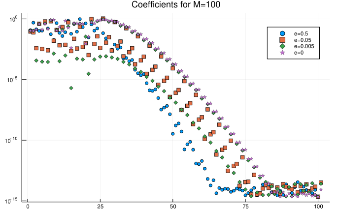
Refer to caption
Figure 3. The calculated coefficients of the interpolating polynomial on the hyperbola for 100100100 interpolation points and ϵ=0.5,0.05,0.005,0italic-ϵ0.50.050.0050\epsilon=0.5,0.05,0.005,0. The number of interpolation points is chosen sufficiently large that the interpolation coefficients approximate the true coefficients to roughly machine accuracy.

In Figure 3 we plot the coefficients of the interpolating polynomial for decreasing values of ϵitalic-ϵ\epsilon. We include ϵ=0italic-ϵ0\epsilon=0: this may appear to be a degenerate limit as L𝐿L\rightarrow\infty, but under an affine change of variables we see that the weights tend to the intersecting lines case with w(t)=1𝑤𝑡1w(t)=1 for 0t10𝑡10\leq t\leq 1 in a continuous fashion, hence we can employ the construction in Corollary 8.14. We observe super-exponential convergence for each value of ϵitalic-ϵ\epsilon, with a rate uniformly bounded as ϵ0italic-ϵ0\epsilon\rightarrow 0. This compares favourably with polynomial interpolation at Chebyshev points, which degenerates to slow algebraic convergence as ϵ0italic-ϵ0\epsilon\rightarrow 0.

Refer to caption
Refer to caption
Figure 4. The condition number of the interpolation (Vandermonde) matrix associated to a naïve basis consisting of {Tj(t)}j=0n1superscriptsubscriptsubscript𝑇𝑗𝑡𝑗0𝑛1\{T_{j}(t)\}_{j=0}^{n-1} and {t2+ϵ2Tj(t)}j=0n1superscriptsubscriptsuperscript𝑡2superscriptitalic-ϵ2subscript𝑇𝑗𝑡𝑗0𝑛1\{\sqrt{t^{2}+\epsilon^{2}}T_{j}(t)\}_{j=0}^{n-1} at 2n2𝑛2n Chebyshev points (left, log-scale) compared to the interpolation (Vandermonde) matrix using OPs on the hyperbola at the associated 2n2𝑛2n interpolation points (right, standar-scale) for ϵ=0.5,0.05,0.005,0italic-ϵ0.50.050.0050\epsilon=0.5,0.05,0.005,0. The proposed scheme has only linear growth in condition number, compared to exponential growth for the naïve basis.

Note that there is an alternative approach of approximating the solution using standard bases, for example, we could naïvely write

f(t)k=0n1fk1Tk(t)+t2+ϵ2k=0n1fk2Tk(t).𝑓𝑡superscriptsubscript𝑘0𝑛1superscriptsubscript𝑓𝑘1subscript𝑇𝑘𝑡superscript𝑡2superscriptitalic-ϵ2superscriptsubscript𝑘0𝑛1superscriptsubscript𝑓𝑘2subscript𝑇𝑘𝑡f(t)\approx\sum_{k=0}^{n-1}f_{k}^{1}T_{k}(t)+\sqrt{t^{2}+\epsilon^{2}}\sum_{k=0}^{n-1}f_{k}^{2}T_{k}(t).

The benefit of the proposed construction in terms of orthogonal polynomials on the hyperbola is that the orthogonality ensures that the interpolation is well-conditioned, whereas the standard approach results in exponentially bad conditioning, see Figure 4. Recent advances in approximation with frames can overcome the issues with ill-conditioning for the approximation problem (see [7] and references), but at the expense of no longer interpolating the data. It remains open how to use these techniques for the solution of differential equations as in Example 3.

9.2.2. Example 2: essential singularity

We now consider a function that is smooth in t𝑡t and 1/t1𝑡1/t, for example,

f(t)=sin(t+2/t)𝑓𝑡𝑡2𝑡f(t)=\sin(t+2/t)

on the real line. We project f𝑓f to the two-branch hyperbola x2=y2+1superscript𝑥2superscript𝑦21x^{2}=y^{2}+1 by the change of variables t=xy𝑡𝑥𝑦t=x-y:

f(x,y)=f(xy)=sin(xy+2(x+y))𝑓𝑥𝑦𝑓𝑥𝑦𝑥𝑦2𝑥𝑦f(x,y)=f(x-y)=\sin\left(x-y+2(x+y)\right)

where we use the fact that if t=xy𝑡𝑥𝑦t=x-y then t1=x+ysuperscript𝑡1𝑥𝑦t^{-1}=x+y since tt1=(xy)(x+y)=x2y2=1𝑡superscript𝑡1𝑥𝑦𝑥𝑦superscript𝑥2superscript𝑦21tt^{-1}=(x-y)(x+y)=x^{2}-y^{2}=1.

We repeat the procedure used in the previous example, this time with the Hermite weight:

  1. (1)

    Construct Yn,1(x,y)subscript𝑌𝑛1𝑥𝑦Y_{n,1}(x,y) using Hermite polynomials, orthogonal with respect to w(t)=et2𝑤𝑡superscript𝑒superscript𝑡2w(t)=e^{-t^{2}}.

  2. (2)

    Construct Yn,2(x,y)subscript𝑌𝑛2𝑥𝑦Y_{n,2}(x,y) using polynomials orthogonal with respect to w(t)=(1+t2)et2𝑤𝑡1superscript𝑡2superscript𝑒superscript𝑡2w(t)=(1+t^{2})e^{-t^{2}}. This construction is performed numerically using the Stieltjes procedure, with Gauss–Hermite quadrature to discretize the inner product.

  3. (3)

    Calculate the coefficients of the interpolation polynomial fM(x,y)subscript𝑓𝑀𝑥𝑦f_{M}(x,y), which equals f(x,y)𝑓𝑥𝑦f(x,y) at the M=2ν𝑀2𝜈M=2\nu points {(±xj,yj)}j=1νsuperscriptsubscriptplus-or-minussubscript𝑥𝑗subscript𝑦𝑗𝑗1𝜈\{(\pm x_{j},y_{j})\}_{j=1}^{\nu}, where yjsubscript𝑦𝑗y_{j} are the ν𝜈\nu Gauss–Hermite quadrature points and xj=yj2+1subscript𝑥𝑗superscriptsubscript𝑦𝑗21x_{j}=\sqrt{y_{j}^{2}+1}, via Corollary 8.12.

  4. (4)

    The function

    fM(t)=f(t+t12,tt12)subscript𝑓𝑀𝑡𝑓𝑡superscript𝑡12𝑡superscript𝑡12f_{M}(t)=f\left({t+t^{-1}\over 2},{t-t^{-1}\over 2}\right)

    interpolates f(t)𝑓𝑡f(t) at the M𝑀M points {±xjyj}j=1νsuperscriptsubscriptplus-or-minussubscript𝑥𝑗subscript𝑦𝑗𝑗1𝜈\{\pm x_{j}-y_{j}\}_{j=1}^{\nu}.

Refer to caption
Refer to caption
Figure 5. The coefficients of the 200 point interpolant of sin(x+2/x)𝑥2𝑥\sin(x+2/x) (top), using high precision arithmetic. Convergence of the interpolants as M𝑀M increases (bottom).

In Figure 5, we plot the decay in the coefficients of the interpolating polynomial of sin(t+2/t)𝑡2𝑡\sin(t+2/t) calculated via the proposed quadrature rule, showing an exponential decay rate. We also plot the pointwise convergence of the interpolant, showing exponentially fast uniform convergence in compact sets bounded away from the singularity t=0𝑡0t=0. Note the convergence is uniform everywhere (including at the singularity) in a weighted sense.

9.3. Solving differential equations with singular variable coefficients

As a final example, we consider the solution of Schrödinger’s equation with a nearly singular well:

h2u′′(t)+V(t)u=λusuperscript2superscript𝑢′′𝑡𝑉𝑡𝑢𝜆𝑢-h^{2}u^{\prime\prime}(t)+V(t)u=\lambda u

where we take h=0.10.1h=0.1 and V(t)=t2+ϵ2+(t0.1)2𝑉𝑡superscript𝑡2superscriptitalic-ϵ2superscript𝑡0.12V(t)=\sqrt{t^{2}+\epsilon^{2}}+(t-0.1)^{2}, and use Dirichlet conditions on the interval 3t33𝑡3-3\leq t\leq 3. As ϵ0italic-ϵ0\epsilon\rightarrow 0 the potential becomes increasingly degenerate until it is non-differentiable and approaches |t|+(t0.1)2𝑡superscript𝑡0.12|t|+(t-0.1)^{2}. For large ϵitalic-ϵ\epsilon and ϵ=0italic-ϵ0\epsilon=0 standard spectral method techniques are applicable using Chebyshev or piecewise Chebyshev approximations as implemented in Chebfun (via quantumstates command) [1] or ApproxFun.jl [8]. However, the computations quickly become infeasible as ϵitalic-ϵ\epsilon becomes small but non-zero: for example, with ϵ=0.1italic-ϵ0.1\epsilon=0.1 we require roughly 1000 coefficients (hence the solution of a 1000×1000100010001000\times 1000 eigenvalue problem) to calculate the smallest eigenvalue, while with ϵ=0.01italic-ϵ0.01\epsilon=0.01 we were unable to succeed even using 500050005000 coefficients.

As an alternative, we will use OPs on a hyperbola via the change of variables t=y𝑡𝑦t=y and x=t2+ϵ2𝑥superscript𝑡2superscriptitalic-ϵ2x=\sqrt{t^{2}+\epsilon^{2}} so that the potential is well-resolved by our basis. We then discretise the differential equation using a collocation system using 2n22𝑛22n-2 points as in the interpolation scheme above, where 2n2𝑛2n is the total number of coefficients. For simplicity of implementation, the second derivatives of the basis are calculated using automatic-differentiation (via TaylorSeries.jl [2]), however, we could also achieve this analytically by differentiating the three-term recurrence: that is, if we have the recurrence coefficients of the univariate orthogonal polynomials we can differentiate the relationship

(Jx)(p0(x)p1(x))=0𝐽𝑥matrixsubscript𝑝0𝑥subscript𝑝1𝑥0(J-x)\begin{pmatrix}p_{0}(x)\\ p_{1}(x)\\ \vdots\end{pmatrix}=0

to find a recurrence relationship for the derivative,

(Jx)(p0(x)p1(x))=(p0(x)p1(x)),𝐽𝑥matrixsuperscriptsubscript𝑝0𝑥superscriptsubscript𝑝1𝑥matrixsubscript𝑝0𝑥subscript𝑝1𝑥(J-x)\begin{pmatrix}p_{0}^{\prime}(x)\\ p_{1}^{\prime}(x)\\ \vdots\end{pmatrix}=\begin{pmatrix}p_{0}(x)\\ p_{1}(x)\\ \vdots\end{pmatrix},

and thereby determine pn(x)superscriptsubscript𝑝𝑛𝑥p_{n}^{\prime}(x) by forward substitution. Finally, we impose Dirichlet conditions as two extra rows, leading to a generalised finite-dimensional eigenvalue problem. For ϵ=0.1italic-ϵ0.1\epsilon=0.1 we confirm the calculation matches that of a standard Chebyshev spectral method (to at least 10 digits).
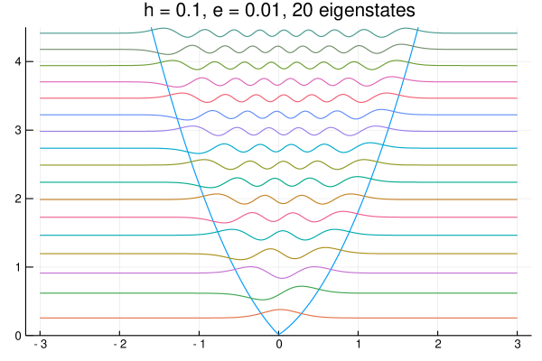
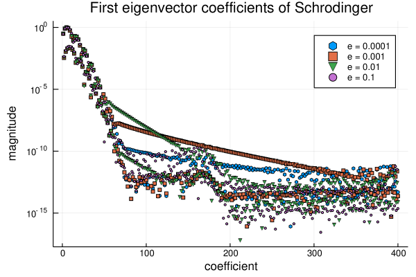
Refer to caption
Figure 6. The first 20 eigenstates for Schrödinger equation with nearly singular potential V(t)=t2+ϵ2+(t0.1)2𝑉𝑡superscript𝑡2superscriptitalic-ϵ2superscript𝑡0.12V(t)=\sqrt{t^{2}+\epsilon^{2}}+(t-0.1)^{2} with ϵ=0.01italic-ϵ0.01\epsilon=0.01. The eigenstates are shifted by the corresponding eigenvalue and scaled to fit inside the figure.
Refer to caption
Figure 7. The coefficients of the smallest energy eigenstate in OPs on the hyperbola for Schrödinger equation with nearly singular potential V(t)=t2+ϵ2+(t0.1)2𝑉𝑡superscript𝑡2superscriptitalic-ϵ2superscript𝑡0.12V(t)=\sqrt{t^{2}+\epsilon^{2}}+(t-0.1)^{2} for ϵ=0.1,0.01,0.001,0.0001italic-ϵ0.10.010.0010.0001\epsilon=0.1,0.01,0.001,0.0001, using a 400×400400400400\times 400 collocation system.

In Figure 6 we plot the first 20 eigenstates with ϵ=0.01italic-ϵ0.01\epsilon=0.01. In Figure 7 we depict the calculated coefficients of the smallest energy eigenstate in OPs on the hyperbola. We can see that the first eigenstate continues to be resolved even for ϵ=0.0001italic-ϵ0.0001\epsilon=0.0001, though there is some plateaux effect as ϵ0italic-ϵ0\epsilon\rightarrow 0. While the decay rate of the plateaux degenerates, the maginitude of the plateaux improves with smaller ϵitalic-ϵ\epsilon hence we continue to achieve high accuracy computations.

10. Future work

We have explored orthogonal polynomials on quadratic curves, and shown for weights satisfying certain symmetry properties that they can be constructed explicitly using orthogonal polynomials in one variable. We have used these orthogonal polynomials as a basis to interpolate functions with singularities of the form |x|𝑥|x|, x2+ϵ2superscript𝑥2superscriptitalic-ϵ2\sqrt{x^{2}+\epsilon^{2}}, and 1/x1𝑥1/x, where the coefficients of the interpolant are determined via quadrature rules. Exponential or super-exponential convergence was observed in each case. We showed that the construction is also applicable to solving differential equations with nearly singular variable coefficients.

Further applications of this work are to function approximation, quadrature rules, and solving differential equations involving other quadratic singularities, for example, functions that are smooth in x𝑥x and x𝑥\sqrt{x} on [0,1]01[0,1]. Such functions arise naturally in numerical methods for half-order Riemann–Liouville and Caputo fractional differential equations [5]. Orthogonal polynomials on a half-parabola—that is y2=xsuperscript𝑦2𝑥y^{2}=x, 0<x<10𝑥10<x<1—would form a natural and convenient basis for approximating such functions. However, we are left with the task of constructing orthogonal polynomials for a weight that does not satisfy the requisite symmetry properties that allowed for reduction to univariate orthogonal polynomials.

Orthogonal polynomials on quadratic curves are also of use in partial differential equations on exotic geometries, for example, they have been recently used by Snowball and the first author for solving partial differential equations on disk slices and trapeziums [12]. Finally, we mention that the results can be extended to higher dimensions, in particular to quadratic surfaces of revolution [10]. It is also likely possible to reduce orthogonal polynomials on higher dimensional geometries satisfying suitable symmetry relationships to one-dimensional orthogonal polynomials, as is the case for multivariate orthogonal polynomials with weights that are invariant under symmetry reductions [3].

A natural question that arises is the structure of orthogonal polynomials on general (higher than quadratic) algebraic curves and surfaces. A closely related question is the structure of orthogonal polynomials inside algebraic curves and surfaces. It is unlikely that we will be able to reduce orthogonal polynomials on general algebraic geometries to one variable orthogonal polynomials, so other techniques will be necessary. Understanding this structure could lead to further applications in function approximation and numerical methods for partial differential equations, as well as theoretical results.


Acknowledgment. We thank the referee for her/his carful reading and constructive comments.

References

  • [1] T. A. Driscoll, N. Hale, and L. N. Trefethen, Chebfun guide, 2014t.
  • [2] L. Benet, D. P. Sanders, and others, TaylorSeries.jl v0.10, https://github.com/JuliaDiff/TaylorSeries.jl
  • [3] C. F. Dunkl and Y. Xu, Orthogonal Polynomials of Several Variables, 2nd ed. Encyclopedia of Mathematics and its Applications 155, Cambridge University Press, 2014.
  • [4] W. Gautschi, Orthogonal Polynomials: Computation and Approximation, Oxford University Press, 2004.
  • [5] N. Hale and S. Olver, A fast and spectrally convergent algorithm for rational-order fractional integral and differential equations, SIAM J. Sci. Comp., 40 (2018) A2456–A2491.
  • [6] D. Huybrechs, On the Fourier extension of non-periodic functions, SIAM J. Numer. Anal., 47 (2010), 4326–4355.
  • [7] R. Matthysen and D. Huybrechs, Fast algorithms for the computation of Fourier extensions of arbitrary length, SIAM J. Sci. Comp., 38 (2016), A899–A922.
  • [8] S. Olver and others, ApproxFun.jl v0.11.7, https://github.com/JuliaApproximation/ApproxFun.jl
  • [9] S. Olver and Y. Xu, Orthogonal structure on a wedge and on the boundary of a square, Found. Comput. Maths, 19 (2019), 561–589.
  • [10] S. Olver and Y. Xu, Orthogonal polynomials in and on a quadratic surface of revolution, arXiv:1906.12305, 2019.
  • [11] B. Simon, Orthogonal Polynomials on the Unit Circle, American Mathematical Soc., 2005.
  • [12] B. Snowball and S. Olver, Sparse spectral and p-finite element methods for partial differential equations on disk slices and trapeziums, arXiv:1906.07962, 2019.
  • [13] G. Szegő, Orthogonal Polynomials, 4th edition, Amer. Math. Soc., Providence, RI. 1975.
  • [14] A. Zygmund, Trigonometric Series, Cambridge Univ. Press, Cambridge, 1959.