Optimal Exploitation of a Resource
with Stochastic Population Dynamics
and Delayed Renewal

Abstract

In this work, we study the optimization problem of a renewable resource in finite time. The resource is assumed to evolve according to a logistic stochastic differential equation. The manager may harvest partially the resource at any time and sell it at a stochastic market price. She may equally decide to renew part of the resource but uniquely at deterministic times. However, we realistically assume that there is a delay in the renewing order. By using the dynamic programming theory, we may obtain the PDE characterization of our value function. To complete our study, we give an algorithm to compute the value function and optimal strategy. Some numerical illustrations will be equally provided.

Key words : impulse control, renewable resource, optimal harvesting, execution delay, viscosity solutions, states constraints.

MSC Classification (2010) : 93E20, 62L15, 49L20, 49L25, 92D25

1 Introduction

The management of renewable resources is fundamental for the survival and growth of the human population. An excessive exploitation of such resources may lead to their extinction and may therefore affect the economies of depending populations with, for instance, high increases of prices and higher uncertainty on the future. The typical examples are fishery [8, 14, 17] or forest management [3, 9]. Most early studies in fishery or forest management were mainly focusing on identifying the optimal harvesting policy. In forest economics literature, it may be illustrated by the well-known “tree-cutting” problem. The most basic “tree-cutting” problem is about identifying the optimal time to harvest a given forest. Studies extending this initial tree-cutting problem have been carried by many authors. We may, for instance, refer to [9] and [20], where the authors investigate both single and ongoing rotation problems under stochastic prices and forest’s age or size. Rotation problem means once all the trees are harvested, plantation takes place and planted trees may grow up to the next harvest. In terms of mathematical formulation, rotation problem may be reduced to an iterative optimal stopping problem. In [16], the authors go a step further by studying optimal replanting strategy. To be more precise, they analyze optimal tree replanting on an area of recently harvested forest land. However, the attempt to incorporate replanting policy in the study of tree-cutting problem remains relatively very few, especially when delay has to be taken into account. Indeed, the renewed resources need some delay to become available for harvesting. There is also an uncertainty on the renewed quantities. In other words, the resource obtained after a renewing decision may differ from the expected one due to some losses. To our knowledge, these above aspects are not taken into account in the existing literature on renewable resources management. The aim of this paper is precisely to provide a more realistic model in the study of optimal exploitation problems of renewable resources by taking into account all the above features.

We suppose that the resource population evolves according to a stochastic logistic diffusion model. Such a logistic dynamics is classic in the modelling of populations evolution. The stochastic aspect allows us to take into account the uncertainties of the evolution. Since the interventions of the manager are not continuous in practice, we consider a stochastic impulse control problem on the resource population. We suppose that the operator has the ability to act on the resource population through two types of interventions. First, the manager may decide to harvest the resource and sell the harvested resource at a given exogenous market price. The second kind of intervention consists in renewing the resource. Due to physical or biological constraints, the effect of renewing orders may have some delay, i.e. a lag between the times at which renewing decisions are taken and the time at which renewed quantities appear in the global inventory of the available resources. Renewing or harvesting orders are assumed to carry both fixed and proportional costs.

From a mathematical point of view, control problems with delay have been studied in [6] and [19], where all interventions are delayed. Our model may be considered as more general since some interventions are delayed while some others are not. Another novelty of our model is the state constraints. Indeed, the level of owned resource is a physical quantity, and hence cannot be negative. Control problems under state constraints, but without delay, have been studied in the literature, see for instance [18] for the study of optimal portfolio management under liquidity constraints. To deal with such problems, the usual approach is to consider the notion of constrained viscosity solutions introduced by Soner in [23, 24]. This definition means that the value function associated to the constrained problem is a viscosity solution in the interior of the domain and only a semi-solution on the boundary. In particular, the uniqueness of the viscosity solution is usually obtained only on the interior of the domain.

In our case, we are able to characterize the behavior of the value function on the boundary by deriving the PDE satisfied on the frontier of the constrained domain. We therefore get the uniqueness property of the value function on the whole closure of the constrained domain. As a by product, we obtain the continuity of the value function on the closure of the domain (except at renewing dates), which improves the existing literature where this property is obtained only on the interior of the domain, see for instance [18].

To complete our study, we provide an algorithm to compute the value function and an associated strategy that is expected to be optimal and apply this algorithm on a specific example.

The rest of the paper is organized as follows. In Section 2, we describe the model and the associated impulse control problem. In Section 3, we give a characterization of the value function as the unique viscosity solution to a PDE in the class of functions satisfying a given growth condition. In Section 4, we provide an algorithm to compute the value function and an optimal strategy. Finally Section 5 is devoted to the proof of the main results.

2 Problem formulation

2.1 The control problem

Let $(\Omega,{\cal F},\mathbb{P})$ be a complete probability space, equipped with two mutually independent one-dimensional standard Brownian motions $B$ and $W$. We denote by $\mathbb{F}:=({\cal F}_{t})_{t\geq 0}$ the right-continuous and complete filtration generated by $B$ and $W$.

We consider a manager who owns a field of some given resource, which may be exploited up to a finite horizon time $T>0$. The aim of the manager is to manage optimally this resource in order to maximize the expected terminal wealth which may be extracted.

In resource management, the manager may decide to either harvest part of the resource or renew it. Resource renewal may be done only at discrete times $(t_{i})_{1\leq i\leq n}$ with $t_{i}=i{T\over n}$, where $n\in\mathbb{N}^{*}$. We consider an impulse control strategy $\alpha=(t_{i},\xi_{i})_{1\leq i\leq n}\cup(\tau_{k},\zeta_{k})_{k\geq 1}$ where

• $\xi_{i}$, $1\leq i\leq n$, is an ${\cal F}_{t_{i}}$-measurable random variable valued in a compact set $[0,K]$, with $K$ being a positive constant, and corresponds to the maximal quantity of resource that the manager can renew,

• $(\tau_{k})_{k\geq 1}$ a nondecreasing finite or infinite sequence of $\mathbb{F}$-stopping times representing the harvest times before $T$,

• $\zeta_{k}$, $k\geq 1$, an ${\cal F}_{\tau_{k}}$-measurable random variable, valued in $\mathbb{R}_{+}$, corresponding to the harvested quantity of resource at time $\tau_{k}$.

We assume the quantity of resource renewed at time $t_{i}$ cannot be harvested before time $t_{i}+\delta$ for any $1\leq i\leq n$ where $\delta=m{T\over n}$ with $m$ a nonnegative integer. We suppose that for a given quantity $\xi_{i}$ of resource renewed at time $t_{i}$, the manager may get an additional $g(\xi_{i})$ harvestable resource at time $t_{i}+\delta=t_{i+m}$, with $g$ being a function satisfying the following assumption.

(H$g$) $g:~{}\mathbb{R}_{+}\rightarrow\mathbb{R}_{+}$ is a nondecreasing and Lipschitz continuous function: there exists a positive constant $L$ such that

$$|g(x)-g(x^{\prime})| \leq L|x-x^{\prime}|\;,$$

for all $x,x^{\prime}\in\mathbb{R}_{+}$.

For a given strategy $\alpha=(t_{i},\xi_{i})_{1\leq i\leq n}\cup(\tau_{k},\zeta_{k})_{k\geq 1}$, we denote by $R^{\alpha}_{t}$ the associated size of resource which is available for harvesting at time $t$. When no intervention of the manager occurs, the evolution of the process $R^{\alpha}$ is assumed to follow the below logistic stochastic differential equation

$$dR^{\alpha}_{t} = \eta R^{\alpha}_{t}(\lambda-R^{\alpha}_{t})dt+\gamma R^{\alpha}_{t}dB_{t}\;,$$ (2.1)

where $\eta$, $\lambda$ and $\gamma$ are three positive constants. Since at each time $\tau_{k}$, the quantity $\zeta_{k}$ is harvested we have

$$R^{\alpha}_{\tau_{k}} = R^{\alpha}_{\tau_{k}^{-}}-\zeta_{k}\;.$$

Moreover, we suppose that there is a natural renewal of the resource at each time $t_{i}$ of a deterministic quantity $g_{0}\geq 0$. Since the renewed quantity $\xi_{i}$ at time $t_{i}$ only appears in the total resource at time $t_{i}+\delta=t_{i+m}$ and increases this one of $g(\xi_{i})$, we have

$$R^{\alpha}_{t_{i}} = R^{\alpha}_{t_{i}^{-}}+g_{0}+g(\xi_{i-m})\;,$$

for $i=m+1,\ldots,n$, and

$$R^{\alpha}_{t_{i}} = R^{\alpha}_{t_{i}^{-}}+g_{0}\;,$$

for $i=1,\ldots,m$.

The process $R^{\alpha}$ is then given by

$$R^{\alpha}_{t} = R_{0}+\int_{0}^{t}\eta R^{\alpha}_{s}(\lambda-R^{\alpha}_{s})ds+\int_{0}^{t}\gamma R^{\alpha}_{s}dB_{s}$$ (2.2)

$$-\sum_{k\geq 1}\zeta_{k}{\mathds{1}}_{\tau_{k}\leq t}+\sum_{i=1}^{n}g(\xi_{i}){\mathds{1}}_{t_{i+m}\leq t}+g_{0}\sum_{i=1}^{n}{\mathds{1}}_{t_{i}\leq t}\;,\quad t\geq 0\;.$$

We assume that the price $P$ by unit of the resource is governed by the following stochastic differential equation

$$P_{t} = P_{0}+\int_{0}^{t}\mu P_{u}du+\int_{0}^{t}\sigma P_{u}dW_{u}\;,\quad t\geq 0\;,$$ (2.3)

with $\mu$ and $\sigma$ two positive constants.

We also define $Q_{t}$ the cost at time $t$ to renew a unit of the resource. We suppose that it follows the below stochastic differential equation

$$Q_{t} = Q_{0}+\int_{0}^{t}\rho Q_{u}du+\int_{0}^{t}\varsigma Q_{u}dW_{u}\;,\quad t\geq 0\;,$$ (2.4)

where $\rho$ and $\varsigma$ are two positive constants.

For a given strategy $\alpha=(t_{i},\xi_{i})_{1\leq i\leq n}\cup(\tau_{k},\zeta_{k})_{k\geq 1}$, there are several costs that the manager has to face.

• At each time $\tau_{k}$, the manager has to pay a cost $c_{1}\zeta_{k}+c_{2}$ to harvest the quantity $\zeta_{k}$, where $c_{1}$ and $c_{2}$ are two positive constants. As such, by selling the harvested quantity $\zeta_{k}$ at price $P_{\tau_{k}}$, she may get $(P_{\tau_{k}}-c_{1})\zeta_{k}-c_{2}$ at time $\tau_{k}$.

• To renew quantity $\xi_{i}$ of resource at time $t_{i}$, the manager has to pay $(Q_{t_{i}}+c_{3})\xi_{i}$, where $c_{3}$ is a positive constant.

Given a control $\alpha=(t_{i},\xi_{i})_{1\leq i\leq n}\cup(\tau_{k},\zeta_{k})_{k\geq 1}$ and an initial wealth $X_{0}$, the wealth process $X^{\alpha}$ may be expressed as follows

$$X_{t}^{\alpha} = X_{0}+\sum_{k\geq 1}\big{[}(P_{\tau_{k}}-c_{1})\zeta_{k}-c_{2}\big{]}{\mathds{1}}_{\tau_{k}\leq t}-\sum_{i=1}^{n}(Q_{t_{i}}+c_{3})\xi_{i}{\mathds{1}}_{t_{i}\leq t}\;.$$

We define the set ${\cal A}$ of admissible controls as the set of strategies $\alpha$ such that

$$\mathbb{E}\Big{[}(X_{T}^{\alpha})^{-}\Big{]}~{}<~{}+\infty R^{\alpha}_{t}\geq 0\quad\text{for }0\leq t\leq T\;,$$ and (2.5)

where $(.)^{-}$ denotes the negative part. We note that for $R_{0}\geq 0$, the set ${\cal A}$ is nonempty as it contains the strategy with no intervention.

We denote by ${\cal Z}$ the set ${\cal Z}:=\mathbb{R}\times\mathbb{R}_{+}\times\mathbb{R}_{+}^{*}\times\mathbb{R}_{+}^{*}$. We define the liquidation function $L:~{}{\cal Z}\rightarrow\mathbb{R}$ by

$$L(z) := \max\{x+(p-c_{1})r-c_{2},x\}\;,\quad\mbox{ for }~{}z=(x,r,p,q)\in{\cal Z}\;.$$

From condition (2.5), the expectation $\mathbb{E}[L(X_{T}^{\alpha},R_{T}^{\alpha},P_{T},Q_{T})]$ is well defined for any $\alpha\in{\cal A}$. We can therefore consider the objective of the manager which consists in computing the optimal value

$$V_{0} := \sup_{\alpha\in{\cal A}}\mathbb{E}\big{[}L(X_{T}^{\alpha},R_{T}^{\alpha},P_{T},Q_{T})\big{]}\;,$$ (2.6)

and finding a strategy $\alpha^{*}\in{\cal A}$ such that

$$V_{0} = \mathbb{E}\big{[}L(X_{T}^{\alpha^{*}},R_{T}^{\alpha^{*}},P_{T},Q_{T})\big{]}\;.$$ (2.7)

2.2 Value functions with pending orders

In order to provide an analytic characterization of the value function $V$ defined by the control problem (2.6), we need to extend the definition of this control problem to general initial conditions. Moreover, since the renewing decisions are delayed, we have to take into account the possible pending orders.

Given an impulse control $\alpha\in{\cal A}$, we notice that the state of the system $R^{\alpha}$ is not only defined by its current state value at time $t$ but also by the quantity at time $t$ of the resource that has been renewed between $t-\delta$ and $t$. We therefore introduce the following definitions and notations. For any $t\in[0,T]$, we denote by $N(t)$ the number of possible renewing dates before $t$

$$N(t) := \#\Big{\{}i\in\{1,\ldots,n\}~{}:~{}t_{i}\leq t\Big{\}}\;,$$

and by $D_{t}$ the set of renewing resource times and the associated quantities between $t-\delta$ and $t$

$$D_{t} := \Big{\{}d=(t_{i},e_{i})_{N(t-\delta)+1\leq i\leq N(t)}~{}:~{}e_{i}\in\mathbb{R}_{+}\mbox{ for }i=N(t-\delta)+1,\ldots,N(t)\Big{\}}\;,\quad$$ (2.8)

with the convention that $D_{t}=\emptyset$ if $N(t-\delta)=N(t)$.

For any $t\in[0,T]$ and $d=(t_{i},e_{i})_{N(t-\delta)+1\leq i\leq N(t)}\in D_{t}$, we denote by $\tilde{\cal A}_{t,d}$ the set of strategies which take into account the pending renewing decisions taken between $t-\delta$ and $t$

$$\tilde{\cal A}_{t,d} := \Big{\{}\alpha=(t_{i},\xi_{i})_{N(t-\delta)+1\leq i\leq n}\cup(\tau_{k},\zeta_{k})_{k\geq 1}~{}:~{}$$

$$\quad\xi_{i}=e_{i}~{}\mbox{ for }~{}i=N(t-\delta)+1,\ldots,N(t)\;;$$

$$\quad\xi_{i}\mbox{ is }{\cal F}_{t_{i}}-\mbox{measurable for }~{}N(t)+1\leq i\leq n\;;$$

$$\quad(\tau_{k})_{k\geq 1}\mbox{ is a nondecreasing finite or infinite sequence of }\mathbb{F}-\mbox{stopping time}\mbox{ with }\tau_{1}>t\;;$$

$$\quad\zeta_{k}\mbox{ is }{\cal F}_{\tau_{k}}-\mbox{measurable for }~{}k\geq 1\Big{\}}\;.$$

For $z=(x,r,p,q)\in{\cal Z}$, $d\in D_{t}$ and $\alpha\in\tilde{\cal A}_{t,d}$, we denote by $Z^{t,z,\alpha}=(X^{t,z,\alpha},R^{t,r,\alpha},P^{t,p},Q^{t,q})$ the quadruple of processes defined by

$$R^{t,r,\alpha}_{s} = r+\int_{t}^{s}\eta R^{t,r,\alpha}_{u}(\lambda-R^{t,r,\alpha}_{u})du+\int_{t}^{s}\gamma R^{t,r,\alpha}_{u}dB_{u}-\sum_{k\geq 1}\zeta_{k}{\mathds{1}}_{\tau_{k}\leq s}$$ (2.9)

$$+\sum_{i=N(t-\delta)+1}^{n}g(\xi_{i}){\mathds{1}}_{t_{i+m}\leq s}+g_{0}\big{(}N(s)-N(t)\big{)}\;,$$

$$X^{t,z,\alpha}_{s} = x+\sum_{k\geq 1}\big{[}(P^{t,p}_{\tau_{k}}-c_{1})\zeta_{k}-c_{2}\big{]}{\mathds{1}}_{\tau_{k}\leq s}-\sum_{i=N(t)+1}^{n}(Q^{t,q}_{t_{i}}+c_{3})\xi_{i}{\mathds{1}}_{t_{i}\leq s}\;,$$ (2.10)

$$P^{t,p}_{s} = p+\int_{t}^{s}\mu P^{t,p}_{u}du+\int_{t}^{s}\sigma P^{t,p}_{u}dW_{u}\;,$$ (2.11)

$$Q^{t,q}_{s} = q+\int_{t}^{s}\rho Q^{t,q}_{u}du+\int_{t}^{s}\varsigma Q^{t,q}_{u}dW_{u}\;,$$ (2.12)

for $s\in[t,T]$. We denote by ${\cal A}_{t,z,d}$ the set of strategies $\alpha\in\tilde{\cal A}_{t,d}$ such that

$$\mathbb{E}\Big{[}(X^{t,z,\alpha}_{T})^{-}\Big{]}~{}<~{}+\infty R^{t,r,\alpha}_{s}\geq 0\quad\text{for all }s\in[t,T]\;.\qquad$$ and (2.13)

We then consider for $(t,z)\in[0,T]\times{\cal Z}$, $d\in D_{t}$, $\alpha\in{\cal A}_{t,z,d}$ the following benefit criterion

$$J(t,z,\alpha) := \mathbb{E}\Big{[}L(Z^{t,z,\alpha}_{T})\Big{]}\;,$$

which is well defined under conditions (2.13). We define the corresponding value function by

$$v(t,z,d) := \sup_{\alpha\in{\cal A}_{t,z,d}}J(t,z,\alpha)\;,\quad(t,z,d)\in\mathcal{D}\;,$$

where $\mathcal{D}$ is the definition domain of $v$ defined by

$${\cal D} = \Big{\{}(t,z,d)~{}:~{}(t,z)\in[0,T]\times{\cal Z}\mbox{ and }d\in D_{t}\Big{\}}\;.$$

For simplicity, we also introduce the operators $\Gamma^{c}$, $\Gamma^{rn}_{1}$ and $\Gamma^{rn}_{2}$ given by

$$\Gamma^{c}(z,\ell) := (x+(p-c_{1})\ell-c_{2},r-\ell,p,q)\;,$$

$$\Gamma^{rn}_{1}(z,\ell) := (x-(q+c_{3})\ell,r+g_{0},p,q)\;,$$

$$\Gamma^{rn}_{2}(z,\ell) := (x,r+g(\ell),p,q)\;,$$

for all $z=(x,r,p,q)\in{\cal Z}$ and $\ell\in\mathbb{R}_{+}$. The operator $\Gamma^{c}$ corresponds to the new position of the state process after a resource consumption decision: if the manager harvests $\zeta_{k}$ at time $\tau_{k}$, then the state process is

$$Z^{t,z,\alpha}_{\tau_{k}} = \Gamma^{c}(Z^{t,z,\alpha}_{\tau_{k}^{-}},\zeta_{k})\;,$$

and $\Gamma^{rn}_{1}$ and $\Gamma^{rn}_{2}$ correspond to the new position of the state process after a renewal decision: if the manager renews $(\xi_{i})_{1\leq i\leq n}$ at times $(t_{i})_{1\leq i\leq n}$, then the state process is given by

$$Z^{t,z,\alpha}_{t_{i}} = \Gamma^{rn}_{1}(Z^{t,z,\alpha}_{t_{i}^{-}},\xi_{i})\;,\quad\mbox{for }i=0,\ldots,m\;,$$

$$Z^{t,z,\alpha}_{t_{i}} = \Gamma^{rn}_{1}(\Gamma^{rn}_{2}(Z^{t,z,\alpha}_{t_{i}^{-}},\xi_{i-m}),\xi_{i})\;,\quad\mbox{for }i=m+1,\ldots,n\;.$$

We first give a new expression of the value function $v$. To this end, we introduce the set

$$\hat{\cal A}_{t,z,d} = \Big{\{}\alpha=(t_{i},\xi_{i})_{N(t-\delta)+1\leq i\leq n}\cup(\tau_{k},\zeta_{k})_{k\geq 1}\in\tilde{\cal A}_{t,d}~{}:$$

$$~{}\big{(}P^{t,p}_{\tau_{k}}-c_{1}\big{)}\zeta_{k}-c_{2}~{}\geq~{}0~{}\forall\,k\geq 1~{}\mbox{ and }R^{t,r,\alpha}_{s}\geq 0~{}\forall\,s\in[t,T]\Big{\}}\;.$$

Proposition 2.1.

The value function $v$ can be expressed as follows

$$v(t,z,d) = \sup_{\alpha\in\hat{\cal A}_{t,z,d}}J(t,z,\alpha)\;,\quad(t,z,d)\in\mathcal{D}\;.$$ (2.14)

Proof. Fix $(t,z,d)\in\mathcal{D}$ with $z=(x,r,p,q)$ and denote by $\hat{v}(t,z,d)$ the right hand side of (2.14).

We first notice that $\hat{\cal A}_{t,z,d}\subset{\cal A}_{t,z,d}$. Indeed, for $\alpha\in\hat{\cal A}_{t,z,d}$, we have

$$X^{t,z,\alpha}_{T} = x+\sum_{k\geq 1}\big{[}(P^{t,p}_{\tau_{k}}-c_{1})\zeta_{k}-c_{2}\big{]}{\mathds{1}}_{\tau_{k}\leq T}-\sum_{i=N(t)+1}^{n}(Q^{t,q}_{t_{i}}+c_{3})\xi_{i}$$

$$\geq x-nK\big{(}\sup_{s\in[t,T]}Q^{t,q}_{s}+c_{3}\big{)}\;.$$

Since $Q^{t,q}$ follows the dynamics (2.12), we have $\mathbb{E}[\sup_{s\in[t,T]}Q^{t,q}_{s}]<+\infty$ and we get $\mathbb{E}[(X^{t,z,\alpha}_{T})^{-}]<+\infty$. We therefore deduce that

$$v(t,z,d) \geq \hat{v}(t,z,d)\;.$$

We turn to the reverse inequality. Fix $\alpha=(t_{i},\xi_{i})_{N(t-\delta)+1\leq i\leq n}\cup(\tau_{k},\zeta_{k})_{k\geq 1}\in{\cal A}_{t,z,d}$ and define the associated strategy $\hat{\alpha}=(t_{i},\xi_{i})_{N(t-\delta)+1\leq i\leq n}\cup(\hat{\tau}_{k},\hat{\zeta}_{k})_{k\geq 1}\in\hat{\cal A}_{t,z,d}$ by

$$(\hat{\tau}_{j},\hat{\zeta}_{j}) = (\tau_{k_{j}},\zeta_{k_{j}})\quad~{}~{}\mbox{ for }j\geq 1\;,$$

where the sequence $(k_{j})_{j\geq 1}$ is defined by

$$k_{1} = \min\{k\geq 1~{}:~{}(P^{t,p}_{\tau_{k}}-c_{1})\zeta_{k}-c_{2}\geq 0\}\;,$$

$$k_{j} = \min\{k\geq k_{j-1}+1~{}:~{}(P^{t,p}_{\tau_{k}}-c_{1})\zeta_{k}-c_{2}\geq 0\}\;,$$

$i.e.$ $\hat{\alpha}$ is obtained from $\alpha$ by keeping only harvesting orders such that $(P^{t,p}_{\tau_{k}}-c_{1})\zeta_{k}-c_{2}\geq 0$.

We then easily check from dynamics (2.9) and (2.10) that

$$X_{s}^{t,z,\alpha}~{}\leq~{}X_{s}^{t,z,\hat{\alpha}} R_{s}^{t,r,\alpha}~{}\leq~{}R_{s}^{t,r,\hat{\alpha}}$$ and

for all $s\in[t,T]$. Therefore we get

$$L(Z_{T}^{t,z,\alpha}) \leq L(Z_{T}^{t,z,\hat{\alpha}})\;,$$

which gives

$$\hat{v}(t,z,d) \geq v(t,z,d)\;.$$

$\Box$

3 PDE characterization

3.1 Boundary condition and dynamic programming principle

We first provide a boundary condition for the value function associated to the optimal management of renewable resource.

Proposition 3.2.

The value function $v$ satisfies the following growth condition: there exists a constant $C$ such that

$$x~{}~{}\leq~{}~{}v(t,z,d) \leq x+C\Big{(}1+|r|^{4}+|p|^{4}+|q|^{4}\Big{)}\;,\qquad$$ (3.15)

for all $t\in[0,T]$, $z=(x,r,p,q)\in{\cal Z}$, and $d\in D_{t}$.

The proof of this proposition is postponed to Section 5.1.

With this bound, we are able to state the dynamic programming relation on the value function of our control problem with execution delay. For any $t\in[0,T]$, $d\in D_{t}$ and $\alpha=(t_{i},\xi_{i})_{N(t-\delta)+1\leq i\leq n}\cup(\tau_{k},\zeta_{k})_{k\geq 1}\in\hat{\cal A}_{t,z,d}$, we denote

$$d(u,\alpha) = (t_{i},\xi_{i})_{N(u-\delta)+1\leq i\leq N(u)}\;,\quad u\in[t,T]\;,$$

with the convention that $d(u,\alpha)=\emptyset$ if $N(u-\delta)=N(u)$. We notice that $d(u,\alpha)$ corresponds to the set of renewing orders that have been given before $u$ and whose delayed effects appear after $u$. We also denote by ${\cal T}_{[t,T]}$ the set of $\mathbb{F}$-stopping times valued in $[t,T]$.

Theorem 3.1.

The value function $v$ satisfies the following dynamic programming principle.

1. First dynamic programming inequality:

   $$v(t,z,d) \geq \mathbb{E}\Big{[}v(\vartheta,Z^{t,z,\alpha}_{\vartheta},d(\vartheta,\alpha))\Big{]}\;,$$

   for all $\alpha\in\hat{\cal A}_{t,z,d}$ and all $\vartheta\in{\cal T}_{[t,T]}$.

2. Second dynamic programming inequality: for any $\varepsilon>0$, there exists $\alpha\in\hat{\cal A}_{t,z,d}$ such that

   $$v(t,z,d)-\varepsilon \leq \mathbb{E}\Big{[}v(\vartheta,Z_{\vartheta}^{t,z,\alpha},d(\vartheta,\alpha))\Big{]}\;,$$

   for all $\vartheta\in{\cal T}_{[t,T]}$.

The proof of this proposition is postponed to Section 5.2.

3.2 Viscosity properties and uniqueness

The PDE system associated to our control problem is formally derived from the dynamic programming relations. We first decompose the domain ${\cal D}$ as follows

$${\cal D} = \bigcup_{k=0}^{n}{\cal D}_{k}\;,$$

where

$${\cal D}_{k} = \Big{\{}(t,z,d)\in{\cal D}~{}:~{}~{}t\in\big{[}t_{k},t_{k+1}\big{)}\Big{\}}\;,$$

for $k=0,\ldots,n-1$ and

$${\cal D}_{n} = \Big{\{}(t,z,d)\in{\cal D}~{}:~{}t=T\Big{\}}\;.$$

We also decompose the sets ${\cal D}_{k}$, $k=0,\ldots,n$, as follows

$${\cal D}_{k} = {\cal D}_{k}^{1}\cup{\cal D}_{k}^{2}\;,$$

where

$${\cal D}_{k}^{1} = \big{\{}(t,z,d)\in{\cal D}_{k}~{}:~{}z=(x,r,p,q)\mbox{ with }r=0\big{\}}\;,$$

$${\cal D}_{k}^{2} = \big{\{}(t,z,d)\in{\cal D}_{k}~{}:~{}z=(x,r,p,q)\mbox{ with }r>0\big{\}}\;.$$

We define the operators ${\cal H}$, ${\cal N}_{1}$, $\bar{\cal N}_{1}$, ${\cal N}_{2}$ and $\bar{\cal N}_{2}$ by

$${\cal H}\phi(t,z,d) = \sup_{0\leq a\leq r}\phi\big{(}t,\Gamma^{c}(z,a),d\big{)}\;,$$

for any $(t,z,d)\in{\cal D}$ and any function $\phi$ defined on ${\cal D}$,

$${\cal N}_{1}\phi(t_{k},z,d) = \sup_{0\leq e\leq K}\phi\Big{(}t_{k},\Gamma^{rn}_{1}\big{(}\Gamma^{rn}_{2}(z,e_{k-m}),e\big{)},d\cup(t_{k},e)\setminus(t_{k-m},e_{k-m})\Big{)}\;,$$

$$\bar{\cal N}_{1}\phi(t_{k},z,d) = \sup_{\tiny\begin{array}[]{c}0\leq e\leq K\\ 0\leq a\leq r\end{array}}\phi\Big{(}t_{k},\Gamma^{rn}_{1}\big{(}\Gamma^{rn}_{2}\big{(}\Gamma^{c}(z,a),e_{k-m}\big{)},e\big{)},d\cup(t_{k},e)\setminus(t_{k-m},e_{k-m})\Big{)}\;,$$

for any $(t_{k},z,d)\in{\cal D}$ with $k=m+1,\ldots,n$, and any function $\phi$ defined on ${\cal D}$, and

$${\cal N}_{2}\phi(t_{k},z,d) = \sup_{0\leq e\leq K}\phi\Big{(}t_{k},\Gamma^{rn}_{1}\big{(}z,e\big{)},d\cup(t_{k},e)\Big{)}\;,$$

$$\bar{\cal N}_{2}\phi(t_{k},z,d) = \sup_{\tiny\begin{array}[]{c}0\leq e\leq K\\ 0\leq a\leq r\end{array}}\phi\Big{(}t_{k},\Gamma^{rn}_{1}\big{(}\Gamma^{c}(z,a),e\big{)},d\cup(t_{k},e)\Big{)}\;,$$

for any $(t_{k},z,d)\in{\cal D}$ with $k=0,\ldots,m$, and any function $\phi$ defined on ${\cal D}$.

This provides equations for the value function $v$ which takes the following nonstandard form

$$-{\cal L}v(t,z,d) = 0$$ (3.18)

for $(t,z,d)\in{\cal D}^{1}_{k}$, with $k=0,\ldots,n$,

$$\min\Big{\{}-{\cal L}v(t,z,d)~{},~{}v(t,z,d)-{\cal H}v(t,z,d)\Big{\}} = 0$$ (3.19)

for $(t,z,d)\in{\cal D}^{2}_{k}$, with $k=0,\ldots,n-1$,

$$v(T^{-},z,d) = \max\big{\{}{\cal N}_{1}L(z,d)~{},~{}\bar{\cal N}_{1}L(z,d)\big{\}}\qquad$$ (3.20)

for $(T,z,d)\in{\cal D}$,

$$v(t_{k}^{-},z,d) = \max\{{\cal N}_{1}v(t_{k},z,d)~{},~{}\bar{\cal N}_{1}v(t_{k},z,d)\}$$ (3.21)

for $(t_{k},z,d)\in{\cal D}_{k}$, with $k=m+1,\ldots,n-1$, and

$$v(t_{k}^{-},z,d) = \max\big{\{}{\cal N}_{2}v(t_{k},z,d)~{},~{}\bar{\cal N}_{2}v(t_{k},z,d)\big{\}}\qquad$$ (3.22)

for $(t_{k},z,d)\in{\cal D}_{k}$, with $k=0,\ldots,m$.

Here ${\cal L}$ is the second order local operator associated to the diffusion $(P,Q,R)$ with no intervention. It is given by

$${\cal L}\varphi(t,z) = \partial_{t}\varphi(t,z)+\mu p\partial_{p}\varphi(t,z)+\rho q\partial_{q}\varphi(t,z)+\eta r(\lambda-r)\partial_{r}\varphi(t,z)$$

$$+{1\over 2}\Big{(}\sigma^{2}p^{2}\partial^{2}_{pp}\varphi(t,z)+\varsigma^{2}q^{2}\partial^{2}_{qq}\varphi(t,z)+2\sigma\varsigma pq\partial^{2}_{pq}\varphi(t,z)+\gamma^{2}r^{2}\partial^{2}_{rr}\varphi(t,z)\Big{)}$$

for any $(t,z)\in[0,T]\times{\cal Z}$ with $z=(x,r,p,q)$ and any function $\varphi\in C^{1,2}([0,T]\times{\cal Z})$.

As usual, we do not have any regularity property on the value function $v$. We therefore work with the notion of (discontinuous) viscosity solution. Since our system of PDEs (3.18) to (3.22) is nonstandard, we have to adapt the definition to our framework.

First, for a locally bounded function $w$ defined on ${\cal D}$, we define its lower semicontinuous (resp. upper semicontinuous) envelop $w_{*}$ (resp. $w^{*}$) by

$$w_{*}(t,z,d) = \liminf_{\tiny\begin{array}[]{c}(t^{\prime},z^{\prime},d^{\prime})\rightarrow(t,z,d)\\ (t^{\prime},z^{\prime},d^{\prime})\in{\cal D}_{k}\end{array}}w(t^{\prime},z^{\prime},d^{\prime})\;,$$

$$w^{*}(t,z,d) = \limsup_{\tiny\begin{array}[]{c}(t^{\prime},z^{\prime},d^{\prime})\rightarrow(t,z,d)\\ (t^{\prime},z^{\prime},d^{\prime})\in{\cal D}_{k}\end{array}}w(t^{\prime},z^{\prime},d^{\prime})\;,$$

for $(t,z,d)\in{\cal D}_{k}$, with $k=0,\ldots,n-1$. We also define its left lower semicontinuous (resp. upper semicontinuous) envelop at time $t_{k}$ by

$$w_{*}(t_{k}^{-},z,d) = \liminf_{\tiny\begin{array}[]{c}(t^{\prime},z^{\prime},d^{\prime})\rightarrow(t_{k}^{-},z,d)\\ (t^{\prime},z^{\prime},d^{\prime})\in{\cal D}_{k-1}\end{array}}w(t^{\prime},z^{\prime},d)\;,$$

$$w^{*}(t_{k}^{-},z,d) = \limsup_{\tiny\begin{array}[]{c}(t^{\prime},z^{\prime},d^{\prime})\rightarrow(t_{k}^{-},z,d)\\ (t^{\prime},z^{\prime},d^{\prime})\in{\cal D}_{k-1}\end{array}}w(t^{\prime},z^{\prime},d)\;,$$

for $k\in\{1,\ldots,n\}$.

Definition 3.1 (Viscosity solution to (3.18) – (3.22)).

A locally bounded function $w$ defined on ${\cal D}$ is a viscosity supersolution (resp. subsolution) if

(i) for any $k=0,\ldots,n-1$, $(t,z)\in{\cal D}_{k}^{1}$ and $\varphi\in C^{1,2}({\cal D}_{k})$ such that

$$(w_{*}-\varphi)(t,z,d) = \min_{{\cal D}_{k}}(w_{*}-\varphi)$$

$$\mbox{(resp. }(w^{*}-\varphi)(t,z,d) = \max_{{\cal D}_{k}}(w^{*}-\varphi)\mbox{)}$$

we have

$$-{\cal L}\varphi(t,z,d) \geq 0$$

$$\mbox{(resp. }-{\cal L}\varphi(t,z,d) \leq 0\mbox{)}\;,$$

(ii) for any $k=0,\ldots,n-1$, $(t,z)\in{\cal D}^{2}_{k}$ and $\varphi\in C^{1,2}({\cal D}_{k})$ such that

$$(w_{*}-\varphi)(t,z,d) = \min_{{\cal D}_{k}}(w_{*}-\varphi)$$

$$\mbox{(resp. }(w^{*}-\varphi)(t,z,d) = \max_{{\cal D}_{k}}(w^{*}-\varphi)\mbox{)}$$

we have

$$\min\Big{\{}-{\cal L}\varphi(t,z,d)~{},~{}w_{*}(t,z,d)-{\cal H}w_{*}(t,z,d)\Big{\}} \geq 0$$

$$\mbox{(resp. }\min\Big{\{}-{\cal L}\varphi(t,z,d)~{},~{}w^{*}(t,z,d)-{\cal H}w^{*}(t,z,d)\Big{\}} \leq 0\mbox{)}\;,$$

(iii) for any $(T,z,d)\in{\cal D}$ we have

$$w_{*}(T^{-},z,d) \geq \max\{{\cal N}_{1}L(z,d)~{},~{}\bar{\cal N}_{1}L(z,d)\}$$

$$\mbox{(resp. }w_{*}(T^{-},z,d) \leq \max\{{\cal N}_{1}L(z,d)~{},~{}\bar{\cal N}_{1}L(z,d)\}\mbox{)}\;,$$

(iv) for any $k=m+1,\ldots,n-1$, $(t_{k},z,d)\in{\cal D}$ we have

$$w_{*}(t_{k}^{-},z,d) \geq \max\{{\cal N}_{1}w_{*}(t_{k},z,d)~{},~{}\bar{\cal N}_{1}w_{*}(t_{k},z,d)\}$$

$$\mbox{(resp. }w^{*}(t_{k}^{-},z,d) \leq \max\{{\cal N}_{1}w^{*}(t_{k},z,d)~{},~{}\bar{\cal N}_{1}w^{*}(t_{k},z,d)\}\mbox{)}\;,$$

(v) for any $k=0,\ldots,m$, $(t_{k},z,d)\in{\cal D}$ we have

$$w_{*}(t_{k}^{-},z,d) \geq \max\{{\cal N}_{2}w_{*}(t_{k},z,d)~{},~{}\bar{\cal N}_{2}w_{*}(t_{k},z,d)\}$$

$$\mbox{(resp. }w^{*}(t_{k}^{-},z,d) \leq \max\{{\cal N}_{2}w^{*}(t_{k},z,d)~{},~{}\bar{\cal N}_{2}w^{*}(t_{k},z,d)\}\mbox{)}\;.$$

A locally bounded function $w$ defined on ${\cal D}$ is said to be a viscosity solution to (3.18)–(3.22) if it is a supersolution and a subsolution to (3.18)–(3.22).

The next result provides the viscosity properties of the value function $v$.

Theorem 3.2 (Viscosity characterization).

The value function $v$ is the unique viscosity solution to (3.18)–(3.22) satisfying the growth condition (3.15). Moreover, $v$ is continuous on ${\cal D}_{k}$ for all $k=0,\ldots,n-1$.

4 Numerics

We describe, in this section, a backward algorithm to approximate the value function and an optimal strategy. Some numerical illustrations are also provided.

4.1 Approximation of the value function $v$

Initialization step.

For $(t,z,d)\in{\cal D}_{n-1}^{1}$ we have

$$v(t,z,d) = \mathbb{E}\Big{[}\max\{{\cal N}_{1}L(Z^{t,z,d}_{T},d)~{},~{}\bar{\cal N}_{1}L(Z^{t,z,d}_{T},d)\}\Big{]}\;.$$

We can therefore approximate it by $\hat{v}(t,z,d)$ which is the associated Monte Carlo estimator.

On ${\cal D}_{n-1}^{2}$ the function $v$ is solution to the PDE (3.19) with the terminal condition (3.20). Therefore, we can compute an approximation $\hat{v}$ using an algorithm computing optimal values of impulse control problem with boundary on ${\cal D}_{n-1}^{1}$ and the terminal value given by (3.20) (see e.g. [11]).

Step $k+1\rightarrow k$.

Once we have an approximation $\hat{v}(t,z,d)$ of $v(t,z,d)$ for $(t,z,d)\in{\cal D}_{k+1}$ we are able to get an approximation of $v$ on ${\cal D}_{k}$ as follows.

$\bullet$ Case 1: $m\leq k\leq n-1$.

For $(t,z,d)\in{\cal D}_{k}^{1}$ we have

$$v(t,z,d) = \mathbb{E}\Big{[}\max\{{\cal N}_{1}v(t_{k+1},Z^{t,z,d}_{t_{k+1}},d)~{},~{}\bar{\cal N}_{1}v(t_{k+1},Z^{t,z,d}_{t_{k+1}},d)\}\Big{]}\;.$$

We can therefore approximate it by $\hat{v}(t,z,d)$ which is the Monte Carlo estimator of

$$\mathbb{E}\Big{[}\max\{{\cal N}_{1}\hat{v}(t_{k+1},Z^{t,z,d}_{t_{k+1}},d)~{},~{}\bar{\cal N}_{1}\hat{v}(t_{k+1},Z^{t,z,d}_{t_{k+1}},d)\}\Big{]}\;.$$

On ${\cal D}_{k}^{2}$ the function $v$ is solution to the PDE (3.19) with the terminal condition (3.21). Since we already have approximations of $v$ on ${\cal D}^{1}_{k}$ and ${\cal D}_{k+1}$, we can compute an approximation $\hat{v}$ using an algorithm computing optimal values of impulse control problem with boundary on ${\cal D}_{k}^{1}$ (see e.g. [11]) and the terminal value given by

$$\hat{v}(t_{k+1}^{-},z,d) = \max\{{\cal N}_{1}\hat{v}(t_{k+1},z,d)~{},~{}\bar{\cal N}_{1}\hat{v}(t_{k+1},z,d)\}\;.$$

$\bullet$ Case 2: $0\leq k\leq m-1$. The procedure is the same as in Case 1 but with ${\cal N}_{2}$ and $\bar{\cal N}_{2}$ instead of ${\cal N}_{1}$ and $\bar{\cal N}_{1}$ respectively.

4.2 An optimal strategy for the approximated problem

We turn to the computation of an optimal strategy. From the general optimal stopping theory (see [13]), we provide the following strategy $\hat{\alpha}$. This strategy is constructed as usually done for optimal strategies of impulse control problem but using the approximation $\hat{v}$ instead of the value function $v$. We start with an initial data $(t,z,d)$. We denote by $\hat{\alpha}=(t_{i},\hat{\xi}_{i})_{N(t-\delta)+1\leq i\leq n}\cup(\hat{\tau}_{k},\hat{\zeta}_{k})_{k\geq 1}$ the strategy constructed step by step and by $\hat{Z}^{\kappa}=(\hat{X}^{\kappa},\hat{R}^{\kappa},\hat{P}^{\kappa},\hat{Q}^{\kappa})$ the process controlled by the truncated strategy $\hat{\alpha}^{\kappa}:=(t_{i},\hat{\xi}_{i})_{N(t-\delta)+1\leq i\leq n}\cup(\hat{\tau}_{k},\hat{\zeta}_{k})_{\kappa\geq k\geq 1}$. We also denote by $\hat{d}_{s}=(t_{i},\hat{e}_{i})_{N(s-\delta)+1\leq i\leq N(s)}$ the pending orders at time $s\in[t,T]$.

Initialization step.

We first start by computing the first harvesting time $\hat{\tau}_{1}$ by

$$\hat{\tau}_{1} = \inf\Big{\{}s\geq t~{}:~{}\hat{v}(s,\hat{Z}^{0}_{s},\hat{d}_{s})~{}=~{}{\cal H}\hat{v}(s,\hat{Z}^{0}_{s},\hat{d}_{s})\Big{\}}$$

and the associated harvested quantity $\hat{\zeta}_{1}$ by

$$\hat{\zeta}_{1} \in \text{arg}\max_{0\leq a\leq\hat{R}^{0}_{\tau_{1}}}\hat{v}(\hat{\tau}_{1},\Gamma^{c}(\hat{Z}^{0}_{\hat{\tau}_{1}},a),\hat{d}_{\hat{\tau}_{1}})\;.$$

Step $k\rightarrow k+1$ for harvesting orders.

We then compute the $(k+1)$-th harvesting time $\hat{\tau}_{k+1}$ by

$$\hat{\tau}_{k+1} = \inf\Big{\{}s\geq\hat{\tau}_{k}~{}:~{}\hat{v}(s,\hat{Z}^{k}_{s},\hat{d}_{s})~{}=~{}{\cal H}\hat{v}(s,\hat{Z}^{k}_{s},\hat{d}_{s})\Big{\}}$$

and the associated harvested quantity $\hat{\zeta}_{k+1}$ by

$$\hat{\zeta}_{k+1} \in \text{arg}\max_{0\leq a\leq\hat{R}^{k}_{\tau_{k+1}}}\hat{v}(\hat{\tau}_{k+1},\Gamma^{c}(\hat{Z}^{k}_{\hat{\tau}_{k+1}},a),\hat{d}_{\hat{\tau}_{k+1}})\;.$$

Step $i$ for renewing orders.

Denote by $\hat{k}_{s}$ the (random) number of harvesting orders on $[t,s]$. We then distinguish two cases.

$\bullet$ Case 1: $0\leq i\leq m$.

Suppose first that

$${\cal N}_{2}\hat{v}(t_{i},\hat{Z}^{\hat{k}_{t_{i}}}_{t_{i}},\hat{d}_{t_{i-1}}) \geq \bar{\cal N}_{2}\hat{v}(t_{i},\hat{Z}^{\hat{k}_{t_{i}}}_{t_{i}},\hat{d}_{t_{i-1}})\;.$$

Then we compute the optimal renewed resource $\hat{\xi}_{i}$ at time $t_{i}$ by

$$\hat{\xi}_{i} = \text{arg}\max_{0\leq e\leq K}\hat{v}\Big{(}t_{i},\Gamma_{1}^{rn}\big{(}\hat{Z}^{\hat{k}_{t_{i}}}_{t_{i}},e\big{)},\hat{d}_{t_{i-1}}\cup(t_{i},e)\Big{)}\;.$$

If we now suppose that

$${\cal N}_{2}\hat{v}(t_{i},\hat{Z}^{\hat{k}_{t_{i}}}_{t_{i}},\hat{d}_{t_{i-1}}) < \bar{\cal N}_{2}\hat{v}(t_{i},\hat{Z}^{\hat{k}_{t_{i}}}_{t_{i}},\hat{d}_{t_{i-1}})\;.$$

Then we compute the optimal renewed resource $\hat{\xi}_{i}$ at time $t_{i}$ by

$$\hat{\xi}_{i} = \text{arg}\max_{0\leq e\leq K}\hat{v}\Big{(}t_{i},\Gamma_{1}^{rn}\big{(}\Gamma_{1}^{c}\big{(}\hat{Z}^{\hat{k}_{t_{i}^{-}}}_{t_{i}},\hat{\zeta}_{\hat{k}_{t_{i}}}\big{)},e\big{)},\hat{d}_{t_{i-1}}\cup(t_{i},e)\Big{)}$$

which is also given by the same expression as in the first inequality

$$\hat{\xi}_{i} = \text{arg}\max_{0\leq e\leq K}\hat{v}\Big{(}t_{i},\Gamma_{1}^{rn}\big{(}\hat{Z}^{\hat{k}_{t_{i}}}_{t_{i}},e\big{)},\hat{d}_{t_{i-1}}\cup(t_{i},e)\Big{)}\;.$$

$\bullet$ Case 2: $m+1\leq i\leq n$.

As in the first case we do not need to distinguish the subcases ${\cal N}_{1}\hat{v}\geq\bar{\cal N}_{1}\hat{v}$ and ${\cal N}_{1}\hat{v}<\bar{\cal N}_{1}\hat{v}$ and the optimal renewed quantity at time $t_{i}$ is given by

$$\hat{\xi}_{i} = \text{arg}\max_{0\leq e\leq K}\hat{v}\Big{(}t_{i},\Gamma_{1}^{rn}\big{(}\Gamma_{2}^{rn}\big{(}\hat{Z}^{\hat{k}_{t_{i}}}_{t_{i}},\hat{e}_{i-m}\big{)},e\big{)},\hat{d}_{t_{i-1}}\cup(t_{i},e)\setminus(t_{i-m},\hat{e}_{i-m})\Big{)}\;.$$

4.3 Examples

In this part we present numerical illustrations that we get by using an implicit finite difference scheme mixed with an iterative procedure which leads to the resolution of a Controlled Markov Chain by assuming that the resource is a forest . This class of problems is intensively studied by Kushner and Dupuis [15]. The convergence of the solution of the numerical scheme towards the solution of the HJB equation, when the time-space step goes to zero, can be shown using the standard local consistency argument i.e. the first and second moments of the approximating Markov chain converge to those of the continuous process $(R,P)$. We assume that the maximal size of the forest is 1 and we use a discretization step of $1/151$ for the size of the forest. About the discretization of the price we discretize the process $S=\log(P)$ with $P_{0}=1$, we consider $S_{\min}=-|\mu-\sigma^{2}/2|*T-3\sigma\sqrt{T}$ and $S_{\max}=|\mu-\sigma^{2}/2|*T+3\sigma\sqrt{T}$, and the discretization step is $1/101$.

We compute the optimal strategy to harvest and renew, and the value function. We assume the parameters of the logistic SDE are $\eta=1$, $\lambda=0.7$ and $\gamma=0.1$. The parameter of natural renewal is $g_{0}=3\%$ of the forest. The delay before to able to harvest a tree which is renewed is 1 and the function $g(x)$ is equal to $x$. The initial price is $1$. The parameters of the price $P$ are $\mu=0.07$ and $\sigma=0.1$, and the costs to harvest and renew are $c_{1}=0.1$, $c_{2}=0.01$ and $c_{3}=0.1$. We assume that the price $Q$ is equal to the price $P$. We can renew at times $\{1,2\}$ and the terminal time is $T=3$.

Figure 1: The value function with respect to the price $P$ and the size of the forest $R$.

We remark that the value function is increasing w.r.t. the price and the size of the forest, which are expected.

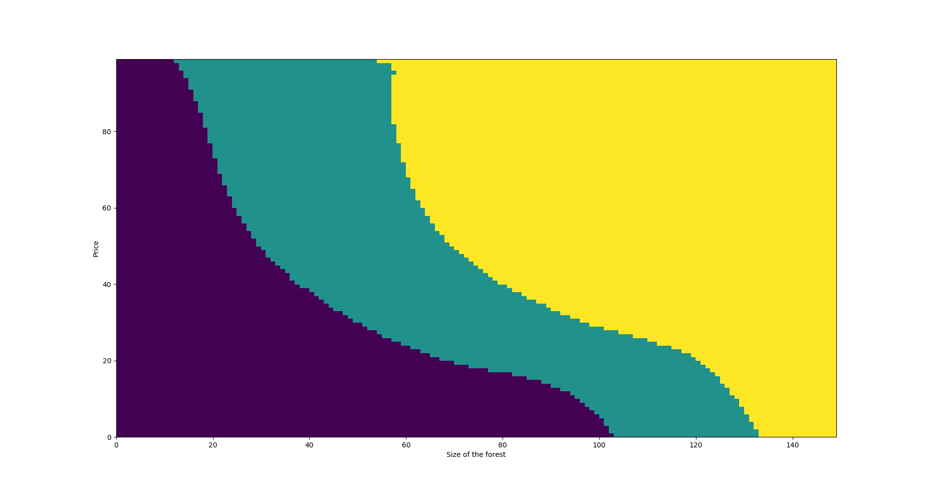
Figure 2: The optimal strategy with respect to the price $P$ and the size of the forest $R$. The blue region corresponds to the plantation region, the yellow region corresponds to the harvesting region, the green region corresponds to the continuation region

We note that the region to harvest is increasing with the price, and the region to renew is decreasing with the price. We never plant and harvest in the same time.

We now study the sensitivity w.r.t. the different parameters. For that we will change parameter by parameter.

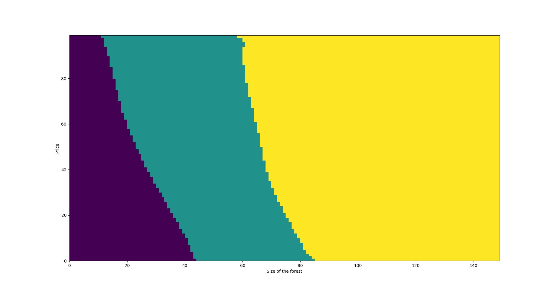
Figure 3: In this figure the parameter $\lambda$ is now $0.9$

If $\lambda$ is bigger in this case the region to harvest is more important and the region to renew is less important, since the growth is more important.

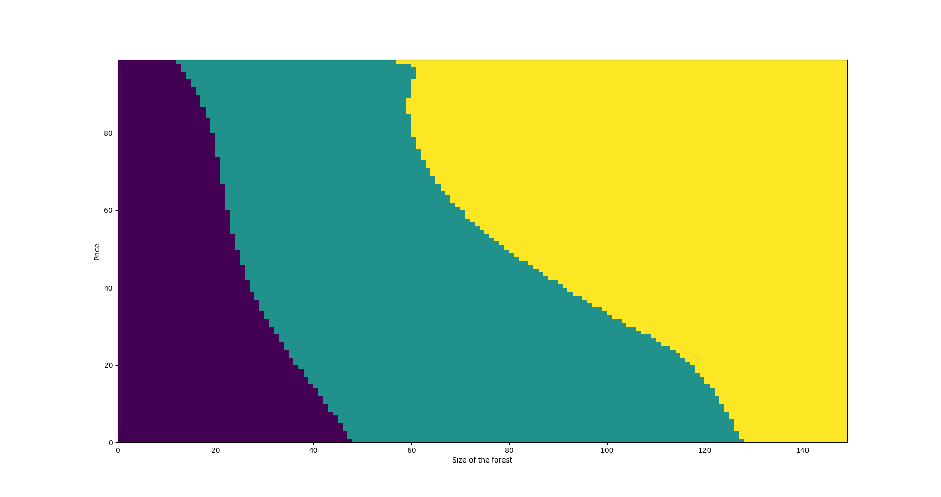
Figure 4: In this figure the parameter $\eta$ is now $0.8$

If $\eta$ is bigger in this case the region to renew is less important if the price is cheap, since the growth is slow and it is not interesting to renew except if the size of the forest is really small.

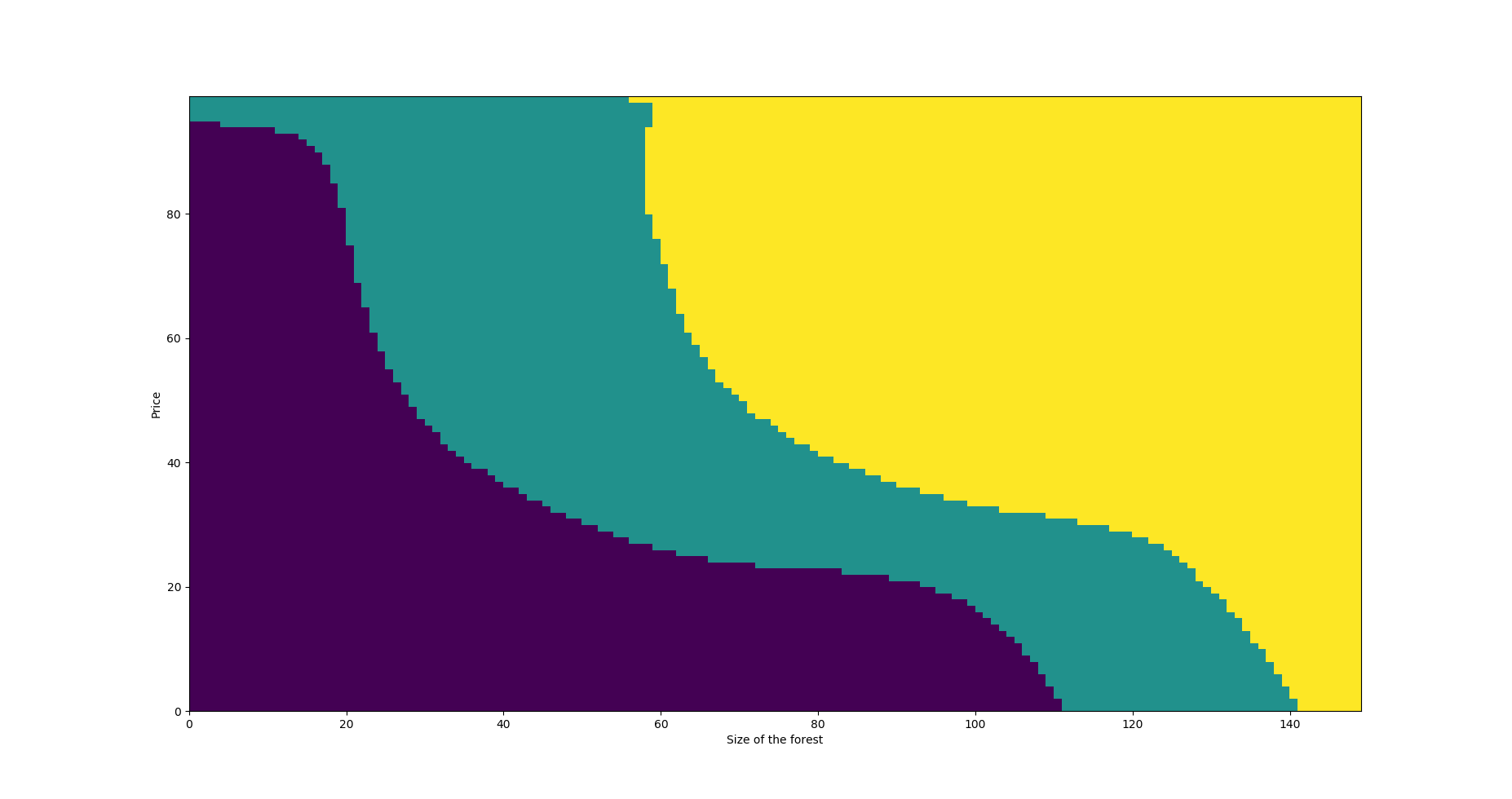
Figure 5: In this figure the drift $\mu$ of the price is now $0.09$

If the drift of the price is more important, the region to harvest is less important for a low price since the manager prefer to wait except if the size is too important because in this case the growth is negative, and the region to renew is more important because we know that the price will be better in the future.

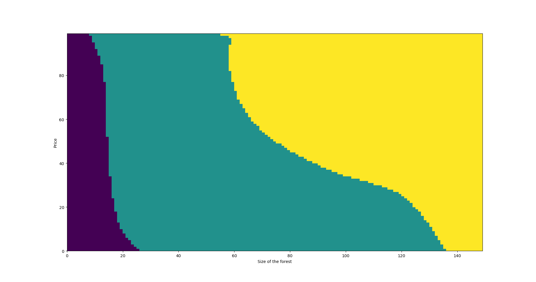
Figure 6: In this figure the proportional costs $c_{1}$ and $c_{3}$ are now $0.15$

If the costs are more expensive, the region to renew is less important because it es expensive to renew and harvest so we renew only if the size is really small.

5 Proof of the main results

5.1 Growth condition on $v$

We provide in this subsection an upper-bound for the growth of the function $v$.

For any $(t,r)\in[0,T]\times\mathbb{R}_{+}$, we define the process $\bar{R}^{t,r}$ by $\bar{R}^{t,r}_{t}=r$ and

$$d\bar{R}^{t,r}_{s} = \eta\bar{R}^{t,r}_{s}(\lambda-\bar{R}^{t,r}_{s})ds+\gamma\bar{R}^{t,r}_{s}dB_{s}\;,\quad\forall\;s\in[t,T]\setminus\{t_{i}~{}:~{}N(t)+1\leq i\leq n\}\;,$$

$$\bar{R}^{t,r}_{t_{i}} = \bar{R}^{t,r}_{t_{i}^{-}}+M\;,\quad\mbox{ for }~{}N(t)+1\leq i\leq n\;,$$

where $M:=\max_{\xi\in[0,K]}g(\xi)+g_{0}$. We remark that the process $\bar{R}^{t,r}$ can be written under the following form

$$\bar{R}^{t,r}_{s} = r+\int_{t}^{s}\eta\bar{R}^{t,r}_{u}(\lambda-\bar{R}^{t,r}_{u})du+\int_{t}^{s}\gamma\bar{R}^{t,r}_{u}dB_{u}+\big{(}N(s)-N(t)\big{)}M\;,$$

for $s\in[t,T]$. That corresponds to never harvest and renew always the maximum.

We then have the following estimate on the process $\bar{R}^{t,r}$.

Lemma 5.1.

For any $\ell\geq 1$, there exists a constant $C_{\ell}$ such that

$$\mathbb{E}\Big{[}\sup_{s\in[t,T]}\big{|}\bar{R}^{t,r}_{s}\big{|}^{\ell}\Big{]} \leq C_{\ell}\big{(}1+|r|^{\ell}\big{)}\;,$$ (5.27)

for all $(t,r)\in[0,T]\times\mathbb{R}_{+}$.

Proof. We first prove that for any $\ell\geq 1$, there exists a constant $C_{\ell}$ such that

$$\sup_{s\in[t,T]}\mathbb{E}\Big{[}\big{|}\bar{R}^{t,r}_{s}\big{|}^{\ell}\Big{]} \leq C_{\ell}\big{(}1+|r|^{\ell}\big{)}\;,$$ (5.28)

for all $(t,r)\in[0,T]\times\mathbb{R}_{+}$. We argue by induction and we prove that for each $i=N(t),\ldots,n-1$ there exists a constant $C_{\ell,i}$ such that

$$\mathbb{E}\Big{[}\big{|}\bar{R}^{t,r}_{s}\big{|}^{\ell}\Big{]} \leq C_{\ell,i}\big{(}1+|r|^{\ell}\big{)}\;,$$ (5.29)

for all $r\in\mathbb{R}_{+}$ and $s\in[t_{i}\vee t,(t_{i+1}\vee t)\wedge T)$.

$\bullet$ For $i=N(t)$, using the closed formula of the logistic diffusion, we have

$$\bar{R}^{t,r}_{s} = \frac{e^{(\eta\lambda-{\gamma^{2}\over 2})(s-t)+\gamma(B_{s}-B_{t})}}{{1\over r}+\eta\int_{t}^{s}e^{(\eta\lambda-{\gamma^{2}\over 2})(u-t)+\gamma(B_{u}-B_{t})}du}\;,$$

for all $s\in[t,t_{N(t)+1}\wedge T)$. Therefore we get

$$\mathbb{E}\Big{[}\big{|}\bar{R}^{t,r}_{s}\big{|}^{\ell}\Big{]} \leq |r|^{\ell}\mathbb{E}\Big{[}\big{|}e^{(\eta\lambda-{\gamma^{2}\over 2})(s-t)+\gamma(B_{s}-B_{t})}\big{|}^{\ell}\Big{]}$$

$$\leq |r|^{\ell}e^{(\ell|\eta\lambda-{\gamma^{2}\over 2}|+{|\ell\gamma|^{2}\over 2})(T-t)}$$

for all $s\in[t,t_{N(t)+1}\wedge T)$. Therefore (5.29) holds true.

$\bullet$ Suppose that the property holds for $i-1$. Still using the closed formula of the logistic diffusion, we have

$$\bar{R}^{t,r}_{s} = \frac{e^{(\eta\lambda-{\gamma^{2}\over 2})(s-t_{i})+\gamma(B_{s}-B_{t_{i}})}}{{1\over\bar{R}^{t,r}_{t_{i}^{-}}+M}+\eta\int_{t_{i}}^{s}e^{(\eta\lambda-{\gamma^{2}\over 2})(u-t_{i})+\gamma(B_{u}-B_{t_{i}})}du}\;,$$

for all $s\in[t_{i}\vee t,(t_{i+1}\vee t)\wedge T)$. Therefore we get

$$\mathbb{E}\Big{[}\big{|}\bar{R}^{t,r}_{s}\big{|}^{\ell}\Big{]} \leq \mathbb{E}\Big{[}\big{|}(\bar{R}^{t,r}_{t_{i}^{-}}+M)e^{(\eta\lambda-{\gamma^{2}\over 2})(s-t_{i})+\gamma(B_{s}-B_{t_{i}})}\big{|}^{\ell}\Big{]}$$

$$\leq \mathbb{E}\Big{[}\big{|}\bar{R}^{t,r}_{t_{i}^{-}}+M\big{|}^{\ell}\Big{]}e^{(\ell|\eta\lambda-{\gamma^{2}\over 2}|+{|\ell\gamma|^{2}\over 2})(T-t_{i})}$$

$$\leq C^{\prime}\Big{(}1+\mathbb{E}\Big{[}\big{|}\bar{R}^{t,r}_{t_{i}^{-}}\big{|}^{\ell}\Big{]}\Big{)}\;.$$

Using the induction assumption and Fatou’s Lemma, we get the result, and (5.29) holds true for each $i=N(t),\ldots,n$. Taking $C_{\ell}=\max_{N(t)\leq i\leq n}C_{\ell,i}$, we get (5.28).

We now prove (5.27). Still using the closed formula of the logistic diffusion we have

$$\big{|}\bar{R}^{t,r}_{s}\big{|}^{\ell} \leq \max_{N(t)\leq i\leq n}\big{|}(\bar{R}^{t,r}_{t_{i}^{-}}+M)\sup_{u\in[t_{i}\vee t,(t_{i+1}\vee t)\wedge T)}e^{(\eta\lambda-{\gamma^{2}\over 2})(u-t_{i})+\gamma(B_{u}-B_{t_{i}})}\big{|}^{\ell}$$

$$\leq \sum_{i=N(t)}^{n}\big{|}(\bar{R}^{t,r}_{t_{i}^{-}}+M)\sup_{u\in[t_{i}\vee t,(t_{i+1}\vee t)\wedge T)}e^{(\eta\lambda-{\gamma^{2}\over 2})(u-t_{i})+\gamma(B_{u}-B_{t_{i}})}\big{|}^{\ell}\;,$$

for all $s\in[t,T]$. Therefore, we get from the independence of $(B_{u}-B_{t_{i}})_{u\geq t_{i}}$ with ${\cal F}_{t_{i}}$ and (5.28)

$$\mathbb{E}\Big{[}\sup_{s\in[t,T]}\big{|}\bar{R}^{t,r}_{s}\big{|}^{\ell}\Big{]} \leq C\Big{[}\sum_{i=N(t)+1}^{n}\mathbb{E}\Big{[}\big{|}\bar{R}^{t,r}_{t_{i}^{-}}+M\big{|}^{\ell}\Big{]}+(1+|r|^{\ell})\Big{]}$$

$$\leq C^{\prime}_{\ell}(1+|r|^{\ell})\;,$$

for some constant $C^{\prime}_{\ell}$. $\Box$

Proposition 5.3.

(i) For any $\ell\geq 1$, there exists a constant $C_{\ell}$ such that

$$\mathbb{E}\Big{[}\sup_{s\in[t,T]}\big{|}R_{s}^{t,r,\alpha}\big{|}^{\ell}\Big{]} \leq C_{\ell}\big{(}1+|r|^{\ell}\big{)}$$

for any strategy $\alpha\in\hat{\cal A}_{t,z,d}$.

(ii) There exists a constant $C$ such that

$$\mathbb{E}\Big{[}\Big{(}\sum_{k\geq 1}\zeta_{k}\mathds{1}_{\tau_{k}\leq T}\Big{)}^{2}\Big{]} \leq C\big{(}1+|r|^{4}\big{)}$$

for any strategy $\alpha\in\hat{\cal A}_{t,z,d}$.

Proof. (i) Fix $\alpha=(t_{i},\xi_{i})_{N(t-\delta)+1\leq i\leq n}\cup(\tau_{k},\zeta_{k})_{k\geq 1}\in\hat{\cal A}_{t,z,d}$. Using the definition of $\bar{R}^{t,r}$ we have

$$0~{}~{}\leq~{}~{}R^{t,r,\alpha}_{s} \leq \bar{R}^{t,r}_{s}$$

for all $s\in[t,T]$. Therefore we get from Lemma 5.1

$$\mathbb{E}\Big{[}\sup_{s\in[t,T]}\big{|}R^{t,r,\alpha}_{s}\big{|}^{\ell}\Big{]} \leq \mathbb{E}\Big{[}\sup_{s\in[t,T]}\big{|}\bar{R}^{t,r}_{s}\big{|}^{\ell}\Big{]}~{}~{}\leq~{}~{}C_{\ell}\big{(}1+|r|^{\ell}\big{)}\;.$$

(ii) We turn to the second estimate. From the dynamics (2.9) of $R^{t,r,\alpha}$, and since $R_{T}^{t,r,\alpha}\geq 0$ we have

$$\sum_{k\geq 1}\zeta_{k}\mathds{1}_{\tau_{k}\leq T} \leq r+\int_{t}^{T}\eta R^{t,r,\alpha}_{u}(\lambda-R^{t,r,\alpha}_{u})du+\int_{t}^{T}\gamma R^{t,r,\alpha}_{u}dB_{u}+nM\;,$$

where we recall that $M=\max_{\xi\in[0,K]}g(\xi)+g_{0}$. Therefore, we get

$$\mathbb{E}\Big{[}\Big{(}\sum_{k\geq 1}\zeta_{k}\mathds{1}_{\tau_{k}\leq T}\Big{)}^{2}\Big{]} \leq 4\Big{(}|r|^{2}+\mathbb{E}\Big{[}\Big{|}\int_{t}^{T}\eta R^{t,r,\alpha}_{u}(\lambda-R^{t,r,\alpha}_{u})du\Big{|}^{2}+\Big{|}\int_{t}^{T}\gamma R^{t,r,\alpha}_{u}dB_{u}\Big{|}^{2}\Big{]}+n^{2}M^{2}\Big{)}\;.$$

Therefore there exists a constant $C$ depending only on $T$, $\eta$, $\lambda$, $\gamma$, $M$ and $n$ such that

$$\mathbb{E}\Big{[}\Big{(}\sum_{k\geq 1}\zeta_{k}\mathds{1}_{\tau_{k}\leq T}\Big{)}^{2}\Big{]} \leq C\Big{(}|r|^{2}+1+\mathbb{E}\Big{[}\sup_{s\in[t,T]}|R^{t,r,\alpha}_{s}|^{4}\Big{]}\Big{)}\;.$$

Using estimate (i) we get the result. $\Box$

We turn to the proof of the growth estimation for the value function $v$.

Proof of Proposition 3.2. Fix $(t,z,d)\in{\cal D}$. From the definition of the function $L$ and the dynamics (2.10) and (2.11) of $X$ and $P$ we have

$$\mathbb{E}\Big{[}L\big{(}Z^{t,z,\alpha}_{T}\big{)}\Big{]} \leq \mathbb{E}\Big{[}X^{t,z,\alpha}_{T}\Big{]}+\mathbb{E}\Big{[}\big{|}P^{t,p}_{T}\big{|}^{2}\Big{]}+\mathbb{E}\Big{[}\big{|}R^{t,r,\alpha}_{T}\big{|}^{2}\Big{]}$$

$$\leq x+\mathbb{E}\Big{[}\sup_{s\in[t,T]}|P^{t,p}_{s}|^{2}\Big{]}+\mathbb{E}\Big{[}\Big{(}\sum_{k\geq 1}\zeta_{k}\mathds{1}_{t\leq\tau_{k}\leq T}\Big{)}^{2}\Big{]}+\mathbb{E}\Big{[}\big{|}R^{t,r,\alpha}_{T}\big{|}^{2}\Big{]}$$

$$+e^{(2\mu+\sigma^{2})(T-t)}|p|^{2}$$

for any strategy $\alpha=(t_{i},\xi_{i})_{N(t-\delta)+1\leq i\leq n}\cup(\tau_{k},\zeta_{k})_{k\geq 1}\in\hat{\cal A}_{t,z,d}$. From classical estimates there exists a constant $C$ such that

$$\mathbb{E}\Big{[}\sup_{s\in[t,T]}|P^{t,p}_{s}|^{2}\Big{]} \leq C\Big{(}1+|p|^{2}\Big{)}$$

for all $p\in\mathbb{R}_{+}^{*}$. Using this estimate and Proposition 5.3 we get

$$v(t,z,d) \leq x+C\big{(}1+|r|^{4}+|p|^{4}+|q|^{4}\big{)}\;.$$

Then by considering the strategy $\alpha^{0}=d\in\hat{\cal A}_{t,z,d}$ with no more intervention than $d$, we get

$$x \leq J(t,z,\alpha^{0})~{}~{}\leq~{}~{}v(t,z,d)\;.$$

$\Box$

5.2 Dynamic programming principle

Before proving the dynamic programming principle, we need the following results.

Lemma 5.2.

For any $(t,z,d)\in{\cal D}$ and any control $\alpha\in\hat{\cal A}_{t,z,d}$ we have the following properties.

1. The pair $(Z^{t,z,\alpha},d(.,\alpha))$ satisfies the following Markov property

   $$\mathbb{E}\big{[}\phi(Z^{t,z,\alpha}_{\vartheta_{2}})\big{|}{\cal F}_{\vartheta_{1}}\big{]} = \mathbb{E}\big{[}\phi(Z^{t,z,\alpha}_{\vartheta_{2}})\big{|}(Z^{t,z,\alpha}_{\vartheta_{1}},d(\vartheta_{1},\alpha))\big{]}$$

   for any bounded measurable function $\phi$, and any $\vartheta_{1},\vartheta_{2}\in{\cal T}_{[t,T]}$ such that $\mathbb{P}\big{(}\vartheta_{1}\leq\vartheta_{2}\big{)}=1$.

2. Causality of the control

   $$\alpha^{\vartheta}\in\hat{\cal A}_{\vartheta,Z_{\vartheta}^{t,z,d},d(\vartheta,\alpha)}\quad \quad d(\vartheta,\alpha)\in D_{\vartheta}\quad a.s.$$ and

   for any $\vartheta\in{\cal T}_{[t,T]}$ where we set $\alpha^{\vartheta}=(t_{i},\xi_{i})_{N(\vartheta-\delta)+1\leq i\leq n}\cup(\tau_{k},\zeta_{k})_{k\geq\kappa(\vartheta,\alpha)+1}$ and

   $$\kappa(\vartheta,\alpha) = \#\big{\{}k\geq 1~{}:~{}\tau_{k}<\vartheta\big{\}}\;.$$

3. The state process $Z^{t,z,\alpha}$ satisfies the following flow property

   $$Z^{t,z,\alpha} = Z^{\vartheta,Z^{t,z,\alpha}_{\vartheta},\alpha^{\vartheta}}\quad\text{on }[\vartheta,T]\;,$$

   for any $\vartheta\in{\cal T}_{[t,T]}$.

Proof. These properties are direct consequences of the dynamics of $Z^{t,z,\alpha}$. $\Box$

We turn to the proof of the dynamic programming principles (DP1) and (DP2). Unfortunately, we have not enough information on the value function $v$ to directly prove these results. In particular, we do not know the measurability of $v$ and this prevents us from computing expectations involving $v$ as in (DP1) and (DP2). We therefore provide weaker dynamic programing principles involving the envelopes $v_{*}$ and $v^{*}$ as in [5]. Since we get the continuity of $v$ at the end, these results implies (DP1) and (DP2).

Proposition 5.4.

For any $(t,z,d)\in{\cal D}$ we have

$$v(t,z,d) \geq \sup_{\alpha\in\hat{\cal A}_{t,z,d}}\sup_{\vartheta\in{\cal T}_{[t,T]}}\mathbb{E}\Big{[}v_{*}(\vartheta,Z_{\vartheta}^{t,z,d},d(\vartheta,\alpha))\Big{]}\;.$$

Proof. Fix $(t,z,d)\in{\cal D}$, $\alpha\in\hat{\cal A}_{t,z,d}$ and $\vartheta\in{\cal T}_{[t,T]}$. By definition of the value function $v$, for any $\varepsilon>0$ and $\omega\in\Omega$, there exists $\alpha^{\varepsilon,\omega}\in\hat{\cal A}_{\vartheta(\omega),Z^{t,z,\alpha}_{\vartheta(\omega)}(\omega),d(\vartheta(\omega),\alpha)}$, which is an $\varepsilon$-optimal control at $(\vartheta,Z_{\vartheta}^{t,z,\alpha},d(\vartheta,\alpha))(\omega)$, i.e.

$$v\big{(}\vartheta(\omega),Z^{t,z,\alpha}_{\vartheta(\omega)}(\omega),d(\vartheta(\omega),\alpha(\omega))\big{)}-\varepsilon \leq J(\vartheta(\omega),Z^{t,z,\alpha}_{\vartheta(\omega)}(\omega),\alpha^{\varepsilon,\omega})\;.$$

By a measurable selection theorem (see e.g. Theorem 82 in the appendix of Chapter III in [12]) there exists $\bar{\alpha}_{\varepsilon}=(t_{i},\bar{\xi}_{i})_{N(\vartheta)+1\leq i\leq n}\cup(\bar{\tau}_{k},\bar{\zeta}_{k})_{k\geq 1}\in\hat{\cal A}_{\vartheta,Z^{t,z,\alpha}_{\vartheta},d(\vartheta,\alpha)}$ s.t. $\bar{\alpha}_{\varepsilon}(\omega)=\alpha_{\varepsilon,\omega}(\omega)$ a.s., and so

$$v\big{(}\vartheta,Z^{t,z,\alpha}_{\vartheta},d(\vartheta,\alpha)\big{)}-\varepsilon \leq J(\vartheta,Z^{t,z,\alpha}_{\vartheta},\bar{\alpha}_{\varepsilon})\;,\qquad\mathbb{P}-a.s.$$ (5.30)

We now define by concatenation the control strategy $\bar{\alpha}$ consisting of the impulse control components of $\alpha$ on $[t,\vartheta)$, and the impulse control components $\bar{\alpha}_{\varepsilon}$ on $[\vartheta,T]$. By construction of the control $\bar{\alpha}$ we have $\bar{\alpha}\in\hat{\cal A}_{t,z,d}$, $Z^{t,z,\bar{\alpha}}=Z^{t,z,\alpha}$ on $[t,\vartheta)$, $d(\vartheta,\bar{\alpha})=d(\vartheta,\alpha)$, and $\bar{\alpha}^{\vartheta}=\bar{\alpha}_{\varepsilon}$. From Markov property, flow property, and causality features of our model, given by Lemma 5.2, the definition of the performance criterion and the law of iterated conditional expectations, we get

$$J(t,z,\bar{\alpha}) = \mathbb{E}\Big{[}J(\vartheta,Z_{\vartheta}^{t,z,\alpha},\bar{\alpha}_{\varepsilon})\Big{]}\;.$$

Together with (5.30), this implies

$$v(t,z,d) \geq J(t,z,\bar{\alpha})$$

$$\geq \mathbb{E}\Big{[}v_{*}(\vartheta,Z^{t,z,\alpha}_{\vartheta},d(\vartheta,\alpha))\Big{]}-\varepsilon\;.$$

Since $\varepsilon$, $\vartheta$ and $\alpha$ are arbitrarily chosen, we get the result. $\Box$

We now prove (DP2), which is equivalent to the following proposition.

Proposition 5.5.

For all $(t,z,d)\in{\cal D}$, we have

$$v(t,z,d) \leq \sup_{\alpha\in\hat{\cal A}_{t,z,d}}\inf_{\vartheta\in{\cal T}_{[t,T]}}\mathbb{E}\Big{[}v^{*}\big{(}\vartheta,Z_{\vartheta}^{t,z,\alpha},d(\vartheta,\alpha)\big{)}\Big{]}\;.$$

Proof. Fix $(t,z,d)\in{\cal D}$, $\alpha\in\hat{\cal A}_{t,z,d}$ and $\vartheta\in{\cal T}_{[t,T]}$. From the definitions of the performance criterion and the value functions, the law of iterated conditional expectations, Markov property, flow property, and causality features of our model given by Lemma 5.2, we get

$$J(t,z,\alpha) = \mathbb{E}\Big{[}\mathbb{E}\Big{[}L\Big{(}Z^{\vartheta,Z^{t,z,\alpha}_{\vartheta},\alpha^{\vartheta}}_{T}\Big{)}\Big{|}{\cal F}_{\vartheta}\Big{]}\Big{]}~{}~{}=~{}~{}\mathbb{E}\Big{[}J\big{(}\vartheta,Z_{\vartheta}^{t,z,\alpha},\alpha^{\vartheta}\big{)}\Big{]}$$

$$\leq \mathbb{E}\Big{[}v^{*}\big{(}\vartheta,Z_{\vartheta}^{t,z,\alpha},d(\vartheta,\alpha)\big{)}\Big{]}\;.$$

Since $\vartheta$ and $\alpha$ are arbitrary, we obtain the required inequality. $\Box$

5.3 Viscosity properties

We first need the following comparison result. We recall that ${\cal Z}=\mathbb{R}\times\mathbb{R}_{+}\times\mathbb{R}_{+}^{*}\times\mathbb{R}_{+}^{*}$ and $D_{t}$ is given by (2.8).

Proposition 5.6.

Fix $k\in\{0,\ldots,m-1\}$ (resp. $k\in\{m,\ldots,n-1\}$) and $g:{\cal Z}\times D_{t_{k+1}}\rightarrow\mathbb{R}$ a continuous function. Let $\underline{w}:{\cal D}_{k}\rightarrow\mathbb{R}$ a viscosity subsolution to (3.18)-(3.19) and

$$\underline{w}(t_{k+1}^{-},z,d) \geq \max\big{\{}{\cal N}_{2}g(z,d)~{},~{}\bar{\cal N}_{2}g(z,d)\big{\}}\;,\quad(z,d)\in{\cal Z}\times D_{t_{k+1}}$$ (5.31)

$$\mbox{( resp. }\underline{w}(t_{k+1}^{-},z,d) \geq \max\big{\{}{\cal N}_{1}g(z,d)~{},~{}\bar{\cal N}_{1}g(z,d)\big{\}}\;,\quad(z,d)\in{\cal Z}\times D_{t_{k+1}}\mbox{ ) }\;,$$

and $\bar{w}:{\cal D}_{k}\rightarrow\mathbb{R}$ a viscosity supersolution to (3.18)-(3.19)

$$\bar{w}(t_{k+1}^{-},z,d) \leq \max\big{\{}{\cal N}_{2}g(z,d)~{},~{}\bar{\cal N}_{2}g(z,d)\big{\}}\;,\quad(z,d)\in{\cal Z}\times D_{t_{k+1}}$$ (5.32)

$$\mbox{( resp. }\bar{w}(t_{k+1}^{-},z,d) \leq \max\big{\{}{\cal N}_{1}g(z,d)~{},~{}\bar{\cal N}_{1}g(z,d)\big{\}}\;,\quad(z,d)\in{\cal Z}\times D_{t_{k+1}}\mbox{ ) }\;.$$

Suppose there exists a constant $C>0$ such that

$$\underline{w}(t,z,d) \leq x+C\big{(}1+|r|^{4}+|p|^{4}+|q|^{4}+|d|^{4}\big{)}$$ (5.33)

$$\bar{w}(t,z,d) \geq x\;,$$ (5.34)

for all $(t,z,d)\in{\cal D}_{k}$ with $z=(x,r,p,q)$. Then $\underline{w}\leq\bar{w}$ on ${\cal D}_{k}$. In particular there exists at most a unique viscosity solution $w$ to (3.18)-(3.19)-(5.31)-(5.32), satisfying (5.33)-(5.34) and $w$ is continuous on $[t_{k},t_{k+1})\times{\cal Z}$.

The proof is postponed to the end of this section. We are now able to state viscosity properties and uniqueness of $v$.

Viscosity property on ${\cal D}^{1}_{k}$.

Fix $k=0,\ldots,n-1$ and $(t,z,d)\in{\cal D}^{1}_{k}$ with $z=(x,r,p,q)$ and $r=0$.

1) We first prove the viscosity supersolution. Let $\varphi\in C^{1,2}({\cal D}_{k})$ such that

$$(v_{*}-\varphi)(t,z,d) = \min_{{\cal D}_{k}}(v_{*}-\varphi)\;.$$ (5.35)

Consider a sequence $(s_{\ell},z_{\ell},d_{\ell})_{\ell\in\mathbb{N}}$ of ${\cal D}_{k}$ such that

$$\big{(}s_{\ell},z_{\ell},d_{\ell},v(t_{\ell},z_{\ell},d_{\ell})\big{)} \xrightarrow[\ell\rightarrow+\infty]{} \big{(}t,z,d,v_{*}(t,z,d)\big{)}\;.$$

Applying Proposition 5.4 with $\vartheta=s_{\ell}+h_{\ell}$ where $h_{\ell}\in(0,s_{\ell+1}-s_{\ell})$. We have for $\ell$ large enough

$$v(s_{\ell},z_{\ell},d_{\ell}) \geq \mathbb{E}\Big{[}v_{*}(s_{\ell}+h_{\ell},Z^{\ell}_{s_{\ell}+h},d_{\ell})\Big{]}\;,$$

where $Z^{\ell}$ stands for $Z^{s_{\ell},z_{\ell},\alpha^{0}}$ with $\alpha^{0}$ the strategy with no more interventions than $d$. From (5.35), we get

$$\chi_{\ell}+\varphi(s_{\ell},z_{\ell},d_{\ell}) \geq \mathbb{E}\Big{[}\varphi(s_{\ell}+h_{\ell},Z^{\ell}_{s_{\ell}+h_{\ell}},d_{\ell})\Big{]}\;,$$

with $\chi_{\ell}:=v(s_{\ell},z_{\ell},d_{\ell})-v_{*}(t,z,d)-\varphi(s_{\ell},z_{\ell},d_{\ell})+\varphi(t,z,d)\rightarrow 0$ as $\ell\rightarrow\infty$. Taking $h_{\ell}=\sqrt{|\chi_{\ell}|}$ and applying Ito’s formula we get

$${1\over h_{\ell}}\mathbb{E}\Big{[}\int_{s_{\ell}}^{s_{\ell}+h_{\ell}}-{\cal L}\varphi(s,Z^{\ell}_{s},d_{\ell})ds\Big{]} \geq -\sqrt{|\chi_{\ell}|}\;.$$

Sending $\ell$ to $\infty$, we get the supersolution property from the mean value theorem.

2) We turn to the viscosity subsolution. Let $\varphi\in C^{1,2}({\cal D}_{k})$ such that

$$(v^{*}-\varphi)(t,z,d) = \max_{{\cal D}_{k}}(v^{*}-\varphi)\;.$$ (5.36)

Consider a sequence $(s_{\ell},z_{\ell},d_{\ell})_{\ell\in\mathbb{N}}$ of ${\cal D}_{k}$ such that

$$\big{(}s_{\ell},z_{\ell},d_{\ell},v(s_{\ell},z_{\ell},d_{\ell})\big{)} \xrightarrow[\ell\rightarrow+\infty]{} \big{(}t,z,d,v^{*}(t,z,d)\big{)}\;.$$

From Proposition 5.5 we can find for each $\ell\in\mathbb{N}$ a control $\alpha^{\ell}=(t_{i},\xi^{\ell}_{i})_{N(t_{\ell}-\delta)+1\leq i\leq n}\cup(\tau_{k},\zeta_{k})_{k\geq 1}\in\hat{\cal A}_{s_{\ell},z_{\ell},d_{\ell}}$ such that

$$v(s_{\ell},z_{\ell},d_{\ell}) \leq \mathbb{E}\Big{[}v^{*}(s_{\ell}+h_{\ell},Z^{\ell}_{s_{\ell}+h_{\ell}},d)\Big{]}+{1\over\ell}\;,$$

where $Z^{\ell}$ stands for $Z^{s_{\ell},z_{\ell},\alpha^{\ell}}$ and $h_{\ell}\in(0,s_{\ell+1}-t_{\ell})$ is a constant that will be chosen later.

We first notice that

$$\sup_{s\in[s_{\ell},s_{\ell}+h_{\ell}]}|R^{\ell}_{s}| \xrightarrow[\ell\rightarrow\infty]{\mathbb{P}-a.s.} 0\;.$$ (5.37)

Indeed, we have

$$0~{}~{}\leq~{}~{}R^{\ell}_{s} \leq \bar{R}^{\ell}_{s}\;,\quad s\geq s_{\ell}$$ (5.38)

where $\bar{R}^{\ell}$ is given by

$$\bar{R}^{\ell}_{s} = r_{\ell}+\int_{s_{\ell}}^{s}\eta\bar{R}^{\ell}_{u}(\lambda-\bar{R}^{\ell}_{u})du+\int_{s_{\ell}}^{s}\bar{R}^{\ell}_{u}dB_{u}\;,\quad s\geq s_{\ell}\;.$$

Since $r_{\ell}\xrightarrow[\ell\rightarrow\infty]{}r$ (and $r=0$), we have $\sup_{s\in[s_{\ell},s_{\ell}+h_{\ell}]}|\bar{R}^{\ell}_{s}|\xrightarrow[\ell\rightarrow\infty]{}0$ as $\ell\rightarrow\infty$ and we get (5.37). In particular, we deduce that up to a subsequence

$$\sum_{k\geq 1}\zeta_{k}^{\ell}\mathds{1}_{\tau_{k}^{\ell}\leq s_{\ell}+h_{\ell}} \xrightarrow[\ell\rightarrow+\infty]{\mathbb{P}-a.s.} 0\;.$$ (5.39)

Indeed, we have from (2.9) and (5.38)

$$\sum_{k\geq 1}\zeta_{k}^{\ell}\mathds{1}_{\tau_{k}^{\ell}\leq s_{\ell}+h_{\ell}} \leq r_{\ell}+\int_{s_{\ell}}^{s_{\ell}+h_{\ell}}\eta\lambda R^{\ell}_{u}du+\int_{s_{\ell}}^{s_{\ell}+h_{\ell}}\eta R^{\ell}_{u}dB_{u}$$

$$\leq r_{\ell}+h_{\ell}\eta\lambda\sup_{s\in[s_{\ell},s_{\ell}+h_{\ell}]}|\bar{R}^{\ell}_{s}|+\big{|}\int_{s_{\ell}}^{s_{\ell}+h_{\ell}}\eta R^{\ell}_{u}dB_{u}\big{|}\;.$$

From BDG inequality and (5.38), we get from (5.37)

$$\mathbb{E}\Big{[}\big{|}\int_{s_{\ell}}^{s_{\ell}+h_{\ell}}\eta R^{\ell}_{u}dB_{u}\big{|}\big{]} \xrightarrow[\ell\rightarrow+\infty]{} 0\;,$$

and hence, up to a subsequence $\big{|}\int_{s_{\ell}}^{s_{\ell}+h_{\ell}}\eta R^{\ell}_{u}dB_{u}\big{|}\rightarrow 0$ as $\ell\rightarrow+\infty$. From this convergence (5.37) and (5.3), we get (5.39).

We then define the process $\tilde{X}^{\ell}$ by

$$\tilde{X}^{\ell}_{s} = x_{\ell}+\sum_{k\geq 1}P_{\tau_{k}^{\ell}}\zeta_{k}^{\ell}\mathds{1}_{\tau_{k}^{\ell}\leq s}$$

and observe that from (5.39)

$$\tilde{X}^{\ell}_{s_{\ell}+h_{\ell}} \xrightarrow[\ell\rightarrow+\infty]{\mathbb{P}-a.s.} x\;,$$ (5.40)

$$\tilde{X}^{\ell} \geq X^{\ell}\;.$$

Since $v$ is nondecreasing in the $x$ component, it is the same for $v^{*}$. We get

$$v(s_{\ell},z_{\ell},d_{\ell}) \leq \mathbb{E}\Big{[}v^{*}(s_{\ell}+h_{\ell},\tilde{Z}^{\ell}_{s_{\ell}+h_{\ell}},d)\Big{]}+{1\over\ell}$$

where $\tilde{Z}^{\ell}=(\tilde{X}^{\ell},R^{\ell},P^{\ell},Q^{\ell})$. We then get from (5.36)

$$\chi_{\ell}+\varphi(s_{\ell},z_{\ell},d_{\ell}) \leq \mathbb{E}\Big{[}\varphi(s_{\ell}+h,\tilde{Z}^{\ell}_{s_{l}+h},d_{\ell})\Big{]}+{1\over\ell}\;,$$

where $\chi_{\ell}:=v(s_{\ell},z_{\ell},d_{\ell})-v^{*}(t,z,d)-\varphi(s_{\ell},z_{\ell},d_{\ell})+\varphi(t,z,d)\rightarrow 0$ as $\ell\rightarrow+\infty$. Applying Ito’s formula and taking $h_{\ell}=\sqrt{|\chi_{\ell}|}$ we get by sending $\ell$ to $\infty$ as previously

$$-{\cal L}\varphi(t,z,d) \leq 0\;.$$

Viscosity property on ${\cal D}^{2}_{k}$.

Fix $k=0,\ldots,n-1$ and $(t,z,d)\in{\cal D}^{2}_{k}$. Then $v(.,d)$ is the value function associated to an optimal impulse control problem with nonlocal operator ${\cal H}$. Using the same arguments as in the proof of Theorem 5.1 in [18], we obtain that $v$ is a viscosity solution to (3.19) on ${\cal D}_{k}^{2}$.

Viscosity property and continuity on $\{t_{k}\}\times{\cal Z}\times D_{t_{k}}$.

We prove it by a backward induction on $k=0,\ldots,n$.

$\bullet$ Suppose that $k=n$ $i.e.$ $t_{k}=T$.

1) We first prove the subsolution property. Fix some $z=(x,r,p,q)\in{\cal Z}$ and $d=(t_{i},e_{i})_{n-m+1\leq i\leq n}\in D_{t_{n}}$ and consider a sequence $(s_{\ell},z_{\ell},d_{\ell})_{\ell\in\mathbb{N}}$ with $z_{\ell}=(x_{\ell},r_{\ell},p_{\ell},q_{\ell})$ and $d_{\ell}=(t_{i},e_{i}^{\ell})_{n-m+1\leq i\leq n}$ such that

$$(s_{\ell},z_{\ell},d_{\ell},v(s_{\ell},z_{\ell},d_{\ell})) \xrightarrow[\ell\rightarrow+\infty]{} (T^{-},z,d,v_{*}(T^{-},z,d))\;.$$

By considering a strategy $\alpha^{\ell}\in\hat{\cal A}_{s_{\ell},z_{\ell},d_{\ell}}$ with a single renewing order $(T,e)$ with $e\leq K$ and the stopping time $\vartheta=T$, we get from the definition of $v$

$$v(s_{\ell},z_{\ell},d_{\ell}) \geq \mathbb{E}\Big{[}L\Big{(}\Gamma^{rn}_{1}\big{(}\Gamma^{rn}_{2}(Z^{s_{\ell},z_{\ell},\alpha^{\ell}}_{T^{-}},e^{\ell}_{n-m+1}),e\big{)}\Big{)}\Big{]}\;.$$

From the continuity of the functions $L$, $\Gamma^{rn}_{1}$ and $\Gamma^{rn}_{2}$, we get

$$L\Big{(}\Gamma^{rn}_{1}\big{(}\Gamma^{rn}_{2}(Z^{s_{\ell},z_{\ell},\alpha^{\ell}}_{T^{-}},e^{\ell}_{n-m+1}),e\big{)} \xrightarrow[\ell\rightarrow+\infty]{\mathbb{P}-a.s.} L\Big{(}\Gamma^{rn}_{1}\big{(}\Gamma^{rn}_{2}(z,e_{n-m+1}),e\big{)}\;.$$

From Fatou’s Lemma and since $e\leq K$ is arbitrarily chosen, we get by sending $\ell$ to $\infty$

$$v_{*}(T^{-},z,d) \geq {\cal N}_{1}L(z,d)\;.$$ (5.41)

Fix now $a\in[0,r]$ and denote $a_{\ell}=\min\{a,r_{\ell}\}$. By considering a strategy $\alpha^{\ell}$ with an immediate harvesting order $(s_{\ell},r_{\ell})$ and a single renewing order $(T,e)$ and $\vartheta=T$, we get from the definition of $v$

$$v(s_{\ell},z_{\ell},d_{\ell}) \geq \mathbb{E}\Big{[}L\Big{(}\Gamma^{rn}_{1}\big{(}\Gamma^{rn}_{2}\big{(}Z^{s_{\ell},\Gamma^{c}(z_{\ell},r_{\ell}),\alpha^{\ell}}_{T^{-}},e_{n-m+1}\big{)},e\big{)}\Big{)}\Big{]}\;.$$

From the continuity of the functions $L$, $\Gamma^{c}$, $\Gamma^{rn}_{1}$ and $\Gamma^{rn}_{2}$, we get

$$L\Big{(}\Gamma^{rn}_{1}\big{(}\Gamma^{rn}_{2}\big{(}Z^{s_{\ell},\Gamma^{c}(z_{\ell},r_{\ell}),\alpha^{\ell}}_{T^{-}},e_{n-m+1}\big{)},e\big{)}\Big{)} \xrightarrow[\ell\rightarrow+\infty]{\mathbb{P}-a.s.} L\Big{(}\Gamma^{rn}_{1}\big{(}\Gamma^{rn}_{2}\big{(}\Gamma^{c}(z,r),e_{n-m+1}\big{)},e\big{)}\Big{)}\;.$$

From Fatou’s Lemma and since $e\leq K$ and $a\in[0,r]$ are arbitrarily chosen, we get by sending $\ell$ to $\infty$

$$v_{*}(T^{-},z,d) \geq \bar{\cal N}_{1}L(z,d)\;.$$ (5.42)

From (5.41) and (5.42), we get the subsolution property at $(T^{-},z,d)$.

2) We turn to the supersolution property. We argue by contradiction and suppose that there exist $z=(x,r,p,q)\in{\cal Z}$ and $d\in D_{t_{n}}$ such that

$$v^{*}(T^{-},z,d) \geq \max\Big{\{}{\cal N}_{1}L(z,d)~{},~{}\bar{\cal N}_{1}L(z,d)\Big{\}}+2\varepsilon\;,$$

with $\varepsilon>0$. We fix a sequence $(s_{\ell},z_{\ell},d_{\ell})_{\ell\in\mathbb{N}}$ in ${\cal D}$ such that

$$(s_{\ell},z_{\ell},d_{\ell},v(s_{\ell},z_{\ell},d_{\ell})) \xrightarrow[\ell\rightarrow+\infty]{} (T^{-},z,d,v^{*}(T^{-},z,d))\;.$$ (5.43)

We then can find $s>0$ and a sequence of smooth functions $(\varphi^{h})_{h\geq 1}$ on $[T-s,T]\times{\cal Z}\times D_{t_{n}}$ such that $\varphi^{h}\downarrow v^{*}$ on $[T-s,T)\times{\cal Z}\times D_{t_{n}}$, $\varphi^{h}\downarrow v^{*}(.^{-},.,.)$ on $\{T\}\times{\cal Z}\times D_{t_{n}}$ as $h\uparrow+\infty$ and

$$\varphi^{h}(t^{\prime},z^{\prime},d^{\prime}) \geq \max\Big{\{}{\cal N}_{1}L(z^{\prime},d^{\prime})~{},~{}\bar{\cal N}_{1}L(z^{\prime},d^{\prime})\Big{\}}+\varepsilon\;,$$ (5.44)

on some neighborhood ${\cal B}^{h}$ of $(T,z,d)$ in $[t_{n},T]\times{\cal Z}\times D_{t_{n}}$. Up to a subsequence, we can assume that ${\cal B}^{h}_{\ell}:=[t_{\ell},T]\times B((z_{\ell},d_{\ell}),\delta_{\ell}^{h})\subset{\cal B}^{h}$ for $\delta_{\ell}^{h}$ sufficiently small. Since $v^{*}$ is locally bounded, there is some $\iota>0$ such that $|v^{*}|\leq\iota$ on ${\cal B}^{h}$. We therefore get $\varphi^{h}\geq-\iota$ on ${\cal B}^{h}$. We then define the function $\varphi^{h}_{\ell}$ by

$$\varphi^{h}_{\ell}(t^{\prime},z^{\prime},d^{\prime}) = \varphi^{h}(t^{\prime},z^{\prime},d^{\prime})+3\iota{|(z^{\prime},d^{\prime})-(z_{\ell},d_{\ell})|^{2}\over|\delta^{h}_{\ell}|^{2}}+\sqrt{T-t^{\prime}}\;,$$

and we observe that

$$(v^{*}-\varphi_{\ell}^{h}) \leq -\iota~{}~{}<~{}~{}0\quad\mbox{ on }[t_{\ell},T]\times\partial B((z_{\ell},d_{\ell}),\delta_{\ell}^{h})\;.$$ (5.45)

Since ${\partial\sqrt{T-t}\over\partial t}\rightarrow-\infty$ as $t\rightarrow T^{-}$, we can choose $h$ large enough such that

$$-{\cal L}\varphi_{\ell}^{h} \geq 0~{}\mbox{ on }~{}{\cal B}_{\ell}^{h}\;.$$ (5.46)

From the definition of $v$ we can find $\alpha^{\ell}=(t_{i},\xi_{i}^{\ell})_{N(t_{\ell}-\delta)+1\leq i\leq n}\cup(\tau_{k}^{\ell},\zeta_{k}^{\ell})_{k\geq 1}\in\hat{\cal A}_{s_{\ell},z_{\ell},d_{\ell}}$ such that

$$v(t_{\ell},z_{\ell},d_{\ell}) \leq \mathbb{E}\Big{[}L\big{(}Z^{\ell}_{T}\big{)}\Big{]}+{1\over\ell}\;,$$ (5.47)

where $Z^{\ell}$ stands for $Z^{s_{\ell},z_{\ell},\alpha^{\ell}}$. Denote by $\theta_{\ell}^{h}=\inf\{s\geq s_{\ell}~{}:~{}(s,Z^{\ell},d_{\ell})\notin{\cal B}_{\ell}^{h}\}\wedge\tau^{\ell}_{1}$. From Ito’s formula, (5.44), (5.45) and (5.46) we have

$$\varphi_{\ell}^{h}(s_{\ell},z_{\ell},d_{\ell}) \geq \mathbb{E}\Big{[}\Big{(}v\big{(}T,\Gamma^{rn}(\Gamma^{c}(Z^{\ell}_{T^{-}},\zeta_{1}^{\ell}),\xi_{n-m}^{\ell}),d_{\ell}\cup(t_{n-m},\xi^{\ell}_{n-m})\big{)}\mathds{1}_{\tau_{1}^{\ell}=T}$$

$$\qquad+v^{*}\big{(}\theta^{\ell}_{n},\Gamma^{c}(Z^{\ell}_{{\theta_{\ell}^{h}}^{-}},\zeta_{1}^{\ell}),d_{\ell})\big{)}\mathds{1}_{\tau_{1}^{\ell}<T}\Big{)}\mathds{1}_{\tau^{\ell}_{1}\leq\theta_{\ell}^{h}}\Big{]}$$

$$+\mathbb{E}\Big{[}\Big{(}v\big{(}T,\Gamma^{rn}(Z^{\ell}_{T^{-}},\xi^{\ell}_{n-m}),d_{\ell}\cup(t_{n-m},\xi^{\ell}_{n-m})\big{)}\mathds{1}_{\theta_{\ell}^{h}=T}$$

$$\qquad+v^{*}\big{(}\theta_{\ell}^{h},Z^{\ell}_{{\theta_{\ell}^{h}}^{-}},d_{\ell}\big{)}\mathds{1}_{\theta_{\ell}^{h}<t_{k}}\Big{)}\mathds{1}_{\tau^{1}_{\ell}>\theta_{\ell}^{h}}\Big{]}+\varepsilon\wedge\iota\;.$$

From (5.47) and the Markov property given by Lemma 5.2 (i), we get by taking the conditional expectation given ${\cal F}_{\theta_{\ell}^{h}}$,

$$v(t_{\ell},z_{\ell},d_{\ell}) \leq \mathbb{E}\Big{[}\Big{(}v\big{(}T,\Gamma^{rn}(\Gamma^{c}(Z^{\ell}_{T^{-}},\zeta_{1}^{\ell}),\xi_{k}^{\ell}),d_{\ell}\cup(t_{n-m},\xi^{\ell}_{n-m})\big{)}\mathds{1}_{\tau_{1}^{\ell}=T}$$

$$\qquad+v^{*}\big{(}\theta_{\ell}^{h},\Gamma^{c}(Z^{\ell}_{{\theta_{\ell}^{h}}^{-}},\zeta_{1}^{\ell}),d_{\ell})\big{)}\mathds{1}_{\tau_{1}^{\ell}<T}\Big{)}\mathds{1}_{\tau^{\ell}_{1}\leq\theta_{\ell}^{h}}\Big{]}$$

$$+\mathbb{E}\Big{[}\Big{(}v\big{(}T,\Gamma^{rn}(Z^{\ell}_{T^{-}},\xi^{\ell}_{n-m}),d_{\ell}\cup(t_{n-m},\xi^{\ell}_{n-m})\big{)}\mathds{1}_{\theta_{\ell}^{h}=T}$$

$$\qquad+v^{*}\big{(}\theta_{\ell}^{h},Z^{\ell}_{{\theta_{\ell}^{h}}^{-}},d_{\ell}\big{)}\mathds{1}_{\theta_{\ell}^{h}<T}\Big{)}\mathds{1}_{\tau_{1}^{\ell}>\theta_{\ell}^{h}}\Big{]}+{1\over\ell}\;.$$

We therefore get

$$\varphi^{h}(s_{\ell},z_{\ell},d_{\ell})+\sqrt{T-s_{\ell}}~{}~{}=~{}~{}\varphi_{\ell}^{h}(s_{\ell},z_{\ell},d_{\ell}) \geq v(s_{\ell},z_{\ell},d_{\ell})+\varepsilon\wedge\iota-{1\over\ell}\;.$$

Sending $\ell$ and $h$ to $+\infty$ we get a contradiction with (5.43).

$\bullet$ Suppose that the property holds true for $k+1$. From Proposition 5.6, the function $v$ is continuous on $D_{t_{k+1}}$. Therefore, we get from Propositions 5.4 and 5.5

$$v(t,z,d) = \sup_{\alpha\in\hat{\cal A}_{t,z,d}}\mathbb{E}\Big{[}v\big{(}t_{k+1},Z^{t,z,\alpha}_{t_{k+1}},d(t_{k+1},\alpha)\big{)}\Big{]}$$

for all $(t,z,d)\in{\cal D}_{k}$.

We can then apply the same arguments as for $k=n$ and we get the viscosity property at $(t_{k+1}^{-},z,d)$ for all $(z,d)\in{\cal Z}\times D_{t_{k+1}}$.

Proof of Proposition 5.6.

We fix the functions $\underline{w}$ and $\bar{w}$ as in the statement of Proposition 5.6. We then introduce as classically done a perturbation of $\bar{w}$ to make it a strict supersolution.

Lemma 5.3.

Consider the function $\psi$ defined by

$$\psi(t,z,d) = x+pr+\tilde{C}_{1}e^{-\tilde{C}_{2}t}\big{(}1+|r|^{4}+|p|^{4}+|q|^{4}+|d|^{4}\big{)}\;,$$

where $\tilde{C}_{1}$ and $\tilde{C}_{2}$ are two positive constants and define for $m\geq 1$ the function $\bar{w}_{m}$ on ${\cal D}_{k}$ by

$$\bar{w}_{m} = \bar{w}+{1\over m}\psi\;.$$

Then there exist $\tilde{C}_{1}$ and $\tilde{C}_{2}$ (large enough) such that the following properties hold.

• The function $\bar{w}_{m}$ is a strict viscosity supersolution to (3.18)-(3.19) on $[t_{k},t_{k+1})\times{\cal K}$ for any compact subset ${\cal K}$ of ${\cal Z}\times D_{t_{k}}$ and any $m\geq 1$ : there exists a constant $\delta>0$ (depending on ${\cal K}$ and $m$) such that

  $$-{\cal L}\varphi(t,z,d)\geq\delta$$

  $$\mbox{(resp. }\min\Big{\{}-{\cal L}\varphi(t,z,d)~{},~{}\bar{w}_{m}(t,z,d)-{\cal H}\bar{w}_{m}(t,z,d)\Big{\}}\geq\delta\mbox{)}$$

  for any $(t,z,d)\in{\cal D}_{k}^{1}$ (resp. $(t,z,d)\in{\cal D}_{k}^{2}$) and $\varphi\in C^{1,2}({\cal D}_{k})$ such that $(z,d)\in{\cal K}$ and

  $$(\bar{w}_{m}-\varphi)(t,z,d) = \min_{{\cal D}_{k}}(\bar{w}_{m}-\varphi)\;.$$

• We have

  $$\lim_{|(z,d)|\rightarrow+\infty}(\underline{w}-\bar{w}_{m})(t,z,d) = -\infty\;.$$ (5.48)

Proof. A straightforward computation shows that

$$\psi-{\cal H}\psi \geq c_{2}>0\;,$$

on ${\cal D}_{k}$. Since $\bar{w}$ is a viscosity supersolution to (3.19), we get

$$\bar{w}_{m}-{\cal H}\bar{w}_{m} \geq {c_{2}\over m}~{}~{}=:~{}~{}\delta_{0}~{}~{}>~{}~{}0\;,$$ (5.49)

on ${\cal D}^{2}_{k}$. Then, from the definition of the operator ${\cal L}$ we get for $\tilde{C}_{2}$ large enough

$$-{\cal L}\psi > 0\quad\mbox{ on }{\cal D}_{t_{k}}\;.$$

In particular, since $-{\cal L}\psi$ is continuous, we get

$$\inf_{[t_{k},t_{k+1})\times{\cal K}}-{1\over m}{\cal L}\psi~{}~{}=:~{}~{}\delta_{1} > 0$$ (5.50)

for any compact subset ${\cal K}$ of ${\cal Z}\times D_{t_{k}}$. By writing the viscosity supersolution property of $\bar{w}$, we deduce from (5.49) and (5.50) the desired strict viscosity supersolution property for $w_{m}$.

Finally, from growth conditions (5.33) and (5.34), we get (5.48) for $\tilde{C}_{1}$ large enough. $\Box$

To prove the comparison result, it suffices to prove that

$$\sup_{{\cal D}_{k}}\;(\underline{w}-\bar{w}_{m}) \leq 0\;,$$

for all $m\geq 1$. We argue by contradiction and suppose that there exists $m\geq 1$ such that

$$\bar{\Delta}~{}~{}:=~{}~{}\sup_{{\cal D}_{k}}\;(\underline{w}-\bar{w}_{m}) > 0\;.$$

Since $\bar{w}_{m}-\underline{w}$ is u.s.c. on ${\cal D}_{k}$ and $\bar{w}_{m}-\underline{w}(t_{k+1}^{-},.)\leq 0$, we get from (5.48) the existence of an open subset ${\cal O}$ of ${\cal Z}\times D_{t_{k}}$ and $(t_{0},z_{0},d_{0})\in[t_{k},t_{k+1})\times{\cal O}$ such that $\bar{\cal O}$ is compact and

$$(\underline{w}-\bar{w}_{m})(t_{0},z_{0},d_{0}) = \bar{\Delta}\;.$$

We then consider the functions $\Phi_{i}$ and $\Theta_{i}$ defined on $[t_{k},t_{k+1})\times\bar{\cal O}$ by

$$\Phi_{i}(t,t^{\prime},z,z^{\prime},d,d^{\prime}) = \underline{w}(t,z,d)-\bar{w}_{m}(t^{\prime},z^{\prime},d^{\prime})-\Theta_{i}(t,t^{\prime},z,z^{\prime},d,d^{\prime})$$

$$\Theta_{i}(t,t^{\prime},z,z^{\prime},d,d^{\prime}) = |t-t_{0}|^{2}+|z-z_{0}|^{4}+|d-d_{0}|^{2}+{i\over 2}\big{(}|z-z^{\prime}|^{2}+|d-d^{\prime}|^{2}\big{)}$$

for all $(t,z,d),(t^{\prime},z^{\prime},d^{\prime})\in D_{k}$ and $i\geq 1$. From the growth properties of $\underline{w}$ and $\bar{w}_{m}$, there exists $(\hat{t}_{i},\hat{t}^{\prime}_{i},\hat{z}_{i},\hat{z}^{\prime}_{i},\hat{d}_{i},\hat{d}^{\prime}_{i})\in([t_{k},t_{k+1})\times\bar{\cal O})^{2}$ such that

$$\bar{\Delta}_{i} := \sup_{[t_{k},t_{k+1})\times\bar{\cal O}}\Phi_{i}~{}~{}=~{}~{}\Phi_{i}(\hat{t}_{i},\hat{t}^{\prime}_{i},\hat{z}_{i},\hat{z}^{\prime}_{i},\hat{d}_{i},\hat{d}^{\prime}_{i})\;.$$

By classical arguments we get, up to a subsequence, the following convergences

$$\big{(}\hat{t}_{i},\hat{t}^{\prime}_{i},\hat{z}_{i},\hat{z}^{\prime}_{i},\hat{d}_{i},\hat{d}^{\prime}_{i},\big{)} \xrightarrow[i\rightarrow+\infty]{} \big{(}t_{0},t_{0},z_{0},z_{0},d_{0},d_{0},\big{)}\;,$$

$$\Phi_{i}(\hat{t}_{i},\hat{t}^{\prime}_{i},\hat{z}_{i},\hat{z}^{\prime}_{i},\hat{d}_{i},\hat{d}^{\prime}_{i}) \xrightarrow[i\rightarrow+\infty]{} (\underline{w}-\bar{w}_{m})(t_{0},z_{0},d_{0})\;,$$

$$\Theta_{i}(\hat{t}_{i},\hat{t}^{\prime}_{i},\hat{z}_{i},\hat{z}^{\prime}_{i},\hat{d}_{i},\hat{d}^{\prime}_{i}) \xrightarrow[i\rightarrow+\infty]{} 0\;.$$ (5.51)

In particular, we have $\max\{\hat{t}_{i},\hat{t}_{i}^{\prime}\}<T$ for $i$ large enough. We then apply Ishii’s Lemma (see Theorem 8.3 in [10]) to $(\hat{t}_{i},\hat{t}^{\prime}_{i},\hat{z}_{i},\hat{z}^{\prime}_{i},\hat{d}_{i},\hat{d}^{\prime}_{i})$ which realizes the maximum of $\Phi_{i}$ and we get for any $\varepsilon_{i}>0$, the existence of $(e_{i},f_{i},M_{i})\in\bar{J}^{2,+}\underline{w}(\hat{t}_{i},\hat{z}_{i})$ and $(e^{\prime}_{i},f^{\prime}_{i},M^{\prime}_{i})\in\bar{J}^{2,-}\bar{w}_{m}(\hat{t}^{\prime}_{i},\hat{z}^{\prime}_{i})$ such that

$$e_{i}~{}~{}=~{}~{}{\partial\Theta_{i}\over\partial t}(\hat{t}_{i},\hat{t}^{\prime}_{i},\hat{z}_{i},\hat{z}^{\prime}_{i},\hat{d}_{i},\hat{d}^{\prime}_{i}) f_{i}~{}~{}=~{}~{}{\partial\Theta_{i}\over\partial z}(\hat{t}_{i},\hat{t}^{\prime}_{i},\hat{z}_{i},\hat{z}^{\prime}_{i},\hat{d}_{i},\hat{d}^{\prime}_{i})$$ (5.52)

$$e_{i}^{\prime}~{}~{}=~{}~{}{\partial\Theta_{i}\over\partial t^{\prime}}(\hat{t}_{i},\hat{t}^{\prime}_{i},\hat{z}_{i},\hat{z}^{\prime}_{i},\hat{d}_{i},\hat{d}^{\prime}_{i}) f_{i}^{\prime}~{}~{}=~{}~{}{\partial\Theta_{i}\over\partial z^{\prime}}(\hat{t}_{i},\hat{t}^{\prime}_{i},\hat{z}_{i},\hat{z}^{\prime}_{i},\hat{d}_{i},\hat{d}^{\prime}_{i})$$ (5.53)

and

$$\left(\begin{array}[]{cc}M&0\\ 0&-M^{\prime}\end{array}\right)~{}~{}\leq~{}~{}{\partial^{2}\Theta_{i}\over\partial(z,z^{\prime})^{2}}(\hat{t}_{i},\hat{t}^{\prime}_{i},\hat{z}_{i},\hat{z}^{\prime}_{i},\hat{d}_{i},\hat{d}^{\prime}_{i})+{1\over i}\Big{(}{\partial^{2}\Theta_{i}\over\partial(z,z^{\prime})^{2}}(\hat{t}_{i},\hat{t}^{\prime}_{i},\hat{z}_{i},\hat{z}^{\prime}_{i},\hat{d}_{i},\hat{d}^{\prime}_{i})\Big{)}^{2}\;,$$ (5.54)

for all $i\geq 1$. We then distinguish two cases.

$\bullet$ Case 1: there exists a subsequence of $(\hat{t}_{i},\hat{t}^{\prime}_{i},\hat{z}_{i},\hat{z}^{\prime}_{i},\hat{d}_{i},\hat{d}^{\prime}_{i})_{i\in\mathbb{N}}$ still denoted $(\hat{t}_{i},\hat{t}^{\prime}_{i},\hat{z}_{i},\hat{z}^{\prime}_{i},\hat{d}_{i},\hat{d}^{\prime}_{i})_{i\in\mathbb{N}}$ such that

$$(\hat{t}_{i},\hat{z}_{i},\hat{d}_{i}) \in {\cal D}_{k}^{2}\quad\mbox{ for all }~{}i\geq 1\;.$$

From the viscosity subsolution property of $\underline{w}$ and the strict viscosity supersolution property of $\bar{w}_{m}$ we have

$$\min\Big{\{}-{\cal L}[\hat{z}_{i},\hat{d}_{i},e_{i},f_{i},M_{i}]~{};~{}(\underline{w}-{\cal H}\underline{w})(\hat{t}_{i},\hat{z}_{i},\hat{d}_{i})\Big{\}} \leq 0$$ (5.55)

$$\min\Big{\{}-{\cal L}[\hat{z}^{\prime}_{i},\hat{d}^{\prime}_{i},e^{\prime}_{i},f_{i}^{\prime},M_{i}^{\prime}]~{};~{}(\bar{w}_{m}-{\cal H}\bar{w}_{m})(\hat{t}_{i},\hat{z}_{i},\hat{d}_{i})\Big{\}} \geq \delta\over m$$ (5.56)

where

$${\cal L}[z,d,e,f,M] = e+\mu pf_{3}+\rho qf_{4}+\eta r(\lambda-r)f_{2}$$

$$+{1\over 2}\Big{(}\sigma^{2}p^{2}M_{3,3}+\varsigma^{2}q^{2}M_{4,4}+2\sigma\varsigma pqM_{3,4}+\gamma^{2}r^{2}M_{2,2}\Big{)}$$

for any $z\in{\cal Z}$, $d\in D_{t_{k}}$, $e\in\mathbb{R}$, $f\in\mathbb{R}^{4}$ and any symmetric matrix $M\in\mathbb{R}^{4\times 4}$ . We then distinguish the following two possibilities in (5.55).

1. Up to a subsequence we have

$$w(\hat{t}_{i},\hat{z}_{i},\hat{d}_{i})-{\cal H}w(\hat{t}_{i},\hat{z}_{i},\hat{d}_{i})\leq 0~{}~{}\mbox{ for all }~{}i\geq 1.$$

Using (5.56), we have $\bar{w}_{m}(\hat{t}_{i},\hat{z}_{i},\hat{d}_{i})-{\cal H}\bar{w}_{m}(\hat{t}_{i},\hat{z}_{i},\hat{d}_{i})\geq{\delta\over m}$. Therefore, we get

$$\bar{\Delta}_{i} \leq \underline{w}(\hat{t}_{i},\hat{z}_{i},\hat{d}_{i})-\bar{w}_{m}(\hat{t}^{\prime}_{i},\hat{z}_{i}^{\prime},\hat{d}_{i}^{\prime})~{}~{}\leq~{}~{}{\cal H}\underline{w}(\hat{t}_{i},\hat{z}_{i},\hat{d}_{i})-{\cal H}\bar{w}_{m}(\hat{t}^{\prime}_{i},\hat{z}_{i}^{\prime},\hat{d}_{i}^{\prime})-{\delta\over m}\;.$$

Sending $i$ to $+\infty$ we get

$$\bar{\Delta} \leq \limsup_{i\rightarrow+\infty}{\cal H}\underline{w}(\hat{t}_{i},\hat{z}_{i},\hat{d}_{i})-\liminf_{i\rightarrow+\infty}{\cal H}\bar{w}_{m}(\hat{t}^{\prime}_{i},\hat{z}_{i}^{\prime},\hat{d}_{i}^{\prime})-{\delta\over m}$$

$$\leq {\cal H}\underline{w}(t_{0},z_{0},d_{0})-{\cal H}\bar{w}_{m}(t_{0},z_{0},d_{0})-{\delta\over m}\;,$$

where we used the upper semicontinuity of ${\cal H}\underline{w}$ and the lower semicontinuity of ${\cal H}\bar{w}_{m}$. Since $\underline{w}$ is upper semicontinuous there exists $a_{0}\in[0,r_{0}]$ (with $z_{0}=(x_{0},r_{0},p_{0},q_{0})$) such that ${\cal H}\underline{w}(t_{0},z_{0},d_{0})=\underline{w}(t_{0},\Gamma^{c}(z_{0},a_{0}),d_{0})$. Therefore we get the following contradiction

$$\bar{\Delta} \leq \underline{w}(t_{0},\Gamma^{c}(z_{0},a_{0}),d_{0})-\bar{w}_{m}(t_{0},\Gamma^{c}(z_{0},a_{0}),d_{0})-{\delta\over m}~{}~{}\leq~{}~{}\bar{\Delta}-{\delta\over m}\;.$$

2. Up to a subsequence we have

$$-{\cal L}[\hat{z}_{i},\hat{d}_{i},e_{i},f_{i},M_{i}] \leq 0~{}~{}\mbox{ for all }~{}i\geq 1.$$

Using (5.56) we get

$$-(e_{i}-e_{i}^{\prime})-\mu\big{(}\hat{p}_{i}[f_{i}]_{3}-\hat{p}^{\prime}_{i}[f^{\prime}_{i}]_{3}\big{)}-\rho\big{(}\hat{q}_{i}[f_{i}]_{4}-\hat{q}^{\prime}_{i}[f^{\prime}_{i}]_{4}\big{)}$$

$$-\eta\big{(}\hat{r}_{i}(\lambda-\hat{r}_{i})[f_{i}]_{2}-\hat{r}^{\prime}_{i}(\lambda-\hat{r}^{\prime}_{i})[f^{\prime}_{i}]_{2}\big{)}$$

$$-{1\over 2}\Big{(}\sigma^{2}\big{(}\hat{p}_{i}^{2}[M_{i}]_{3,3}-\hat{p}_{i}^{\prime 2}[M^{\prime}_{i}]_{3,3}\big{)}+\varsigma^{2}\big{(}\hat{q}_{i}^{2}[M_{i}]_{4,4}-\hat{q_{i}^{\prime}}^{2}[M^{\prime}_{i}]_{4,4}\big{)}$$

$$+2\sigma\varsigma\big{(}\hat{p}_{i}\hat{q}_{i}[M_{i}]_{3,4}-\hat{p}^{\prime}_{i}\hat{q}^{\prime}_{i}[M^{\prime}_{i}]_{3,4}\big{)}+\gamma^{2}\big{(}\hat{r}_{i}^{2}[M_{i}]_{2,2}-{\hat{r^{\prime}}_{i}}^{2}[M^{\prime}_{i}]_{2,2}\big{)}\Big{)} \leq -{\delta\over m}\;.$$ (5.57)

From (5.52)-(5.53), we have

$$e_{i}~{}=~{}2(\hat{t}_{i}-t_{0}) f_{i}~{}=~{}4(\hat{z}_{i}-z_{0})|\hat{z}_{i}-z_{0}|^{2}+i(\hat{z}_{i}-z_{0})$$

$$e^{\prime}_{i}~{}=~{}2(\hat{t}^{\prime}_{i}-t_{0}) f^{\prime}_{i}~{}=~{}4(\hat{z}^{\prime}_{i}-z_{0})|\hat{z}^{\prime}_{i}-z_{0}|^{2}+i(\hat{z}^{\prime}_{i}-z_{0})$$

and we obtain from (5.51) that

$$-(e_{i}-e_{i}^{\prime})-\mu\big{(}\hat{p}_{i}[f_{i}]_{3}-\hat{p}^{\prime}_{i}[f^{\prime}_{i}]_{3}\big{)}-\rho\big{(}\hat{q}_{i}[f_{i}]_{4}-\hat{q}^{\prime}_{i}[f^{\prime}_{i}]_{4}\big{)}$$

$$-\eta\big{(}\hat{r}_{i}(\lambda-\hat{r}_{i})[f_{i}]_{2}-\hat{r}^{\prime}_{i}(\lambda-\hat{r}^{\prime}_{i})[f^{\prime}_{i}]_{2}\big{)} \xrightarrow[i\rightarrow+\infty]{} 0\;.$$ (5.58)

Moreover, by (5.51) and (5.54) , we have using classical arguments

$$\limsup_{i\rightarrow+\infty}\Big{(}\sigma^{2}\big{(}\hat{p}_{i}^{2}[M_{i}]_{3,3}-\hat{p}_{i}^{\prime 2}[M^{\prime}_{i}]_{3,3}\big{)}+\varsigma^{2}\big{(}\hat{q}_{i}^{2}[M_{i}]_{4,4}-\hat{q_{i}^{\prime}}^{2}[M^{\prime}_{i}]_{4,4}\big{)}\qquad\quad$$

$$+2\sigma\varsigma\big{(}\hat{p}_{i}\hat{q}_{i}[M_{i}]_{3,4}-\hat{p}^{\prime}_{i}\hat{q}^{\prime}_{i}[M^{\prime}_{i}]_{3,4}\big{)}+\gamma^{2}\big{(}\hat{r}_{i}^{2}[M_{i}]_{2,2}-{\hat{r^{\prime}}_{i}}^{2}[M^{\prime}_{i}]_{2,2}\big{)}\Big{)} \leq 0\;.$$

From this last inequality and (5.58) and by sending $i$ to $+\infty$ in (5.57) we get $0\leq-{\delta\over m}$, which is the required contradiction.

$\bullet$ Case 2: we have

$$(\hat{t}_{i},\hat{z}_{i},\hat{d}_{i}) \in {\cal D}_{k}^{1}\quad\mbox{ for all }~{}i\geq 1\;.$$

Then we are in the same situation as in the second possibility of Case 1 and we get a contradiction. $\Box$

References

• [1] R. Aid, S. Federico, H. Pham, and B. Villeneuve (2015) Explicit investment rules with time-to-build and uncertainty. Journal of Economic Dynamics and Control, 51, 240-256
• [2] L. Alvarez and E. Koskela (2007) Optimal harvesting under resource stock and price uncertainty. Journal of Economic Dynamics and Control, 31 (7), 2461-2485.
• [3] G.S. Amacher, M. Ollikainen and E. Koskella (2009) Economics of forest resources, Cambridge: MIT Press (397 p.).
• [4] B. Bouchard (2009) A stochastic target formulation for optimal switching problems in finite horizon. Stochastics and Stochastics Reports, 81 (2), 171-197.
• [5] B. Bouchard and N. Touzi (2011) Weak dynamic programming principle for viscosity solutions. SIAM Journal on Control and Optimization, 49 (3), 948-962.
• [6] B. Bruder and H. Pham (2009) Impulse control problem on finite horizon with execution delay. Stochastic Processes and their Applications, 119, 1436-1469.
• [7] E. Cerdas and D. Martin-Barosso (2013) Optimal control for forest management and conservation analysis in dehesa ecosystems. European Journal of Operational Research 227 (2013) 515 526.
• [8] C. W. Clark (1990) Mathematical Bioeconomics: The Optimal Management of Renewable Resource. John Wiley and Sons, New York, NY, USA, 2nd edition.
• [9] H. R. Clarke and W. J. Reed (1989) The tree-cutting problem in a stochastic environment: the case of age dependent growth. Journal of Economic Dynamics and Control, 13, 569-595.
• [10] Crandall M., Ishii H. and P.L. Lions (1992) User’s guide to viscosity solutions of second order partial differential equations. Bulletin of the American Mathematical Society, 27, 1-67.
• [11] J.P. Chancelier, B. Oksendal and A. Sulem (2002) Combined stochastic control and optimal stopping, and application to numerical approximation of combined stochastic and impulse control. Stochastic Financial Mathematics, Proceedings of the Steklov Mathematical Institute, 237, 149-173.
• [12] C. Dellacherie and P.A. Meyer (1975) : Probabilités et Potentiel, I-IV, Hermann, Paris.
• [13] N. El Karoui (1979) Les aspects probabilistes du contrôle stochastique. Ecole d’été de probabilit s de Saint Flour IX, Lecture Notes in Mathematics, 876, 73-238.
• [14] R. Q. Grafton, T. Kompas, and D. Lindenmayer (2005) “Marine reserves with ecological uncertainty”, bulletin of mathematical biology, 67, 957-971.
• [15] H. Kushner and P. Dupuis (2001) : Numerical Methods for Stochstic Control Problems in Continuous Time, volume 24 of Stochastic Modelling and Applied Probability. Springer, New York second edition.
• [16] G. Lien, S. Stordal, J.B. Hardaker, and L.J. Asheim (2007) Risk aversion and optimal forest replanting: A stochastic efficiency study. European Journal of Operational Research, 181, 1584 1592.
• [17] A. Leung and A.-Y. Wang (1976) Analysis of models for commercial fishing: mathematical and economical aspects. Econometrica, 44(2), 295-303.
• [18] V. Ly Vath, M. Mnif and H. Pham (2007) A model of portfolio selection under liquidity risk and price impact. Finance and Stochastics, 11, 51-90.
• [19] B. Oksendal and A. Sulem (2008) Optimal Stochastic Impulse Control with Delayed Reaction. Applied Mathematics and Optimization, 58 (2), 243-255.
• [20] W. J. Reed and H. R. Clarke (1990) Harvest Decisions and Asset Valuation for Biological Resources Exhibiting Size-Dependent Stochastic Growth. International Economic Review Vol. 31 (1), pp. 147-169
• [21] J.-D. Saphores (2003) Harvesting a renewable resource under uncertainty. Journal of Economic Dynamics & Control, 28(3).
• [22] C. H. Skiadas (2010) Exact Solutions of Stochastic Differential Equations: Gompertz, Generalized Logistic and Revised Exponential. Methodology and Computing in Applied Probability, 12, 261-270.
• [23] H. M. Soner (1986) Optimal Control with State-Space Constraint. I, SIAM Journal of Control and Optimzation, 24 (3), 552-561.
• [24] H. M. Soner (1986) Optimal Control with State-Space Constraint. II, SIAM Journal of Control and Optimzation, 24 (6), 1110-1122.
• [25] S. Tang and J. Yong (1993) Finite horizon stochastic optimal switching and impulse controls with a viscosity solution approach. Stochastics, 45 (3-4), 145-176.
• [26] Y. Willassen (1997) The stochastic rotation problem: A generalization of Faustmann’s formula to stochastic forest growth. Journal of Economic Dynamics & Control, 22, 573-596.