Graph Operations and Neighborhood Polynomials

Abstract

The neighborhood polynomial of graph $G$ is the generating function for the number of vertex subsets of $G$ of which the vertices have a common neighbor in $G$. In this paper, we investigate the behavior of this polynomial under several graph operations. Specifically, we provide an explicit formula for the neighborhood polynomial of the graph obtained from a given graph $G$ by vertex attachment. We use this result to propose a recursive algorithm for the calculation of the neighborhood polynomial. Finally, we prove that the neighborhood polynomial can be found in polynomial-time in the class of $k$-degenerate graphs.

1 Introduction

All graphs considered in this paper are simple, finite, and undirected. Let $G=(V,E)$ be a graph where $V$ is its vertex set and $E$ its edge set, suppose $v\in V$ be a vertex of $G$. The open neighborhood of $v$, denoted by $N(v)$, is the set of all vertices that are adjacent to $v$,

$$N(v)=\{u\mid(u,v)\in E\}.$$

The neighborhood complex of graph $G$, denoted by $\mathcal{N}(G)$, has been introduced in [Lov78]. It is the family of all those vertex subsets that have a common neighbor in $G$. In other words, $\mathcal{N}(G)$ is the family of all subsets of open neighborhoods of vertices of graph $G$,

$$\mathcal{N}(G)=\{A\mid A\subseteq V,\exists v\in V:A\subseteq N(v)\}.$$

In the following, we list some properties of the neighborhood complex $\mathcal{N}(G)$. The proofs can be found in [BN08]:

• If $G$ does not contain any isolated vertices, then for any vertex $v\in V$, we have $\{v\}\in\mathcal{N}(G)$,

• If $A\in\mathcal{N}(G)$ and $B\subseteq A$, then $B\in\mathcal{N}(G)$,

• Let $G^{\prime}$ be the graph obtained from $G$ by adding some isolated vertices, then $\mathcal{N}(G^{\prime})=\mathcal{N}(G)$.

The neighborhood polynomial of graph $G$, denoted by $N(G,x)$, is the ordinary generating function for the neighborhood complex of $G$. It has been introduced in [BN08] and is defined as follows:

$$N(G,x)=\sum_{U\in\mathcal{N}(G)}x^{|U|}$$ (1)

Suppose $|V|=n$, and let $n_{k}(G)=|\{A\mid A\in\mathcal{N}(G),|A|=k\}|$, then we can rephrase the Equation (1) as follows:

$$N(G,x)=\sum_{k=0}^{n}n_{k}(G)x^{k}.$$

The neighborhood polynomial of a graph is of special interest as it has a close relation to the domination polynomial of a graph. A dominating set of a graph $G=(V,E)$ is a vertex set $W\subseteq V$ such that the closed neighborhood of $W$ is equal to V, where the closed neighborhood is defined by

$$N[W]=\bigcup_{w\in W}N(w)\cup W.$$

We denote by $\mathcal{D}(G)$ the family of all dominating sets of a graph $G$. The domination polynomial of a graph, introduced in [AL00], is

$$D(G,x)=\sum_{W\in\mathcal{D}(G)}x^{|W|}.$$

For further properties of the domination polynomial, see [AAP10, Dod16, DT12, Kot+12, KPT14]. It has been observed in [BCS09] that a vertex set $W$ of $G$ belongs to the neighborhood complex of $G$ if and only if $W$ is non-dominating in the complement $(\bar{G})$ of $G$, which implies

$$D(G,x)+N((\bar{G}),x)=(1+x)^{|V|}.$$

A proof of this relation is given in [HT17].

In Section 2 of this paper, we investigate the effect of several graph operations on the neighborhood polynomial of a graph. The vertex (or edge) addition plays an important role in this context.

In Section 3, we present a recursion formula for the neighborhood polynomial of a graph based of deleting vertices. Finally, we apply this recursion to several graph classes and prove that the neighborhood polynomial of planar graphs can be computed efficiently.

2 Graph Operations

Having defined a graph polynomial, one of the first natural problems is its calculation. Often local graph operations, like edge or vertex deletions, prove useful. In addition, global operations, like complementation of forming the line graph, might be beneficial. Finally, graph products, for instance the disjoint union, the join, or the Cartesian product, can be employed to simplify graph polynomial calculations.

The disjoint union of two graphs $G_{1}=(V_{1},E_{1})$ and $G_{2}=(V_{2},E_{2})$ with disjoint vertex sets $V_{1}$ and $V_{2}$, denoted by $G_{1}\cup G_{2}$ is a graph with the vertex set $V_{1}\cup V_{2}$, and the edge set $E_{1}\cup E_{2}$.

Theorem 1 ([BN08]).

Let $G_{1}$ and $G_{2}$ be simple undirected graphs. The disjoint union $G_{1}\cup G_{2}$ satisfies

$$N(G_{1}\cup G_{2},x)=N(G_{1},x)+N(G_{2},x)-1.$$ (2)

The join of two graphs $G_{1}=(V_{1},E_{1})$ and $G_{2}=(V_{2},E_{2})$ with disjoint vertex sets $V_{1}$ and $V_{2}$, denoted by $G_{1}+G_{2}$, is the disjoint union of $G_{1}$ and $G_{2}$, together with all those edges that join vertices in $V_{1}$ to vertices in $V_{2}$.

Theorem 2 ([BN08]).

Let $G_{1}=(V_{1},E_{1})$ and $G_{2}=(V_{2},E_{2})$ be simple undirected graphs. The neighborhood polynomial of the join $G_{1}+G_{2}$ of these two graphs satisfies

$$N(G_{1}+G_{2},x) =(1+x)^{|V_{1}|}N(G_{2},x)+(1+x)^{|V_{2}|}N(G_{1},x)$$

$$-N(G_{1},x)N(G_{2},x)$$

The Cartesian product of graphs $G_{1}=(V_{1},E_{1})$ and $G_{2}=(V_{2},E_{2})$ with disjoint vertex sets $V_{1}$ and $V_{2}$, denoted by $G_{1}\square G_{2}$, is a graph with vertex set $V_{1}\times V_{2}=\{(u,v)\mid u\in V_{1},v\in V_{2}\}$, where the vertices $x=(x_{1},x_{2})$ and $y=(y_{1},y_{2})$ are adjacent in $G_{1}\square G_{2}$, if and only if $[x_{1}=y_{1}\text{ and }\{x_{2},y_{2}\}\in E_{2}]$ or $[x_{2}=y_{2}\text{ and }\{x_{1},y_{1}\}\in E_{1}]$.

Theorem 3 ([BN08]).

Let $G_{1}=(V_{1},E_{1})$ and $G_{2}=(V_{2},E_{2})$ be simple undirected graphs, then

$$N(G_{1}\square G_{2},x) =1+|V_{1}|(N(G_{2},x)-1)+|V_{2}|(N(G_{1},X)-1)$$

$$+\sum_{(u,v)\in V(G_{1}\square G_{2})}((1+x)^{|N_{G_{1}}(u)|}-1)((1+x)^{|N_{G_{2}}(v)|}-1)$$

$$-|V_{1}||V_{2}|x-2|E_{1}||E_{2}|x^{2}.$$

2.1 Cut Vertices

In this section, we consider connected graphs with cut vertices and prove that there exists an interesting relation between the neighborhood polynomial of a graph $G$ with the neighborhood polynomials of its split components.

Let $G=(V,E)$ be a simple undirected graph and let $v\in V$. By $G-v$ we denote the subgraph of $G$ induced by $V\setminus\{v\}$. A vertex $v$ in a connected graph $G$ is called a cut vertex (or an articulation) of $G$ if $G-v$ is disconnected. More generally, a vertex $v$ is a cut vertex of a graph $G$ if $v$ is a cut vertex of a component of $G$.

Let $v$ be a cut vertex of the graph $G=(V,E)$ and suppose $G-v$ has two components. Then we can find two subgraphs $G_{1}=(V_{1},E_{1})$ and $G_{2}=(V_{2},E_{2})$ of $G$ such that

$$V_{1}\cup V_{2}=V,\qquad V_{1}\cap V_{2}=\{v\},\qquad E_{1}\cup E_{2}=E,\qquad E_{1}\cap E_{2}=\emptyset.$$

We call the graphs $G_{1}$ and $G_{2}$ the split components of $G$.

Theorem 4.

Let $G=(V,E)$ be a simple connected graph where $v\in V$ is a cut vertex of $G$ such that $G-v$ has two components. Let $G_{1}=(V_{1},E_{1})$ and $G_{2}=(V_{2},E_{2})$ be the split components of $G$. Then the neighborhood polynomial of $G$ can be computed by

$$N(G,x) =N(G_{1},x)+N(G_{2},x)-(1+x)$$

$$+((1+x)^{|N_{G_{1}}(v)|}-1)((1+x)^{|N_{G_{2}}(v)|}-1).$$

Proof.

Let $X$ be a vertex subset of $G$ with $X\in\mathcal{N}(G)$, which implies that the vertices of $X$ have a common neighbor in $G$. Then we can distinguish the following cases.

1. Assume $X\subseteq V_{1}$ or $X\subseteq V_{2}$. Then all possibilities for the selection of $X$ are generated by the polynomial $N(G_{1},x)+N(G_{2},x)-(1+x)$, in which we prevent the double-counting of the empty set and the vertex $v$ by subtracting $1+x$ .

2. Now assume that $X$ contains at least one vertex from each of $V_{1}\setminus\{v\}$ and $V_{2}\setminus\{v\}$. In this case, we need to count all subsets of the open neighborhood of $v$ in $G$ which include at least one vertex from each of the open neighborhoods of $v$ in $G_{1}$ and $G_{2}$, which is performed by the generating function $((1+x)^{|N_{G_{1}}(v_{1})|}-1)((1+x)^{|N_{G_{2}}(v_{2})|}-1)$.

∎

Let $G=(V,E)$ be a simple undirected connected graph. A vertex cut (or a separator) is a set of vertices of $G$ which, if removed together with any incident edges, the remaining graph is disconnected. More generally, a vertex subset $W$ is a vertex cut if $W$ is a vertex cut of a component of $G$.

Let $W\subseteq V$ be a vertex cut of $G$ which is an independent set in $G$ such that $G-W$ has two components, where $G-W$ denotes the subgraph of $G$ induced by $V\setminus W$. We can find two subgraphs $G_{1}=(V_{1},E_{1})$ and $G_{2}=(V_{2},E_{2})$ of $G$ such that

$$V_{1}\cup V_{2}=V,\qquad V_{1}\cap V_{2}=W,\qquad E_{1}\cup E_{2}=E,\qquad E_{1}\cap E_{2}=\emptyset.$$

We call the graphs $G_{1}$ and $G_{2}$ the split components of $G$. In the following theorem we prove that similar to theorem 4, there is a relation between the neighborhood polynomial of a graph containing a vertex cut and the neighborhood polynomials of its split components.

Theorem 5.

Let $G=(V,E)$ be a simple connected graph, $W\subseteq V$ a vertex cut with $|W|=k$ that is also an independent set in $G$ such that $G-W$ has two components. Let $G_{1}=(V_{1},E_{1})$ and $G_{2}=(V_{2},E_{2})$ be the split components of $G$. Then

$$N(G,x) =N(G_{1},x)+N(G_{2},x)-\sum_{U\subseteq W}A_{U}$$

$$+\sum_{\begin{subarray}{c}U\subseteq W\\ U\neq\emptyset\end{subarray}}(-1)^{|U|+1}((1+x)^{|\bigcap_{u\in U}N_{G_{1}}(u)|}-1)((1+x)^{|\bigcap_{u\in U}N_{G_{2}}(u)|}-1)$$

where

$$A_{U}=\left\{\begin{array}[]{l}x^{|U|}\hskip 5.69054pt\text{ if }\bigcap_{u\in U}N_{G_{1}}(u)\neq\emptyset\hskip 5.69054pt\text{and}\hskip 5.69054pt\bigcap_{u\in U}N_{G_{2}}(u)\neq\emptyset,\\ 0\text{ otherwise.}\end{array}\right.$$

Proof.

Let $X$ be a vertex subset of $G$ with $X\in\mathcal{N}(G)$, which implies that the vertices of $X$ have a common neighbor in $G$. Then we can distinguish the following cases.

1. If $X\subseteq V_{1}$ or $X\subseteq V_{1}$, all possibilities to select $X$ are generated by the polynomial

   $$N(G_{1},x)+N(G_{2},x)-\sum_{U\subseteq W}A_{U},$$

   in which we avoid any subset of the set $W$, having common neighbors in both split components $G_{1}$ and $G_{2}$, to be counted more than once by subtracting $\sum_{U\subseteq W}A_{U}$.

2. Now assume that $X$ contains at least one vertex from each of $V_{1}\setminus W$ and $V_{2}\setminus W$. In this case, we generate all subsets of the open neighborhoods of vertices of $W$ by the generating function

   $$\sum_{\begin{subarray}{c}U\subseteq W\\ U\neq\emptyset\end{subarray}}(-1)^{|U|+1}((1+x)^{|\bigcap_{u\in U}N_{G_{1}}(u)|}-1)((1+x)^{|\bigcap_{u\in U}N_{G_{2}}(u)|}-1)$$

   where by applying the principle of inclusion-exclusion we prevent any double counting.

∎

2.2 Matching Edge Cuts

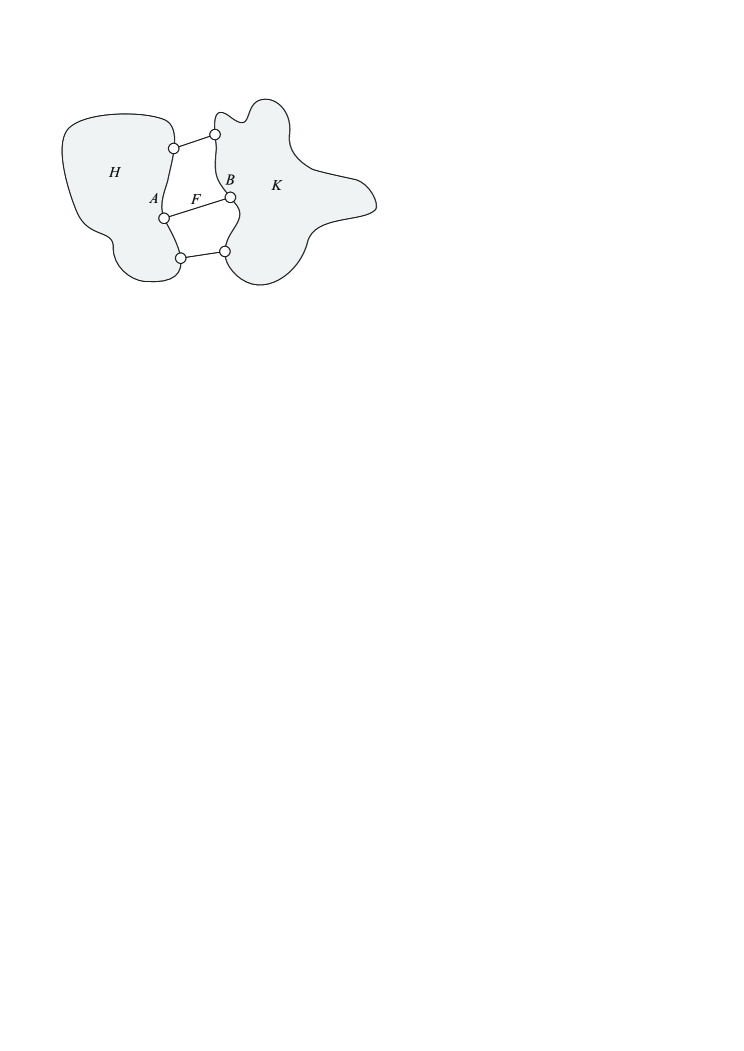
Figure 1: A graph with a matching cut

Theorem 6.

Let $F=\{\{a,b\}\mid a\in A,b\in B\}$ be a minimal cut of a connected graph $G=(V,E)$ such that $F$ is a matching of $G$. The components of $G-F$ are denoted by $H$ and $K$. Assume that $A\subseteq V(H)$ and $B\subseteq V(K)$. We define $H^{\prime}=H\cup(A\cup B,F)$ and $K^{\prime}=K\cup(A\cup B,F)$. Then

$$N(G,x)=N(H^{\prime},x)+N(K^{\prime},x)-2|F|x-1.$$

Figure 1 illustrates the situation of Theorem 6.

Proof.

The open neighborhoods of all vertices of $V(H)$ are the same in $G$ and in $H^{\prime}$. We also have $N_{G}(v)=N_{K^{\prime}}(v)$ for any $v\in V(K)$. This implies

$$\mathcal{N}(G)=\mathcal{N}(H^{\prime})\cup\mathcal{N}(K^{\prime}).$$

Each singleton $\{v\}$ for $v\in A\cup B$ is contained in $\mathcal{N}(H^{\prime})$ and in $\mathcal{N}(K^{\prime})$, which yields $\mathcal{N}(H^{\prime})\cap\mathcal{N}(K^{\prime})=\{\{v\}\mid v\in A\cup B\}\cup\{\emptyset\}$. ∎

2.3 Edge Addition

Let $G=(V,E)$ be a graph, and $u,v\in V$ such that $\{u,v\}\notin E$. Let $G+uv=(V,E\cup\{\{u,v\}\})$ be the graph obtained from $G$ by insertion of the edge $\{u,v\}$. In this case, the neighborhoods of the two vertices $u,v$ have been changed. If there is a path of length 3 between the vertices $u$ and $v$ in $G$, after the edge insertion, a 4-cycle is being formed which causes some difficulties in counting neighborhood sets. In Theorem 7, we suppose that there is no path of length 3 between the vertices $u$ and $v$ to prevent any over-counting and relate the neighborhood polynomial of the new graph after addition the edge $\{u,v\}$ to the neighborhood polynomial of the original graph. In Theorem 8, we investigate the general case.

Theorem 7.

Let $G=(V,E)$ be a graph, $u,v\in V$, and $\{u,v\}\notin E$. Suppose there is no path of length 3 between $u$ and $v$ in $G$. Let $G^{\prime}=(V,E\cup\{\{u,v\}\})$. Then

$$N(G^{\prime},x)=N(G,x)+x((1+x)^{|N_{G}(u)|}-1)+x((1+x)^{|N_{G}(v)|}-1).$$

Proof.

Observe that any vertex subset with a common neighbor in $G$ forms a vertex subset with a common neighbor in $G^{\prime}$. Such vertex subsets are generated by $N(G,x)$. The addition of the edge $\{u,v\}$ to $G$ results in the fact that any non-empty subset of the open neighborhood of $u$ together with $v$ forms a vertex subset with $u$ as the common neighbor in $G^{\prime}$ and the same arguments applies to the open neighborhood of $v$. Such subsets are generated by $x((1+x)^{|N_{G}(u)|}-1)+x((1+x)^{|N_{G}(v)|}-1)$.

Now, assume there is a vertex subset $W$ with a common neighbor in $G^{\prime}$ and suppose it is counted once in $x((1+x)^{|N_{G}(u)|}-1)+x((1+x)^{|N_{G}(v)|}-1)$ and once in $N(G,x)$, and let $y\in W$. This implies that $W$, which is a subset of the open neighborhood of one of the vertices $u$(or $v$) together with $v$ (or $u$) have a common neighbor in $G$. Let $x$ be that common neighbor. The existence of such set results in the existence of a path of length 3 between $u_{1}$ and $u_{2}$ through vertices $x$ and $y$ which contradicts the assumption that there is no path of length 3 between those two vertices in $G$. So there is no vertex subset with a common neighbor in $G^{\prime}$ that is counted twice and this completes the proof. ∎

Theorem 8.

Let $G=(V,E)$ be a graph, $u_{1},u_{2}\in V$, and $(u_{1},u_{2})\notin E$. Suppose $u_{1}$ and $u_{2}$ are not isolated vertices and let $G^{\prime}=(V,E\cup\{\{u_{1},u_{2}\}\})$. Then

$$N(G^{\prime},x)=N(G,x)+x\sum_{\begin{subarray}{c}\emptyset\neq U_{1}\subseteq N_{G}(u_{1})\\ U_{1}\cap N_{G}(u_{2})=\emptyset\end{subarray}}x^{|U_{1}|}+x\sum_{\begin{subarray}{c}\emptyset\neq U_{2}\subseteq N_{G}(u_{2})\\ U_{2}\cap N_{G}(u_{1})=\emptyset\end{subarray}}x^{|U_{2}|}.$$

Proof.

If $X\in\mathcal{N}(G)$ then $X\in\mathcal{N}(G^{\prime})$ and all such vertex subsets are generated by $N(G,x)$. After insertion of the edge $\{u_{1},u_{2}\}$, the vertices in any subset of the open neighborhood of $u_{1}$ together with $u_{2}$ have a common neighbor in $G^{\prime}$ (which is the vertex $u_{1}$), and analogously the vertices in any subset of the open neighborhood of $u_{2}$ together with $u_{1}$ share a neighbor in $G^{\prime}$ (which is the vertex $u_{2}$). Any of such vertex sets adds a term like $xx^{|U|}$ to the neighborhood polynomial of $G^{\prime}$, where $x$ represents $u_{1}$ or $u_{2}$, and $x^{|U|}$ stands for $U$ as a subset of $N_{G}(u_{2})$ or $N_{G}(u_{1})$, respectively. In order to prevent counting a vertex set of this form that already has a common neighbor in $G$ (and therefore being counted in $N(G,x)$) we consider only those subsets of $N_{G}(u_{2})$ or $N_{G}(u_{1})$ which do not have a common neighbor with $u_{1}$ or $u_{2}$ in $G$, respectively. All such vertex subsets are generated by the term

$$x\sum_{\begin{subarray}{c}\emptyset\neq U_{1}\subseteq N_{G}(u_{1})\\ U_{1}\cap N_{G}(u_{2})=\emptyset\end{subarray}}x^{|U_{1}|}+x\sum_{\begin{subarray}{c}\emptyset\neq U_{2}\subseteq N_{G}(u_{2})\\ U_{2}\cap N_{G}(u_{1})=\emptyset\end{subarray}}x^{|U_{2}|},$$

which completes the proof. ∎

2.4 Vertex Attachment

Suppose $G=(V,E)$ is a simple graph and let $U\subseteq V$. Let

$$G_{U\rhd v}=(V\cup\{v\},E\cup\{\{u,v\}\mid u\in U\})$$

be the graph obtained from $G$ by adding a new vertex $v$ to $V$ and attaching $v$ to all vertices of $U$, so the degree of $v$ in $G_{U\rhd v}$ is $|U|$; in this case the set $U$ is called the vertex attachment set. In case of $U=\emptyset$, the graph $G_{U\rhd v}$ is the disjoint union of $G$ and the single vertex $v$, which implies $\mathcal{N}(G_{U\rhd v})=\mathcal{N}(G)$ and therefore $N(G_{U\rhd v},x)=N(G,x)$. In the following theorem, we investigate the neighborhood polynomial of $G_{U\rhd v}$ in case of $U\neq\emptyset$.

Theorem 9.

Let $G=(V,E)$ be a graph and $U\subseteq V$ be a non-empty set. For each vertex subset $W\subseteq U$, we define a monomial $A_{W}$ by

$$A_{W}=\left\{\begin{array}[]{l}x^{|W|}\text{ if }\bigcap_{w\in W}N_{G}(w)=\emptyset,\\ 0\text{ otherwise.}\end{array}\right.$$

Then

$$N(G_{U\rhd v},x)=N(G,x)+\sum_{\begin{subarray}{c}W\subseteq U\\ W\neq\emptyset\end{subarray}}(-1)^{|W|+1}x(1+x)^{|\cap_{w\in W}N_{G}(w)|}+\sum_{\begin{subarray}{c}W\subseteq U\\ W\neq\emptyset\end{subarray}}A_{W}.$$

Proof.

Assume $X\in\mathcal{N}(G_{U\rhd v})$, which implies that the vertices of $X$ have a common neighbor in $G_{U\rhd v}$. Then, we can distinguish the following cases:

1. Assume $v\notin X$ and $v$ is not a common neighbor of the vertices in $X$. In this case $X\in\mathcal{N}(G)$ and all possibilities for the choice of $X$ are counted in $N(G,x)$.

2. Assume $v\notin X$ but $v$ is a common neighbor of the vertices in $X$. Since the only neighbors of $v$ are the vertices in $U$, then we only need to count those subsets of $U$ which do not have a common neighbor in $G$. We do so by

   $$\sum_{\begin{subarray}{c}W\subseteq U\\ W\neq\emptyset\end{subarray}}A_{W},$$

   where

   $$A_{W}=\left\{\begin{array}[]{l}x^{|W|}\text{ if }\bigcap_{w\in W}N_{G}(w)=\emptyset,\\ 0\text{ otherwise.}\end{array}\right.$$

3. Finally assume $v\in X$. In this case, we need to count all vertex subsets of the open neighborhoods of vertices $u\in U$ where each one of those subsets together with $v$ forms a vertex subset with $u$ as their common neighbor in $G_{U\rhd v}$. To exclude double counting subsets of intersections of the neighborhoods of $u$’s, we use the principle of inclusion-exclusion. Such subsets are generated by

   $$\sum_{\begin{subarray}{c}W\subseteq U\\ W\neq\emptyset\end{subarray}}(-1)^{|W|+1}x(1+x)^{|\cap_{w\in W}N_{G}(w)|},$$

   where the factor $x$ accounts for the vertex $v$ itself.

Finally,the arguments in (a), (b), and (c) together prove the theorem. ∎

In the following corollary we rephrase Theorem 9 in a way that the neighborhood polynomial of a graph resulting from vertex removal (instead of vertex attachment) is investigated.

Corollary 10.

Let $G=(V,E)$ be a graph and $v\in V$. Then we have

$$N(G,x)=N(G-v,x)+\sum_{\begin{subarray}{c}U\subseteq N_{G}(v)\\ U\neq\emptyset\end{subarray}}(-1)^{|U|+1}x(1+x)^{|\cap_{u\in U}N_{G-v}(u)|}+\sum_{\begin{subarray}{c}U\subseteq N_{G}(v)\\ U\neq\emptyset\end{subarray}}A_{U},$$

where for $U\subseteq N_{G}(v)$

$$A_{U}=\left\{\begin{array}[]{l}x^{|U|}\text{ if }\bigcap_{u\in U}N_{G-v}(u)=\emptyset,\\ 0\text{ otherwise.}\end{array}\right.$$

3 The Neighborhood Polynomial of $k$-degenerate Graphs

Corollary 10 suggests a recursion for the neighborhood polynomial of a graph based on removing the vertices of the graph one by one. In this section, we introduce $k$-degenerate graphs in which the calculation of the neighborhood polynomial is efficiently possible using the mentioned recursion.

A simple undirected graph $G=(V,E)$ of order $n$ is called $k$-degenerate if every non-empty subgraph of $G$, including $G$ itself, has at least one vertex of degree at most $k$ for $0<k<n$. Suppose $G=(V,E)$ is a $k$-degenerate graph of order $n$. To apply Corollary 10 we need to select a vertex in $G$ to remove. Since $G$ is $k$-degenerate, the existence of a vertex of degree at most $k$ is guaranteed. Suppose $v_{1}$ is a vertex of degree $k$ in $G$, then we remove it and by using Corollary 10, we have

$$N(G,x) =N(G-v_{1},x)+\sum_{\begin{subarray}{c}U\subseteq N_{G}(v_{1})\\ U\neq\emptyset\end{subarray}}(-1)^{|U|+1}x(1+x)^{|\cap_{u\in U}N_{G-v_{1}}(u)|}$$

$$+\sum_{\begin{subarray}{c}U\subseteq N_{G}(v_{1})\\ U\neq\emptyset\end{subarray}}A_{U}.$$

We define $G_{n}:=G$ where $n$ is the number of vertices of $G$. For each $i$, $0<i<n$, let $G_{n-i}$ be the graph obtained from $G_{n-(i-1)}$ after removing a vertex $v_{i}$ of degree at most $k$. The existence of such vertex is guaranteed by $k$-degeneracy of graph $G$. We define for every non-empty $U\subseteq N_{G_{n-(i-1)}}(v_{i})$

$$A_{U}=\left\{\begin{array}[]{l}x^{|U|}\text{ if }\bigcap_{u\in U}N_{G_{n-i}}(u)=\emptyset,\\ 0\text{ otherwise.}\end{array}\right.$$

and for each $i$, $0<i<n$

$$X_{i}=\sum_{U\subseteq N_{G_{n-(i-1)}}(v_{i}),U\neq\emptyset}[(-1)^{|U|+1}x(1+x)^{|\cap_{u\in U}N_{G_{n-i}}(u)|}+A_{U}]$$

Then we have

$$N(G_{n},x) =N(G_{n-1},x)+X_{1}$$

$$=(N(G_{n-2},x)+X_{2})+X_{1}$$

$$\quad\vdots$$

$$=(\cdots((N(G_{1},x)+X_{n-1})+X_{n-2})+\cdots)+X_{1})$$

$$=1+\sum_{i=1}^{n-1}X_{i}$$

where the last equation is a result of the fact that $G_{1}$ is nothing than a single vertex which has neighborhood polynomial $1$.

Clearly, in each step (in other words for each $i$, $0<i<n$), we remove a vertex $v_{i}$ of degree at most $k$ (where its existence is guaranteed due to $k$-degeneracy of $G$) and calculate the term $X_{i}$ that is a sum over all non-empty subsets of $N_{G_{n-(i-1)}}(v_{i})$, but since this set has at most $k$ elements due to the degree of $v_{i}$ in $G_{n-(i-1)}$ the calculation of $N(G,x)$ can be done in polynomial time for any fixed $k$ which yields the following theorem.

Theorem 11.

Let $k$ be a fixed positive integer. The calculation of the neighborhood polynomial can be performed in polynomial-time in the class of $k$-degenerate graphs.

The recursive procedure for the calculation of the neighborhood polynomial becomes for graphs with regular structure especially simple. We give here an example of a $2\times n$-grid graph that can easily be generalized to similar graphs with regular structure.

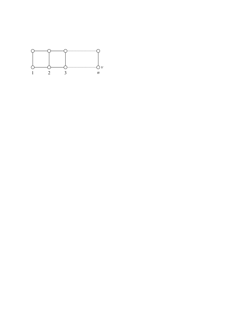
Figure 2: A ladder graph $L_{n}$

Figure 3: A modified ladder graph $M_{n}$

Example 12.

A ladder graph of order $2n$, denoted by $L_{n}$, is the Cartesian product of two path graphs $P_{2}$ and $P_{n}$, see Figure 2. The neighborhood polynomial of $L_{n}$ is

$$N(L_{n},x)=1+4x+2x^{2}+(2n-4)x(1+x)^{2}\quad\text{ for }n\geq 4.$$

To prove this equation we can calculate the neighborhood polynomial of $L_{n}$ by applying Theorem 3, but since $L_{n}$ is $2$-degenerate, we can also apply Corollary 10. To do so, we need to specify a vertex to remove. In the following, we remove a vertex of degree $2$, denoted by $v$ in Figure 2. After removing the vertex $v$, we obtain a modified ladder graph that we denote by $M_{n}$, see Figure 3. The graph $M_{n}$ has exactly one vertex of degree $1$. This is the vertex to be removed in the next step; it is denoted by $v$ in Figure 3.

By Corollary 10, we obtain

$$N(L_{n},x)=N(M_{n},x)+x(1+x)^{2}\quad\text{ for }n\geq 4$$ (3)

and

$$N(M_{n},x)=N(L_{n-1},x)+x(1+x)^{2}\quad\text{ for }n\geq 5.$$ (4)

Substituting $N(M_{n},x)$ in Equation (3) according to Equation (4) yields

$$N(L_{n},x)=N(L_{n-1},x)+2x(1+x)^{2}\quad\text{ for }n\geq 4,$$ (5)

which provides together with the initial value

$$N(L_{2},x)=N(C_{4},x)=1+4x+2x^{2}$$

the above given result.

As any $k$-regular graph is $k$-degenerate, we obtain the following result.

Corollary 13.

Let $k$ be a fixed positive integer. The calculation of the neighborhood polynomial can be performed in polynomial-time in the class of $k$-regular graphs.

As a consequence of Euler’s polyhedron formula, each simple planar graph contains a vertex of degree at most 5. This implies that any simple planar graph is 5-degenerate, which provides the next statement.

Corollary 14.

The neighborhood polynomial of a simple planar graph can be found in polynomial-time.

There is an interesting generalization of planar graphs which was introduced in [Gub96] that belongs to the class of $k$-degenerate graphs, too. An almost planar graph is a non-planar graph $G=(V,E)$ in which for every edge $e\in E$, at least one of the graphs $G-e$ (obtained from $G$ after removing $e$) and $G/e$ (obtained from $G$ by contraction of $e$) is planar. It can be easily shown that every finite almost-planar graph is 6-degenerate, which implies that its neighborhood polynomial can be efficiently calculated.

4 Conclusions and Open Problems

The presented decomposition and reduction methods for the calculation of the neighborhood polynomial work well for graphs of bounded degree or, more generally, for $k$-degenerate graphs. They can easily be extended to derive the neighborhood polynomials of further graphs with regular structure such as grid graphs with additional diagonal edges. The splitting formula for vertex separators also suggests that the neigborhood polynomial should be polynomial-time computable in the class of graphs of bounded treewidth.

A main open problem remains the calculation of the neighborhood polynomial of graphs for which the number of edges is not linearly bounded by its order. Can we find an efficient way to calculate the neighborhood polynomial of graphs of bounded clique-width?

References

- [AAP10] Saieed Akbari, Saeid Alikhani and Yee-hock Peng “Characterization of graphs using domination polynomials” In European Journal of Combinatorics 31.7 Elsevier, 2010, pp. 1714–1724
- [AL00] Jorge Luis Arocha and Bernardo Llano “Mean value for the matching and dominating polynomials” In Discussiones Mathematicae Graph Theory 20, 2000, pp. 57–69
- [BCS09] Andries E Brouwer, P Csorba and A Schrijver “The number of dominating sets of a finite graph is odd” In preprint, 2009
- [BN08] Jason I Brown and Richard J Nowakowski “The neighbourhood polynomial of a graph” In Australasian Journal of Combinatorics 42 Citeseer, 2008, pp. 55–68
- [Dod16] Markus Dod “The Independent Domination Polynomial” In arXiv preprint arXiv:1602.08250, 2016
- [DT12] Klaus Dohmen and Peter Tittmann “Domination reliability” In The Electronic Journal of Combinatorics 19.1, 2012, pp. #P15
- [Gub96] Bradley S Gubser “A characterization of almost-planar graphs” In Combinatorics, Probability and Computing 5.3 Cambridge University Press, 1996, pp. 227–245
- [HT17] Irene Heinrich and Peter Tittmann “Counting Dominating Sets of Graphs” In arXiv preprint arXiv:1701.03453, 2017
- [Kot+12] Tomer Kotek et al. “Recurrence relations and splitting formulas for the domination polynomial” In The Electronic Journal of Combinatorics 19.3, 2012, pp. 47
- [KPT14] Tomer Kotek, James Preen and Peter Tittmann “Subset-sum representations of domination polynomials” In Graphs and Combinatorics 30.3 Springer, 2014, pp. 647–660
- [Lov78] László Lovász “Kneser’s conjecture, chromatic number, and homotopy” In Journal of Combinatorial Theory, Series A 25.3, 1978, pp. 319–324