Model-based free-breathing cardiac MRI reconstruction using deep learned & STORM priors: MoDL-STORM

Abstract: We introduce a model-based reconstruction framework with deep learned (DL) and smoothness regularization on manifolds (STORM) priors to recover free breathing and ungated (FBU) cardiac MRI from highly undersampled measurements. The DL priors enable us to exploit the local correlations, while the STORM prior enables us to make use of the extensive non-local similarities that are subject dependent. We introduce a novel model-based formulation that allows the seamless integration of deep learning methods with available prior information, which current deep learning algorithms are not capable of. The experimental results demonstrate the preliminary potential of this work in accelerating FBU cardiac MRI.
Index Terms—  Free breathing cardiac MRI, model-based, inverse problems, deep CNNs

1 Introduction

The acquisition of cardiac MRI data is often challenging due to the slow nature of MR acquisition. The current practice is to integrate the information from multiple cardiac cycles, while the subject is holding the breath. Unfortunately, this approach is not practical for several populations, including pediatric and obese subjects. Several self-gated strategies [1], which identify the respiratory and cardiac phases to bin the data and reconstruct it, have been introduced to enable free breathing and ungated (FBU) cardiac MRI. The recently introduced, smoothness regularization on manifolds (STORM) prior in [2] follows an implicit approach of combining the data from images in a data-set with similar cardiac respiratory phases. All of the current gating based methods require relatively long ($\approx$ 1 minute) acquisitions to ensure that sufficient Fourier or k-space information is available for the recovery.

Several researchers have recently proposed convolutional neural network (CNN) architectures for image recovery [3, 4, 5]. A large majority of these schemes retrained existing architectures (e.g., UNET or ResNet) to recover images from measured data. The above strategies rely on a single framework to invert the forward model (of the inverse problem) and to exploit the extensive redundancy in the images. Unfortunately, this approach cannot be used directly in our setting. Specifically, the direct recovery of the data-set using CNN priors alone is challenging due to the high acceleration (undersampling) needed ($\approx$50 fold acceleration); the use of additional k-space information from similar cardiac/respiratory phases is required to make the problem well posed. Here, high acceleration means reduced scan time which is achieved with undersampling. None of the current CNN image recovery schemes are designed to exploit such complementary prior information, especially when the prior depends heavily on cardiac and respiratory patterns of the specific subject. Another challenge is the need for large networks with many parameter to learn the complex inverse model, which requires extensive amounts of training data and significant computational power. More importantly, the dependence of the trained network on the acquisition model makes it difficult to reuse a model designed for a specific undersampling pattern to another one. This poses a challenge in the dynamic imaging setting since the sampling patterns vary from frame to frame.

The main focus of this work is to introduce a model based framework, which merges the power of deep learning with model-based image recovery to reduce the scan time in FBU cardiac MRI. Specifically, we use a CNN based plug-and-play prior. This approach enables easy integration with the STORM regularization prior, which additionally exploits the subject dependent non-local redundancies in the data. Since we make use of the available forward model, a low-complexity network with a significantly lower number of trainable parameters is sufficient for good recovery, compared to black-box (CNN alone) image recovery strategies; this translates to faster training and requires less training data. More importantly, the network is decoupled from the specifics of the acquisition scheme and is only designed to exploit the redundancies in the image data. This allows us to use the same network to recover different frames in the data-set, each acquired using a different sampling pattern. The resulting framework can be viewed as a iterative network, where the basic building block is a combination of a data-consistency term and a CNN; unrolling the iterative network yields a network. Since it is impossible to acquire fully sampled FBU data, we validate the framework using retrospective samples of STORM [2] reconstructed data, recovered from 1000 frames (1 minute of acquisition). In this work, we aim to significantly shorten the acquisition time to 12-18 secs (200-300 frames) by additionally capitalizing on the CNN priors.

The main difference between the proposed scheme and current unrolled CNN methods [6, 7] is the reuse of the CNN weights at each iteration; in addition to reducing the trainable parameters, the weight reuse strategy yields a structure that is consistent with the model-based framework, facilitating its easy use with other regularization terms. In addition, the use of the CNN as a plug and play prior rather than a custom designed variational model [7] allows us to capitalize upon the well-established software engineering frameworks such as Tensorflow and Theano.

2 Proposed method

We note that the STORM prior does not exploit the local similarities, such as smooth nature of the images or the similarity of an image with its immediate temporal neighbors. In contrast, the 3-D CNN architecture is ideally suited to exploit the local similarities in the dynamic data-set. To capitalize on the complementary benefits of both methods, we introduce the model based reconstruction scheme to recover the free breathing dynamic data-set $\mathbf{X}$

$$\mathcal{C}({\mathbf{X}}) = \underbrace{\|\mathcal{A}({\mathbf{X}})-{\mathbf{B}}\|_{2}^{2}}_{\mbox{data consistency}}~{}+~{}\lambda_{1}\underbrace{\|\mathcal{N}_{{\mathbf{w}}}({\mathbf{X}})\|^{2}}_{\mbox{CNN prior}}$$ (1)

$$+\qquad\lambda_{2}\underbrace{{\rm tr}\left(\mathbf{X}^{T}\mathbf{L}\mathbf{X}\right)}_{\mbox{STORM prior}}.$$

Here, $\mathcal{A}$ is the Fourier measurement operator. The second and third terms are the regularization terms, which exploit the redundancy in the images. $\mathcal{N}_{\rm w}$ is a learned CNN estimator of noise and alias patterns, which depends on the learned network parameters $\mathbf{w}$. Specifically, $\|\mathcal{N}_{\mathbf{w}}(\mathbf{x})\|^{2}$ is high when $\mathbf{x}$ is contaminated with noise and alias patterns; its use as a prior will encourage solutions that are minimally contaminated by noise and alias patterns. Since $\mathcal{N}_{\mathbf{w}}(\mathbf{X})$ is an estimate of the noise and alias terms, one may obtain the denoised estimate as

$$\mathcal{D}_{\mathbf{w}}(\mathbf{X})=\left(\mathcal{I}-\mathcal{N}_{\rm w}\right)(\mathbf{X})=\mathbf{X}-\mathcal{N}_{\mathbf{w}}(\mathbf{X}).$$ (2)

This reinterpretation shows that $\mathcal{D}_{\mathbf{w}}$ can be viewed as a denoising residual learning network. When $\mathcal{D}_{\mathbf{w}}$ is a denoiser, $\mathcal{N}_{\mathbf{w}}(\mathbf{X})=\mathbf{X}-\mathcal{D}_{\mathbf{w}}(\mathbf{X})$ is the residual in $\mathbf{X}$. With this interpretation, the CNN prior can be expressed as $\|\mathbf{X}-\mathcal{D}_{\mathbf{w}}(\mathbf{X})\|^{2}$.

The third term in (1) is the STORM prior, which exploits the similarities between image frames with the same cardiac and respiratory phase; $\rm tr$ denotes the trace operator. Here, $\mathbf{L}=\mathbf{D}-\mathbf{W}$ is the graph Laplacian matrix, estimated from the k-space navigators [2]. $\mathbf{W}$ is a weight matrix, whose entries are indicative of the similarities between image frames. Specifically, ${\mathbf{W}}_{(i,j)}$ is high if ${\mathbf{x}}_{i}$ and ${\mathbf{x}}_{j}$ have similar cardiac/respiratory phase. $\mathbf{D}$ is a diagonal matrix, whose diagonal entries are given by $\mathbf{D}_{(i,i)}=\sum_{j}\mathbf{W}_{(i,j)}$.

2.1 Implementation

(a) Proposed model based framework

(b) Unfolded network

Fig. 1: Illustration of the MoDL-STORM architecture. (a) indicates the iterative structure denoted by (5)-(8). Here, $\mathcal{D}_{w}$ denotes the denoising residual network, shown with the yellow box. This residual learning is performed using an out of the box CNN approach. (b) Once the number of iterations $N$ is fixed, the network can be unrolled to obtain a non-iterative unrolled deep learning model, which relies on weight sharing.

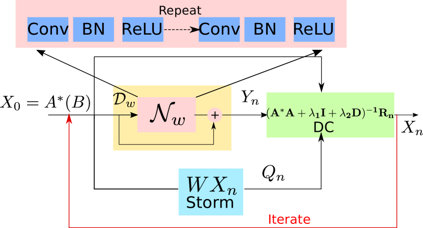
We re-express the STORM prior in (1) using an auxiliary variable ${\mathbf{X}}={\mathbf{Z}}$:

$$2{\rm tr}(\mathbf{X}^{T}\mathbf{L}\mathbf{X})={\rm tr}(\mathbf{X}^{T}\mathbf{D}\mathbf{X})+{\rm tr}(\mathbf{Z}^{T}\mathbf{D}\mathbf{Z})-2{\rm tr}(\mathbf{X}^{T}\mathbf{W}\mathbf{Z})$$ (3)

This alternate expression allow us to rewrite (1) using two auxiliary variables ${\mathbf{Y}}=\mathcal{D}_{\mathbf{w}}(\mathbf{X})$ and ${\mathbf{Z}}={\mathbf{X}}$:

$$\mathcal{C} = \|\mathcal{A}({\mathbf{X}})-{\mathbf{B}}\|_{2}^{2}+\lambda_{1}\|{\mathbf{X}}-{\mathbf{Y}}\|^{2}+$$

$$\qquad\lambda_{2}\left({\rm tr}(\mathbf{X}^{T}\mathbf{D}\mathbf{X})+{\rm tr}(\mathbf{Z}^{T}\mathbf{D}\mathbf{Z})-2{\rm tr}(\mathbf{X}^{T}\mathbf{W}\mathbf{Z})\right)$$

We propose to use an update strategy, where we assume ${\mathbf{Z}}$ and ${\mathbf{Y}}$ to be fixed and minimize the expression with respect to ${\mathbf{X}}$. The variables ${\mathbf{Z}}$ and ${\mathbf{Y}}$ are then updated based on the previous iterate. The minimization of $\mathcal{C}$ w.r.t ${\mathbf{X}}$ yields

$$\nabla C=\mathcal{A}^{*}(\mathcal{A}({\mathbf{X}})-{\mathbf{B}})+\lambda_{1}({\mathbf{X}}-{\mathbf{Y}})+\lambda_{2}\left({\mathbf{D}}{\mathbf{X}}-{\mathbf{W}}{\mathbf{Z}}\right)=0$$ (4)

where $\mathcal{A}^{*}$ is the adjoint of the operator $\mathcal{A}$. This normal equation which gives the update rules

$${\mathbf{Y}}_{n} = \mathcal{D}_{{\mathbf{w}}}({\mathbf{X}}_{n})$$ (5)

$${\mathbf{Q}}_{n} = {\mathbf{W}}{\mathbf{Z}}_{n}={\mathbf{W}}{\mathbf{X}}_{n}$$ (6)

$${\mathbf{R}}_{n} = \left(\mathcal{A}^{*}({\mathbf{B}})+\lambda_{1}{\mathbf{Y}}_{n}+\lambda_{2}{\mathbf{Q}}_{n}\right)$$ (7)

$$\mathbf{X}_{n+1} = (\mathcal{A}^{*}\mathcal{A}+\lambda_{1}{\mathbf{I}}+\lambda_{2}{\mathbf{D}})^{-1}\mathbf{R}_{n}$$ (8)

Note that since we rely on 2-D sampling on a frame by frame basis and because ${\mathbf{D}}$ is a diagonal matrix, the matrix $(\mathcal{A}^{*}\mathcal{A}+\lambda_{1}{\mathbf{I}}+\lambda_{2}{\mathbf{D}})$ is separable; it can be solved analytically on a frame by frame basis in the Fourier domain; we term this operation as the data consistency (DC) step. Specifically, the update rule for the $i^{\rm th}$ frame is given by

$${\mathbf{x}}_{n+1}^{(i)}=\left[{\mathbf{A}}_{i}^{H}{\mathbf{A}}_{i}+\left(\lambda_{1}+\lambda_{2}d_{i}\right){\mathbf{I}}\right]^{-1}({\mathbf{A}}_{i}^{H}{\mathbf{B}}+\lambda_{1}{\mathbf{y}}_{n}^{(i)}+\lambda_{2}{\mathbf{q}}_{n}^{(i)})$$ (9)

where ${\mathbf{A}}_{i}={\mathbf{S}}_{i}{\mathbf{F}}$ and $d_{i}={\mathbf{D}}_{i,i}$. Here, ${\mathbf{S}}_{i}$ is the sampling pattern in the $i^{\rm th}$ frame and ${\mathbf{F}}$ is the 2D Fourier transform. ${\mathbf{y}}_{n}^{(i)}$ is the $i^{\rm th}$ frame of ${\mathbf{Y}}_{n}$, which is the CNN denoised version of the $n^{\rm th}$ iterate ${\mathbf{X}}_{n}$. Likewise, ${\mathbf{q}}_{n}^{(i)}$ is the $i^{\rm th}$ frame of ${\mathbf{Q}}_{n}$, which is the STORM denoised version of ${\mathbf{X}}_{n}$, with the exception that each column of ${\mathbf{Q}}_{n}$ is scaled by $d_{i}$. This update rule shows that the framework is very similar to [8], where the power of existing denoising algorithms are capitalized as plug and play priors in a model based regularization framework. The algorithm alternates between signal recovery and denoising steps.

This iterative algorithm is illustrated in Fig. 1.(a), where we initialize the algorithm with ${\mathbf{X}}_{0}=\mathcal{A}^{*}(\mathbf{B})$. The STORM and CNN denoised signals ${\mathbf{Q}}$ and ${\mathbf{Y}}$ are then fed into the DC block specified by (8). Once the number of iterations are fixed, we can obtain the unrolled network, which is illustrated in Fig. 1.(b). We observe that 5-8 iterations of the network is often sufficient for good recovery.

2.2 Training phase

We propose to train the unrolled CNN shown in Fig. 1.b. Specifically, we present the network with exemplar data consisting of undersampled data ${\mathbf{B}}$ as the input and their reconstructions as the desired output. The CNN parameters are learned to minimize the reconstruction error, in the mean square sense. Unfortunately, it is difficult to present the network with a full data-set ($\approx$ 200 frames) in the training mode. Specifically, the feature maps for each layer need to be stored for the evaluation of gradients by back-propagation, which is difficult on GPU devices with limited onboard memory.

Note that both the CNN and the data-consistency layer perform local operations. If the STORM prior was not present, one could pass smaller subsets of input and output (e.g. 20-30 frames) data in multiple batches for training. In contrast, the STORM prior uses non-local or global information from the entire data-set. Specifically, for the evaluation of the $i^{\rm th}$ frame of ${\mathbf{Q}}_{n}$, specified by ${\mathbf{q}}_{n}^{(i)}$, we require the entire data-set. We hence propose a lagged approach, where ${\mathbf{Q}}_{n}$ is updated less frequently than the other parameters. Specifically, we use an outer loop to update ${\mathbf{Q}}_{n}$, while the trainable parameters of the CNN ${\mathbf{w}}$ and the regularization parameters $\lambda_{1}$ and $\lambda_{2}$ are updated assuming ${\mathbf{Q}}_{n}$ to be fixed. We feed in batches of 20-30 frames of training data. The network during this training mode is illustrated in Fig. 2. After one such training, we run the model on the entire data-set to determine the ${\mathbf{X}}_{n};n=0,..,N-1$ for all 204 frames. The variables ${\mathbf{Q}}_{n}$ are updated using (6), which are then used in the next training.

Result: ${\mathbf{X}}_{n}$

Define: $\mathcal{D}_{{\mathbf{w}}},\mathcal{A}.$ Inputs: ${\mathbf{B}},{\mathbf{X}}_{0}=\mathcal{A}^{*}(B)$;

while $j<$ NOuter, do

       ${\mathbf{Q}}_{n}={\mathbf{W}}{\mathbf{X}}_{n};\forall n\in[0,N]$;

       Train model in Fig. 2 with fixed ${\mathbf{Q}}_{n}$ $j=j+1$;

end while

Algorithm 1 Pseudo-code for our iterative algorithm. The variables ${\mathbf{Q}}_{n};n=0,..,N$ are not updated while the network is trained using backpropagation. This strategy allows us to keep the memory demand of the algorithm limited, allowing us to train the network on current GPU devices.

Fig. 2: Modified network used in training illustrated in Algorithm 1. The main difference between the unrolled network in Fig.1.(b) is that the variables ${\mathbf{Q}}_{n};n=0,..,N$ are assumed to be fixed. These variables are estimated in the outer loop as shown in Algorithm 1.

3 Experimental details

The raw data data was acquired using a golden angle FLASH sequence with k-space navigators on a Siemens Aera scanner from congenital heart patients with FOV=300 mm, slice thickness=5 mm, radial views=10000, base resolution=256, TR/TE=4.68/2.1 ms, resulting in an acquisition time of $\approx 50$ s, was binned to frames with 12 lines/frame and reconstructed using the STORM algorithm using [2], where 4 channel k-space data obtained by PCA combining the data from 24 channels were used. Note that the direct acquisition and reconstruction of similar data-sets are impossible. Sub-segments of this data, each consisting of 204 frames, were used to train the proposed scheme; note that our objective is to reduce the acquisition window to around 15-20 seconds. The recovered data was retrospectively undersampled to 17 lines/frame, consisting of 4 navigator and 13 golden angle lines. The navigator lines were only used for the Laplacian estimation and not used for final reconstruction. We assumed single channel acquisition for simplicity.

We implemented the CNN network $\mathcal{D}_{\mathbf{w}}$ in TensorFlow with a 3D kernel size of $3\times 3$, five layers, and 64 filters per layer. We considered the number of iterations of the network to be $N=8$. Each layer was a cascade of 3D convolution, batch normalization and a ReLU activation. Since the memory demands restricted the training using all 204 frames in the data-set, we split the data into batches of 17 frames each, extracted from the original data-set. Note that the sampling pattern for each frame used in training is different; since the model based framework uses the numerical model for the acquisition scheme, it can account for this variability without requiring a very deep network with several trainable parameters. As discussed previously and illustrated in Algorithm 1, we pre-compute the variables ${\mathbf{Q}}_{n};n=1,..,N$ and assume them to be fixed during the deep learning training procedure. We restricted the cost function to only include comparisons with the middle frames in the output to reduce boundary issues; the mean square error cost function was used to perform the optimization. We relied on ADAM optimizer with its default hyperparameters to train the network weights as well as the regularizers, $\lambda_{1},\lambda_{2}$. We used 200 epochs of network training for each outer loop. The training time for 200 epochs is around 2.5 hours; the total time taken for $NOuter=4$ is $\approx 11$ hours on a NVDIA P100 GPU processor.

Once the training is complete, the reconstruction follows the unfolded network in Fig. 1.b. Specifically, the entire undersampled single channel k-space data corresponding to the 204 frame data-set is fed to the trained network. Since the network just requires eight repetitions and the basic steps involve convolutions and fast Fourier transforms, hence the reconstructions are fast. Testing time for 204 frames with $N=8$ repetitions was 38 seconds.

4 Results & Conclusion

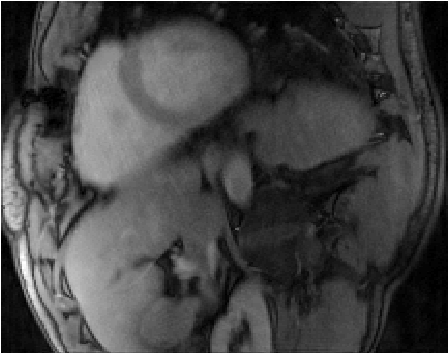
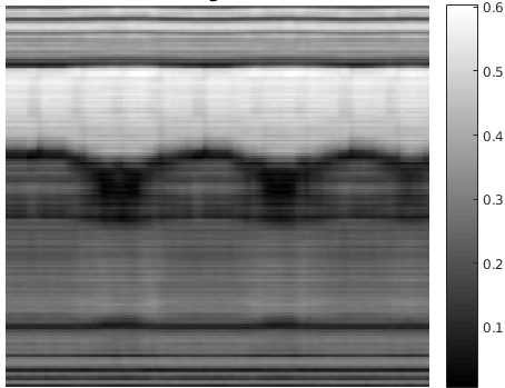
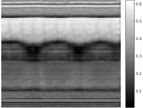
Fig 3 shows the reconstruction results with corresponding to 17 lines/frame) using single channel data. This data is used as the ground truth for the reconstruction. A similar STORM reconstructed data-set from another patient was used for training. These comparisons show that the combination of deep learning and STORM priors yield reconstructions that are comparable in quality to the ground truth.

(a) Ground truth

(b) Gridding: SNR=6.8 dB

(c) MoDL:SNR=13.0 dB

(d) MoDL-STORM: SNR=23.1dB

(e) Ground truth

(f) MoDL-STORM

Fig. 3: Reconstruction results at 16 fold acceleration. The ground truth data, recovered from 50 second (1000 frames) acquisition using STORM is shown in (a). The data from a subset of 204 frames is retrospectively downsampled assuming single channel acquisition and tested using different algorithm. The zero-filled IFFT reconstruction is shown in (b). A reconstructed frame using a network similar to ours without STORM priors (only CNN) is shown in (c). Note that the exploitation of the local similarities enabled by CNN alone is insufficient to provide good reconstructions at 16 fold acceleration. In contrast, the combination of deep learning and STORM priors yield reconstructions that are comparable in quality to the ground truth. The temporal profiles of the ground truth and MoDL-STORM reconstructions are shown in (e) and (f), respectively

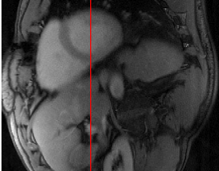
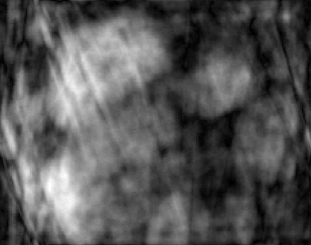
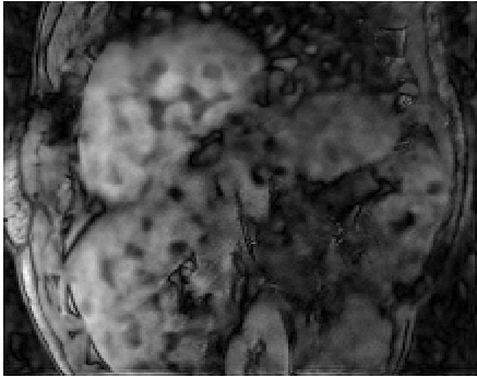
We introduced model based dynamic MR reconstruction for free breathing and ungated cardiac MRI. The proposed framework enables the seamless integration of deep learned architectures with other regularization terms. It additionally exploits the prior information that is subject dependent (e.g. due to respiratory variations and cardiac rate). The preliminary study in this paper shows that the proposed framework enables us to significantly reduce the acquisition time in free breathing approaches. Our future work will focus on demonstrating the power of the framework on prospectively acquired data. We also plan to capitalize on the multichannel data, which is not exploited in this work for simplicity.

References

- [1] L. Feng, R. Grimm, K. T. Block, H. Chandarana, S. Kim, J. Xu, L. Axel, D. K. Sodickson, and R. Otazo, “Golden-angle radial sparse parallel mri: Combination of compressed sensing, parallel imaging, and golden-angle radial sampling for fast and flexible dynamic volumetric mri,” Magnetic resonance in medicine, vol. 72, no. 3, pp. 707–717, 2014.
- [2] S. Poddar and M. Jacob, “Dynamic mri using smoothness regularization on manifolds (storm),” IEEE transactions on medical imaging, vol. 35, no. 4, pp. 1106–1115, 2016.
- [3] S. Diamond, V. Sitzmann, F. Heide, and G. Wetzstein, “Unrolled Optimization with Deep Priors,” in arXiv:1705.08041, 2017, pp. 1–11. [Online]. Available: http://arxiv.org/abs/1705.08041
- [4] K. H. Jin, M. T. McCann, E. Froustey, and M. Unser, “Deep Convolutional Neural Network for Inverse Problems in Imaging,” IEEE Transactions on Image Processing, vol. 29, pp. 4509–4522, 2017.
- [5] D. Lee, J. Yoo, and J. C. Ye, “Deep Residual Learning for Compressed Sensing MRI,” in IEEE International Symposium on Biomedical Imaging, 2017, pp. 15–18.
- [6] J. Schlemper, J. Caballero, J. V. Hajnal, A. Price, and D. Rueckert, “A Deep Cascade of Convolutional Neural Networks for MR Image Reconstruction,” in Information Processing in Medical Imaging, 2017, pp. 647–658.
- [7] K. Hammernik, T. Klatzer, E. Kobler, M. P. Recht, D. K. Sodickson, T. Pock, and F. Knoll, “Learning a Variational Network for Reconstruction of Accelerated MRI Data,” in arXiv:1704.00447v1. Graz University of Technology, Austria, 2017, pp. 1–29.
- [8] S. H. Chan, X. Wang, and O. A. Elgendy, “Plug-and-Play ADMM for Image Restoration: Fixed Point Convergence and Applications,” IEEE Transactions on Computational Imaging, vol. 3, no. 1, pp. 84–98, 2017. [Online]. Available: http://arxiv.org/abs/1605.01710