Verification of Uncertain POMDPs Using Barrier Certificates
Abstract
We consider a class of partially observable Markov decision processes (POMDPs) with uncertain transition and/or observation probabilities. The uncertainty takes the form of probability intervals. Such uncertain POMDPs can be used, for example, to model autonomous agents with sensors with limited accuracy, or undergoing a sudden component failure, or structural damage [1]. Given an uncertain POMDP representation of the autonomous agent, our goal is to propose a method for checking whether the system will satisfy an optimal performance, while not violating a safety requirement (e.g. fuel level, velocity, and etc.). To this end, we cast the POMDP problem into a switched system scenario. We then take advantage of this switched system characterization and propose a method based on barrier certificates for optimality and/or safety verification. We then show that the verification task can be carried out computationally by sum-of-squares programming. We illustrate the efficacy of our method by applying it to a Mars rover exploration example.
I INTRODUCTION
A popular formal model for planning subject to stochastic behavior are Markov decision processes (MDPs) [2], where an agent chooses to perform an action under full knowledge of the environment it is operating in. The outcome of the action is a probability distribution over the system states. Many applications, however, allow only partial observability of the current system state [3, 4, 5]. Partially observable Markov decision processes (POMDPs) extend MDPs to account for such partial information [6]. Upon certain observations, the agent infers the likelihood of the system being in a certain state, called the belief state. The belief state together with an update function form a (typically uncountably infinite) MDP, referred to as the belief MDP [7, 8, 9, 10, 11].
Most formulations assume the the transition probability function and the observation function for MDPs and POMDPs are explicitly given. Unforeseeable events such as (unpredictable) structural damage to a system [12] or an imprecise sensor model [13], however, necessitate a more robust formalism. So-called uncertain MDPs incorporate uncertainty-sets of probabilities, for instance, for models that are empirically determined. Similar extensions exist for uncertain POMDPs [14, 15, 16].
Here, we aim to address current challenges for the area of artificial intelligence, referred to as robust decision-making and safe exploration [17, 18, 19, 20]. Concretely, the problem is to provide a policy for an (autonomous) agent that ensures certain desired behavior by robustly accounting for any uncertainty and partial observability that may occur in the system [21]. The policy should be optimal with respect to some performance measure and additionally ensure safe navigation through the environment.
However, already for mere POMDPs (without uncertainties in the probabilities), such policies are computed by assessing the entire belief MDP, rendering the problem undecidable [22]. Several promising approximate point-based methods via finite abstraction of the belief space are proposed in the literature [23, 24, 25]. Nonetheless, these techniques do not provide a guarantee for safety or optimality. That is, it is not clear whether the probability of satisfying the safety/optimality requirement is an upper-bound or a lower-bound for a given POMDP. Establishing guaranteed performance is of fundamental importance in safety-critical applications, e.g. aircraft collision avoidance [26] and Mars rovers [27].
In this paper, we borrow a notion from control theory to provide guarantees for optimality and safety of uncertain POMDPs, without the need for finite abstraction. We first demonstrate that POMDP analysis problems can be represented as analyzing the solutions of a special discrete-time switched systems [28]. In particular, POMDPs with uncertain transition and/or observation probabilities belonging to intervals can be characterized as a class of switched systems with parametric uncertainty. Based on this switched system representation, we verify the safety and/or optimality requirements of a given POMDP using barrier certificates [29] (see our preliminary results with application to privacy verification of POMDPs [30]). We show that if there exist a barrier certificate satisfying a set of inequalities along the belief update equation of the POMDP, the safety/optimality property is guaranteed to hold. These conditions can be computationally implemented as a set of sum-of-squares programs (see Appendix -A for a brief introduction). We elucidate the proposed method by applying it to an uncertain POMDP model for a Mars rover with uncertain sensor accuracy sampling rocks on the Mars terrain.
The rest of the paper is organized as follows. In the subsequent section, we define the notations used in this paper and review some preliminary definitions. In Section III, we describe the class of uncertainties and the properties that we are interested in. In Section IV, we propose a switched system representation for POMDPs, and present conditions based on barrier certificates for checking optimality and/or safety. In Section V, we apply the proposed method to verify the performance of an uncertain POMDP model of a Mars rover sampling rocks. Finally, in Section VI, we conclude the paper and give directions for future research.
II Preliminaries
Notation: The notations employed in this paper are relatively straightforward. denotes the set . denotes the set of integers and for implies the set . accounts for the set of polynomial functions with real coefficients in , and is the subset of polynomials with a sum-of-squares decomposition; i.e, if and only if there are such that . For a finite set , denotes the number of elements in .
II-A Partially Observable Markov Decision Processes
Markov decision processes (MDPs) [2] are decision-making modeling framework, in which the actions have stochastic outcomes. An MDP has the following components:
-
•
is a finite set of states with indices .
-
•
defines the distribution of the initial states, i.e., denotes the probability of starting at .
-
•
is a finite set of actions.
-
•
is the probabilistic transition function, where
(1)
POMDPs provide a more general mathematical framework to consider not only the stochastic outcomes of actions, but also the imperfect state observations [31]. Formally, a POMDP is defined with the following components:
-
•
are the same as the definition of an MDP.
-
•
is the set of all possible observations representing outputs of a discrete sensor. Usually is an incomplete projection of the world state , contaminated by sensor noise.
-
•
is the observation probability transition function (sensor model), where
(2)
Since the states are not directly accessible in a POMDP, decision making requires the history of observations. Therefore, we need to define the notion of a belief or the posterior as sufficient statistics for the history [32]. Given a POMDP, the belief at is defined as and denotes the probability of system being in state at time . At time , when action is observed, the belief update can be obtained by a Bayesian filter as
| (3) |
where the beliefs belong to the belief unit simplex
A policy in a POMDP setting is then a mapping , i.e., a mapping from the continuous beliefs space into the discrete and finite action space.
III Problem Formulation
We represent the uncertainty in the autonomous agent’s dynamics as a POMDP with uncertain transition and/or observation probabilities. The class of uncertainties we study belong to an interval [33]. Let denote the set of triplets corresponding to the uncertain transition probabilities. Similarly, let denote the set of triplets corresponding to the uncertain observation probabilities. We consider the class of POMDPs with the following interval transition and/or observation probabilities
| (4a) | |||
| (4b) |
where the constants for all and for all .
In the sequel, we focus on the case of uncertain transition probabilities, but the extension to the case of uncertain observation transition probabilities is straightforward and follows the same lines.
III-A Safety and Optimality
For typical POMDP problems, we are often interested in assessing both optimal and safe behavior. In the following, we define the formal notions of optimality and safety we consider here.
We define safety as the probability of reaching a set of unsafe states being less than a given constant. To this end, we use the belief states. Formally, we are interested in solving the following problem.
Problem 1
Given an uncertain POMDP with interval probabilities as described in (4), a point future in time , a set of unsafe states , and a safety requirement constant , check whether
| (5) |
where . In particular, can be an affine function.
In addition to safety, we are interested in checking whether an optimality criterion is satisfied.
Problem 2
Given an uncertain POMDP with interval probabilities as described in (4), the reward function , in which denotes the reward of taking action while being at state , a point future in time , and a optimality requirement , check whether
| (6) |
where .
IV Main Results
Checking whether (5) and (6) hold by solving the POMDP directly is a PSPACE-hard problem [22], not to mention the difficulties arising from uncertain transition probabilities. In this section, we first demonstrate that POMDPs can be represented as discrete-time switched systems. Then, we borrow a notion from control theory to check the safety and/or optimality requirements of a given POMDP with a guarantee or a certificate.
IV-A Treating POMDPs as Switched Systems
The belief update equation (II-A) is a discrete-time switched system, where the actions define the switching modes. Formally, the belief dynamics (II-A) can be described as
| (7) |
where denote the belief vector belonging to the belief unit simplex and representing the set of initial beliefs (prior). In (8), denote the actions that can be interpreted as the switching modes, are the observations representing inputs, and denote the discrete time instances. The vector fields with are described as the vectors with rows
where denotes the th row of . If the transition probabilities are uncertain, i.e., they belong to some given set, the system can be represented as an uncertain discrete-time switched system
| (8) |
where is a set of uncertain parameters and represents the uncertain transition probability intervals (4). That is,
and
| (9) |
In this study, we consider two classes of problems in POMDP verification:
-
1.
No policy is given: This case corresponds to analyzing (8) under arbitrary switching with switching modes given by .
-
2.
A policy is given: This corresponds to to analyzing (8) under state-dependent switching. Indeed, the policy determines regions in the belief space where each mode (action) is active.
Both cases of switched systems with arbitrary switching and state-dependent switching are well-known in the systems and controls literature [28]. The next example illustrates the proposed switched system representation for POMDPs with a given policy.
Example 1
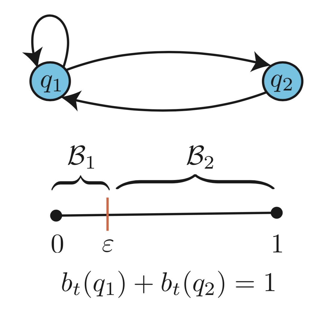
IV-B Verification Using Barrier Certificates
In the following, we show how we can use barrier certificates to verify properties of the switched systems induced by POMDPS.
Theorem 1
Consider the belief update equation (8) and the uncertain transition probabilities (9). Given a set of initial beliefs , an unsafe set as given in (12) (), and a constant , if there exists a function called the barrier certificate such that
| (13) |
| (14) |
and
| (15) |
then there exist no solution of the belief update equation (8) such that , and for all and all .
Proof:
The proof is carried out by contradiction. Assume at time instance there exist a solution to (8) such that and . From inequality (15), we have
for all , all actions , and . Hence, for all . Furthermore, inequality (14) implies that
for all . Since the choice of can be arbitrary, this is a contradiction because it implies that . Therefore, there exist no solution of (8) such that and for any sequence of actions and uncertain probabilities belonging to . Therefore, the safety requirement is satisfied. ∎
The above theorem provides conditions under which the POMDP is guaranteed to be safe. The next result brings forward a set of conditions, which verifies whether the optimality criterion (6) is satisfied.
Corollary 1
Consider the belief update equation (8), the uncertain probabilities (9) and the optimality criterion as given by (6). Let satisfying
| (16) |
Given a set of initial beliefs , an unsafe set
| (17) |
and a constant , if there exists a function such that (13)-(15) are satisfied with instead of , then for all the optimality criterion (6) holds.
Proof:
The proof is straightforward and an application of Theorem 1. If conditions (13)-(15) are satisfied with instead of , based on Theorem 1, we conclude that there exist no solution of the belief update equation (8) such that , and for all and all . Therefore, we have
Summing up both sides of the above equation from to yields
Then, from (16), we conclude that . ∎
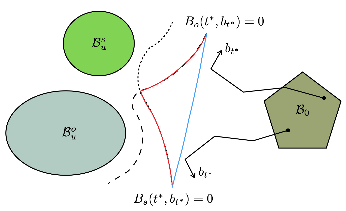
The technique used in Corollary 1 is analogous to the one used in [34, 35] for bounding (time-averaged) functional outputs of systems described by partial differential equations. The method proposed here, however, can be used for a large class of discrete time systems and the belief update equation is a special case that is of our interest.
In practice, it is often desirable to make sure a design is both optimal and safe. The problem can be described by checking whether the solutions of the belief update switched dynamics (8) enter the following set
To this end, we can adopt either of the following approaches (see Figure 2). Both of these approaches are based on the construction of non-smooth barrier certificates. The first one, proposed in [36], suggests finding the barrier certificate for and separately or in parallel. The barrier certificate for the set is then the maximum of the two certificates, i.e., , where is the barrier certificate for checking safety and is the barrier certificate for checking optimality. The second method proposed by the authors in [37, 38] suggests searching for a barrier certificate composed of the convex hull of the and . In this paper, we adopt the latter method.
IV-C Computational Method based on
Sum-of-Squares Programming
The belief update equation (II-A) is a rational function in the belief states ,
| (18) |
The uncertain probabilities are parameters that belong to the set (9). Moreover, the unsafe set (12) and the uncertainty set (9) are semi-algebraic sets, since they can be described by polynomial inequalities. We further assume the set of initial beliefs is also given by a semi-algebraic set as follows
| (19) |
and as in (5).
At this stage, we are ready to present conditions based on sum-of-squares programs to verify safety of a given uncertain POMDP.
Corollary 2
Proof:
Sum-of-squares conditions (20) and (21) are a direct consequence of applying Propositions 1 and 2 in Appendix A to verify conditions (13) and (14), respectively. Furthermore, condition (15) for system (18) can be re-written as
Since is a semi-algebraic set, we use Propositions 1 and 2 in Appendix A to obtain
for , . Given that is a positive polynomial of degree one, we can relax the above inequality into a sum-of-squares condition given by
| (23) |
Hence, if (22) holds, then (15) is satisfied as well. From Theorem 1, we infer that there is no at time such that and . Equivalently, the safety requirement is satisfied at time . That is, . ∎
Checking whether optimality holds can also be cast into sum-of-squares programs. To this end, we assume the reward function is a polynomial (or can be approximated by a polynomial111This assumption is realistic, since the beliefs belong to a bounded set (a unit simplex) and by Stone-Weierstrass theorem any continuous function defined on a bounded domain can be uniformly approximated arbitrary close by a polynomial [39].) in beliefs , i.e., .
The following Corollary can be derived using similar arguments as the proof of Corollary 2.
Corollary 3
Consider the POMDP belief update dynamics (18), the set of uncertain probabilities (9), the set of initial beliefs (19), and a constant . If there exist polynomial functions characterizing the unsafe set (17), with degree , , , , , , , and constants such that (16), and (20)-(22) are satisfied, then for all , the optimality criterion (6) holds.
V Numerical Experiment
We demonstrate the applicability of our methods on a variant of the RockSample problem [27]. We model the problem using the input language of the probabilistic model checker PRISM [40]. In a Python toolchain, we employ the model checker Storm [41] to build the explicit state space of the examples. In order to check the sum-of-squares conditions formulated in Section IV-C, we use diagonally-dominant-sum-of-squares (DSOS) relaxations of the sum-of-squares programs implemented through the Systems Polynomial Optimization Toolbox (SPOT) [42] (for more details see [43, 44]).
V-A Uncertain POMDP Model for Mars Rover Exploration
A Mars rover explores a terrain, where “scientifically valuable” rocks may be hidden. The locations of the rocks are known, but it is unknown whether they have the type “good” or “bad”. Once the rover moves to the immediate location of a rock, it can sample its type. As sampling is expensive, the rover is equipped with a noisy long-range sensor that returns an estimate on the type of the rock. The accuracy of the sensor decreases with the distance to the rock.
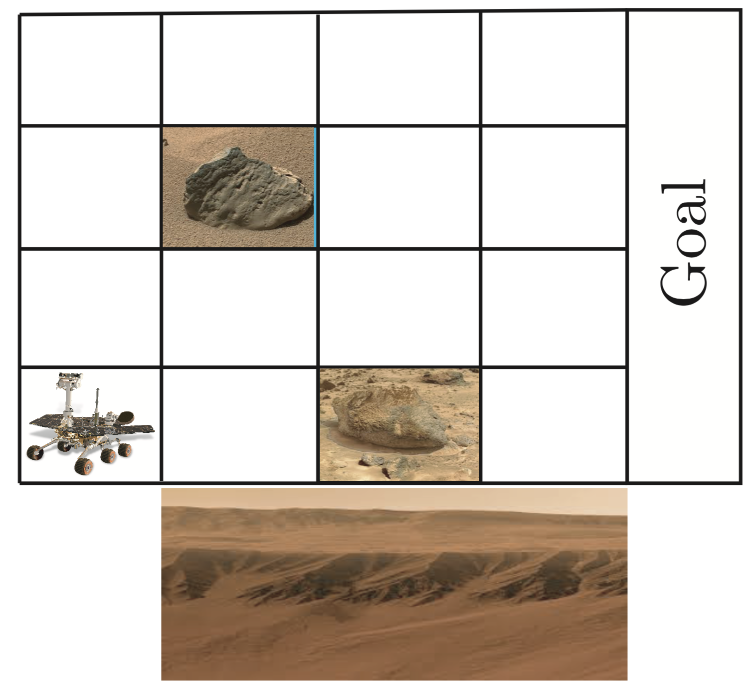
Formally, RockSample[] describes an instance of the problem with the terrain being a grid of size and rocks, which may have one of the types for . The rover may choose from the actions . When the rover moves off the right edge of the grid, it reaches its goal area, where it receives a reward of . Sampling of a rock yields a reward of if the rock is , and otherwise. The potentially negative reward causes an incentive to predict the type of a rock in advance. Executing action returns a noisy observation whether rock is or . The probability of a wrong observation decreases with the distance to rock . The underlying model is a POMDP, where the positions of the rover and the rock are observable, while the type of the rocks is not observable unless a rock has been sampled. The belief describe the probability of the correct rock types. To maximize the (expected) reward, the rover aims to correctly estimate the types in order to not sample a rock.
To account for the full potential of our method, we augmented the original RockSample problem as described above by (1) uncertainty and (2) safety considerations. First, concrete probabilities for wrong observations using the long-range sensor seem unrealistic when one considers that they may be the result of simulations and statistical inference of a probabilistic sensor model. Therefore, we introduce interval uncertainties. For instance, if from a certain distance there is a probability of for a faulty observation, we may assume that this probability lies within the interval to account for even worse accuracy of the sensor. A policy that maximizes the reward for the rover should then be robust against the uncertainties.
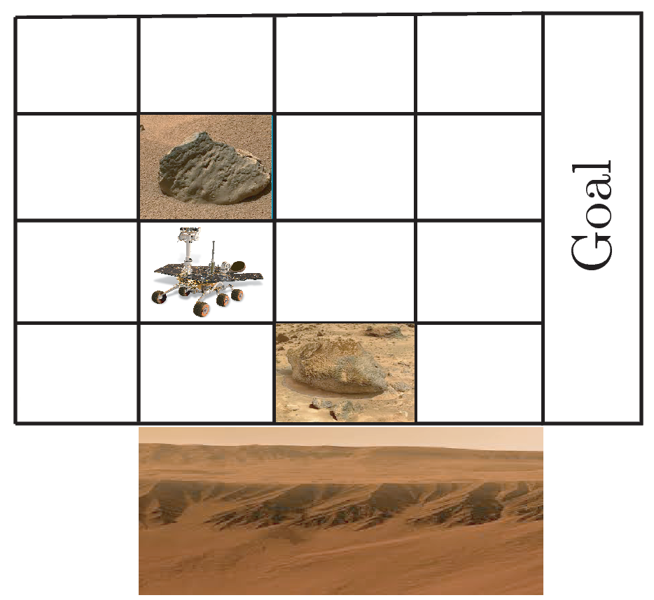
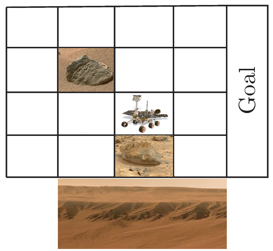
Secondly, we assume the rover has a certain probability to fall off a sand dune located at the bottom of the terrain. Safety considerations imply that the probability of falling off the dune should be less than . Such scenarios are commonly referred to as slippery grid worlds. The problem for a grid and rocks is depicted in Figure 3.
V-B Numerical Results
In our model, we assume the rock at the bottom of the grid is , and the other is .
V-B1 Case I
The first scenario we consider pertains to a policy that checks the type of the rocks from the initial state, then moves to the goal region after having sufficient confidence about the types of the rock according to a nominal observation probability. In order to model, the distance from the the rock positions and limited sensor accuracy, we assume the probability of having a correct observation belongs the interval and we set the nominal observation probability to . Given the policy designed for the nominal observation probability, our goal here is to find a lower bound on satisfying which lower-bounds the probability of identifying the rocks correctly. At the same time, we want to make sure that the rover does not move to the three slippery states at the bottom of the grid. We embed this safety constraint as . To this end, we construct two barrier certificate of fixed degree using Corollary 2 and perform a line search on the values of .
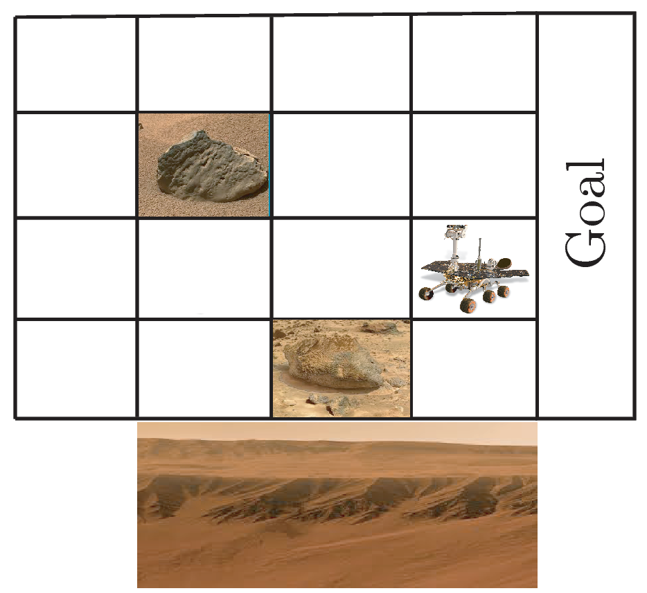
Table I demonstrates the results and shows that increasing the degree of the barrier certificates improves the accuracy of the lower bound. Experiments using PRISM and Storm also corroborate the consistency of these results. In the worst case of the uncertain observation probabilities, the nominal policy achieves the values of at and at . Figures (4.a) and (4.b) show two snapshots of how the Mars rover moves given this policy: the Mars rover stops at the initial position and use sensors to collect information about the rocks and then moves to the goal region.
| 1 | 2 | 3 | |
|---|---|---|---|
| 0.12 | 0.29 | 0.57 |
for . 1 2 3 0.31 0.44 0.73 for .
V-B2 Case II
We set the probability of having a correct observation to belong to the interval and the nominal probability is set to . The Mars rover is given a policy such that it first moves closer to the rocks, then checks the type of the rocks using the sensor, and moves to the goal after identifying the rock types. Figures (4.c) and (4.d) show two snapshots of the trajectory of the Mars rover over the grid using the nominal policy. In this case, we are interested to find lower bounds on and satisfying which corresponds to the belief in identifying each individual rock accurately.
Table II presents the results and demonstrates that increasing the degree of the barrier certificates enhances the lower bounds. These results tally with experiments in PRISM and Storm, which show that in the worst case, we have and .
| 1 | 2 | 3 | |
|---|---|---|---|
| 0.37 | 0.65 | 0.84 |
| 1 | 2 | 3 | |
|---|---|---|---|
| 0.32 | 0.73 | 0.89 |
|
 |
| (a) | (b) |
 |
 |
| (c) | (d) |
VI CONCLUSIONS AND FUTURE WORK
We proposed an approach for verifying the safety and/or optimality properties of POMDPs with uncertain transition/observation probabilities. The transition and/or observation uncertainties we considered belonged to fixed intervals. We cast the POMDP analysis problem into a switched system analysis problem and we brought forward a method based on barrier certificates. We showed that we can verify the satisfaction of optimality or safety requirements by computing a barrier certificate using sum-of-squares programming. We illustrated the applicability of our method on a Mars rover exploration example.
In this work, we considered the worst case analysis with the uncertain transition and/or observation probabilities. However, this analysis may be too conservative for problems where certain information about the transition/observation probabilities in terms of a probability density function is known. In this regard, the application of the scenario approach seems relevant [45]. Furthermore, the proposed method based on barrier certificates for verification of the POMDPs can also be used to synthesize policies ensuring both safety and optimality.
References
- [1] N. Meuleu, C. Plaunt, D. E. Smith, and T. Smith, “A POMDP for optimal motion planning with uncertain dynamics,” in ICAPS-10: POMDP Practitioners Workshop, 2010.
- [2] M. L. Puterman, Markov Decision Processes: Discrete Stochastic Dynamic Programming. John Wiley and Sons, 1994.
- [3] L. P. Kaelbling, M. L. Littman, and A. R. Cassandra, “Planning and acting in partially observable stochastic domains,” Artificial Intelligence, vol. 101, no. 1, pp. 99–134, 1998.
- [4] S. Thrun, W. Burgard, and D. Fox, Probabilistic Robotics. The MIT Press, 2005.
- [5] T. Wongpiromsarn and E. Frazzoli, “Control of probabilistic systems under dynamic, partially known environments with temporal logic specifications,” in CDC. IEEE, 2012, pp. 7644–7651.
- [6] S. J. Russell and P. Norvig, Artificial Intelligence: A Modern Approach, 2nd ed. Pearson Education, 2003.
- [7] G. Shani, J. Pineau, and R. Kaplow, “A survey of point-based POMDP solvers,” Autonomous Agents and Multi-Agent Systems, vol. 27, no. 1, pp. 1–51, 2013.
- [8] O. Madani, S. Hanks, and A. Condon, “On the undecidability of probabilistic planning and infinite-horizon partially observable Markov decision problems,” in AAAI. AAAI Press, 1999, pp. 541–548.
- [9] D. Braziunas, “Pomdp solution methods,” University of Toronto, Tech. Rep., 2003.
- [10] D. Szer and F. Charpillet, “An optimal best-first search algorithm for solving infinite horizon DEC-POMDPs,” in ECML. Springer, 2005, pp. 389–399.
- [11] G. Norman, D. Parker, and X. Zou, “Verification and control of partially observable probabilistic systems,” RTSS, vol. 53, no. 3, pp. 354–402, 2017.
- [12] N. Meuleu, C. Plaunt, D. E. Smith, and T. Smith, “A POMDP for optimal motion planning with uncertain dynamics,” in ICAPS-10: POMDP Practitioners Workshop, 2010.
- [13] J. A. Bagnell, A. Y. Ng, and J. G. Schneider, “Solving uncertain markov decision processes,” 2001.
- [14] B. Burns and O. Brock, “Sampling-based motion planning with sensing uncertainty.” IEEE, 2007, pp. 3313–3318.
- [15] H. Itoh and K. Nakamura, “Partially observable markov decision processes with imprecise parameters,” vol. 171, no. 8, pp. 453 – 490, 2007.
- [16] A. Bry and N. Roy, “Rapidly-exploring random belief trees for motion planning under uncertainty.” IEEE, 2011, pp. 723–730.
- [17] S. J. Russell, D. Dewey, and M. Tegmark, “Research priorities for robust and beneficial artificial intelligence,” CoRR, vol. abs/1602.03506, 2016.
- [18] D. Amodei, C. Olah, J. Steinhardt, P. Christiano, J. Schulman, and D. Mané, “Concrete problems in ai safety,” CoRR, vol. abs/1606.06565, 2016.
- [19] I. Stoica, D. Song, R. A. Popa, D. Patterson, M. W. Mahoney, R. Katz, A. D. Joseph, M. Jordan, J. M. Hellerstein, J. E. Gonzalez et al., “A berkeley view of systems challenges for ai,” CoRR, vol. abs/1712.05855, 2017.
- [20] R. G. Freedman and S. Zilberstein, “Safety in ai-hri: Challenges complementing user experience quality,” in AAAI Fall Symposium Series, 2016.
- [21] R. A. Howard, Dynamic Programming and Markov Processes. The MIT Press, 1960.
- [22] K. Chatterjee, M. Chmelík, and M. Tracol, “What is decidable about partially observable Markov decision processes with -regular objectives,” Journal of Computer and System Sciences, vol. 82, no. 5, pp. 878–911, 2016.
- [23] M. Hauskrecht, “Value-function approximations for partially observable markov decision processes,” J. Artif. Int. Res., vol. 13, no. 1, pp. 33–94, Aug. 2000.
- [24] M. T. J. Spaan and N. Vlassis, “Perseus: Randomized point-based value iteration for POMDPs,” J. Artif. Int. Res., vol. 24, no. 1, pp. 195–220, Aug. 2005.
- [25] O. Brock, J. Trinkle, and F. Ramos, SARSOP: Efficient Point-Based POMDP Planning by Approximating Optimally Reachable Belief Spaces. MIT Press, 2009, pp. 65–72.
- [26] M. J. Kochenderfer and J. P. Chryssanthacopoulos, “Collision avoidance using partially controlled Markov decision processes,” in Agents and Artificial Intelligence, J. Filipe and A. Fred, Eds. Springer, 2013, vol. 271, pp. 86–100.
- [27] T. Smith and R. Simmons, “Heuristic search value iteration for POMDPs,” in Proceedings of the 20th conference on Uncertainty in artificial intelligence. AUAI Press, 2004, pp. 520–527.
- [28] D. Liberzon, Switching in Systems and Control, ser. Systems & Control: Foundations & Applications. Birkhäuser Boston, 2003.
- [29] S. Prajna, A. Jadbabaie, and G. J. Pappas, “A framework for worst-case and stochastic safety verification using barrier certificates,” IEEE Transactions on Automatic Control, vol. 52, no. 8, pp. 1415–1428, Aug 2007.
- [30] M. Ahmadi, B. Wu, H. Lin, and U. Topcu, “Privacy verification in POMDPs via barrier certificates,” arXiv preprint arXiv:1804.03810, 2018.
- [31] E. J. Sondik, “The optimal control of partially observable Markov processes over the infinite horizon: Discounted costs,” Operations Research, vol. 26, no. 2, pp. 282–304, 1978.
- [32] K. J. Aström, “Optimal control of Markov decision processes with incomplete state estimation,” J. Math. Anal. Appl., vol. 10, pp. 174–205, 1965.
- [33] H. Itoh and K. Nakamura, “Partially observable Markov decision processes with imprecise parameters,” Artificial Intelligence, vol. 171, no. 8, pp. 453 – 490, 2007.
- [34] M. Ahmadi, G. Valmorbida, and A. Papachristodoulou, “Barrier functionals for output functional estimation of PDEs,” in 2015 American Control Conference (ACC), 2015, pp. 2594–2599.
- [35] ——, “Safety verification for distributed parameter systems using barrier functionals,” Systems & Control Letters, vol. 108, pp. 33 – 39, 2017.
- [36] P. Glotfelter, J. Cortés, and M. Egerstedt, “Nonsmooth barrier functions with applications to multi-robot systems,” IEEE Control Systems Letters, vol. 1, no. 2, pp. 310–315, Oct 2017.
- [37] M. Ahmadi, A. Israel, and U. Topcu, “Safety assessment based on physically-viable data-driven models,” in 2017 IEEE 56th Annual Conference on Decision and Control (CDC), Dec 2017, pp. 6409–6414.
- [38] M. Ahmadi, A. Israel, and U. Topcu, “Controller Synthesis for Safety of Physically-Viable Data-Driven Models,” ArXiv e-prints, Jan. 2018.
- [39] M. H. Stone, “Applications of the theory of Boolean rings to general topology,” Transactions of the American Mathematical Society, vol. 41, no. 3, pp. 375–481, 1937.
- [40] M. Kwiatkowska, G. Norman, and D. Parker, “Prism 4.0: Verification of probabilistic real-time systems,” in CAV, ser. LNCS, vol. 6806. Springer, 2011, pp. 585–591.
- [41] C. Dehnert, S. Junges, J. Katoen, and M. Volk, “A storm is coming: A modern probabilistic model checker,” in CAV, ser. LNCS, vol. 10427. Springer, 2017, pp. 592–600.
- [42] A. Megretski, “Systems polynomial optimization tools (SPOT),” 2010. [Online]. Available: https://github.com/anirudhamajumdar/spotless/tree/spotless_isos
- [43] A. A. Ahmadi and A. Majumdar, “DSOS and SDSOS optimization: more tractable alternatives to sum of squares and semidefinite optimization,” arXiv preprint arXiv:1706.02586, 2017.
- [44] A. A. Ahmadi, G. Hall, A. Papachristodoulou, J. Saunderson, and Y. Zheng, “Improving efficiency and scalability of sum of squares optimization: Recent advances and limitations,” in 2017 IEEE 56th Annual Conference on Decision and Control (CDC), Dec 2017, pp. 453–462.
- [45] M. C. Campi, S. Garatti, and M. Prandini, “The scenario approach for systems and control design,” Annual Reviews in Control, vol. 33, no. 2, pp. 149 – 157, 2009.
- [46] P. Parrilo, “Structured semidefinite programs and semialgebraic geometry methods in robustness and optimization,” Ph.D. dissertation, California Institute of Technology, 2000.
- [47] M. Choi, T. Y. Lam, and B. Reznick, “Sums of squares of real polynomials,” in Proceedings of Symposia in Pure mathematics, vol. 58. American Mathematical Society, 1995, pp. 103–126.
- [48] G. Chesi, A. Tesi, A. Vicino, and R. Genesio, “On convexification of some minimum distance problems,” in 5th European Control Conference, Karlsruhe, Germany, 1999.
- [49] M. Nie, J.and Schweighofer, “On the complexity of Putinar’s positivstellensatz,” Journal of Complexity, vol. 23, no. 1, pp. 135–150, 2007.
- [50] J. B. Lasserre, Moments, Positive Polynomials and Their Applications. Imperial College Press, London, 2009.
- [51] G. Chesi, “LMI techniques for optimization over polynomials in control: a survey,” IEEE Transactions on Automatic Control, vol. 55, no. 11, pp. 2500–2510, 2010.
-A Sum-of-Squares Polynomials
A polynomial is a sum-of-squares polynomial if , such that . Hence is clearly non-negative. A set of polynomials is called SOS decomposition of . The converse does not hold in general, that is, there exist non-negative polynomials which do not have an SOS decomposition [46]. The computation of SOS decompositions, can be cast as an SDP (see [46, 47, 48]). The Theorem below proves that, in sets satisfying a property stronger than compactness, any positive polynomial can be expressed as a combination of sum-of-squares polynomials and polynomials describing the set.
For a set of polynomials , , the quadratic module generated by is
| (24) |
A quadratic module is said archimedean if such that An archimedian set is always compact [49]. At this point, we recall the following result [50, Theorem 2.14].
Theorem 2 (Putinar Positivstellensatz)
Suppose the quadratic module is archimedian. Then for every ,
The subsequent proposition formalizes the problem of constrained positivity of polynomials which is a direct result of applying Positivstellensatz.
Proposition 1 ([51])
Let and belong to , then
| (25) | |||||
is satisfied, if the following holds
| (26) |
Proposition 2
The multivariable polynomial is strictly positive (), if there exists a such that
| (27) |
