Threshold $q$-voter model

Abstract

We introduce the threshold $q$-voter opinion dynamics where an agent, facing a binary choice, can change its mind when at least $q_{0}$ amongst $q$ neighbors share the opposite opinion. Otherwise, the agent can still change its mind with a certain probability $\varepsilon$. This threshold dynamics contemplates the possibility of persuasion by an influence group even when there is not full agreement among its members. In fact, individuals can follow their peers not only when there is unanimity ($q_{0}=q$) in the lobby group, as assumed in the $q$-voter model, but, depending on the circumstances, also when there is simple majority ($q_{0}>q/2$), Byzantine consensus ($q_{0}>2q/3$), or any minimal number $q_{0}$ amongst $q$. This realistic threshold gives place to emerging collective states and phase transitions which are not observed in the standard $q$-voter. The threshold $q_{0}$, together with the stochasticity introduced by $\varepsilon$, yields a phenomenology that mimics as particular cases the $q$-voter with stochastic drivings such as nonconformity and independence. In particular, nonconsensus majority states are possible, as well as mixed phases. Continuous and discontinuous phase transitions can occur, but also transitions from fluctuating phases into absorbing states.

I Introduction

In recent years, statistical physicists have proposed models of opinion dynamics to answer questions of current interest about public opinion formation such as the upraise of debate polarization, fragmentation or consensus review ; book1 ; book2 . In most of the models, individuals can adopt one of two opposite opinions. Although there are some real situations that require to contemplate several discrete Chen2005a ; Holme2006a ; plurality , or also continuous opinions Deffuant2000a ; Singh ; ramos2015a ; allan , the binary case constitutes the minimal setting to study opinion dynamics. The dual situation of deciding between two alternatives of similar attractiveness is faced in different scenarios, for instance, being favorable or unfavorable to a given proposal, or buying one of two similar products that compete in a market. Perhaps, the simplest binary opinion dynamics is given by the voter model, where each agent can flip its opinion by imitation (or contagion) of a randomly chosen neighbor review ; voter1 ; voter2 . In fact, imitation is a common and practical strategy for decision making, that shapes our behavior early in life imitation .

Contagion can be pairwise allan ; Biswas ; Crokidakis2014a ; Crokidakis2012a or involve group interactions ramos2015a ; Galam1986a ; Galam1997a ; Sznajd ; Galam2002a ; Krapivsky2003a ; Shao2009a ; q-voter . It can be outflow or inflow, that is, from the individual towards the neighbors or from the neighborhood towards the individual, respectively. In particular, Castellano et al. proposed an extension of the fundamental voter model, the nonlinear voter (or $q$-voter) model q-voter , where agents with binary opinions change mind when $q$ randomly chosen neighbors share the opposite opinion. This is a paradigmatic example of inflow group interaction that motivated the study of the evolution to consensus q-voter-1d ; q-voter-1D-exit ; q-voter-1D-exit2 , as well as the definition of variants of the original $q$-voter model, by introducing a probability of behaving as anticonformist, as stubborn, or of making random decisions q-voter-noises ; q-voter-zealots .

The voter models have been investigated mainly in complete graphs or regular lattices but also in more realistic heterogeneous networks 1-voter-complex1 ; 1-voter-complex2 ; uncorrelated ; javarone ; q-voter-complex1 ; mapping ; duplex ; deadlocksWS ; MFnetworks and co-evolving voter-coevolving1 ; voter-coevolving2 ; voter-coevolving3 ; voter-coevolving4 ; q-voter-coevolving networks.

Now, we introduce a generalization of the $q$-voter model, motivated by the consideration that $q_{0}$ (with $0\leq q_{0}\leq q$) of $q$ neighbors may be enough to change the opinion of an agent. In fact, individuals take decisions not only when there is unanimity ($q_{0}=q$) in the group of influencers but, depending on the circumstances, the Byzantine consensus ($q_{0}>2q/3$), the majority ($q_{0}>q/2$), or simply a minimal number $q_{0}$ following an idea among $q$ contacts may suffice. We will show that this realistic generalization leads to the appearance of collective states which are inaccessible through the $q$-voter dynamics, which only allows equal fraction of both opinions or total consensus.

The algorithm that defines this threshold opinion dynamics is introduced in Sec. II. The analytical approach based on a Fokker-Planck description is presented in Sec. III. Results from simulations together with analytical considerations are presented in Secs. IV and V and the Appendices. A summary and final remarks can be read in Sec. VI.

II Opinion dynamics

Although in principle the dynamics could be played in an arbitrary network of contacts, we consider a fully connected network of $N$ individuals. The opinions can have one of two different values, that we denote $\oplus$ and $\ominus$. The opinion of each individual can change influenced by a group of size $q$, according to the following algorithm:

1. An agent $i$ is selected at random.

2. Other $q$ agents are selected and their opinions are observed. Actually, repetitions are allowed. The possibility of repetitions mimics the fact that an individual can interact with a contact more than once.

3. If there are at least $q_{0}$ contrary opinions (where the threshold value is $0\leq q_{0}\leq q$), then, the opinion $o_{i}$ of agent $i$ is inverted, imitating the neighbors with contrary opinion.

4. Otherwise, the opinion of agent $i$ can also change with a probability $\varepsilon$, except if all in the $q$-lobby share the same opinion of site $i$.

When $q_{0}=q$, one recovers the nonlinear $q$-voter q-voter . In particular, $q_{0}=q=1$ leads to the original voter model.

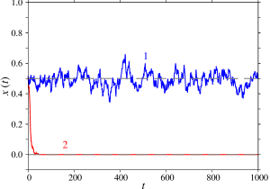
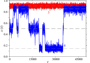
Figure 1: Temporal evolution of the fraction of $\oplus$ opinions $x(t)$. The parameters $(q,q_{0},\varepsilon)$ are 1: (4, 3, 0.42), 2: (4, 3 ,0.24), 3: (4, 3 ,0.30), 4: (8, 7 ,0.173). In all cases $N=1500$ and, in the initial state, there is equal number of agents with opposite opinions ($x(t=0)=1/2$). Dashed horizontal lines correspond to the minima of each potential $V(x)$ obtained by integration of Eq. (5).

Higher $q_{0}$ means individuals that are more hard to be convinced or less volatile. Typically $q_{0}>q/2$, meaning that a majority of neighbors is required to convince. The threshold $q_{0}$ can also be interpreted as the requirement of a critical mass of people sharing the opposite opinion to change mind. For completeness, we will analyze the model for any integer $0\leq q_{0}\leq q$. In the extreme case $q_{0}=0$, the selected agent changes mind no matter the opinion of the neighbors, that is, the individual acts as totally volatile, or independent.

The collective state can be characterized by the fraction of $\oplus$ opinions, $x(t)$. This is the relevant quantity that defines the opinion than wins. When $x=1/2$, there is balance of opinions, that is, a tie. Otherwise, one of the opinions wins, particularly full consensus occurs when $x=0$ or 1. Except if $q_{0}=0$, when consensus is reached, the dynamics freezes at that collective state. That is, consensus is an absorbing state.

The time evolution of the collective state $x(t)$, obtained by running computationally the algorithm defined above, is illustrated in Fig. 1, for different values of the parameters $(q,q_{0},\varepsilon)$. The unit of time $t$ corresponds to $N$ iterations of the algorithm. A diversity of behaviors emerges. The average opinion can fluctuate around zero (case 1), indicating polarization with equipartition of opposite opinions, technically a tie within finite-size fluctuations. The system can attain consensus (case 2). It can also evolve visiting non trivial collective states (cases 3 and 4), where one of the two opinions dominates, but without full consensus.

In order to understand the phenomenology of the dynamics, observed through numerical simulations, we will resort to a theoretical approach.

III Theoretical approach

A master equation for this problem can be derived along the lines of Ref. q-voter ; gardiner . In this binary scenario, there are two subpopulations with opposite opinions. Let us call $n$ the number of individuals with opinion $\oplus$ at a given instant. At an iteration of the algorithm (i)-(iv) defined in Sec. II, $n$ can change to $n^{\prime}$, with a certain rate that we call $p(n\to n^{\prime})$. The only possibilities with non null rate are $n^{\prime}=n+1,n,n-1$, since at most one flip of opinion happens at a time.

Moreover, we consider the probability of inversion $G(y)$, which is the probability that the opinion $o_{i}$ of the chosen agent flips, given that it belongs to the subpopulation with $yN$ individuals. That is, if $y=n/N$, then $G(y)$ gives the probability of flip from $\oplus$ to $\ominus$; while if $y=1-n/N$, then $G(y)$ gives the probability of flip from $\ominus$ to $\oplus$.

In terms of the probability of flip, the transition rates can be written as

$$p_{n\to n-1} = x\;G(x)\,,$$

$$p_{n\to n+1} = (1-x)\;G(1-x)\,,$$ (1)

$$p_{n\to n} = 1-p_{n\to n+1}-p_{n\to n-1}\,,$$

where $x\equiv n/N$.

According to the algorithm, the probability of flip is governed by the parameters $q$, $q_{0}$ and $\varepsilon$. A flip of $o_{i}$ occurs when the number of disagreeing neighbors exceeds a threshold $q_{0}$, but also, with chance $\varepsilon$ otherwise. Therefore the probability of a flip can be expressed as

$$G(y,q,q_{0},\varepsilon)=g(y,q,q_{0})+\varepsilon[1-g(y,q,q_{0})-y^{q}]\;,$$ (2)

where $g(y,q,q_{0})$ is the probability of having at least $q_{0}$ opposite opinions amongst $q$ randomly drawn ones, when agent $i$ is in the side with $yN$ individuals. This probability is given by the summation of the different favorable cases, i.e.,

$$g(y,q,q_{0})=\sum_{i=q_{0}}^{q}{{q}\choose{i}}(1-y)^{i}y^{q-i}\;.$$ (3)

Notice that, implicitly, repetitions are allowed, as defined in item (ii) of the algorithm. In Eq. (2), the term $y^{q}$ discounts the case where all agents in the influence group share the same opinion of agent $i$, as stated in item (iv) of the algorithm.

Once the transition rates are completely defined, we write a master equation that in the continuum limit can be approximated by a backward Fokker-Planck equation, namely,

$$\frac{\partial P}{dt^{\prime}}=v(x^{\prime})\frac{\partial P}{dx^{\prime}}+\frac{1}{2}D(x^{\prime})\frac{\partial^{2}P}{dx^{\prime 2}}\,,$$ (4)

where $P=P(x,t|x^{\prime},t^{\prime})$, the drift is

$$v(x)=(1-x)G(1-x,q,q_{0},\varepsilon)-xG(x,q,q_{0},\varepsilon),$$ (5)

and the diffusion coefficient is

$$D(x)=[(1-x)G(1-x,q,q_{0},\varepsilon)+xG(x,q,q_{0},\varepsilon)]/N\;.$$ (6)

Integrating Eq. (5), we obtain the potential $V(x)$, such that $v(x)=-dV/dx$, and we arbitrarily set the integration constant such that $V(0)=0$.

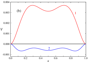
Figure 2: Potential $V(x)$. (a) $q=4$ and $q_{0}=3$, for different values of $\varepsilon$ indicated on the figure. The inset is a zoom of the interval $x\in[0,0.01]$. (b) $(q,q_{0},\varepsilon)=$ (4, 2, 0.12) and (8, 7, 0.173) for curves 1 and 2, respectively. Horizontal lines at $V=0$ are drawn for comparison.

Typical shapes of $V(x)$ are illustrated in Fig. 2, for different values of the parameters. In all cases $V(x)$ has symmetry around $x=1/2$ as expected, due to the symmetric role of opposite opinions. The potential profile determines the probability with which the system will dwell in each region of $0\leq x\leq 1$.

For sufficiently large $\varepsilon$, the potential presents a single minimum at $x=1/2$, which leads to the formation of a disordered state fluctuating around equipartition of opinions, like in case 1 of Fig. 1. At a particular value $\varepsilon_{1}$, the central minimum splits into two minima. This occurs when the second derivative of the potential $V(x)$ vanishes at the center. Using Eq. (5), to set the equation $V^{\prime\prime}(x=1/2)=-v^{\prime}(x=1/2)=0$, we obtain numerically $\varepsilon_{1}\simeq 0.39$ in the case of Fig. 2(a). Below that value, the system can dwell in a collective state where one of the opinions dominates, without full consensus (see case 3 of Fig. 1).

Further decreasing $\varepsilon$, we find another particular value, $\varepsilon_{2}$, at which the second derivative of the potential $V(x)$ vanishes at the borders. From Eq. (5), taking $V^{\prime\prime}(x=0)=-v^{\prime}(x=0)=0$, we obtain $\varepsilon_{2}=0.25$ in the case of Fig. 2(a). At this point, the extreme values at the borders become minima. Then, from any initial condition, the system will directly evolve (without jumping potential barriers) towards an absorbing state of consensus, like in case 2 of Fig. 1.

Moreover, depending on the values of $q$ and $q_{0}$, there are still other possible shapes of the potential, different from those shown in Fig. 2(a). For instance, in Fig. 2(b), for $q=8$ and $q_{0}=7$, three local minima arise. Then, a trajectory like in case 4 of Fig. 1 can be observed.

However, in all these examples, at longer times than those shown in the figure, the system will eventually evolve to consensus, more rapidly the smaller the system. But, how long does it take to reach the absorbing state depending on the model parameters? How does it depend on the system size? These questions will be answered in the following section.

IV Time to consensus

We measured the average time, $T(N,1/2)$, that a system of size $N$ takes to reach the absorbing state of consensus, when the initial condition is $x=1/2$ (equipartition of opinions). In Fig. 3, we plot the numerical values of $T$ as a function of $N$, choosing $(q,q_{0})=(4,3)$ and different values of $\varepsilon$. The data points were obtained through two different procedures, with good agreement between them. The filled symbols represent the results obtained by performing the direct average over 200 samples. Alternatively, the hollow symbols were obtained from a fitting procedure, applied to the probability density function (PDF) of the time to consensus, as described in the Appendix A. Succinctly, we plotted the mean value of the resulting PDF.

We observe that, in all cases, for finite $N$, it takes a finite time to reach consensus. Moreover, there is a critical value ($\varepsilon_{c}=\varepsilon_{2}=0.25$, in the case of the example) for which the consensus time increases with system size as a power law, namely, $T\sim N^{1/2}$. This is the same critical behavior observed in the $q$-voter model q-voter . However, as we will see in the next section they correspond to different kind of transitions. For $\varepsilon>\varepsilon_{c}$, in which case the potential presents at least one minimum localized outside the borders, the time increases exponentially. That is, following the Arrhenius law, since a potential barrier must be overcome to reach consensus. Otherwise, when there are no potential barriers to jump, the evolution towards consensus occurs exponentially fast (like in case 2 of Fig. 1), in a time scale that in average increases logarithmically with $N$.

In the next section, we will concentrate in the phases and transitions observed near the large size limit.

Figure 3: Consensus time $T(N,x=1/2)$ vs. $N$, for $q=4$, $q_{0}=3$ and different values of $\varepsilon$ indicated on the figure. Hollow symbols correspond to the average over 200 samples, and full symbols to the value of the parameter that represents the mean value of an exponential (for $\varepsilon>0.25$) or log-normal distribution (otherwise), obtained by a nonlinear curve fitting procedure (see Appendix A). The solid line corresponds to $T\sim N^{1/2}$ for comparison. The insets show the same data in log-linear and linear-log scales to exhibit the exponential and logarithmic growths, respectively.

V Large-size systems

The smaller $N$, the larger are the fluctuations of $x(t)$ and, the system can quickly reach the absorbing state of consensus, as can be observed in Fig. 3. Once consensus is reached, the system will be trapped there forever, unless an external perturbation takes the system out of that absorbing state.

In the thermodynamic limit (TL), fluctuations vanish, because according to Eq. (6), $D(x)\sim 1/N$, then consensus is not reached in a finite time. Moreover, if a stable nonconsensus state (corresponding to the bottom of a potential well at $x\neq 0,1$) is accessible from a given initial condition, the system will evolve towards that steady state and remain there forever.

Visiting different states, spontaneously, requires fluctuations. Thus, trajectories like in case 4 of Fig. 1 arise for sufficiently large but finite $N$ ($N=1500$ in the examples of the figure). These are the large-size systems whose evolution we will discuss in this section.

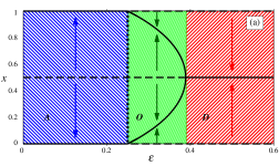
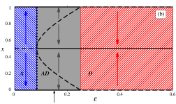
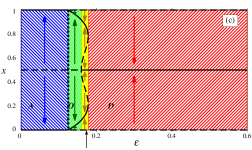
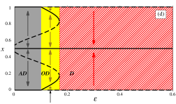
Figure 4: Stability diagrams in the plane $x$-$\varepsilon$, for $(q,q_{0})=$ (a) (4,3), (b) (4,2), (c) (8,7) and (d) (10,4). Solid (dashed) lines represent stable (unstable) values, corresponding to minima (maxima) of potential $V$. Each phase is represented by a different color and pattern: absorbing (A, blue), disordered (D, red), ordered (O, green), absorbing-disordered (AD, gray), ordered-disordered (OD, yellow). The arrows inside the diagrams show the direction of the evolution, towards stable points, depending on the initial condition. The arrows below the abscissa axis show the values of $\varepsilon$ at which all the minima are equally deep. The vertical dotted lines indicate the transitions for which $T(N)$ presents critical behavior as in Fig. 3.

In Fig. 4 we show stability diagrams in the plane $\varepsilon$-$x$ for different values of $q$ and $q_{0}$, chosen to illustrate diverse phases and transitions between them. The black lines correspond to the extreme values of the potential, given by $v(x)=0$, for each value of $\varepsilon$. Solid (dashed) lines correspond to the minima (maxima) of the potential, meaning stability (instability) of steady states. It is noteworthy that consensus ($x=0$ or $x=1$) is an absorbing state in this model, then independently of whether it is a maximum or minimum of the potential, once the system reaches consensus, it can not escape. In that sense, consensus is always stable. However, if it is a maximum (minimum) of the potential, then it will be unstable (stable) with respect to external perturbations.

In panel (a), notice that at small $\varepsilon$ the disordered state at $x=1/2$ is unstable while symmetric consensus states are stable. They loss stability beyond $\varepsilon=0.25$ where two stable nonconsensus steady values emerge. From the viewpoint of a dynamical system, these transitions correspond to trans-critical bifurcations. The stable steady states collide at $\varepsilon\simeq 0.39$, where the disordered state gains stability (super-critical pitchfork bifurcation). Three different phases can be identified:

“A” (absorbing phase, in blue): the system tends to consensus from any initial condition. It is associated to a potential $V(x)$ that presents only minima located at the borders.

“D” (disordered phase, in red): opposite opinions are equilibrated within fluctuations, like a paramagnetic phase in magnetic systems. It is associated to a single central minimum of the potential, at $x=1/2$.

“O” (ordered phase, in green): there is unbalance of opinions, like in a ferromagnetic phase. In this case, there is a majority or winner opinion. This phase is associated to the existence of two minima located at $x\neq 0,1/2,1$. For the $q$-voter model (where $q_{0}=q$), it has been argued q-voter that an ordered phase (that the authors call Ising-ferromagnetic, directed-percolation-active) might also occur for values $2<q<3$. However, this possibility is virtual in that model as soon as $q$ is integer, while in the threshold voter, the ordered phase can be effectively observed for integer values of $q$ and $q_{0}$.

In panel (b), there is stabilization of the disordered state at a critical value $\varepsilon=0.084$, in an inverse subcritical pitchfork bifurcation. At a second critical value $\varepsilon=0.25$, trans-critical bifurcations destabilize consensus states, while the disordered state remains stable. Between phases A and D, there is a mixed phase, in the sense that both phases A and D can be observed depending on the initial condition.

“AD”(absorbing-disordered, in gray): emerges from a sub-critical pitchfork bifurcation. There is metastability. From the lower critical value of $\varepsilon$ the minima associated to consensus are deeper, at an intermediate value (indicated by a vertical arrow below the abscissa axis) the central minimum becomes deeper.

In panel (c), between the phases O and D, we find another phase with metastability:

“OD” (ordered-disordered, in yellow), characterized by a central minimum and two minima out of the borders. That is, either the two symmetric ordered states or the disordered one can be reached depending on the initial condition. The stabilization of disorder occurs via an inverse subcritical pitchfork bifurcation, while the ordered states disappear due to a saddle-node bifurcation.

Finally, in panel (d), we observe transitions between phases AD and OD, which are trans-critical.

Notice that there are transitions involving absorbing states. Furthermore, between fluctuating phases, continuous and discontinuous transitions are possible. For instance, the transition between the phases O and D is continuous (see Fig. 4a), while the transition between OD and D is discontinuous (see Fig. 4d). In the latter case, hysteresis occurs, that is, the trajectories follow different paths when increasing and decreasing $\varepsilon$.

We did not detect a transition between the phases AD and O, which would require a flat potential, like in the voter transition, nor a mixed phase of the type AO (absorbing-ordered).

Phase diagrams in the plane $(q_{0}/q)$-$\varepsilon$, for all values of $q_{0}$, when $q=2,3,4,6,10$, are shown in Fig. 5. We will discuss some special cases in the next subsection.

In the phase diagrams, the thin black segments indicate the critical point $\varepsilon_{c}$ where the consensus time increases as a power law with $N$, namely $T\sim N^{1/2}$, delimiting the regimes where the consensus time increases exponentially (above $\varepsilon_{c}$) or logarithmically (below $\varepsilon_{c}$) with $N$. This critical behavior occurs between A and AD phases in the standard $q$-voter, while in this generalized version, the same critical behavior is additionally observed between phases A and O.

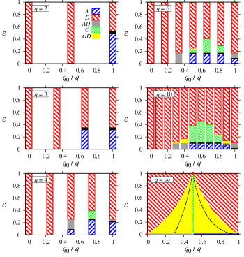
Figure 5: Phase diagram in the plane $(q_{0}/q)$-$\varepsilon$, for different values of $q$. Each phase is represented by a different color and pattern as in Fig. 4. The black thick segments in cases $q=2,3$, represent the voter transition. Thin black segments indicate the critical point where $T\sim N^{1/2}$. Last panel (results obtained in Appendix B for $q\to\infty$): the blue segment is where the potential is partially constant, and, at the dotted line, the three local minima of $V(x)$ possess the same value.

V.1 Unanimity voter ($q_{0}=q$)

The $q$-voter, for which $q_{0}=q$, corresponds to the last column of each plot in Fig. 5.

For $q=2$ (top panel), when $\varepsilon$ increases, we observe the direct passage from A to D, at $\varepsilon=1/2$. At that critical value, the potential is flat, $V(x)\equiv 0$, which corresponds to the voter transition, represented by a thick black segment. This transition also occurs for $q=3$ and $q_{0}=2,3$. In connection with the diagrams shown in Fig. 4, this transition can be interpreted as the collapse of the intermediate regions O in panel (a) or AD in panel (b), that disappear restoring the behavior with a single transition point.

For the higher lobby sizes $q=4,6,10$, we observe the appearance of the mixed phase AD (in gray) separating A and D, like in panel (b) of Fig. 4. This phase occurs for the interval $\varepsilon\in([q-1)]/[2^{q}-2],1/q)$. Its boundaries can be derived from the conditions $v^{\prime}(1/2)=0$ and $v^{\prime}(0)=0$, respectively.

Therefore, this domain has maximal length at $q=8$ and shrinks completely when $q\to\infty$ (see Appendix B). In that limit the voter transition is recovered (black circle).

For $q=1$ (voter model, not shown), the potential becomes flat, i.e., $V(x)\equiv 0$ for any $\varepsilon$.

V.2 Threshold voter $q_{0}\leq q$

When $q_{0}<q$, the new phases O and OD, absent in the standard $q$-voter, emerge.

The absorbing phase (A, blue) shrinks when $q$ increases, surviving for progressively lower levels of the stochasticity introduced by $\varepsilon$. This phase is absent for $q_{0}/q<1/2$, due to the disordering effect of the independent behavior associated to small $q_{0}$.

The emergence of the ordered (O, green) phase requires a minimal lobby size $q\geq 4$. For increasing $q$, this phase becomes narrower and more central in the plane $(q_{0}/q)-\varepsilon$, such that in the limit $q\to\infty$, it occurs for any $0<\varepsilon<1$ at $q_{0}=q/2$ only.

The order-disorder phase (OD, yellow) also appears for sufficiently large $q$ ($q\geq 6$). This domain grows for increasing $q$.

When $q_{0}=q/2$ (central columns in the panels of Fig. 5 for even $q$), the ordered phase O emerges for $q\geq 6$ within the interval $\varepsilon\in(1/q,\varepsilon_{\rm max})$, where $\varepsilon_{\rm max}$ increases with $q$, such that the ordered phase occupies all the interval $0<\varepsilon<1$ in the limit $q\to\infty$.

The case $q_{0}=0$ was also included for completeness, although this case is trivial since the phase is disordered for any $\varepsilon$. This is because step (iii) of the algorithm is always satisfied, then a flip is certain, leading to disorder. Moreover, since step (iii) is always satisfied when $q_{0}=0$, then step (iv) is never performed, hence the value of $\varepsilon$ is irrelevant.

V.3 Deterministic case $\varepsilon=0$

We start by discussing the large $q$ limit that admits simple analytical expressions. In the absence of the stochasticity introduced by $\varepsilon$, we find the AD phase (gray) for $q_{0}<q/2$ and the absorbing phase $A$ (blue) otherwise. But in this blue horizontal segment, there is an hybrid situation: from Eqs. (9) and (10), the central region of the potential is flat and the global minima are located at $x=0,1$. Only at $q_{0}=q/2$ the flat region disappears.

At the extreme values we have always disorder when $q_{0}=0$, while in the opposite case $q_{0}=q$, from Eq. (8), $g(x)\simeq 0$ in the limit of large $q$ and consequently $G(x)$ also vanishes, generating a flat potential $V(x)\equiv 0$.

For intermediate values of $q_{0}$, the three regions of the potential $V(x)$ behave as follows (see Appendix B: the lateral regions present their local minima at $x=\varepsilon/(1+\varepsilon)=0$, $x=1/(1+\varepsilon)=1$. The intermediate region has length $\left|1-2q_{0}/q\right|$ and presents different shapes for $q_{0}>q/2$ and $q_{0}<q/2$, respectively:

$V(x)=(1-q_{0}/q)^{2}/2$, i.e., it is constant.

$V(x)=x(x-1)+(1-q_{0}/[2q])q_{0}/q$, which is a quadratic function with a minimum at $x=1/2$.

Therefore, if $q_{0}\geq q/2$ consensus states are the only minima (phase A, blue), while, if $q_{0}<q/2$ there are three minima corresponding to consensus and disorder (phase AD, gray).

When $q$ is finite, we notice in Fig. 5, that the A region for $q_{0}\geq q/2$ is maintained, except for $q\leq 2$ while the AD region shrinks as $q$ decreases giving place to the disordered phase $D$ (red) at low $q_{0}$.

VI Summary and final remarks

In this paper, we introduced the threshold $q$-voter, a model of opinion formation in a dual decision scenario q-voter , which is an extension of the $q$-voter q-voter and consequently also of the voter model voter1 ; voter2 . The threshold $q_{0}$ is the minimal number, out of $q$ individuals forming an influence group, necessary to change the opinion of a randomly chosen agent. Like in the original version of the $q$-voter model, the agent can still change its mind with a probability $\varepsilon$, when the threshold condition is not satisfied.

We presented a characterization of the dynamics in the case of a fully-connected network. The threshold $q$-voter model exhibits a richer phenomenology than the standard $q$-voter, with new emergent phases, as can be observed in the phase diagram of Fig. 5. The disordered (D) and absorbing (A) phases that correspond to balance of opinions and consensus, respectively, and the mixed phase AD, where both collective states can occur depending on the initial condition, can be observed in the standard $q$-voter. In contrast, the threshold effect can drive the collective state towards a nonconsensus ordered phase O, with a winner opinion (case 4 of Fig. 1). This phase is not present in the $q$-voter model for the possible (integer) values of $q$. Moreover, a new mixed phase (OD) also emerges (case 3 of Fig. 1).

There are transitions involving absorbing states as in the $q$-voter, as well as new transitions between fluctuating phases. These can be continuous (like O-D) or discontinuous (like OD-D and OD-O) when changing parameter $\varepsilon$.

Beyond the original version of the $q$-voter model, variants have been introduced q-voter-noises by setting $\varepsilon=0$ and adding stochastic drivings: one representing anticonformism (where agents can disagree from the influence group with certain probability) and another representing independence (where agents can take a random decision with a certain probability). These drivings prevent consensus from being an absorbing state. This is in contrast to the threshold $q$-voter, where for any value of $q$ and $q_{0}$, a finite-size system reaches consensus in a finite time, as illustrated in Fig. 3. That is, the stochasticity introduced by $\varepsilon$ hampers order but it does not prevent consensus from being an absorbing state, while the occurrence of independent and anticonformist decisions can take the system out from consensus due to random flips. Also notice that, although flipping by $\varepsilon$ can be associated to random decision making independently of the neighbors norm, it occurs in step (iv) of the algorithm, only if the threshold condition is not satisfied. Therefore, in particular, when there is consensus there can not be flips, except if $q_{0}=0$, hence consensus is an absorbing state. When $q_{0}=0$, step (iii) of the algorithm is always satisfied, then flipping is certain, leading to a disordered state, and step (iv) is never executed, independently of $\varepsilon$. Since the chosen agent changes mind no matter the opinion of the neighbors, it acts independently of the state of the influence group. Although attenuated, this effect still occurs as $q_{0}$ increases up to $q/2$.

Certain analogies can be established between the threshold $q$-voter with $\varepsilon\neq 0$ and the variants with independence and anticonformism as defined above. For certain values of the flipping probability, both produce the ordered phase O, while the mixed phase OD is observed in the case of independence.

Enhancing independence leads to the transitions O-OD-D q-voter-noises (green-yellow-red regions in Fig. 5). Looking at Fig. 5, one sees that this sequence occurs for sufficiently large $q$, for instance, in the case $q=10$, setting $\varepsilon\simeq 0.1$ and decreasing $q_{0}$, which in fact we have associated to increasing level of independence. The sequence also occurs by increasing $q_{0}$, from central values. In fact, if $q_{0}$ is large, it is difficult to satisfy the threshold condition and have a flip in step (iii) of the algorithm, because an agent needs to see almost unanimity in its neighborhood to change its mind. But then the algorithm proceeds to step (iv) and a flip in this step also represents a random change of opinion, independent of the dominant opinion in the influence group.

Increasing anticonformity promotes the transition O-D q-voter-noises (green-red in Fig. 5). In our model, this transition occurs typically for not too large $q$. For instance by starting from central values of $q_{0}$ and increasing $\varepsilon$. When $q_{0}$ is central, step (iii) of the algorithm is not implemented when there is a minority with opposite opinion, then a flip can occur in step (iv) leading to share the opinion of the minority, mimicking anticonformity or contrarian decisions. This effect increases with $\varepsilon$, then this parameter emulates the probability of the anticonformist driving.

Therefore, the interplay between the threshold $q_{0}$ and the stochastic effect controlled by $\varepsilon$ yields as particular cases the phenomenologies observed under the inclusion of independence or anticonformity.

Let us also remark that consensus is always reached as a final state in the present model. However, while for $\varepsilon$ below a critical value $\varepsilon_{c}$ the time to consensus increases logarithmically with system size $N$, above $\varepsilon_{c}$, the growth is exponential. As a consequence, a large system in a mixed phase can visit metastable states before reaching consensus. The emergence of metastability is particularly important in this context, because if the global opinion of a population can spontaneously change from one metastable state to another, then the result of the election will depend on the precise moment it occurs, differently to the case where there is a unique steady state. Moreover, a perturbation, like propaganda might easily switch the state of the system, redefining the result of the election.

Finally, let us comment that the original voter, $q$-voter and their variants have been been studied not only in complete graphs and regular lattices, but also in diverse more realistic heterogeneous networks, such as Watts-Strogatz, Barabasi-Albert, random regular or even real networks (for the definition of these networks see for instance  networks ). For the voter model, it was shown how network structure affects the $N$-dependence of the consensus time 1-voter-complex1 ; 1-voter-complex2 ; uncorrelated . For the $q$-voter, it was also shown that the consensus reaching process is facilitated by properties such as long-range interactions mapping , randomness and density of a network deadlocksWS ; MFnetworks . Moreover structure can also change the nature of phase transitions, like in duplex clique graphs duplex . Therefore, as a perspective of future work, it would be interesting to analyze the role of a topology in the threshold $q$-voter dynamics. Also interesting would be the study in co-evolving networks extending previous results for voter models voter-coevolving1 ; voter-coevolving2 ; voter-coevolving3 ; voter-coevolving4 ; q-voter-coevolving where in addition to consensus and coexistence, fragmentation of the network can emerge depending on the rewiring probability.

Appendix A Consensus time distribution

Consensus time probability density functions (PDFs), estimated from the results of simulations, are exemplified in Fig. 6. For $\varepsilon>\varepsilon_{c}$ [see Fig. 6(a)], the numerical result can be well described by the exponential PDF $f(x)={\rm e}^{-x/\tau}/\tau$, while for $\varepsilon<\varepsilon_{c}$ [see Fig. 6(a)], the time to consensus can be described by a log-normal PDF $f(x)={\rm e}^{-[\ln(x/x_{c})]^{2}/(2w^{2})}/(x\,w\,\sqrt{2\pi})$, where $\tau,w,x_{c}$ are real parameters.

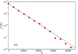
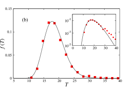
Figure 6: Probability density distribution of the time to consensus, for $(q,q_{0})=(4,3)$, in which case $\varepsilon_{c}=0.25$, $\varepsilon=0.30$ (a) and 0.15 (b). In both cases, the population size is $N=1000$. The symbols correspond to normalized histograms built from $10^{4}$ realizations. The dotted lines correspond to a fit of exponential (with $\tau\simeq 10^{4}$) and log-normal (with $w\simeq 0.18$ and $x_{c}\simeq 18.3$) distributions, respectively.

In the exponential case, there is a single fitting parameter value $\tau$, which represents the mean, as well as the standard deviation. In the case of the log-normal PDF, there are two fitting parameters $w$ and $x_{c}$, associated to the mean value $x_{c}\,{\rm e}^{w^{2}/2}$ and the standard deviation $(x_{c})^{2}{\rm e}^{w^{2}}({\rm e}^{w^{2}}-1)$. A standard nonlinear curve fitting procedure was used. The distribution works well in the central part but the tail decays more slowly. The full symbols in Fig. 3 represent the average time obtained from fittings, that is $T=\tau$ and $T=x_{c}\,{\rm e}^{w^{2}/2}$ for exponential and log-normal PDFs, respectively. These estimates are in good agreement with the direct average of the consensus time recorded for 200 samples (hollow symbols).

Appendix B Large lobby size limit

For very large $q$, we can perform the following approximations. The summation in Eq. (3) can be substituted by an integral and the binomial factor by its Gaussian approximation. By integrating the resulting expression from $q_{0}$ to $q$, we obtain

$$g(x,q,q_{0})\sim\frac{1}{2}\left\{1-{\rm erf}\left[\frac{q_{0}-q(1-x)}{[2q(1-x)x]^{1/2}}\right]\right\}\,.$$ (7)

In turn, in the limit $q\rightarrow\infty$, the error function (erf) can be approximated by the sign function (sgn), where ${\rm sgn}(x)=2H(x)-1$, being $H(x)$ the Heaviside step function. Then, we get

$$g(x,q,q_{0})\simeq\frac{1}{2}\left\{1-{\rm sgn}\left[\frac{q_{0}}{q}-(1-x)\right]\right\}~{}.$$ (8)

Computing $V(x)=-\int_{0}^{x}v(y)dy$, from Eq. (5), we obtain

$$V(x)=\left\{\begin{array}[]{ll}-\varepsilon x\left(1-\frac{x}{2}\right)+\frac{x^{2}}{2}~{},&x\in[0,1-\frac{q_{0}}{q}],\\ \frac{(1-\varepsilon)}{2}\left(1-\frac{q_{0}}{q}\right)^{2}-\varepsilon x(1-x)~{},&x\in[1-\frac{q_{0}}{q},\frac{q_{0}}{q}],\\ \frac{(1-\varepsilon)}{2}-x\left(1-\frac{x}{2}\right)+\varepsilon\frac{x^{2}}{2}~{},&x\in[\frac{q_{0}}{q},1],\end{array}\right.$$ (9)

for $\frac{q_{0}}{q}\in[\frac{1}{2},1]$, and

$$V(x)=\left\{\begin{array}[]{ll}-\varepsilon x\left(1-\frac{x}{2}\right)+\frac{x^{2}}{2}~{},&x\in[0,\frac{q_{0}}{q}],\\ (1-\varepsilon)\frac{q_{0}}{q}\left(1-\frac{q_{0}}{2q}\right)-x(1-x)~{},&x\in[\frac{q_{0}}{q},1-\frac{q_{0}}{q}],\\ \frac{(1-\varepsilon)}{2}-x\left(1-\frac{x}{2}\right)+\varepsilon\frac{x^{2}}{2}~{},&x\in[1-\frac{q_{0}}{q},1],\end{array}\right.$$ (10)

when $\frac{q_{0}}{q}\in[0,\frac{1}{2}]$.

Analyzing the extrema of $V(x)$, we can delimit the regions in the phase diagram. Taking $dV/dx=0$ in Eqs. (9) and (10), we determine that there are at most three local minima localized at $x=\varepsilon/(1+\varepsilon),1/2,1/(1+\varepsilon)$, if these values belong to the corresponding intervals. The fact that in the large $q$ limit we obtain at most three minima suggests that this is the maximal number of minima in the interval $x\in[0,1]$, for any finite $q$, despite the potential can be a higher order polynomial. Moreover, for $q=50$, sweeping $\varepsilon$, for all $q_{0}$, we did not detect any region with more minima of the potential.

In the lower panel of Fig. 5, we present the phase diagram in this limit. Inside the OD region (yellow), where the potential has three minima, the dotted line represents the points where the potential $V$ has the same value at the three minima. Above the dotted line, the central minimum becomes deeper.

The boundary between OD and D phases is described by

$$\varepsilon_{c}=\left\{\begin{array}[]{cl}q_{0}/(q-q_{0})\,,&\quad 0\leq q_{0}/q\leq 1/2\,,\\ q/q_{0}-1\,,&\quad 1/2\leq q_{0}/q\leq 1\,,\\ \end{array}\right.$$ (11)

obtained by the condition that the lateral minima are at the interior borders of the corresponding intervals.

The O phase became restricted to the central vertical segment at $x=1/2$.

Differently, in the $q$-voter case, for very large $q$, only disorder is possible, except when $\varepsilon=0$, in which case one observes the same behavior that in the voter model.

Acknowledgments: We acknowledge Brazilian agencies CNPq and FAPERJ for partial financial support.

Note: After publication, we became aware of Ref.  threshold-sznajd , where a threshold is also introduced in the $q$-voter model. However, these results do not overlap with ours since, besides different approaches are used, the model of Ref. threshold-sznajd sets $\varepsilon=0$, including independence and anti-conformity instead.

References

- (1) S. Galam, Sociophysics: A Physicist’s Modeling of Psycho-Political Phenomena, Springer, Berlin (2012).
- (2) P. Sen, B.K. Chakrabarti, Sociophysics: An Introduction, Oxford University Press, Oxford (2014).
- (3) C. Castellano, S. Fortunato, and Vittorio Loreto, Rev. Mod. Phys. 81, 591 (2009).
- (4) P. Chen, S. Redner, J. Phys. A 38, 7239 (2005).
- (5) P. Holme, M.E.J. Newman, Phys. Rev. E 74, 056108 (2006).
- (6) A. M. Calvão, M. Ramos and C. Anteneodo, J. Stat. Mech. 023405 (2016).
- (7) G. Deffuant, D. Neau, F. Amblard, G. Weisbuch, Adv Complex Syst. 3, 87 (2000).
- (8) P. Singh, S. Sreenivasan, B.K. Szymanski, G. Korniss, Sci. Rep. 3, 2330 (2013).
- (9) M. Ramos, J. Shao, S.D.S. Reis, C. Anteneodo, J.S. Andrade Jr, S. Havlin S, H. Makse, Scientific reports 5, 10032 (2015).
- (10) A.R. Vieira, C. Anteneodo, N. Crokidakis, JSTAT 023204 (2016).
- (11) P. Clifford and A. Sudbury, Biometrika, 60, 581 (1973).
- (12) R. A. Holley and T. M. Liggett, Ann. Prob. 3, 643 (1975).
- (13) M.J. Salganik, D.J. Watts, Topics in Cognitive Science 1, 439 (2009).
- (14) S. Biswas, A. Chatterjee, P. Sen, Physica A 391, 3257 (2012).
- (15) N. Crokidakis, V.H. Blanco, C. Anteneodo, Phys. Rev. E 89, 013310 (2014).
- (16) N. Crokidakis, C. Anteneodo, Phys. Rev. E 86, 061127 (2012).
- (17) S. Galam, J. Math. Psychol. 30, 426 (1986).
- (18) S. Galam, Physica A 238, 25 (1997).
- (19) K. Sznajd-Weron, J. Sznajd, Int. J. Mod. Phys. C. 11, 1157 (2000).
- (20) S. Galam, Eur. Phys. J. B 25, 403 (2002).
- (21) P.L. Krapivsky, S. Redner, Phys. Rev. Lett. 90, 238701 (2003).
- (22) J. Shao, S. Havlin, H.E. Stanley, Phys. Rev. Lett. 103, 018701 (2009).
- (23) C. Castellano, M. A. Muñoz and R. Pastor-Satorras, Physical Review E 80, 041129 (2009).
- (24) P. Przybyla, K. Sznajd-Weron, and M. Tabiszewski, Phys. Rev. E 84, 031117 (2011).
- (25) A.M. Timpanaro, C. P. C. Prado, Phys. Rev. E 89, 052808 (2014).
- (26) A. M. Timpanaro and S. Galam, Phys. Rev. E 92, 012807 (2015).
- (27) P. Nyczka, K. Sznajd-Weron, and J. Cisło, Phys. Rev. E 86, 011105 (2012).
- (28) M. Mobilia, Phys. Rev. E 92, 012803 (2015).
- (29) V. Sood and S. Redner, Phys. Rev. Lett. 94, 178701 (2005).
- (30) V. Sood, T. Antal, and S. Redner, Phys. Rev. E 77, 041121 (2008).
- (31) F. Vazquez and V. M. Eguíluz, New J. Phys. 10, 063011 (2008).
- (32) M. A. Javarone, and T. Squartini, J. Stat. Mech.: Theory Exp. P10002 (2015).
- (33) A. Jedrzejewski, Phys. Rev. E 95, 012307 (2017).
- (34) A. Jedrzejewski, K. Sznajd-Weron, and J. Szwabinski, Physica A 446, 110 (2016).
- (35) A. Chmiel and K. Sznajd-Weron, Phys. Rev. E 92, 052812 (2015).
- (36) K. Sznajd-Weron and K.M. Suszczynski, J. Stat.Mech.: Theory Exp. (2014) P07018.
- (37) P. Moretti, S. Liu, C. Castellano, and R. Pastor-Satorras, J. Stat. Phys. 151, 113 (2013).
- (38) D. Kimura and Y. Hayakawa, Phys. Rev. E 78, 016103 (2008).
- (39) F. Vazquez, V. M. Eguíluz, and M. San Miguel, Phys. Rev. Lett. 100, 108702 (2008).
- (40) C. Nardini, B. Kozma, and A. Barrat, Phys. Rev. Lett. 100, 158701 (2008).
- (41) G. Demirel, F. Vazquez, G. Böhme, and T. Gross, Physica D 267, 68 (2014).
- (42) B. Min, M.San Miguel, Scientific Reports 7, 12864 (2017).
- (43) C. W. Gardiner, Handbook of Stochastic Methods, 2nd ed., Springer, Berlin (1985).
- (44) S. Boccaletti, V. Latora, Y. Moreno, M. Chavez, D.-U.Hwang, Physics Reports 424, 175 (2006).
- (45) P. Nyczka, K. Sznajd-Weron, J. Stat. Phys. 151, 174 (2013).