Potentially observable cylindrical wormholes
without exotic matter in general relativity

K. A. Bronnikov
Center for Gravitation and Fundamental Metrology, VNIIMS, Ozyornaya 46, Moscow 119361, Russia;
Institute of Gravitation and Cosmology, Peoples’ Friendship University of Russia (RUDN University),
          ul. Miklukho-Maklaya 6, Moscow 117198, Russia;
National Research Nuclear University “MEPhI” (Moscow Engineering Physics Institute),
          Kashirskoe sh. 31, Moscow 115409, Russia

V. G. Krechet
Moscow State Technological University “Stankin”, Vadkovsky per. 3A, Moscow 127055, Russia

All known solutions to the Einstein equations describing rotating cylindrical wormholes lack asymptotic flatness in the radial directions and therefore cannot describe wormhole entrances as local objects in our Universe. To overcome this difficulty, wormhole solutions are joined to flat asymptotic regions at some surfaces $\Sigma_{-}$ and $\Sigma_{+}$. The whole configuration thus consists of three regions, the internal one containing a wormhole throat, and two flat external ones, considered in rotating reference frames. Using a special kind of anisotropic fluid respecting the Weak Energy Condition (WEC) as a source of gravity in the internal region, we show that the parameters of this configuration can be chosen in such a way that matter on both junction surfaces $\Sigma_{-}$ and $\Sigma_{+}$ also respects the WEC. Closed timelike curves are shown to be absent by construction in the whole configuration. It seems to be the first example of regular twice (radially) asymptotically flat wormholes without exotic matter and without closed timelike curves, obtained in general relativity.

1 Introduction

Traversable Lorentzian wormholes are widely discussed in gravitational physics since they lead to many effects of interest like time machines or shortcuts between distant parts of space. Large enough wormholes, if any, can lead to observable effects in astronomy [1, 2, 3, 4].

In attempts to build realistic wormhole models, the main difficulty is that in general relativity (GR) and some of its extensions a static wormhole geometry requires the presence of “exotic”, or phantom matter, that is, matter violating the weak and null energy condition (WEC and NEC), at least near the throat, the narrowest place in a wormhole [5, 6, 7, 8]. These results were obtained if the throat is a compact 2D surface with a finite area [7]. Assuming asymptotic flatness and fulfillment of the averaged NEC, topological restrictions have been proven [9, 10, 11] that forbid the existence of wormholes having two flat asymptotic regions (the so-called topological censorship).

Examples of phantom-free wormhole solutions are known in extensions of GR, such as the Einstein-Cartan theory [12, 13], Einstein-Gauss-Bonnet gravity [14], brane worlds [15] and other multidimensional models [16], etc. We here prefer to adhere to GR as a theory well describing the macroscopic reality while the extensions more likely concern very large densities and/or curvatures. In GR there are phantom-free wormhole models with axial symmetry, such as the Zipoy [17] and superextremal Kerr vacuum solutions as well as solutions with scalar and electromagnetic fields [18, 19]; in all of them, however, a disk that plays the role of a throat is bounded by a ring singularity whose existence is a kind of unpleasant price paid for the absence of exotic matter. Regular phantom-free wormholes in GR were found in [20, 21], sourced by a nonlinear sigma model, but they are asymptotically NUT-AdS instead of the desired flatness. A phantom-free wormhole construction in [22] contains singularities and closed timelike curves. These shortcomings may be interpreted as manifestations of topological censorship.

The above-mentioned results of [7] as well as topological censorship are not directly applicable to objects like cosmic strings, infinitely stretched along a certain direction, in the simplest case cylindrically symmetric ones. Thus, for example, nontrivial stationary cylindrically symmetric systems cannot be completely asymptotically flat since in the longitudinal ($z$) direction, due to $z$-independence, at large $z$ the curvature is the same as at small $z$, and which is important, such nonzero curvature is preserved along null ($z,t$) directions owing to time independence. In other words, all nontrivial cylindrically symmetric systems are not asymptotically flat in the usual sense. And it is this circumstance that gives us a hope to obtain a wormhole without exotic matter that will be asymptotically flat  in the remaining two spatial directions (or, which is the same, in the radial direction) on both sides of the throat (maybe up to an angular deficit, as in cosmic strings), which is necessary if we wish it to be potentially visible to distant observers like ourselves residing in weakly curved regions of the Universe.

We can remark that cylindrical symmetry was used for many decades as a kind of theoretical laboratory, where one could ask, for example, what can happen under extremely large deviations from spherical symmetry, or study anisotropic cosmological models. The corresponding isometry group provides many mathematical results of interest (see, e.g., [30] and references therein). On the other hand, the fields of some natural objects (jets, filament-like structures etc.) may be approximately described as cylindrically symmetric ones in some restricted region. However, studies with this symmetry have gained much more interest and popularity since the theoretical discovery of cosmic strings, leading to attempts to find them in the Universe and to use them for solving a number of astrophysical and cosmological problems [31]. Cylindrical wormholes, if any, may look like cosmic strings for a distant observer.

Cylindrical wormholes with and without rotation were discussed, in particular, in [23, 24, 27, 26, 25] (see also references therein). It was shown, with a number of examples, that phantom-free cylindrical wormhole solutions to the Einstein equations are easily obtained. A problem with cylindrical systems is, as in [20, 21], their undesirable asymptotic behavior. This does not look unexpected since even in Newtonian theory the gravitational potential of a cylindrical body grows logarithmically at large radii, and its relativistic counterpart, the Levi-Civita vacuum solution [28], has similar properties. The majority of papers devoted to cylindrical systems in gravity theories do not care of a possible even partial asymptotic flatness, frequently discussing matter distributions matched to the Levi-Civita (or Lewis [29]) external solutions. Our study (as well as [24, 25, 26]) has the advantage that the requirement of radial asymptotic flatness is our basic concern, and it is a maximum of what could be required under cylindrical symmetry.

To overcome this difficulty with cylindrical wormhole solutions and to provide radial asymptotic flatness, it was suggested [24] to cut such a solution on some surfaces (cylinders) $\Sigma_{-}$ and $\Sigma_{+}$ on both sides of the throat and to join them to suitable parts of Minkowski space-time, ${\mathbb{M}}_{-}$ and ${\mathbb{M}}_{+}$. Each of the latter should have a spatial part in the form of Euclidean space with a cut-out straight tube of finite radius. The surfaces $\Sigma_{-}$ and $\Sigma_{+}$ then contain some matter whose stress-energy tensor (SET) components $S_{a}^{b}$ are determined by the junction conditions in terms of jumps of the extrinsic curvature [34, 35]. A wormhole model without exotic matter is thus built if matter in the internal region and the surface matter on both $\Sigma_{-}$ and $\Sigma_{+}$ respect the WEC. No successful examples of phantom-free wormholes were so far obtained in this way. Moreover, it was shown that many kinds of matter filling the internal region create such geometry that it is impossible to obtain $S_{a}^{b}$ satisfying the WEC on both junctions $\Sigma_{\pm}$ [25, 26].

In the present paper we show that this goal is achieved if we use a special kind of anisotropic fluid as a source of gravity in the internal region. In the next section we obtain the internal solution, in Section 3 we consider its matching to flat external regions and show that the whole model satisfies the WEC under a proper choice of the free parameters. Section 4 contains a discussion of a difficulty emerging due to different signs of the angular velocity of rotation $\Omega$ in ${\mathbb{M}}_{+}$ and ${\mathbb{M}}_{-}$. The problem emerges if we try to replace a thin shell with a smooth matter distribution: in the latter, described in its comoving reference frame, the rotational direction cannot change from one layer to another. A suggested way out is to use the fact that in vacuum all reference frames are comoving. The Appendix contains a calculation related to this discussion: it is shown that using the presently studied wormhole solution, it is impossible to obtain the same sign of $\Omega$ in both $\Sigma_{+}$ and $\Sigma_{-}$.

2 Wormhole solution
with an anisotropic fluid

Consider a stationary cylindrically symmetric metric

$${}ds^{2}={\,\rm e}^{2\gamma(x)}[dt-E(x){\,\rm e}^{-2\gamma(x)}\,d\varphi]^{2}-{\,\rm e}^{2\alpha(x)}dx^{2}$$

$${}\hskip 28.45274pt-{\,\rm e}^{2\mu(x)}dz^{2}-{\,\rm e}^{2\beta(x)}d\varphi^{2},$$ (1)

where $x$, $z$ and $\varphi$ are the radial, longitudinal and angular coordinates. This metric is said to describe a wormhole if either (i) the circular radius $r(x)={\,\rm e}^{\beta(x)}$ has a regular minimum (called an $r$-throat) and is large or infinite far from this minimum or (ii) the same is true for the area function $a(x)={\,\rm e}^{\mu+\beta}$ (its minimum is called an $a$-throat) [23, 24]. If a wormhole is asymptotically flat at both extremes of the $x$ range, it evidently possesses both kinds of throats.

The metric coefficient $g_{03}=-E$ corresponds to space-time rotation which can be characterized by the angular velocity $\omega(x)$ of a congruence of timelike curves [24, 32, 33],

$$\omega={{\textstyle\frac{1}{2}}}(E{\,\rm e}^{-2\gamma})^{\prime}{\,\rm e}^{\gamma-\beta-\alpha}.$$ (2)

(this expression holds under an arbitrary choice of the coordinate $x$, and a prime stands for $d/dx$). Furthermore, in the reference frame comoving to matter in its motion by the angle $\varphi$ we have the SET component $T^{3}_{0}=0$, hence (via the Einstein equations) we have the Ricci tensor component $R_{0}^{3}\sim(\omega{\,\rm e}^{2\gamma+\mu})^{\prime}=0$, so that [24]

$$\omega=\omega_{0}{\,\rm e}^{-\mu-2\gamma},\hskip 28.45274pt\omega_{0}={\rm const}.$$ (3)

Then, according to (2),

$$E(x)=2\omega_{0}{\,\rm e}^{2\gamma(x)}\int{\,\rm e}^{\alpha+\beta-\mu-3\gamma}dx.$$ (4)

It then turns out [24] that the diagonal components of the Ricci ($R_{\mu}^{\nu}$) and Einstein ($G_{\mu}^{\nu}=R_{\mu}^{\nu}-{{\textstyle\frac{1}{2}}}\delta_{\mu}^{\nu}R$) tensors split into those for the static metric (that is, (2) with $E=0$) plus an $\omega$-dependent addition:

$$R_{\mu}^{\nu} = {}_{s}R_{\mu}^{\nu}+{}_{\omega}R_{\mu}^{\nu},\qquad G_{\mu}^{\nu}={}_{s}G_{\mu}^{\nu}+{}_{\omega}G_{\mu}^{\nu},$$

$${}{}_{\omega}R_{\mu}^{\nu} = \omega^{2}\mathop{\rm diag}\nolimits(-2,2,0,2),$$

$${}{}_{\omega}G_{\mu}^{\nu} = \omega^{2}\mathop{\rm diag}\nolimits(-3,1,-1,1),$$ (5)

where ${}_{s}R_{\mu}^{\nu}$ and ${}_{s}G_{\mu}^{\nu}$ are the static parts. The tensors ${}_{s}G_{\mu}^{\nu}$ and ${}_{\omega}G_{\mu}^{\nu}$ (each separately) satisfy the conservation law $\nabla_{\alpha}G^{\alpha}_{\mu}=0$ in terms of this static metric. Thus, by the Einstein equations $G_{\mu}^{\nu}=-\varkappa T_{\mu}^{\nu}$ ($\varkappa=8\pi G$), the tensor ${}_{\omega}G_{\mu}^{\nu}/\varkappa$ acts as an additional SET with exotic properties (e.g., the effective energy density is $-3\omega^{2}/\varkappa<0$), making it easier to obtain both $r$- and $a$-throats, as confirmed by a number of examples in [33, 24, 25].

Such wormholes, however, cannot be asymptotically flat since the latter would require $\omega\to 0$ along with finite limits of $\gamma$ and $\mu$, which is incompatible with (3).

To obtain radially asymptotically flat models, it was suggested [24] to cut our wormhole solution at some regular cylinders $\Sigma_{+}\,(x=x_{+})$ and $\Sigma_{-}\,(x=x_{-})$ on both sides of the throat and to join it there to flat-space regions extending to infinity. Such junction surfaces comprise thin shells with certain surface SETs, and it remains to check whether these SETs satisfy the WEC and NEC.

It turns out [25, 26] that with many kinds of matter sources of the wormhole solutions it is impossible to obtain surface SETs respecting the NEC on both $\Sigma_{+}$ and $\Sigma_{-}$. This happens if $T^{t}_{t}=T^{\varphi}_{\varphi}$, which holds, e.g., for scalar fields with arbitrary self-interaction potentials and for an azimuthal magnetic field ($F_{21}=-F_{12}\neq 0$, where $F_{\mu\nu}$ is the Maxwell tensor). So, even without solving the field equations, we can be sure that the solution is not suitable for making a twice asymptotically flat wormhole free from exotic matter.

Let us, instead, consider an anisotropic fluid that respects the WEC, in its comoving reference frame (the 4-velocity is $u^{\mu}=\delta^{\mu 0}{\,\rm e}^{-\gamma}$), with a SET having the nonzero components

$${}T^{0}_{0}=-T^{1}_{1}=T^{2}_{2}=-T^{3}_{3}=\rho(x),$$

$${}T^{0}_{3}=-2\rho E{\,\rm e}^{-2\gamma},$$ (6)

$${}\rho=\rho_{0}{\,\rm e}^{-2\gamma-2\mu},\quad\ \rho_{0}={\rm const}>0,$$ (7)

where Eq. (7) follows from the conservation equation $\nabla_{\mu}T^{\mu}_{1}=0$ (for a full presentation of the anisotropic fluid formalism in stationary cylindrical space-times see, e.g., [36]).

That the WEC is really fulfilled for the SET (2), can be verified by finding the principal pressures $p_{i}$ as the eigenvalues of the tensor $T_{\mu}^{\nu}$ written in orthonormal tetrad components, $T_{(mn)}=e^{\mu}_{(m)}e^{\nu}_{(n)}T_{\mu\nu}$, where the parentheses mark tetrad indices ranging from 0 to 3. The WEC requires

$$\rho\geq 0,\quad\ \rho+p_{i}\geq 0.$$ (8)

Choosing the tetrad

$${}e^{\mu}_{(0)}=({\,\rm e}^{-\gamma},0,0,0),\ \ e^{\mu}_{(1)}=(0,{\,\rm e}^{-\alpha},0,0),$$

$${}e^{\mu}_{(2)}=(0,0,{\,\rm e}^{-\mu},0),\ \ e^{\mu}_{(3)}=(E{\,\rm e}^{-\beta-2\gamma},0,0,e^{-\beta}),$$

it is straightforward to obtain that the principal pressures for the SET (2) are

$$p_{x}=\rho,\quad\ p_{z}=-\rho,\quad p_{\varphi}=\rho,$$ (10)

and the conditions (8) are satisfied.

To solve the Einstein equations, it is sufficient to consider the diagonal components, their single off-diagonal component then automatically holds as well [24] since $G^{0}_{3}=E{\,\rm e}^{-2\gamma}(G^{3}_{3}-G^{0}_{0})$, and a similar relation holds for $T_{\mu}^{\nu}$ components. In terms of the harmonic radial coordinate $x$, such that

$$\alpha=\beta+\gamma+\mu,$$ (11)

the diagonal components of the Einstein equations read

$${\,\rm e}^{-2\alpha}\gamma^{\prime\prime}+2\omega^{2} = \varkappa\rho,$$ (12)

$${}{\,\rm e}^{-2\alpha}\mu^{\prime\prime} = \varkappa\rho,$$ (13)

$${}{\,\rm e}^{-2\alpha}\beta^{\prime\prime}-2\omega^{2} = -\varkappa\rho,$$ (14)

$${}{\,\rm e}^{-2\alpha}(\beta^{\prime}\gamma^{\prime}+\beta^{\prime}\mu^{\prime}+\gamma^{\prime}\mu^{\prime})+\omega^{2} = \varkappa\rho.$$ (15)

A sum of (12) and (14) gives $\beta^{\prime\prime}+\gamma^{\prime\prime}=0$, whence ${\,\rm e}^{\beta}=r_{0}{\,\rm e}^{-\gamma+\gamma_{1}x}$, where $r_{0}$ (to be used as a length scale) and $\gamma_{1}$ are constants, and we put $\gamma_{1}=0$ for simplicity. This removes $\mu^{\prime}$ from Eq. (15), and its integration gives

$${}r^{2}\equiv{\,\rm e}^{2\beta}=\frac{r_{0}^{2}}{Q^{2}(x_{0}^{2}-x^{2})},\quad\ {\,\rm e}^{2\gamma}=Q^{2}(x_{0}^{2}-x^{2}),$$

$${}x_{0}:=\frac{\omega_{0}}{\varkappa\rho_{0}r_{0}},\qquad\ Q^{2}:=\varkappa\rho_{0}r_{0}^{2}.$$ (16)

The constants $x_{0}$ and $Q$ thus defined are dimensionless, while $r$ and ${\,\rm e}^{\alpha}$ have the dimension of length. Next, ${\,\rm e}^{\mu}$ is obtained by integrating (13):

$${\,\rm e}^{2\mu}={\,\rm e}^{2mx}(x_{0}-x)^{1-x/x_{0}}(x_{0}+x)^{1+x/x_{0}},$$ (17)

where $m={\rm const}$, and one more constant has been suppressed by rescaling the $z$ axis. Lastly, $E(x)$ is found using (4) with (11), (2), (17):

$$E=\frac{r_{0}(x_{0}^{2}-x^{2})}{2x_{0}^{2}}\bigg{[}\frac{2x_{0}x}{x_{0}^{2}-x^{2}}+\ln\frac{x_{0}+x}{x_{0}-x}+E_{0}\bigg{]},$$ (18)

where $E_{0}={\rm const}$.

The solution (7), (2), (17), (18) contains five integration constants $\omega_{0}$, $\rho_{0}$, $r_{0}$, $m$, and $E_{0}$, and the coordinate $x$ ranges from $-x_{0}$ to $x_{0}$. The circular radius $r\to\infty$ as $x\to\pm x_{0}$, thus confirming a wormhole nature of the geometry, but in the same limits ${\,\rm e}^{\gamma}\to 0$, so $x=\pm x_{0}$ are curvature singularities, at which the Kretschmann scalar behaves as $|x_{0}-x|^{-4}$.

A question of interest is whether the space-time described by this solution contains closed timelike curves (CTCs) that lead to causality violation. In the metric (2) such curves emerge if and only if $g_{33}>0$ (see, e.g., [37]), in which case the closed coordinate lines of the azimuthal angle $\varphi$ are timelike. Consider the behavior of $g_{33}$ for the symmetric branch of the above solution, to be used in what follows. This branch corresponds to $m=E_{0}=0$, implying that all metric coefficients are even functions of $x$, except for $E$ which is odd. For this symmetric solution,

$$g_{33}=\frac{r_{0}^{2}}{{x_{0}^{2}-x^{2}}}\bigg{[}-1+\bigg{(}y+\frac{1-y^{2}}{2}\ln\frac{1+y}{1-y}\bigg{)}^{2}\bigg{]},$$ (19)

where $y=x/x_{0}$. An inspection shows that $g_{33}>0$ and hence there are CTCs at $|y|>0.564$, i.e., close enough to the singularities that occur at $y=\pm 1$.

3 Potentially observable models

Let us now try to construct a twice (radially) asymptotically flat wormhole configuration. To do that, we take the wormhole metric described above, cut it at some regular points $x=x_{-}$ to the left and $x=x_{+}$ to the right of its throat $x=0$ and join it at $x=x_{\pm}$ to regions ${\mathbb{M}}_{\pm}$ of Minkowski space-time with the metric $ds_{\rm M}^{2}=dt^{2}-dX^{2}-dz^{2}-X^{2}d\varphi^{2}$ taken in cylindrical coordinates (at some $X=X_{\pm}={\rm const}$). To be able to match it to (2) with $E\neq 0$, we transform it to a rotating reference frame by substituting $\varphi\to\varphi+\Omega t$, $\Omega={\rm const}$, whence it follows

$$ds_{\rm M}^{2}=dt^{2}-dX^{2}-dz^{2}-X^{2}(d\varphi+\Omega dt)^{2}.$$ (20)

Then the relevant quantities in terms of (2) are

$${}{\,\rm e}^{2\gamma}=1-\Omega^{2}X^{2},\qquad{\,\rm e}^{2\beta}=\frac{X^{2}}{1-\Omega^{2}X^{2}},$$

$${}E=\Omega X^{2},\qquad\omega=\frac{\Omega}{1-\Omega^{2}X^{2}}.$$ (21)

This metric is stationary and ready for matching to an internal metric at $|X|<1/|\Omega|$, so that the linear rotational velocity is smaller than the velocity of light.

Matching at a surface $\Sigma:\ x=x_{*}$ means that we identify the two metrics on this surface, so that

$$[\beta]=0,\quad[\mu]=0,\quad[\gamma]=0,\quad[E]=0,$$ (22)

with the conventional notation for discontinuities: $[f]=f(x_{*}+0)-f(x_{*}-0)$ for any $f(x)$. Then the coordinates $t,z,\phi$ can be identified in the whole space. However, the choice of radial coordinates may differ on different sides of the junction surface, and it is admissible since all quantities used in the matching conditions are insensitive to the choice of $x$ or $X$.

At the next step, we should calculate the SET of matter on the junction surface using the Darmois-Israel formalism [34, 35]. In our case of a timelike surface $x=x^{1}={\rm const}$, the SET $S_{a}^{b}$ is expressed in terms of the extrinsic curvature $K_{a}^{b}$ as

$${}S_{a}^{b}=\varkappa^{-1}[{\tilde{K}}{}_{a}^{b}],\qquad{\tilde{K}}{}_{a}^{b}:=K_{a}^{b}-\delta_{a}^{b}K^{c}_{c},$$ (23)

where the indices $a,b,c=0,2,3$, and $K_{ab}={{\textstyle\frac{1}{2}}}{\,\rm e}^{-\alpha}g^{\prime}_{ab}$, the prime denotes a derivative with respect to $x$ in the internal region and with respect to $X$ in ${\mathbb{M}}_{\pm}$. In the notations of (2), the nonzero components of ${\tilde{K}}{}_{ab}$ are

$${}{\tilde{K}}{}_{00}=-{\,\rm e}^{-\alpha+2\gamma}(\beta^{\prime}+\mu^{\prime}),$$

$${}{\tilde{K}}{}_{03}=-{{\displaystyle\frac{1}{2}}}{\,\rm e}^{-\alpha}E^{\prime}+E{\,\rm e}^{-\alpha}(\beta^{\prime}+\gamma^{\prime}+\mu^{\prime}),$$

$${}{\tilde{K}}{}_{22}={\,\rm e}^{-\alpha+2\mu}(\beta^{\prime}+\gamma^{\prime}),$$

$${}{\tilde{K}}{}_{33}={\,\rm e}^{-\alpha+2\beta}(\gamma^{\prime}+\mu^{\prime})$$

$${}\qquad+{\,\rm e}^{-\alpha-2\gamma}[EE^{\prime}-E^{2}(\beta^{\prime}+2\gamma^{\prime}+\mu^{\prime})].$$ (24)

We wish to find out whether the surface SETs on both $\Sigma_{\pm}$ satisfy the WEC requirements

$$S_{00}/g_{00}=\sigma\geq 0,\qquad\ S_{ab}\xi^{a}\xi^{b}\geq 0,$$ (25)

where $\xi^{a}$ is any null vector ($\xi^{a}\xi_{a}=0$) on $\Sigma=\Sigma_{\pm}$. The second inequality in (25) comprises the NEC as part of the WEC. The conditions (25) are equivalent to

$$[{\tilde{K}}{}_{00}/g_{00}]\geq 0,\qquad\ [K_{ab}\xi^{a}\xi^{b}]\geq 0.$$ (26)

Consider the matching conditions (22) on $\Sigma_{\pm}$, identifying the surfaces $X=X_{\pm}$ in Minkowski regions and $x=x_{\pm}$ in the internal region. The conditions $[\beta]=[\gamma]=0$ at any of the two junctions lead to

$${}r_{0}^{2}[Q^{2}(x_{0}^{2}-x^{2})]^{-1}=X^{2}[1-\Omega^{2}X^{2}]^{-1},$$ (27)

$${}Q^{2}(x_{0}^{2}-x^{2})=1-\Omega^{2}X^{2}=:P,$$ (28)

where, without risk of confusion, we have omitted the index $\pm$ at $x$ and $X$. From (27) and (28) it follows $X_{\pm}=\pm r_{0}$. Thus the value of $X$ suitable for matching with our wormhole solution is fixed by the length scale $r_{0}$. We will also assume $x_{-}=-x_{+}$, and then due to (28) $\Omega^{2}$ is the same in ${\mathbb{M}}_{+}$ and ${\mathbb{M}}_{-}$. Next, the condition $[\mu]=0$ is easily achieved by choosing a $z$ scale in ${\mathbb{M}}_{+}$ and ${\mathbb{M}}_{-}$ and does not lead to any restrictions. Lastly, the condition $[E]=0$ gives

$$\pm 2x_{0}^{2}\sqrt{1-P}=2xx_{0}+(x_{0}^{2}-x^{2})\ln\frac{x_{0}+x}{x_{0}-x},$$ (29)

In the derivation of (29) we have used the assumption $E_{0}=0$ in Eq. (18), so that $E(x)$ is an odd function, and $E(x_{+})=-E(x_{-})\neq 0$. Since in the Minkowski regions $E=\Omega X^{2}$ (see (3)) while $\Omega^{2}=(1-P)/X^{2}$, equal values on both junctions, we have to conclude that $\Omega({\mathbb{M}}_{-})=-\Omega({\mathbb{M}}_{+})$. Therefore on $\Sigma_{\pm}$ we have $E=\pm\sqrt{\Omega^{2}}X^{2}=\pm r_{0}\sqrt{1-P}$. Comparing this with (18), we arrive at (29).

Now let us try to choose such values of the free parameters of the solution that the conditions (25) will be satisfied. The condition $\sigma\geq 0$ leads to

$$[{\,\rm e}^{-\alpha+2\gamma}(\beta^{\prime}+\mu^{\prime})]\leq 0.$$ (30)

However, the second condition (the NEC) is not so easily formulated since it should hold for any null vector in $\Sigma_{\pm}$. One could analyze it directly, using a one-parameter family of vectors $\xi^{a}$ representing all possible null directions on $\Sigma_{\pm}$ This will lead to rather cumbersome expressions, not too easy to handle.

Instead, we recall that the WEC fulfillment (including the NEC) may be verified by finding the density and principal pressures in a comoving reference frame and applying the conditions (8) to our surface quantities $\sigma$ and $p_{i}$. A certain difficulty is that in our case both $\Sigma_{\pm}$ are not considered in comoving frames (the latter would require $[\omega]=0$).

Still it is not necessary to find an explicit transformation to the comoving frame for the surface matter, which is not so easy. Instead, we can find the values of $\sigma$ and the principal pressures $p_{z}$, $p_{\varphi}$ in this frame as eigenvalues of the surface SET represented in a local Minkowski (tangent) space, thus avoiding any distortions due to curvature or coordinate choice. To do that, we can use an orthonormal triad formed by three of the four vectors (2), excluding $e^{\mu}_{(1)}$, the one orthogonal to $\Sigma_{\pm}$, while others are tangent to it.

Such a calculation leads to the following results: in the orthonormal triad on $\Sigma_{\pm}$

$${}e_{(0)}^{a}=({\,\rm e}^{-\gamma},0,0);\qquad e_{(2)}^{a}=(0,{\,\rm e}^{-\mu},0);$$

$${}e_{(3)}^{a}=(E{\,\rm e}^{-\beta-2\gamma},0,{\,\rm e}^{-\beta}).$$ (31)

(where the parentheses mark triad indices), the discontinuities $[{\tilde{K}}{}_{(ab)}]$ form the matrix

$$[{\tilde{K}}{}_{(ab)}]=\begin{pmatrix}a&0&d\\ 0&b&0\\ d&0&c\end{pmatrix},$$ (32)

where

$${}a=-[{\,\rm e}^{-\alpha}(\beta^{\prime}+\mu^{\prime})],\quad\ \,b=[{\,\rm e}^{-\alpha}(\beta^{\prime}+\gamma^{\prime})],$$

$${}c=[{\,\rm e}^{-\alpha}(\gamma^{\prime}+\mu^{\prime})],\qquad\ d=-[\omega]$$ (33)

The eigenvalues of the matrix (32) are easily found as roots of its characteristic equation:

$$\Big{\{}{{\textstyle\frac{1}{2}}}(a+c\pm\sqrt{(a-c)^{2}+4d^{2}}),\ b\Big{\}}.$$ (34)

The SET under consideration has the form $S_{(mn)}=\mathop{\rm diag}\nolimits(\sigma,p_{z},p_{\varphi})$, but it is not at once evident which of the eigenvalues (34) corresponds to a particular SET component. To make it clear, we notice that if the reference frame is initially comoving, that is, if $d=0$, we have $(\sigma,p_{z},p_{\varphi})\propto(a,b,c)$. Accordingly, we can take, with a common proportionality factor,

$${}(\sigma,p_{z},p_{\varphi})\propto\Big{(}a+c+S,\ 2b,\ a+c-S\Big{)},$$

$${}S:=\sqrt{(a-c)^{2}+4d^{2}}),$$ (35)

assuming $a-c>0$ (otherwise $a$ and $c$ should be interchanged). As a result, the WEC requirements (26) read

$${}a+c+\sqrt{(a-c)^{2}+4d^{2}}\geq 0,$$ (36)

$${}a+c+\sqrt{(a-c)^{2}+4d^{2}}+2b\geq 0,$$ (37)

$${}a+c\geq 0.$$ (38)

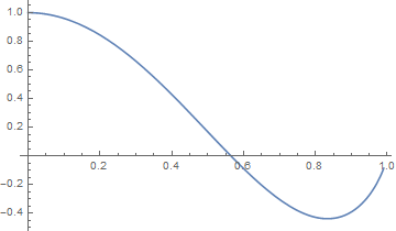
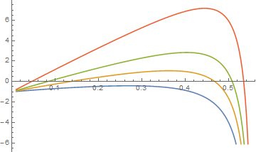
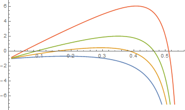
Figure 1: Left: The function $P(y)$. The plot shows the range of acceptable values of $y$. Middle: $a(y)$ for $x_{0}=0.3,\ 0.4,\ 0.5,\ 0.75$ (upside down). Right: $a(y)+c(y)$ for $x_{0}=0.3,\ 0.4,\ 0.5,\ 0.75$ (upside down). The data for $x_{0}=0.75$ are included to show that larger $x_{0}$ values inevitably lead to WEC violation.

This reasoning, beginning with (30), is of quite a general nature for any surfaces $x={\rm const}$ in space-times with the metric (2). Let us now specify the matrix elements $a,b,c,d$ for the surfaces $\Sigma_{\pm}$ in our particular construction, assuming for certainty $\omega_{0}>0$ in the internal solution and $\Omega>0$ in ${\mathbb{M}}_{+}$.

Consider $\Sigma_{+}$, hence for any $f$ we write $[f]=f_{\rm out}-f_{\rm in}$, where $f_{\rm out}$ is taken from the region ${\mathbb{M}}_{+}$ with the metric (20) at $X=r_{0}$, and $f_{\rm in}$ from the wormhole solution (2)–(18) at $x=x_{+}$. Taking into account the junction conditions (27)–(29), we obtain (ignoring the insignificant common factor $1/r_{0}$):

$${}a=-\frac{1}{P(y)}+\frac{M(y)}{x_{0}^{2}}\bigg{(}\frac{y}{1-y^{2}}+{{\displaystyle\frac{1}{2}}}L(y)\bigg{)},$$

$${}b=1,$$

$${}c=-\frac{1}{P(y)}+1+\frac{M(y)}{x_{0}^{2}}\bigg{(}\frac{y}{1-y^{2}}-{{\displaystyle\frac{1}{2}}}L(y)\bigg{)},$$ (39)

$${}d=-\frac{\sqrt{1-P(y)}}{P(y)}+\frac{M(y)}{x_{0}^{2}(1-y^{2})},$$ (40)

where we use the notations

$${}y=\frac{x_{+}}{x_{0}},\hskip 28.45274ptL(y)=\ln\frac{1+y}{1-y},$$

$${}M(y)=\big{(}1-y\big{)}^{-(1-y)/2}\big{(}1+y\big{)}^{-(1+y)/2},$$ (41)

and for the quantity $P$ defined in (28) we have

$$P(y)=(1-y^{2})\Big{[}1-yL(y)-\frac{1}{4}(1-y^{2})L^{2}(y)\Big{]}.$$ (42)

The expressions for $a,b,c$ depend on two parameters, $x_{0}$ and $y$, and, by symmetry of our construction, they are the same on both $\Sigma_{+}$ and $\Sigma_{-}$. Unlike that, when calculating $d=-[\omega]$ for $\Sigma_{-}$, we should take into account different signs of $\Omega$ on the two junctions. As a result, on $\Sigma_{-}$ in the expression (40) for $[d]$ there are minuses at both terms (whose own values are the same as in (40)), and so the absolute value of $[d]$ is larger than on $\Sigma_{+}$. However, in our WEC analysis, the particular value of $d=-[\omega]$ is not important since, as follows from (36)–(38), the WEC fulfillment only depends on $a$ and $c$ if $b\geq 0$, and in our case $b=1$.

In Eqs. (3)–(42) all quantities are dimensionless, and one can verify the following (see Fig. 1):

$\bullet$ The condition $0<P(y)<1$, necessary for all the above expressions to make sense, holds for $0<|y|<0.564)$ (this and further numerical estimates are approximate). One can notice that the admissible range of $y$ is the same as was previously found for the absence of CTCs. This is not surprising since $g_{33}$ on $\Sigma_{\pm}$ is common for the internal and external regions, and the latter, being flat, is manifestly free of CTCs. Since $|y|$ in the internal region is smaller than on $\Sigma_{\pm}$, this region is also CTC-free.

$\bullet$ The condition $a>0$ (equivalent to $\sigma>0$ in the noncomoving reference frame on $\Sigma_{\pm}$ in which the junction conditions were written) holds, in particular, for $x_{0}=0.5,\ y\in(0.15,0.47)$ and for $x_{0}=0.3,\ y\in(0.05,0.53)$.

$\bullet$ The condition $a>c$, necessary for interpreting the roots as shown in (3), holds practically in the same ranges of $y$ for $x_{0}$ (at least) between 0.3 and 0.5.

$\bullet$ The condition $a+c>0$ also holds in a sufficiently large range of the parameters, e.g, for $x_{0}=0.5,\ y\in(0.15,0.38)$ and for $x_{0}=0.3,\ y\in(0.05,0.51)$.

Since the conditions (36) and (37) manifestly hold if (38) does, we conclude that there is a significant range in the parameter space ($x_{0},y$) in which our wormhole model completely satisfies the WEC.

4 Concluding remarks

Using an explicit example of an anisotropic fluid as a source of gravity, we have achieved our goal and demonstrated the possibility of obtaining a regular, radially asymptotically flat traversable cylindrical wormhole in GR.

There is, however, a subtle point that may put to doubt the consistency of the whole construction. The present model contains thin shells on two surfaces and is consistent in the framework of the thin shell formalism. However, if a thin shell is physically understood as some approximation to a smooth thick layer with matter content rapidly varying in a region of finite extent, there emerges a discrepancy with the shell (here, $\Sigma_{-}$) that separates the internal region with $\omega_{0}>0$ with the external one where $\Omega=\Omega_{-}<0$. For a smooth, differentially rotating matter in a thick shell, one can define a comoving frame in which Eq. (3) should hold everywhere with fixed $\omega_{0}>0$. It is then hard to understand how it can be smoothly joined to the outside $\Omega<0$.

A possible answer is to recall that in vacuum (hence in the region ${\mathbb{M}}_{-}$) any reference frame is comoving. Therefore we can imagine that the layer of matter with $\omega>0$ is smoothly matched to a reference frame in ${\mathbb{M}}_{-}$ with $\Omega>0$, but for the description of the whole configuration we are using there a frame in which $\Omega=\Omega_{-}<0$. Technically, this corresponds to a rapid change of $\Omega=\Omega(x)$ in a vacuum layer close to the matter distribution replacing the thin shell.

Or, as an alternative, we may assume that in this thin but finite layer of matter there is a still thinner (but also finite) intermediate vacuum layer ${\mathbb{M}}_{\rm int}$. Then nothing prevents us to use one reference frame in ${\mathbb{M}}_{\rm int}$ for matching it to the matter layers on the “positive” side with $\omega>0$ and another one for matching to the “negative” side with $\omega<0$ that will in turn smoothly join the vacuum region ${\mathbb{M}}_{-}$.

This reasoning, though apparently correct, still looks rather artificial, and it would be more preferable to obtain a model in which both $\Omega({\mathbb{M}}_{\pm})>0$. It can be shown, however, that at least with the present internal solution (2)–(18) such a model cannot be obtained, see the Appendix. We can hope that other sources of gravity in the internal region can provide such a model.

Appendix

Let us try to modify the model built in Section 3 by assuming $E_{0}>0$, so that it could be matched to both $\Omega({\mathbb{M}}_{\pm})>0$. As before, we assume $\omega_{0}>0$ and use the notations $y=x/x_{0}$. For $E(x)$ we can write

$$E=\frac{r_{0}(1-y^{2})}{2}\bigg{[}\frac{2y}{1-y^{2}}+\ln\frac{1+y}{1-y}+E_{0}\bigg{]}.$$ (A.1)

The matching conditions on $\Sigma_{\pm}$ have the same form (22). The condition $[\mu]=0$ does not affect our consideration. The conditions $[\gamma]=0$ and $[\beta]=0$, as before, lead to

$${}Q^{2}x_{0}^{2}(1-y_{\pm}^{2})=1-\Omega^{2}X_{\pm}^{2}=:P_{\pm},$$ (A.2)

$${}\frac{r_{0}^{2}}{Q^{2}x_{0}^{2}(1-y_{\pm}^{2})}=\frac{X_{\pm}^{2}}{1-\Omega^{2}X_{\pm}^{2}}.$$ (A.3)

From (A.2), (A.3) it follows $X_{\pm}^{2}=r_{0}^{2}$. Furthermore, the condition $[E]=0$ yields, instead of (42),

$${}P(y)=(1-y^{2})\Big{[}1-(L+E_{0})$$

$${}\hskip 72.26999pt-\frac{(1-y^{2})}{4}(L+E_{0})^{2}\Big{]},$$ (A.4)

where we have omitted the index $\pm$ near $P$ and $y$, and, as before, $L=\ln\dfrac{1+y}{1-y}$.

Our task is to find, instead of $y_{-}=-y_{+}$, such values of $y_{\pm}$ for the surfaces $\Sigma_{\pm}$ that

1. $y_{+}>0$ and $y_{-}<0$ (to provide the wormhole nature of the internal region where $y=0$ is the throat);

2. Both $E(y_{\pm})>0$, to be matched with $E=\Omega r_{0}^{2}$ and to provide $\Omega>0$ in ${\mathbb{M}}_{\pm}$

Figure 2: The function $H(y,E_{0})$

From (A.2) it follows that the function

$$H(y,E_{0}):=P(y)/(1-y^{2})$$

takes the same value equal to $Q^{2}x_{0}^{2}$ on both junctions, that is, $H(y_{+})=H(y_{-})$. As a function of $y$, $H$ has a single $E_{0}$-dependent maximum (see Fig. 2), hence $y_{+}$ and $y_{-}$ are located on different sides of this maximum.

On the other hand, $E(y)$ given by (A.1) is a monotonically growing function and takes a zero value at the point $y=y_{*}<0$ where $L+E_{0}=-2y/(1-y^{2})$. By Requirement 2, both $y_{\pm}$ should be located on the $y$ axis to the right of $y_{*}$. However, it is straightforward to verify that, at any fixed $E_{0}$, $dH/dy(y_{*})<0$, that is, this point is located on the descending part of the plot of $H(y)$, to the right of its maximum, hence only $y_{+}$ can be larger than $y_{*}$, and Requirement 2 cannot be fulfilled.

We see that the present solution cannot lead to a model with $E(y_{\pm})>0$.

Acknowledgments

This publication was supported by the RUDN University program 5-100. The work of KB was performed within the framework of the Center FRPP supported by MEPhI Academic Excellence Project (contract No. 02.a03.21.0005, 27.08.2013) and by Russian Basic Research Foundation Grant 19-02-00346. The work of VK was supported by the Ministry of Education and Science of Russia in the framework of State Contract 9.1195.2017.6/7.

References

- [1] A. Doroshkevich, J. Hansen, I. Novikov, and A. Shatskiy, Passage of radiation through wormholes. Int. J. Mod. Phys. D 18, 1665 (2009); arXiv: 0812.0702.
- [2] T. Harko, Z. Kovacs, and F. S. N. Lobo, Thin accretion disks in stationary axisymmetric wormhole spacetimes. Phys. Rev. D 79, 064001 (2009); arXiv: 0901.3926.
- [3] A. A. Kirillov and E. P. Savelova, On the value of the cosmological constant in a gas of virtual wormholes Grav. Cosmol. 19, 92 (2013).
- [4] K. A. Bronnikov and K. A. Baleevskikh, On gravitational lensing by symmetric and asymmetric wormholes. Grav. Cosmol. 25, 44 (2019); arXiv: 1812.05704.
- [5] M. Morris, K.S. Thorne, and U. Yurtsever, Wormholes, time machines, and the Weak Energy Condition. Phys. Rev. Lett. 61, 1446 (1988).
- [6] M. Visser, Lorentzian Wormholes: from Einstein to Hawking (AIP, Woodbury, 1995).
- [7] D. Hochberg and M. Visser, Geometric structure of the generic static traversable wormhole throat, Phys. Rev. D 56, 4745 (1997); gr-qc/9704082.
- [8] K. A. Bronnikov and S. G. Rubin, Black Holes, Cosmology and Extra Dimensions (World Scientific, Singapore, 2012).
- [9] J. L. Friedman, K. Schleich, and D. M. Witt, Topological censorship. Phys. Rev. Lett. 71, 1486-1489 (1993); Erratum: ibid. 75, 1872 (1995).
- [10] G. J. Galloway, On the topology of the domain of outer communication Class. Quantum Grav. 12, L99 (1995).
- [11] J. L. Friedman and A. Higuchi, Topological censorship and chronology protection. Ann. Phys. 15, 109-128 (2006); arXiv: 0801.0735.
- [12] K. A. Bronnikov and A. M. Galiakhmetov, Wormholes without exotic matter in Einstein-Cartan theory, Grav. Cosmol. 21, 283 (2015); arXiv: 1508.01114.
- [13] K. A. Bronnikov and A. M. Galiakhmetov, Wormholes without exotic matter in Einstein-Cartan theory, Phys. Rev. D 94, 124006 (2016); arXiv: 1607.07791.
- [14] H. Maeda and M. Nozawa, Static and symmetric wormholes respecting energy conditions in Einstein-Gauss-Bonnet gravity. Phys. Rev. D 78, 024005 (2008).
- [15] K. A. Bronnikov and S.-W. Kim, Possible wormholes in a brane world. Phys. Rev. D 67, 064027 (2003); gr-qc/0212112)
- [16] K. A. Bronnikov and M. V. Skvortsova, Wormholes leading to extra dimensions Grav. Cosmol. 22, 316 (2016).
- [17] D. Zipoy, Topology of some spheroidal metrics. J. Math. Phys. 7, 1137 (1966).
- [18] K. A. Bronnikov and J. C. Fabris, Weyl spacetimes and wormholes in -dimensional Einstein and dilaton gravity Class. Quantum Grav. 14, 831 (1997); gr-qc/9603037.
- [19] G. Miranda and T. Matos, Exact rotating magnetic traversable wormholes satisfying the energy conditions arXiv: 1507.02348.
- [20] E. Ayón-Beato, F. Canfora, and J. Zanelli, Analytic self-gravitating Skyrmions, cosmological bounces and AdS wormholes Phys. Lett. B 752, 201 (2016).
- [21] F. Canfora, N. Dimakis, and A. Paliathanasis, Topologically nontrivial configurations in the 4d Einstein?nonlinear -model system Phys. Rev. D 96, 025021 (2017).
- [22] F. Schein and P. C. Aichelburg, Traversable wormholes in geometries of charged shells Phys. Rev. Lett. bf 77, 4130 (1996).
- [23] K. A. Bronnikov and José P. S. Lemos, Cylindrical wormholes. Phys. Rev. D 79, 104019 (2009); arXiv: 0902.2360.
- [24] K. A. Bronnikov, V. G. Krechet, and José P. S. Lemos, Rotating cylindrical wormholes. Phys. Rev. D 87, 084060 (2013); arXiv: 1303.2993.
- [25] K. A. Bronnikov and V. G. Krechet, Rotating cylindrical wormholes and energy conditions, Int. J. Mod. Phys. A 31, 1641022 (2016); arXiv: 1509.04665.
- [26] K. A. Bronnikov, Rotating cylindrical wormholes: A no-go theorem. J. Phys. Conf. Series 675, 012028 (2016); arXiv: 1509.06924.
- [27] K. A. Bronnikov and M. V. Skvortsova, Cylindrically and axially symmetric wormholes. Throats in vacuum? Grav. Cosmol. 20, 171 (2014); arXiv: 1404.5750.
- [28] T. Levi-Civita, einsteiniani in campi newtoniani. IX: L’analogo del potenziale logaritmico. Rend. Accad. Lincei, 28, 101 (1919).
- [29] T. Lewis, ‘Some special solutions of the equations of axially symmetric gravitational fields.” Proc. R. Soc. A 136, 176 (1932).
- [30] H. Stephani, D. Kramer, M.A.H. MacCallum, C. Hoenselaers, and E. Herlt, Exact Solutions of Einsteins Field Equations, Cambridge Monographs on Mathematical Physics (Cambridge University Press, 2009).
- [31] A. Vilenkin and E P. S. Shellard, Cosmic Strings and Other Topological Defects (Cambridge Univ. Press, Cambridge, 1994).
- [32] V. G. Krechet, Topological and physical effects of rotation and spin in the general relativistic theory of gravitation. Russ, Phys, J. 50, 1021 (2007); Izvestiya Vuzov, Fiz. No.10, 57 (2007).
- [33] V. G. Krechet and D. V. Sadovnikov, Spin-spin interaction in general relativity and induced geometries with nontrivial topology. Grav. Cosmol. 15, 337 (2009); arXiv: 0912.2181.
- [34] W. Israel, Singular hypersurfaces and thin shells in general relativity. Nuovo Cim. B 48 463 (1967).
- [35] V. A. Berezin, V. A. Kuzmin, and I. I. Tkachev, Dynamics of bubbles in general relativity. Phys. Rev. D 36, 2919 (1987).
- [36] F. Debbasch, L. Herrera, P. R. C. T. Pereira, and N. O. Santos, Stationary cylindrical anisotropic fluid. Gen. Rel. Grav. 38, 1825 (2006); gr-qc/0609068.
- [37] Ø. Grøn and S. Johannesen, Closed timelike geodesics in a gas of cosmic strings. New J. Phys. 10, 103025 (2008); gr-qc/0703139.