Surface gravities for 15,000 Kepler stars measured from stellar granulation and validated with Gaia DR2 parallaxes

Abstract

We have developed a method to estimate surface gravity ($\log g$) from light curves by measuring the granulation background, similar to the “flicker” method by Bastien et al. (2016) but working in the Fourier power spectrum. We calibrated the method using Kepler stars for which asteroseismology has been possible with short-cadence data, demonstrating a precision in $\log g$ of about 0.05 dex. We also derived a correction for white noise as a function of Kepler magnitude by measuring white noise directly from observations. We then applied the method to the same sample of long-cadence stars as Bastien et al. We found that about half the stars are too faint for the granulation background to be reliably detected above the white noise. We provide a catalogue of $\log g$ values for about 15,000 stars having uncertainties better than 0.5 dex. We used Gaia DR2 parallaxes to validate that granulation is a powerful method to measure $\log g$ from light curves. Our method can also be applied to the large number of light curves collected by K2 and TESS.

1 Introduction

The surface gravity of a star is one of its most fundamental parameters. It is of particular interest for stars hosting transiting exoplanets, due to its direct dependence on the stellar (and hence planetary) radius. Traditionally, $\log g$ is estimated from high-resolution spectra by measuring pressure broadening of absorption lines or using ionization equilibrium, but these approaches are often plagued by degeneracies with other atmospheric parameters such as temperature and metallicity (Torres et al., 2012). Asteroseismology using data from the Kepler Mission (Borucki et al., 2010) has been demonstrated to provide accurate surface gravities for the brighter FGK stars (Chaplin et al., 2014; Serenelli et al., 2017). For red giants, which oscillate at relatively low frequencies, observations in long-cadence mode (29.4 minutes) can be used (e.g., Yu et al., 2018). However, measuring oscillations in main-sequence and subgiant stars requires short-cadence observations (58.9 s), which were only obtained for a small fraction of Kepler stars. For those tens of thousands of Kepler stars that were only observed in long-cadence mode, which includes the majority of stars hosting transiting planet candidates, it is still possible to infer $\log g$ by measuring the low-frequency photometric fluctuations from granulation (Mathur et al., 2011a; Bastien et al., 2013; Cranmer et al., 2014; Kallinger et al., 2016a; Bugnet et al., 2017; Ness et al., 2018). For example, Bastien et al. (2016, hereafter B16) measured granulation in the time series using a fixed 8-hour filter, which they referred to as “flicker" ($F_{8}$), deriving $\log g$ for nearly 28,000 stars with a typical precision of about 0.1 dex. Somewhat controversially, flicker results implied that nearly 50% of all bright exoplanet host stars are subgiants, resulting in 20%–30% larger planet radii than previous measurements had suggested (Bastien et al., 2014). However, radius estimates using the recently-released Gaia DR2 parallaxes imply an upper limit on the subgiant fraction of $\sim$ 23% (Berger et al., 2018).

A common approach for previous methods using long-cadence data is to measure granulation power over a fixed frequency range, either in the time domain (B16) or in the frequency domain (Bugnet et al., 2017). Here, we present a new method that adapts to the fact that the granulation timescale shifts in frequency depending on the evolutionary state of the star (Kjeldsen & Bedding, 2011a). Additionally, our method is able to provide reliable $\log g$ uncertainties, thus allowing a quantitative estimate of whether granulation has been reliably detected in each star. Both of these developments will be critical to applying granulation-based $\log g$ estimators to the large number of stars expected to be observed with the TESS mission.

2 Method

2.1 Surface gravities from photometric time series

For stars in which solar-like oscillations can be measured, it is now quite well-established that the frequency of maximum oscillation power, $\nu_{\rm max}$, scales in a simple way with surface gravity and effective temperature (Brown et al., 1991; Kjeldsen & Bedding, 1995):

$$\mbox{$\nu_{\rm max}$}\propto g/\sqrt{\mbox{$T_{\rm eff}$}}.$$ (1)

Using this scaling relation, $\log g$ can be measured from asteroseismology with an accuracy of about 0.03 dex for main-sequence stars, based on comparisons with oscillating stars in binary systems (Miglio, 2012; Huber, 2015).

In stars where oscillations cannot be sampled directly because short-cadence data are not available, we can estimate $\log g$ by measuring the slow variations from granulation. The strength of these variations correlates directly with $\nu_{\rm max}$ (Kjeldsen & Bedding, 2011b; Chaplin et al., 2011; Mathur et al., 2011b; Hekker et al., 2012; Samadi et al., 2013; Kallinger et al., 2014; Bugnet et al., 2017; de Assis Peralta et al., 2018; Yu et al., 2018), and can therefore provide a way to infer $\log g$ (provided $T_{\rm eff}$ is known). This correlation arises because the same underlying mechanism, namely convection, is responsible for both the oscillations and the granulation. Note that the photometric variations from granulation behave like $1/f$ noise in that they depend on the timescale on which they are measured. In the Fourier power spectrum, this is seen as a background that rises towards low frequencies (see the example in Fig. 1).

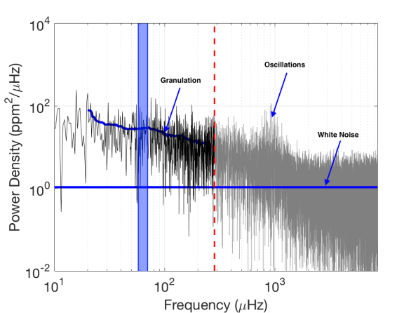
Figure 1: Power spectrum of a bright main-sequence star observed by Kepler in short-cadence mode. The star is KIC 6370489 and the power spectrum is based on data from Q1. We see a power excess from solar-like oscillations at $\mbox{$\nu_{\rm max}$}=914\,\mbox{$\mu$Hz}$, a granulation background that rises towards lower frequencies, and a flat background from white noise. The red dashed line indicates the Nyquist frequency for long-cadence observations ($283\mbox{$\mu$Hz}$). The blue strip marks a passband centred at $0.08\mbox{$\nu_{\rm max}$}$ with fractional bandwidth 20%.

2.2 Short-cadence benchmark sample

As a first step, we established an empirical relationship between granulation power, $P_{\rm gran}$, and the frequency of maximum oscillation power, $\nu_{\rm max}$. To do this, we used the same benchmark sample of 542 Kepler stars from Huber et al. (2011) that was used by Bastien et al. (2013) to calibrate their relation. These stars have $\nu_{\rm max}$ measurements from short-cadence data, with uncertainties derived as described by Huber et al. (2011). We analysed the long-cadence data for these stars, as follows:

1. we downloaded Simple Aperture Photometry (SAP) from MAST for all available quarters, and treated each quarter separately;

2. we removed points affected by spacecraft safe-mode events, those with quality flag $>0$, and those with contamination flags $<0.95$;

3. we clipped outliers that were more than 4 standard deviations away from the local mean, where the latter was calculated over a 90-minute moving window;

4. we applied a high-pass filter (Savitzky & Golay, 1964) to remove very slow variations arising from stellar activity, instrumental noise and other sources, which could otherwise leak to higher frequencies. We adapted this filter to each star (see also Kallinger et al., 2016b), with the cut-off set to eliminate power at frequencies below $0.02\mbox{$\nu_{\rm max}$}$.

5. we calculated the Fourier power spectrum for each quarter up to the long-cadence Nyquist frequency ($284\mbox{$\mu$Hz}$). We multiplied by the total duration of the observations in order to convert to power density (in ${\rm ppm}^{2}/\mbox{$\mu$Hz}$), allowing us to measure the granulation background and the white noise level (e.g., Kjeldsen et al., 1999).

6. we measured the granulation background in the power density spectrum in a bandpass with fractional width 20% centred at $0.08\mbox{$\nu_{\rm max}$}$, as shown in Fig. 1. Our choice of parameters for this bandpass is explained in Sec. 2.5.

We measured the granulation power for each star in this way for every quarter of Kepler data (except Q0, the first ten days of observation). We took the median of these measurements as our estimate of the granulation power and the standard deviation over all quarters as its uncertainty. From this measured granulation power we subtracted the appropriate white noise correction, as described in the next section.

2.3 White-noise correction

The Kepler light curves include Poisson noise from photon-counting statistics. In the Fourier transform this appears as a frequency-independent (flat) noise that is greater for fainter stars. It is important to correct for this white noise, since otherwise the granulation power will be overestimated.

Measuring the white noise directly requires access to high frequencies, which is only possible with short-cadence data (see Fig. 1). We have used a sample of $\sim$2100 stars for which short-cadence observations are available to construct a calibration curve of white noise as a function of Kepler magnitude, Kp (see also Gilliland et al., 2010). This is a much larger group of stars than the benchmark sample introduced in Sec. 2.2 and includes many, especially at the faint end, for which oscillations were not detected. We calculated Fourier spectra for individual quarters of Kepler data, as described in Sec. 2.2, and measured the average power density in the region 6000–8000 $\mu$Hz. This is above the range of oscillation frequencies in all stars and so provides a good estimate of the white noise.

Figure 2: Calibration of white noise level as a function of Kepler magnitude. The grey points are measurements from power density spectra of $\sim$2100 stars observed in short-cadence mode. The black points and error bars show the median and scatter of points in bins of width 0.6 mag. The blue line connects these points into a piecewise-linear calibration curve.

The measurements of white noise are shown in Fig. 2. Most of the stars are bright ($\mbox{Kp}<12$) but there are enough fainter stars to define the white-noise level accurately down to $\mbox{Kp}=16$. Our calibration curve as a function of Kp (blue line) is based on the medians in bins of width 0.6 magnitudes. The error bars show the uncertainties on the correction, which are calculated as the median absolute deviation within each bin. We subtracted this white-noise level from the granulation power measured for each star in the benchmark sample (Sec. 2.2), and also for the main sample (Sec. 3.1). The uncertainty in the white noise correction was added in quadrature to the quarter-to-quarter uncertainty estimate of granulation power described in the next section.

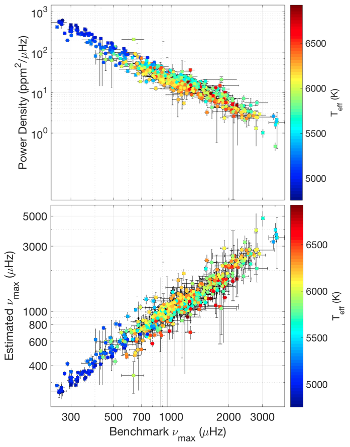
Figure 3: Granulation power (upper) and the inferred value of $\nu_{\rm max}$ using Eq. 2 (lower) for the benchmark sample, plotted against $\nu_{\rm max}$ measured by Huber et al. (2011) from short-cadence data. Colour represents $T_{\rm eff}$ (Mathur et al., 2017).

2.4 Calibrating the relation

The upper panel of Fig. 3 shows our measured granulation power density, $P_{\rm gran}$, for each star in the benchmark sample after correcting for white noise. These values are plotted against $\nu_{\rm max}$ for each star, as measured by Huber et al. (2011) from the oscillations themselves using short-cadence data. We confirm the strong correlation that was previously found from Kepler data (Chaplin et al., 2011; Huber et al., 2011; Samadi et al., 2013; Kallinger et al., 2014). However, we also see a clear dependence on effective temperature, indicating that we should include $T_{\rm eff}$ in our fit.

We calculated the fit as a linear function relating $\log\mbox{$\nu_{\rm max}$}$, $T_{\rm eff}$ and $\log\mbox{$P_{\rm gran}$}$ as follows:

$$\begin{split}\log(\mbox{$\nu_{\rm max}$}/\mbox{$\mu$Hz})=-0.4861\log(\mbox{$P_{\rm gran}$}/({\rm ppm}^{2}/\mbox{$\mu$Hz}))-\\ \mbox{$T_{\rm eff}$}/(11022\,{\rm K})+4.197.\end{split}$$ (2)

The lower panel of Fig. 3 shows the relation between $\nu_{\rm max}$ estimated from this fit and the measured benchmark values. The comparison show good agreement, with systematic variations below the 5% level. Converting $\nu_{\rm max}$ to $\log g$ via Eq. 1 gives $\log g$ values for the benchmark sample with a scatter of $\sim$0.05  dex.

2.5 Determining the bandpass

As noted in Sec. 2.2, we measured the granulation background in the power spectrum of each star adaptively at a fixed fraction of $\nu_{\rm max}$. The frequency of this bandpass should be low enough that it falls below the long-cadence Nyquist frequency for all stars of interest, and high enough that it is unaffected by the high-pass filter described in Sec. 2.2. We tested bandpasses with centres in the range from $0.04\mbox{$\nu_{\rm max}$}$ to $0.10\mbox{$\nu_{\rm max}$}$. We also tested different values for the fractional width of the bandpass, from 10% to 50%.

In order to choose the optimal bandpass, we sought to minimize the scatter between our derived values of $\nu_{\rm max}$ and those measured by Huber et al. (2011), as plotted in the lower panel of Fig. 3. At the same time, we also aimed to avoid excluding stars for which this bandpass would lie above the Nyquist frequency for long-cadence data. We settled on a bandpass with fractional width 20% centred at $0.08\mbox{$\nu_{\rm max}$}$, as shown in Fig. 1.

3 Results and Discussion

3.1 The catalogue of surface gravities

We applied our method to measure $\log g$ for the same sample of long-cadence stars that was analysed by B16. This comprises 28,715 stars with $\mbox{Kp}\ <13.5$, the majority of which have $\mbox{Kp}>12$. We excluded 262 stars that are listed in the Kepler Eclipsing Binary Catalog by Kirk et al. (2016), since the eclipses have harmonics in the power spectrum that interfere with measuring the granulation background.

Our method requires knowledge of $\nu_{\rm max}$ in order to carry out the high-pass filtering and also to set the bandpass in which $P_{\rm gran}$ is measured (Sec. 2.2). We therefore adopted an iterative approach, with the initial estimate of $\nu_{\rm max}$ being calculated from values of $\log g$ and $T_{\rm eff}$ in the Kepler Input Catalog (KIC) (Brown et al., 2011). In practice, we found that the choice of this initial $\nu_{\rm max}$ did not significantly affect the final result in most cases.

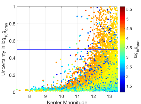
Figure 4: The uncertainty in our $\log g$ estimates plotted against Kp. Colour represents our $\log g$ estimates. The horizontal blue line shows the cut we made at an uncertainty of 0.5 dex.

For 4181 giants with $\mbox{$\nu_{\rm max}$}<100\,\mbox{$\mu$Hz}$, the process did not converge after three iterations and those stars were excluded from the sample. For a further 818 stars, mostly cool dwarfs, the granulation power was too close to the white noise level to be measured. The remaining sample contained 23454 stars. Figure 4 shows their $\log g$ uncertainties as a function of Kepler magnitude. We see that many have large uncertainties, mainly faint dwarfs, indicating the difficulty of measuring their granulation signal above the white noise. Our final catalogue, for which estimates of $P_{\rm gran}$, $\nu_{\rm max}$ and $\log g$ are listed in Table 1, comprises 15109 stars having uncertainties in $\log g$ smaller than 0.5 dex.

Table 1: Estimates of granulation power, $\nu_{\rm max}$ and $\log g$ for 15,109 stars using Kepler long-cadence data. Effective temperatures are taken from Mathur et al. (2017). (This table is available in its entirety in a machine-readable form in the online journal. A portion is shown here for guidance regarding its form and content.)

KIC	Kp	$T_{\rm eff}$ (K)	$P_{\rm gran}$ (${\rm ppm}^{2}/\mbox{$\mu$Hz}$)	$\nu_{\rm max}$ ($\mu$Hz)	$\log g$
1025494	11.822	6122(172)	32.20(5.12)	810.7(91.8)	3.87(0.05)
1026084	12.136	5072(166)	21357.21(3217.25)	42.9(4.6)	2.55(0.05)
1026255	12.509	7050(214)	151.11(17.57)	315.0(31.9)	3.49(0.04)
1026475	11.872	6611(189)	18.78(6.18)	951.3(189.8)	3.96(0.09)
1026669	12.304	6293(193)	21.24(9.15)	957.6(239.0)	3.95(0.11)

It is worth noting that the granulation power in red giants has a slight metallicity dependence, in the sense that metal-rich stars have stronger granulation (Corsaro et al., 2017; Yu et al., 2018). If such a relation applied to the main-sequence and subgiant stars studied here, it would affect the values of $\log g$ derived from measuring granulation power.

3.2 Comparison with Spectroscopy

We compared our estimates with those obtained from spectroscopy in Fig. 5. We adopted spectroscopic parameters for 3017 stars from the Kepler Stellar Properties Catalog (Mathur et al., 2017), which primarily contains values from LAMOST (2075 sources, Luo et al., 2015; De Cat et al., 2015), APOGEE (588 sources, Alam et al., 2015) and Buchhave et al. (2014). The comparison generally shows good agreement and no trend with Kp but there is a small systematic offset of $\sim$0.05 dex.

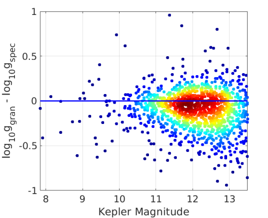
Figure 5: Difference in $\log g$ between our estimates and those from spectroscopy, plotted against Kp. Colours represents the density of stars in each region.

Spectroscopic estimates of $\log g$ should generally be unaffected by distance or interstellar reddening. On the other hand, estimating $\log g$ from photometric fluctuations is potentially very sensitive to the way that white photon noise is accounted for. Therefore, the fact that we do not see a systematic trend with Kp in Fig. 5 gives us confidence that our white-noise correction is effective. For comparison, such a trend is seen in Fig. 1 of Bastien et al. (2014).

3.3 Comparison with Gaia Parallaxes

The recent release of Gaia DR2 parallaxes (Gaia Collaboration et al., 2018; Lindegren et al., 2018) provides another opportunity to test our $\log g$ values and to validate granulation-based surface gravities with a larger sample than the benchmark asteroseismic detections from Kepler short-cadence data. To do this, we combined the $\log g$ values from Table 1 with effective temperatures and metallicities from Mathur et al. (2017) to calculate luminosities from isochrones using the software package isoclassify (Huber et al., 2017). We restricted the analysis to the $\sim$ 13,400 stars in our sample with $\log g$ uncertainties below 0.3 dex.

The left panel of Fig. 6 compares our luminosities to those derived from Gaia parallaxes by Berger et al. (2018). We see good agreement over three orders of magnitude, but a systematic discrepancy for high-luminosity red giants ($\gtrsim 100\,L_{\odot}$, $\mbox{$\log g$}<2.3$), for which our $\log g$ values are systematically too small. We suspect that this difference is due to the extrapolation of our calibration, which is mostly based on main-sequence stars and subgiants (Fig. 3). Excluding these high-luminosity giants, we find a residual scatter of 40%, which is roughly consistent with the typical uncertainties on the granulation-derived luminosities (which includes uncertainties on $T_{\rm eff}$, $\log g$ and $\rm{[Fe/H]}$). Systematic differences are at the level of 7% or less in luminosity, which corresponds to $\sim$ 0.07 dex in $\log g$. However, we note that systematic errors in the $T_{\rm eff}$ scale may account for part of this. The right panel of Figure 6 shows the same comparison but using flicker-derived $\log g$ values from B16. As expected, the overall performance of flicker-derived $\log g$ values is similar to ours, with a slightly higher scatter and different systematics for high-luminosity giants.

Overall, this comparison with Gaia validates granulation as a powerful tool to measure $\log g$ from light curves with good precision. Combined with radii from Gaia parallaxes, this may allow the measurement of masses for a large number of individual stars without using stellar models (Stassun et al., 2018). However, we caution that systematic differences at the $<0.1$ dex level due to uncertainties in the $\nu_{\rm max}$ scaling relations and white noise corrections still need to be carefully quantified.

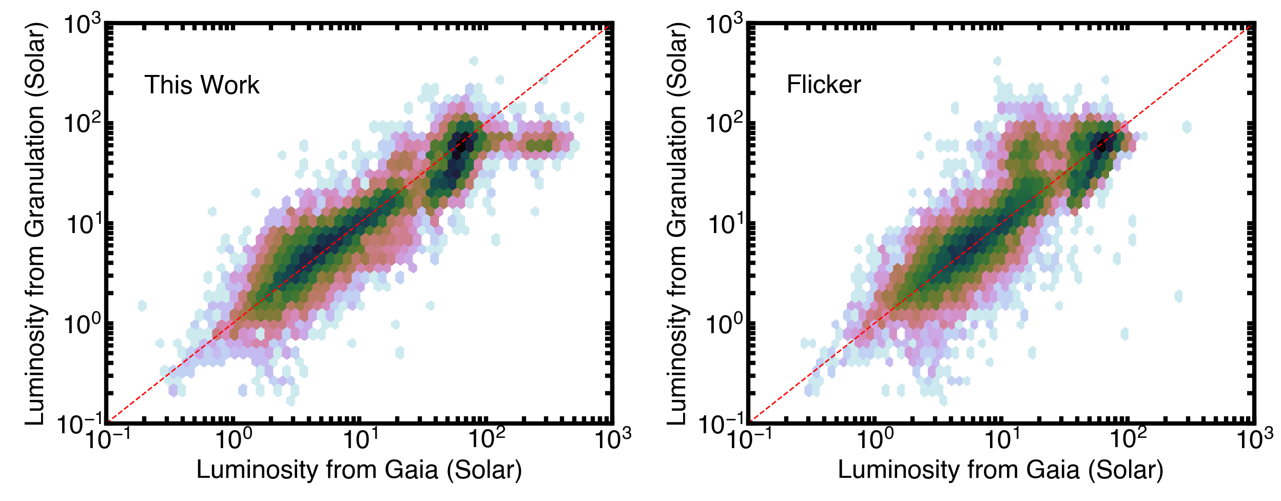
Figure 6: Comparison of luminosities derived from Gaia DR2 parallaxes from Berger et al. (2018) with luminosities derived the granulation-based $\log g$ values in our work (left panel) and $\log g$ values from flicker (right panel, B16). Only stars with $\log g$ values measured to better than 0.3 dex with our method are shown in both panels. Colors show logarithmic number density, and the red line marks equality.

4 Conclusion

We have estimated $\log g$ from Kepler light curves by measuring the granulation background, similar to the “flicker” method by Bastien et al. (2016) but working in the Fourier power spectrum. We established a calibration for white noise as a function of magnitude (Fig. 2) and calibrated the granulation power using the asteroseismic short-cadence sample, demonstrating a precision in $\log g$ of about 0.05 dex (Fig. 2.2). Applying the method to the sample of 28,000 long-cadence stars studied by Bastien et al. (2016), we found about half the stars to be too faint for the granulation background to be reliably detected above the white noise. We have provided an electronic catalogue of $\log g$ values (with uncertainties) for about 15,000 stars having $\log g$ uncertainties better than 0.5 dex (Table 1).

There is no magnitude-dependent trend in the difference between our estimates and those available from spectroscopy, giving us confidence that our white noise correction is effective. We also use Gaia DR2 parallaxes to validate that granulation is a powerful method to measure $\log g$ from light curves. Our method can also be applied to the large number of light curves collected by K2 and TESS.

References

- Alam et al. (2015) Alam S., et al., 2015, ApJS, 219, 12
- Bastien et al. (2013) Bastien F. A., Stassun K. G., Basri G., Pepper J., 2013, Nature, 500, 427
- Bastien et al. (2014) Bastien F. A., Stassun K. G., Pepper J., 2014, ApJ, 788, L9
- Bastien et al. (2016) Bastien F. A., Stassun K. G., Basri G., Pepper J., 2016, ApJ, 818, 43
- Berger et al. (2018) Berger T. A., Huber D., Gaidos E., van Saders J. L., 2018, preprint, (arXiv:1805.00231)
- Borucki et al. (2010) Borucki W. J., et al., 2010, Science, 327
- Brown et al. (1991) Brown T. M., Gilliland R. L., Noyes R. W., Ramsey L. W., 1991, ApJ, 368, 599
- Brown et al. (2011) Brown T. M. T., Latham D. W. D., Everett M. E. M., Esquerdo G. A. G., 2011, AJ, 142, 112
- Buchhave et al. (2014) Buchhave L. A., et al., 2014, Nature, 509, 593
- Bugnet et al. (2017) Bugnet L., García R. A., Davies G. R., Mathur S., Corsaro E., 2017, in Reylé C., Di Matteo P., Herpin F., Lagadec E., Lançon A., Meliani Z., Royer F., eds, SF2A-2017: Proceedings of the Annual meeting of the French Society of Astronomy and Astrophysics. pp 85–88 (arXiv:1711.02890)
- Chaplin et al. (2011) Chaplin W. J., et al., 2011, ApJ, 732, 54
- Chaplin et al. (2014) Chaplin W. J., et al., 2014, ApJS, 210, 1
- Corsaro et al. (2017) Corsaro E., et al., 2017, A&A, 605, A3
- Cranmer et al. (2014) Cranmer S. R., Bastien F. A., Stassun K. G., Saar S. H., 2014, ApJ, 781, 124
- De Cat et al. (2015) De Cat P., et al., 2015, ApJS, 220, 19
- Gaia Collaboration et al. (2018) Gaia Collaboration et al., 2018, preprint, (arXiv:1804.09365)
- Gilliland et al. (2010) Gilliland R., et al., 2010, ApJ, 713, L160
- Hekker et al. (2012) Hekker S., et al., 2012, A&A, 544, A90
- Huber (2015) Huber D., 2015, in Giants of Eclipse: The zeta Aurigae Stars and Other Binary Systems. p. 169, doi:10.1007/978-3-319-09198-3_7
- Huber et al. (2011) Huber D., et al., 2011, ApJ, 743, 10
- Huber et al. (2017) Huber D., et al., 2017, ApJ, 844, 102
- Kallinger et al. (2014) Kallinger T., et al., 2014, A&A, 570, A41
- Kallinger et al. (2016a) Kallinger T., Hekker S., Garcia R. A., Huber D., Matthews J. M., 2016a, Science Advances, 2, 1500654
- Kallinger et al. (2016b) Kallinger T., Hekker S., García R. A., Huber D., Matthews J. M., 2016b, Sci. Adv., 2, 1500564
- Kirk et al. (2016) Kirk B., et al., 2016, AJ, 151, 68
- Kjeldsen & Bedding (1995) Kjeldsen H., Bedding T. R., 1995, A&A, 293, 87
- Kjeldsen & Bedding (2011a) Kjeldsen H., Bedding T. R., 2011a, A&A, 529, L8
- Kjeldsen & Bedding (2011b) Kjeldsen H., Bedding T. R., 2011b, A&A, 529, L8
- Kjeldsen et al. (1999) Kjeldsen H., Bedding T. R., Frandsen S., Dall T. H., 1999, MNRAS, 303, 579
- Lindegren et al. (2018) Lindegren L., et al., 2018, preprint, (arXiv:1804.09366)
- Luo et al. (2015) Luo A.-L., et al., 2015, RA&A, 15, 1095
- Mathur et al. (2011a) Mathur S., et al., 2011a, ApJ, 741, 119
- Mathur et al. (2011b) Mathur S., et al., 2011b, ApJ, 741, 119
- Mathur et al. (2017) Mathur S., et al., 2017, ApJS, 229, 30 (Erratum: ApJS, 234, 43)
- Miglio (2012) Miglio A., 2012, in Miglio A., Montalbán J., Noels A., eds, Red Giants as Probes of the Structure and Evolution of the Milky Way. ApSS Proceedings. Berlin: Springer (arXiv:1108.4555)
- Ness et al. (2018) Ness M. K., Silva Aguirre V., Lund M. N., Cantiello M., Foreman-Mackey D., Hogg D. W., Angus R., 2018, preprint, (arXiv:1805.04519)
- Samadi et al. (2013) Samadi R., et al., 2013, A&A, 559, A40
- Savitzky & Golay (1964) Savitzky A., Golay M. J. E., 1964, Anal. Chem., 36, 1627
- Serenelli et al. (2017) Serenelli A., et al., 2017, ApJS, 233, 23
- Stassun et al. (2018) Stassun K. G., Corsaro E., Pepper J. A., Gaudi B. S., 2018, AJ, 155, 22
- Torres et al. (2012) Torres G., Fischer D. a., Sozzetti A., Buchhave L. a., Winn J. N., Holman M. J., Carter J. a., 2012, ApJ, 757, 161
- Yu et al. (2018) Yu J., Huber D., Bedding T. R., Stello D., Hon M., Murphy S. J., Khanna S., 2018, ApJS, 236, 42
- de Assis Peralta et al. (2018) de Assis Peralta R., Samadi R., Michel E., 2018, Astronomische Nachrichten, 339, 134