Heat distribution of a quantum harmonic oscillator

Abstract

We consider a thermal quantum harmonic oscillator weakly coupled to a heat bath at a different temperature. We analytically study the quantum heat exchange statistics between the two systems using the quantum-optical master equation. We exactly compute the characteristic function of the heat distribution and show that it verifies the Jarzynski-Wójcik fluctuation theorem. We further evaluate the heat probability density in the limit of long thermalization times, both in the low and high temperature regimes, and investigate its time evolution by calculating its first two cumulants.

Heat and work are two fundamental quantities in thermodynamics. While these variables are deterministic in macroscopic systems cal85 , they become stochastic at the microscopic scale owing to the presence of thermal sei12 ; sek98 or quantum esp09 ; cam11 fluctuations. A central issue is then to determine their probability distributions. The nonequilibrium work statistics of classical driven systems has been extensively studied both theoretically and experimentally jar11 ; cil13a ; cil17 . On the other hand, the investigation of heat fluctuations is more involved, even for simple systems at equilibrium zon04 ; zon04a ; fog09 ; cha10 ; gom11 ; cil13 . The main reason is that heat depends nonlinearly on position even for a linear system like the harmonic oscillator. The heat distribution has been theoretically and experimentally analyzed for a classical harmonic oscillator in the overdamped limit in Ref. imp07 and in the underdamped regime in Ref. mar15 .

At the quantum level, attention has so far mostly focused on nonequilibrium work. The work distributions of driven quantum oscillators have for instance been theoretically obtained in Refs. def08 ; tal09 ; def10 and experimentally studied using a trapped ion an15 . At the same time, the quantum work statistics of a driven two-level system has been computed in Refs. sol13 ; hek13 and determined experimentally in NMR bat14 and cold-atom cer17 setups. Recently, the quantum heat exchange statistics has been examined theoretically for exactly solvable two-level models gas14 ; pon15 and the experimental reconstruction of such a heat distribution has been reported pet18 . However, to our knowledge, the heat distribution of a quantum harmonic oscillator has neither been calculated nor measured, despite its essential role in many applications wei08 .

The aim of this paper is to analytically compute and analyze the properties of the heat distribution of a thermal quantum harmonic oscillator weakly coupled to a reservoir at a different temperature. To that end, we employ master equation methods of quantum optics wal08 . We first determine the exact characteristic function of the heat statistics and demonstrate that it obeys the fluctuation theorem of heat exchange of Jarzynski and Wojcik jar04 . We additionally derive closed form expressions for the heat distribution in the limit of long interaction times, both in the high and low temperature regimes. We finally study the time evolution of the heat probability density by analytically evaluating its first two cumulants.

Let us begin by considering a quantum harmonic oscillator with frequency $\omega$ and inverse temperature $\beta_{1}$ weakly coupled to a heat bath at a different inverse temperature $\beta_{2}$. We model the reservoir as an infinite set of quantum harmonic oscillators, as commonly done in condensed matter physics wei08 and quantum optics wal08 . The Hamiltonian of the combined system is $H=H_{1}+H_{2}+H_{12}$, where $H_{1}=\hbar\omega(a^{\dagger}a+1/2)$ and $H_{2}=\sum_{j}\hbar\omega_{j}b_{j}^{\dagger}b_{j}$ are the respective Hamiltonians of system and bath, and $H_{12}=\hbar\sum_{j}\kappa_{j}(a^{\dagger}b_{j}+ab_{j}^{\dagger})$ describes the interaction with coupling parameters $\kappa$ wal08 . Here $a$ and $b_{j}$ denote the usual ladder operators. System and reservoir are brought into thermal contact at $t=0$ and let to interact for a duration $t$. Since the oscillator-bath coupling is weak, heat may be identified with the energy exchanged between the two. The heat distribution at time $t$ is accordingly jar04 ,

$$P(Q,t)=\sum_{n,m}\delta\left[Q-(E_{m}-E_{n})\right]P_{n,m}^{t}P_{n}^{0},$$ (1)

where $P_{n}^{0}=\exp(-\beta_{1}E_{n})/Z$ is the initial thermal occupation probability of the oscillator with partition function $Z$, and $P_{m,n}^{t}$ are the transition probabilities between initial and final states $n$ and $m$ with corresponding energy eigenvalues $E_{l}=\hbar\omega(l+1/2)$, $l=(n,m)$. The transition probabilities can be explicitly written in terms of the time evolution operator as $P_{n,m}^{t}=|\bra{m}U(t)\ket{n}|^{2}=\bra{m}\rho(t)\ket{m}$, with the density operator $\rho(t)=U(t)\ket{n}\bra{n}U^{\dagger}(t)$. We therefore need to determine the diagonal matrix element of the density operator in order to evaluate the heat statistics via Eq. (1).

The time evolution of the density operator $\rho$ of a damped harmonic oscillator in the weak-coupling limit is governed by the quantum-optical master equation wal08 ,

$$-\frac{d\rho(t)}{dt} = i\omega\left[a^{\dagger}a,\rho\right]+\frac{\gamma}{2}\bar{n}_{2}(aa^{\dagger}\rho+\rho aa^{\dagger}-2a^{\dagger}\rho a)$$ (2)

$$+\frac{\gamma}{2}(\bar{n}_{2}+1)(a^{\dagger}a\rho+\rho a^{\dagger}a-2a\rho a^{\dagger}),$$

where $\bar{n}_{2}=[\exp(\beta_{2}\hbar\omega)-1]^{-1}$ is the thermal occupation number at inverse temperature $\beta_{2}$ and $\gamma$ the damping constant. The quantum master equation (2) may be solved exactly using generating function techniques arn96 . Writing concretely the diagonal matrix elements in the form $\bra{m}\rho(\tau)\ket{m}=\sum_{n}X_{m,n}(\tau)p_{n}(0)$ with $\tau=\gamma t$ and arbitrary initial condition $p_{n}(0)$, one finds arn96 ,

$$X_{m,n} =\frac{u^{m}}{(1+u)^{m+1}}\left(\frac{1+v}{1+u}\right)^{n}\sum_{j}\frac{(m+n-j)!}{(n-j)!j!(m-j)!}$$

$$\times\left[-\frac{v(1+u)}{u(1+v)}\right]^{j},$$ (3)

with the two parameters $u$ and $v$ defined as,

$$u=\bar{n}_{2}(1-e^{-\tau})\quad\text{and}\quad v=\bar{n}_{2}-(\bar{n}_{2}+1)e^{-\tau}.$$ (4)

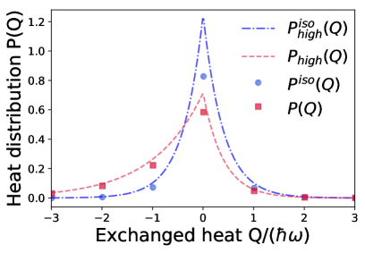
Figure 1: Asymptotic quantum quantum heat distribution $P(Q)$, Eq. (Heat distribution of a quantum harmonic oscillator), for a harmonic oscillator at inverse temperature $\beta_{1}$ weakly coupled to a bath at inverse temperature $\beta_{2}$ (red squares), compared with the symmetric isothermal heat distribution $P^{\text{iso}}(Q)$, Eq. (11), obtained for $\beta=\beta_{1}=\beta_{2}$ (blue dots). The respective blue dotted-dashed and red dashed lines represent the corresponding classical heat distribution given by Eq. (12). Parameters are $\beta_{1}=1$, $\beta_{2}=2.5$ and $\beta=2.5$.

The heat distribution (1) follows with $p_{n}(0)=1$ as,

$$P(Q,\tau)=\frac{1}{Z}\sum_{n,m}\delta[Q-(E_{m}-E_{n})]X_{m,n}(\tau)e^{-\beta_{1}\hbar\omega n}.$$ (5)

In order to analyze Eq. (5), we introduce the characteristic function $G(\mu,\tau)=\int dQ\exp({i\mu Q)P(Q,\tau)}$ and obtain,

$$G(\mu,\tau)=\frac{1}{Z}\sum_{n,m}X_{m,n}(\tau)e^{-\beta_{1}\hbar\omega n}e^{i\mu\hbar\omega(m-n)}.$$ (6)

The three sums appearing in Eq. (6) can be performed explicitly, see details below, leading to,

$$G(\mu,\tau)=\frac{\left(e^{\beta_{1}\hbar\omega}-1\right)e^{i\hbar\mu\omega}}{e^{i\hbar\mu\omega}[(u+1)e^{\beta_{1}\hbar\omega}-ue^{\hbar\omega(\beta_{1}+i\mu)}+v]-v-1}$$ (7)

The above expressions are exact and fully characterize the quantum heat fluctuations of a damped harmonic oscillator coupled to a reservoir at a different temperature. The characteristic function (7) satisfies the symmetry relation $G(i\Delta\beta-\mu,\tau)=G(\mu,\tau)$. We thus recover the fluctuation theorem for heat exchange, $P(Q,\tau)/P(-Q,\tau)=\exp(-\Delta\beta Q)$, derived by Jarzynski and Wójcik jar04 . In order to gain additional physical insight about the quantum heat statistics, we will now study different limits where closed form formulas can be derived.

We start by examining the long-time behavior of the heat statistics. In the limit $\tau\rightarrow\infty$, Eq. (7) reduces to,

$$G(\mu) = \frac{1}{Z}\sum_{n,m}e^{\beta_{1}\hbar\omega}e^{-i\mu\hbar\omega n}\left(\frac{\bar{n}}{1+\bar{n}}\right)^{m}\frac{1}{1+\bar{n}}$$

$$= \frac{1-e^{-\hbar\omega\beta_{1}}-e^{-\hbar\omega\beta_{2}}+e^{-\hbar\omega(\beta_{1}+\beta_{2})}}{1-e^{-\hbar\omega(\beta_{2}-i\mu)}-e^{-\hbar\omega(\beta_{1}+i\mu)}+e^{-\hbar\omega(\beta_{1}+\beta_{2})}}.$$

Taking the inverse Fourier transform, we arrive at the asymptotic quantum heat distribution,

$$P(Q) = \frac{1-e^{-\hbar\omega\beta_{1}}-e^{-\hbar\omega\beta_{2}}+e^{-\hbar\omega(\beta_{1}+\beta_{2})}}{1-e^{-\hbar\omega(\beta_{1}+\beta_{2})}}$$

$$\times \sum_{n}\delta(Q-n\hbar\omega)+\delta(Q+n\hbar\omega)\begin{cases}e^{-\beta_{2}Q},&Q\geq 0\\ e^{\beta_{1}Q},&Q<0\end{cases}$$

In the isothermal case, $\beta=\beta_{1}=\beta_{2}$, the characteristic function (Heat distribution of a quantum harmonic oscillator) further simplifies to,

$$G^{\text{iso}}(\mu)=\frac{\cosh(\hbar\omega\beta)-1}{\cosh(\hbar\omega\beta)-\cos(\hbar\omega\mu)}.$$ (10)

The corresponding probability distribution then reads,

$$P^{\text{iso}}(Q) = \frac{\cosh(\hbar\omega\beta)-1}{\sinh(\hbar\omega\beta)}e^{-\beta|Q|}$$ (11)

$$\times \sum_{n}\delta(Q-n\hbar\omega)+\delta(Q+n\hbar\omega).$$

Equations (Heat distribution of a quantum harmonic oscillator) and (11) are shown in Fig. 1. We observe that the two heat distributions are discrete with spacing $\hbar\omega$, as expected for a quantized harmonic oscillator. We further note that they both decay exponentially for positive and negative arguments. In addition, the heat probability density is in general asymmetric, implying a non-zero mean heat current between oscillator and bath, except in the isothermal case since no average energy flows between two objects at the same temperature.

In the high-temperature limit, $\hbar\omega\beta_{1,2}\ll 1$, the discrete heat distribution (Heat distribution of a quantum harmonic oscillator) becomes continuous and we recover the known classical expression mar15 by Taylor expanding the exponential functions to lowest order,

$$P_{\text{high}}(Q)=\frac{\beta_{1}\beta_{2}}{\beta_{1}+\beta_{2}}\begin{cases}e^{-\beta_{2}Q},&Q\geq 0,\\ e^{\beta_{1}Q},&Q<0.\end{cases}$$ (12)

As seen in Fig. 1, the envelops of the classical and quantum heat distributions are similar in shape, in contrast to the work distribution def08 . The notable difference is that the quantum density is always narrower than the corresponding classical density, owing to the bosonic nature of the harmonic oscillator. In the opposite low-temperature regime, $\hbar\omega\beta_{1,2}\gg 1$, only the first three delta peaks at $Q=0,\pm\hbar\omega$ contribute significantly to the heat distribution. As a result, we obtain the heat probability density,

$$P_{\text{low}}(Q) = \frac{\delta(Q)+\delta(Q-\hbar\omega)+\delta(Q+\hbar\omega)}{1+e^{-\hbar\omega\beta_{1}}+e^{-\hbar\omega\beta_{2}}}$$ (13)

$$\times \begin{cases}e^{-\beta_{2}Q},&Q\geq 0\\ e^{\beta_{1}Q},&Q<0\end{cases}$$

Expression (13) shows that quantum heat is strictly negative when the harmonic oscillator is initially in its ground state. This corresponds to the limiting situation where the quantum oscillator can only absorb energy.

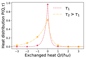
Figure 2: Evolution of the quantum heat distribution $P(Q,\tau)$ computed as the inverse Fourier transform of the characteristic function $G(\mu,\tau)$, Eq. (7), for two thermalization times $\tau_{1}=0.1$ and $\tau_{2}=2$. Parameters are $\beta_{1}=1$, $\beta_{2}=3$.

It does not seem possible to analytically determine the quantum heat distribution $P(Q,\tau)$ for arbitrary thermalization times $\tau$ (see Fig. 2). In order to study its time evolution, we next compute its first two cumulants using the formula $\left\langle Q^{n}\right\rangle(\tau)=i^{-n}d^{n}G(\mu,\tau)/d\mu^{n}{|\mu=0}$ ris89 . We obtain the average heat,

$$\langle Q\rangle(\tau)=\frac{\hbar\omega\left(ue^{\beta_{1}\hbar\omega}-v-1\right)}{e^{\beta_{1}\hbar\omega}-1},$$ (14)

and the variance,

$$\sigma^{2}_{Q}(\tau)=\left\langle Q^{2}\right\rangle(\tau)-\left\langle Q\right\rangle^{2}(\tau)=\frac{\hbar^{2}\omega^{2}\left[u(u+1)e^{2\beta_{1}\hbar\omega}+(1-u(2v+3)+v)e^{\beta_{1}\hbar\omega}+v^{2}+v\right]}{\left(e^{\beta_{1}\hbar\omega}-1\right)^{2}}.$$ (15)

in terms of the time-dependent parameters $u$ and $v$ given in Eq. (4). The variance increases as a function of time (see Fig. 3), indicating that the heat distribution widens. This can be physically understood by noting that no heat is exchanged between oscillator and reservoir when they are initially brought into thermal contact. The initially heat distribution is accordingly a Dirac delta with vanishing variance. As time increases, both mean and variance approach their stationary values exponentially, as expected for a linear system. The asymptotic long-time limits of Eqs. (14) and (15) are respectively,

$$\langle Q\rangle=\frac{1}{2}\hbar\omega\left[\coth\left(\frac{\beta_{2}\hbar\omega}{2}\right)-\coth\left(\frac{\beta_{1}\hbar\omega}{2}\right)\right],$$ (16)

and

$$\sigma^{2}_{Q}=\frac{\hbar^{2}\omega^{2}\left[-4e^{\hbar\omega(\beta_{1}+\beta_{2})}+e^{\hbar\omega(2\beta_{1}+\beta_{2})}+e^{\hbar\omega(\beta_{1}+2\beta_{2})}+e^{\beta_{1}\hbar\omega}+e^{\beta_{2}\hbar\omega}\right]}{\left(e^{\beta_{1}\hbar\omega}-1\right)^{2}\left(e^{\beta_{2}\hbar\omega}-1\right)^{2}}.$$ (17)

Equation (16) is simply the difference between the mean energies at temperatures $T_{2}$ and $T_{1}$ and can be rewritten in terms of the thermal occupation probabilities as $\langle Q\rangle=\hbar\omega(\bar{n}_{2}-\bar{n}_{1})$. We additionally notice that the heat fluctuations, as characterized by the variance, are left invariant when the temperatures of the harmonic oscillator and of the heat reservoir are switched. This is not the case for the average value of the heat which changes its sign, indicating a reversal of the energy current.

Figure 3: The variance $\sigma^{2}_{Q}(\tau)$, Eq. (15), (red solid) approaches its steady state value $\sigma^{2}_{Q}$, Eq. (17), (orange dashed) exponentially in time. The inset shows the exponential relaxation of the mean $\langle Q\rangle(\tau)$, Eq. (14), (red solid) to its asymptotic value $\langle Q\rangle$, Eq. (16), (orange dashed). Same parameters as in Fig. 2.

Conclusions. We have analytically computed the characteristic function of the quantum heat statistics of a harmonic oscillator weakly coupled to a heat reservoir at a different temperature. We have first shown that it satisfies the fluctuation theorem of Jarzynski and Wójcik jar04 . We have additionally obtained closed form expressions for the quantum heat distribution in the asymptotic long-time limit, both in the low and high temperature regimes. The classical and quantum heat probability densities have the same exponential, and generally asymmetric, dependence on $Q$. The quantum distribution is discrete with spacing corresponding to the level interval of the harmonic oscillator. It is moreover narrower than the classical distribution. We have finally investigated the time evolution of the quantum heat distribution by evaluating its first cumulants. We have shown that the stationary limit is reached exponentially in time.

Appendix. Let us sketch the derivation of the characteristic function (7). We first write Eq. (6) in terms of the ordinary hypergeometric function $F[a,b,c;z]$ whi27 ,

$$G(\mu,\tau) = \frac{1}{Z}\sum_{m,n}\frac{u^{m}}{(1+u)^{m+1}}\left(\frac{1+v}{1+u}\right)^{n}e^{-\hbar\omega\beta_{1}}$$ (18)

$$\times e^{i\hbar\omega\mu(m-n)}F\left[-n,-m,1;y\right],$$

where we have defined the variable $y=(u-v)/u(1+v)$. We next use the identity,

$$F\left[-n,-m,1;y\right]=\left(1-y\right)^{1+m+n}F\left[1+n,1+m,1;y\right]$$ (19)

together with the explicit series representation of the ordinary hypergeometric function,

$$F\left[1+n,1+m,1;y\right]=\sum_{k=0}^{\infty}y^{k}\binom{n+k}{k}\binom{m+k}{k}.$$ (20)

We then obtain the characteristic function,

$$G(\mu,\tau) = \frac{1-y}{Z(1+u)}\sum_{k}y^{k}$$ (21)

$$\times \sum_{n}\left(\frac{(1+v)(1-y)}{1+u}e^{-\hbar\omega(\beta_{1}+i\mu)}\right)^{n}\binom{n+k}{k}$$

$$\times \sum_{m}\left(\frac{u(1-y)}{1+u}e^{i\mu\hbar\omega}\right)^{m}\binom{m+k}{k}.$$

The two sums over $m$ and $n$ are of the form,

$$\sum_{j=0}^{\infty}a^{j}\binom{j+k}{k}=\left(1-a\right)^{-k-1},\quad|a|\leq 1.$$ (22)

As a consequence, we find,

$$G(\mu,\tau)=\frac{1-y}{Z(1+u)}\sum_{k}y^{k}(1-B)^{-k-1}(1-C)^{-k-1},$$ (23)

where we used introduced the two parameters,

$$B=\frac{u(1-y)}{1+u}e^{i\hbar\omega\mu},\quad C=\frac{(1+v)(1-y)}{1+u}e^{-\hbar\omega(\beta_{1}+i\mu)}$$ (24)

The final sum is a geometric series. We thus arrive at,

$$G(\mu,\tau)=\frac{1-y}{Z(1+u)}\cdot\frac{1}{(1-C)(1-B)-y}.$$ (25)

The characteristic function (7) follows by inserting the values of $B$ and $C$ given in Eq. (28) into Eq. (29).

We thank Hans C. Fogedby for attracting our attention to the quantum heat distribution. TD acknowledges financial support from the Volkswagen Foundation under project ”Quantum coins and nano sensors”.

References

(1) H. B. Callen, Thermodynamics and an Introduction to Thermostatistics, (Wiley, New York, 1985).
(2) U. Seifert, Rep. Prog. Phys. 75, 126001 (2012).
(3) K. Sekimoto, Prog. Theor. Phys. Supp. 130, 17 (1998).
(4)M. Esposito, U. Harbola and S. Mukamel, Rev. Mod. Phys. 81, 1665 (2009).
(5) M. Campisi, P. Hänggi, and P. Talkner, Rev. Mod. Phys., 83 771 (2011).
(7) S. Ciliberto, R. Gomez-Solano, and A. Petrosyan, Annu. Rev. Condens. Matter Phys. 4, 235 (2013).
(8) S. Ciliberto, Phys. Rev. X 7, 021051, (2017).
(9) R. van Zon and E. G. D. Cohen, Phys. Rev. E 69, 056121 (2004).
(10) R. van Zon, S. Ciliberto, and E. G. D. Cohen, Phys. Rev. Lett. 92, 130601 (2004).
(11) H. C. Fogedby and A. Imparato, J. Phys. A 42 475004 (2009).
(12) D. Chatterjee and B. J. Cherayil, Phys. Rev. E 82 051104 (2010).
(13) J. R. Gomez-Solano, A. Petrosyan, and S. Ciliberto, Phys. Rev. Lett. 106, 200602 (2011).
(14) S. Ciliberto, A. Imparato, A. Naert, and M. Tanase, Phys. Rev. Lett. 110, 180601 (2013).
(15) A. Imparato, L. Peliti, G. Pesce, G. Rusciano, and A. Sasso, Phys. Rev. E 76, 050101 (2007).
(16) I. A. Martinez, E. Roldan, L. Dinis, D. Petrov, and R. A. Rica, Phys. Rev. Lett. 114, 120601 (2015).
(17) S. Deffner and E. Lutz, Phys. Rev. E 77, 021128 (2008).
(18) P. Talkner, P. S. Burada, and P. Hänggi, Phys. Rev. E 78, 011115 (2009).
(19) S. Deffner, O. Abah, and E. Lutz, Chem. Phys. 375, 200 (2010).
(20) S. An, J. Zhang, M. Um, D. Lv, Y. Lu, J. Zhang, Z. Yin, H. T. Quan, and K. Kim, Nature Phys. 11, 193 (2015).
(21) P. Solinas, D. V. Averin, and J. P. Pekola, Phys. Rev. B 87, 060508(R) (2013).
(22) F. W. J. Hekking and J. P. Pekola, Phys. Rev. Lett. 111, 093602 (2013).
(23) T. B. Batalhao, A. M. Souza, L. Mazzola,
R. Auccaise, R. S. Sarthour, I. S. Oliveira, J. Goold, G. De Chiara, M. Paternostro, and R. M. Serra, Phys. Rev. Lett. 113, 140601 (2014).
(24) F. Cerisola, Y. Margalit, S. Machluf, A. J. Roncaglia, J. P. Paz, and R. Folman, Nature Commun. 8,
1241 (2017).
(25) S. Gasparinetti, P. Solinas, A. Braggio, and M. Sassetti, New J. Phys. 16, 115001 (2014).
(26) V. V. Ponomarenko, Phys. Rev. B 92, 045428 (2015).
(27) J. P. S. Peterson, T. B. Batalhao, M. Herrera, A. M. Souza, R. S. Sarthour, I. S. Oliveira, and R. M. Serra, arXiv:1803.06021.
(28) U. Weiss, Quantum Dissipative Systems, (World Scientific, Singapore, 2008).
(29) D. F. Walls and G. J Milburn, Quantum Optics, (Springer, Berlin, 2008).
(30) C. Jarzynski and D. K. Wójcik, Phys. Rev. Lett. 92, 230602 (2004).
(31) H. F. Arnoldus, J. Opt. Soc. Am. B 13, 1099 (1996).
(32) H. Risken, The Fokker-Planck Equation, (Springer, Berlin, 1989).
(33) E. T. Whittaker ans G. N. Watson, A Course of Modern Analysis, (Cambridge University Press, Cambridge, 1927).