Dual optimization for convex constrained objectives
without the gradient-Lipschitz assumption

Abstract

The minimization of convex objectives coming from linear supervised learning problems, such as penalized generalized linear models, can be formulated as finite sums of convex functions. For such problems, a large set of stochastic first-order solvers based on the idea of variance reduction are available and combine both computational efficiency and sound theoretical guarantees (linear convergence rates) [19], [35], [36], [13]. Such rates are obtained under both gradient-Lipschitz and strong convexity assumptions. Motivated by learning problems that do not meet the gradient-Lipschitz assumption, such as linear Poisson regression, we work under another smoothness assumption, and obtain a linear convergence rate for a shifted version of Stochastic Dual Coordinate Ascent (SDCA) [36] that improves the current state-of-the-art. Our motivation for considering a solver working on the Fenchel-dual problem comes from the fact that such objectives include many linear constraints, that are easier to deal with in the dual. Our approach and theoretical findings are validated on several datasets, for Poisson regression and another objective coming from the negative log-likelihood of the Hawkes process, which is a family of models which proves extremely useful for the modeling of information propagation in social networks and causality inference [12], [14].

1 Introduction

In the recent years, much effort has been made to minimize strongly convex finite sums with first order information. Recent developments, combining both numerical efficiency and sound theoretical guarantees, such as linear convergence rates, include SVRG [19], SAG [35], SDCA [36] or SAGA [13] to solve the following problem:

$$\min_{w\in\mathbb{R}^{d}}\;\;\frac{1}{n}\sum_{i=1}^{n}\varphi_{i}(w)+\lambda g(w),$$ (1)

where the functions $\varphi_{i}$ correspond to a loss computed at a sample $i$ of the dataset, and $g$ is a (eventually non-smooth) penalization. However, theoretical guarantees about these algorithms, such as linear rates guaranteeing a numerical complexity $O(\log(1/\varepsilon))$ to obtain a solution $\varepsilon$-distant to the minimum, require both strong convexity of $\frac{1}{n}\sum_{i=1}^{n}\varphi_{i}+\lambda g$ and a gradient-Lipschitz property on each $\varphi_{i}$, namely $\|\varphi_{i}^{\prime}(x)-\varphi_{i}^{\prime}(y)\|\leq L_{i}\|x-y\|$ for any $x,y\in\mathbb{R}^{d}$, where $\|\cdot\|$ stands for the Euclidean norm on $\mathbb{R}^{d}$ and $L_{i}>0$ is the Lipschitz constant. However, some problems, such as the linear Poisson regression, which is of practical importance in statistical image reconstruction among others (see [6] for more than a hundred references) do not meet such a smoothness assumption. Indeed, we have in this example $\varphi_{i}(w)=w^{\top}x_{i}-y_{i}\log(w^{\top}x_{i})$ for $i=1,\ldots,n$ where $x_{i}\in\mathbb{R}^{d}$ are the features vectors and $y_{i}\in\mathbb{N}$ are the labels, and where the model-weights must satisfy the linear constraints $w^{\top}x_{i}>0$ for all $i=1,\ldots,n$.

Motivated by machine learning problems described in Section 4 below, that do not satisfy the gradient-Lipschitz assumption, we consider a more specific task relying on a new smoothness assumption. Given convex functions $f_{i}:\mathcal{D}_{f}\rightarrow\mathbb{R}$ with $\mathcal{D}_{f}=(0,+\infty)$ such that $\lim_{t\rightarrow 0}f_{i}(t)=+\infty$, a vector $\psi\in\mathbb{R}^{d}$, features vectors $x_{1},\ldots,x_{n}\in\mathbb{R}^{d}$ corresponding to the rows of a matrix $X$ we consider the objective

$$\min_{w\in\Pi(X)}P(w)\quad\text{where}\quad P(w)=\psi^{\top}w+\frac{1}{n}\sum_{i=1}^{n}f_{i}(w^{\top}x_{i})+\lambda g(w),$$ (2)

where $\lambda>0$, $g:\mathbb{R}^{d}\rightarrow\mathbb{R}$ is a $1$-strongly convex function and $\Pi(X)$ is the open polytope

$$\Pi(X)=\{w\in\mathbb{R}^{d}\;:\;\forall i\in\{1,\dots,n\},\;w^{\top}x_{i}>0\},$$ (3)

that we assume to be non-empty. Note that the linear term $\psi^{\top}w$ can be included in the regularization $g$ but the problem stands clearer if it is kept out.

Definition 1.

We say that a function $f:\mathcal{D}_{f}\subset\mathbb{R}\rightarrow\mathbb{R}$ is $L$-$\log$ smooth, where $L>0$, if it is a differentiable and strictly monotone convex function that satisfies

$$|f^{\prime}(x)-f^{\prime}(y)|\leq\frac{1}{L}f^{\prime}(x)f^{\prime}(y)|x-y|$$

for all $x,y\in\mathcal{D}_{f}$.

We detail this property and its specificities in Section 2. All along the chapter, we assume that the functions $f_{i}$ are $L_{i}$-$\log$ smooth. Note also that the Poisson regression objective fits in this setting, where $f_{i}(x)=-y_{i}\log x$ is $y_{i}$-$\log$ smooth and $\psi=\frac{1}{n}\sum_{i=1}^{n}x_{i}$. See Section 4.1 below for more details.

Related works.

Standard first-order batch solvers (non stochastic) for composite convex objectives are ISTA and its accelerated version FISTA [5] and first-order stochastic solvers are mostly built on the idea of Stochastic Gradient Descent (SGD) [34]. Recently, stochastic solvers based on a combination of SGD and the Monte-Carlo technique of variance reduction [35], [36], [19], [13] turn out to be both very efficient numerically (each update has a complexity comparable to vanilla SGD) and very sound theoretically, because of strong linear convergence guarantees, that match or even improve the one of batch solvers. These algorithms involve gradient steps on the smooth part of the objective and theoretical guarantees justify such steps under the gradient-Lipschitz assumptions thanks to the descent lemma [7, Proposition A.24]. Without this assumption, such theoretical guarantees fall apart. Also, stochastic algorithms loose their numerical efficiency if their iterates are projected on the feasible set $\Pi(X)$ at each iteration as Equation (2) requires. STORC [18] can deal with constrained objectives without a full projection but is restricted to compact sets of constraints which is not the case of $\Pi(X)$. Then, a modified proximal gradient method from [40] provides convergence bounds relying on self-concordance [26] rather than the gradient-Lipschitz property. However, the convergence rate is guaranteed only once the iterates are close to the optimal solution and we observed in practice that this algorithm is simply not working (since it ends up using very small step-sizes) on the problems considered here. Recently, [21] has provided new descent lemmas based on relative-smoothness that hold on a wider set of functions including Poisson regression losses. This work is an extension of [4] that presented the same algorithm and detailed its application to Poisson regression losses. While this is more generic than our work, they only manage to reach sublinear convergence rates $\mathcal{O}(1/t)$ that applies only on positive solution (namely $w^{*}\in[0,\infty)^{d}$) while we reach linear rates for any solution $w^{*}\in\mathbb{R}^{d}$.

Our contribution.

The first difficulty with the objective (2) is to remain in the open polytope $\Pi(X)$. To deal with simpler constraints we rather perform optimization on the dual problem

$$\max_{\alpha\in-\mathcal{D}_{f^{*}}^{n}}D(\alpha)\quad\text{where}\quad D(\alpha)=\frac{1}{n}\sum_{i=1}^{n}-f^{*}_{i}(-\alpha_{i})-\lambda g^{*}\Bigg{(}\frac{1}{\lambda n}\sum_{i=1}^{n}\alpha_{i}x_{i}-\frac{1}{\lambda}\psi\Bigg{)},$$ (4)

where for a function $h$, the Fenchel conjugate $h^{*}$ is given by $h^{*}(v)=\sup_{u}uv-h(u)$, and $-\mathcal{D}_{f^{*}}$ is the domain of the function $x\mapsto\sum_{i=1}^{n}f_{i}^{*}(-x)$. This strategy is the one used by Stochastic Dual Coordinate Ascent (SDCA) [36]. The dual problem solutions are box-constrained to $-\mathcal{D}_{f^{*}}^{n}$ which is much easier to maintain than the open polytope $\Pi(X)$. Note that as all $f_{i}$ are strictly decreasing (because they are strictly monotone on $(0,+\infty)$ with $\lim_{t\rightarrow 0}f_{i}(t)=+\infty$), their dual are defined on $\mathcal{D}_{f^{*}}\subset(-\infty,0)$. By design, this approach keeps the dual constraints maintained all along the iterations and the following proposition, proved in Section 7.1, ensures that the primal iterate converges to a point of $\Pi(X)$.

Proposition 1.

Assume that the polytope $\Pi(X)$ is non-empty, the functions $f_{i}$ are convex, differentiable, with $\lim_{t\rightarrow 0}f_{i}(t)=+\infty$ for $i=1,\dots,n$ and that $g$ is strongly convex. Then, strong duality holds, namely $P(w^{*})=D(\alpha^{*})$ and the Karush-Kuhn-Tucker conditions relate the two optima as

$$\forall i\in\{1,\dots,n\},\;\alpha_{i}^{*}=-{f_{i}^{*}}^{\prime}({w^{*}}^{\top}x_{i})\quad\text{and}\quad w^{*}=\nabla g^{*}\bigg{(}\frac{1}{\lambda n}\sum_{i=1}^{n}\alpha_{i}x_{i}-\frac{1}{\lambda}\psi\bigg{)},$$

where $w^{*}\in\Pi(X)$ is the minimizer of $P$ and $\alpha^{*}\in-\mathcal{D}_{f^{*}}^{n}$ the maximizer of $D$.

In this chapter, we introduce the $\log$ smoothness property and its characteristics and then we derive linear convergence rates for SDCA without the gradient-Lipschitz assumption, by replacing it with $\log$ smoothness, see Definition 1. Our results provide a state-of-the-art optimization technique for the considered problem (2), with sound theoretical guarantees (see Section 3) and very strong empirical properties as illustrated on experiments conducted with several datasets for Poisson regression and Hawkes processes likelihood (see Section 5). We study also SDCA with importance sampling [42] under $\log$ smoothness and prove that it improves both theoretical guarantees and convergence rates observed in practical situations, see Sections 3.2 and 5. We provide also a heuristic initialization technique in Section 5.3 and a "mini-batch" [32] version of the algorithm in Section 5.4 that allows to end up with a particularly efficient solver for the considered problems. We motivate even further the problem considered in this chapter in Figure 1, where we consider a toy Poisson regression problem (with 2 features and 3 data points), for which L-BFGS-B typically fails while SDCA works. This illustrates the difficulty of the problem even on such an easy example.

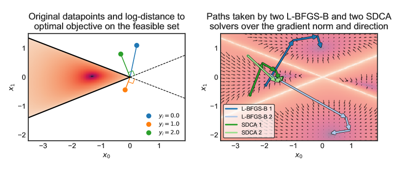
Figure 1: Iterates of SDCA and L-BFGS-B on a Poisson regression toy example with three samples and two features. Left. Dataset and value of the objective. Right: Iterates of L-BFGS-B and SDCA with two different starting points. The background represents the gradient norm and the arrows the gradient direction. SDCA is very stable and converges quickly towards the optimum, while L-BFGS-B easily converges out of the feasible space.

Outline.

We first introduce the $\log$ smoothness property in Section 2, relate it to self-concordance in Proposition 2 and translate it in the Fenchel conjugate space in Proposition 3. Then, we present the shifted SDCA algorithm in Section 3 and state its convergence guarantees in Theorem 4 under the $\log$ smoothness assumption. We also provide theoretical guarantees for variants of the algorithm, one using proximal operators [37] and the second using importance sampling [42] which leads to better convergence guarantees in Theorem 5. In Section 4 we focus on two specific problems, namely Poisson regression and Hawkes processes, and explain how they fit into the considered setting. Section 5 contains experiments that illustrate the benefits of our approach compared to baselines. This Section also proposes a very efficient heuristic initialization and numerical details allowing to optimize over several indices at each iteration, which is a trick to accelerate even further the algorithm.

2 A tighter smoothness assumption

To have a better overview of what $\log$ smoothness is, we formulate the following proposition giving an equivalent property for $\log$ smooth functions that are twice differentiable.

Proposition 2.

Let $f:\mathcal{D}_{f}\subset\mathbb{R}\rightarrow\mathbb{R}$ be a convex strictly monotone and twice differentiable function. Then,

$$f\text{ is $L$-$\log$ smooth}\quad\Leftrightarrow\quad\forall x\in\mathcal{D}_{f},\;f^{\prime\prime}(x)\leq\tfrac{1}{L}f^{\prime}(x)^{2}.$$

This proposition is proved in Section 7.4 and we easily derive from it that ${x\mapsto-L\log x}$ on $(0,+\infty)$, $x\mapsto Lx$ on $\mathbb{R}$ and $x\mapsto L\exp(x)$ on $[0,+\infty)$ are $L$-$\log$ smooth. This proposition is linked to the self-concordance property introduced by Nesterov [26] widely used to study losses involving logarithms. For the sake of clarity, the results will be presented for functions whose domain $\mathcal{D}_{f}$ is a subset of $\mathbb{R}$ as this leads to lighter notations.

Definition 2.

A convex function $f:\mathcal{D}_{f}\subset\mathbb{R}\rightarrow\mathbb{R}$ is standard self-concordant if

$$\forall x\in\mathcal{D}_{f},\;|f^{\prime\prime\prime}(x)|\leq 2f^{\prime\prime}(x)^{3/2}.$$

This property has been generalized [1, 38] but always consists in controlling the third order derivative by the second order derivative, initially to bound the second order Taylor approximation used in the Newton descent algorithm [26]. While right hand sides of both properties ($f^{\prime}(x)^{2}$ and $2f^{\prime\prime}(x)^{3/2}$) might look arbitrarily chosen, in fact they reflect the motivating use case of the logarithmic barriers where $f:t\mapsto-\log(t)$ and for which the bound is reached. Hence, $\log$ smoothness is the counterpart of self-concordance but to control the second order derivative with the first order derivative. As it is similarly built, $\log$ smoothness shares the affine invariant property with self-concordance. It means that if $f_{1}$ is $L$ $\log$-smooth then $f_{2}:x\mapsto ax+b$ with $a,b\in\mathbb{R}$ is also $L$-$\log$ smooth with the same constant $L$. An extension to the multivariate case where $\mathcal{D}_{f}\subset\mathbb{R}^{d}$ is likely feasible but is useless for our algorithm and hence beyond the scope of this paper. From the $\log$ smoothness property of a function $f$, we derive several characteristics for its Fenchel conjugate $f^{*}$ starting with the following proposition.

Proposition 3.

Let $f:\mathcal{D}_{f}\subset\mathbb{R}\rightarrow\mathbb{R}$ be a strictly monotone convex function and $f^{*}$ be its twice differentiable Fenchel conjugate. Then,

$$f\text{ is $L$-$\log$ smooth}\quad\Leftrightarrow\quad\exists L>0;\;\forall x\in\mathcal{D}_{f^{*}},\;{f^{*}}^{\prime\prime}(x)\geq Lx^{-2}.$$

This proposition is proved in Section 7.5 and is the first step towards a series of convex inequalities for the Fenchel conjugate of $\log$ smooth functions. These inequalities, detailed in Section 7.6, bounds the Bregman divergence of such functions and are compared to what can be obtained with self-concordance or strong convexity (on a restricted set) in the canonical case where $f:t\mapsto-\log(t)$. It appears with $\log$ smoothness we obtain tighter bounds than what is achievable with other assumptions and that all these bounds are reached (and hence cannot be improved) in the canonical case (see Table 3).

3 The Shifted SDCA algorithm

The dual objective (4) cannot be written as a composite sum of convex functions as in the general objective (1), which is required for stochastic algorithms such as SRVG [19] or SAGA [13]. It is better to use a coordinate-wise approach to optimize this problem, which leads to SDCA [37], in which the starting point has been shifted by $\frac{1}{\lambda}\psi$. This shift is induced by the relation linking primal and dual variables at the optimum: the second Karush-Kuhn-Tucker condition from Proposition 1,

$$w^{*}=\nabla g^{*}\bigg{(}\frac{1}{\lambda n}\sum_{i=1}^{n}\alpha_{i}^{*}x_{i}-\frac{1}{\lambda}\psi\bigg{)}.$$ (5)

We first present the general algorithm (Algorithm 1), then its proximal alternative (Algorithm 2) and finally how importance sampling leads to better theoretical results. We assume that we know bounds $(\beta_{i})_{1\leq i\leq n}$ such that $\beta_{i}/\alpha_{i}^{*}\geq 1$ for any $i=1,\ldots,n$, such bounds can be explicitly computed from the data in the particular cases considered in this chapter, see Section 4 for more details.

Algorithm 1 Shifted SDCA

1: Bounds $\beta_{i}\in-\mathcal{D}_{f^{*}}$ such that $\forall i\in\{1,\dots,n\},~{}\beta_{i}/\alpha_{i}^{*}\geq 1$, $\alpha^{(0)}\in-\mathcal{D}_{f^{*}}^{n}$ dual starting point such that $\forall i\in\{1,\dots,n\},~{}\beta_{i}/\alpha_{i}\geq 1$

2:$v^{(0)}=\frac{1}{\lambda n}\sum_{i=1}^{n}\alpha_{i}^{(0)}x_{i}-\frac{1}{\lambda}\psi$

3:for $t=1,2\dots T$ do

4:     Sample $i$ uniformly at random in $\{1,\ldots,n\}$

5:     Find $\alpha_{i}$ that maximizes $-\frac{1}{n}f_{i}^{*}(-\alpha_{i})-\lambda g^{*}\big{(}v^{(t-1)}+(\lambda n)^{-1}(\alpha_{i}-\alpha_{i}^{(t-1)})x_{i}\big{)}$

6:     $\alpha_{i}\leftarrow\min(1,\beta_{i}/\alpha_{i})\alpha_{i}$

7:     $\Delta\alpha_{i}\leftarrow\alpha_{i}-\alpha_{i}^{(t-1)}$

8:     $\alpha^{(t)}\leftarrow\alpha^{(t-1)}+\Delta\alpha_{i}e_{i}$

9:     $v^{(t)}\leftarrow v^{(t-1)}+(\lambda n)^{-1}\Delta\alpha_{i}x_{i}$

10:     $w^{(t)}\leftarrow\nabla g^{*}(v^{(t)})$

11:end for

The next theorem provides a linear convergence rate for Algorithm 1 where we assume that each $f_{i}$ is $L_{i}$-$\log$ smooth (see Definition 1).

Theorem 4.

Suppose that we known bounds $\beta_{i}\in-\mathcal{D}_{f^{*}}$ such that $R_{i}=\frac{\beta_{i}}{\alpha_{i}^{*}}\geq 1$ for $i=1,\dots,n$ and assume that all $f_{i}$ are $L_{i}$-$\log$ smooth with differentiable Fenchel conjugates and $g$ is 1-strongly convex. Then, Algorithm 1 satisfies

$$\mathbb{E}[D(\alpha^{*})-D(\alpha^{(t)})]\leq\Big{(}1-\frac{\min_{i}\sigma_{i}}{n}\Big{)}^{t}(D(\alpha^{*})-D(\alpha^{(0)})),$$ (6)

where

$$\sigma_{i}=\bigg{(}1+\frac{\|x_{i}\|^{2}{\alpha_{i}^{*}}^{2}}{2\lambda nL_{i}}\frac{(R_{i}-1)^{2}}{\frac{1}{R_{i}}+\log R_{i}-1}\bigg{)}^{-1}.$$ (7)

The proof of Theorem 4 is given in Section 7.7. It states that in the considered setting, SDCA achieves a linear convergence rate for the dual objective. The bounds $\beta_{i}$ are provided in Section 4 below for two particular cases: Poisson regression and likelihood Hawkes processes. Equipped with these bounds, we can compare the rate obtained in Theorem 4 with already known linear rates for SDCA under the gradient-Lipschitz assumption [36]. Indeed, we can restrict the domain of all $f_{i}^{*}$ to $(-\beta_{i},0)$ on which Proposition 3 states that all $f_{i}$ are $L_{i}/({\alpha_{i}^{*}}^{2}R_{i}^{2})$-strongly convex. Now, following carefully the proof in [36] leads to the convergence rate given in Equation (6) but with

$$\sigma_{i}=\bigg{(}1+\frac{\|x_{i}\|^{2}{\alpha_{i}^{*}}^{2}}{\lambda nL_{i}}R_{i}^{2}\bigg{)}^{-1}.$$

Since $2\big{(}\frac{1}{R}+\log R-1\big{)}(R-1)^{-2}\geq R^{-2}$ for any $R\geq 1$, Theorem 4 provides a faster convergence rate. The comparative gain depends on the values of $(\|x_{i}\|^{2}{\alpha_{i}^{*}}^{2})/(\lambda nL_{i})$ and $R_{i}$ but it increases logarithmically with the value of $R_{i}$. Table 1 below compares the explicit values of these linear rates on a dataset used in our experiments for Poisson regression.

Remark 1.

Convergence rates for the primal objective are not provided since the primal iterate $w^{(t)}$ typically belongs to $\Pi(X)$ only when it is close enough to the optimum. This would make most of the values of the primal objective $P(w^{(t)})$ undefined and therefore not comparable to $P(w^{*})$.

3.1 Proximal algorithm

Algorithm 1 maximizes the dual over one coordinate at Line 5 whose solution might not be explicit and requires inner steps to obtain $\alpha_{i}^{(t)}$. But, whenever $g$ can be written as

$$g(w)=\tfrac{1}{2}\|w\|^{2}+h(w),$$ (8)

where $h$ is a convex, prox capable and possibly non-differentiable function, we use the same technique as Prox-SDCA [37] with a proximal lower bound that leads to

$$\alpha_{i}^{(t)}=\operatorname*{arg\,max}_{a_{i}\in-\mathcal{D}_{f^{*}}}-f^{*}_{i}(-\alpha_{i})-\frac{\lambda n}{2}\Big{\|}w^{(t-1)}-(\lambda n)^{-1}(\alpha_{i}-\alpha_{i}^{(t-1)})x_{i}\Big{\|}^{2},$$

with

$$w^{(t-1)}=\operatorname{prox}_{h}\bigg{(}\frac{1}{\lambda n}\sum_{i=1}^{n}\alpha_{i}^{(t-1)}x_{i}-\frac{1}{\lambda}\psi\bigg{)},$$

see Section 7.2 for details. This leads to a proximal variant described in Algorithm 2 below, which is able to handle various regularization techniques and which has the same convergence guarantees as Algorithm 1 given in Theorem 4. Also, note that assuming that $g$ can be written as (8) with a prox-capable function $h$ is rather unrestrictive, since one can always add a ridge penalization term in the objective.

Algorithm 2 Shifted Prox-SDCA

1: Bounds $\beta_{i}\in-\mathcal{D}_{f^{*}}$ such that $\forall i\in\{1,\dots,n\},~{}\beta_{i}/\alpha_{i}^{*}\geq 1$, $\alpha^{(0)}\in-\mathcal{D}_{f^{*}}^{n}$ dual starting point such that $\forall i\in\{1,\dots,n\},~{}\beta_{i}/\alpha_{i}\geq 1$

2:$v^{(0)}=\frac{1}{\lambda n}\sum_{i=1}^{n}\alpha_{i}^{(0)}x_{i}-\frac{1}{\lambda}\psi$

3:for $t=1,2\dots T$ do

4:     Sample $i$ uniformly at random in $\{1,\ldots,n\}$

5:     Find $\alpha_{i}$ that maximize $-\frac{1}{n}f_{i}^{*}(-\alpha_{i})-\frac{\lambda}{2}\Big{\|}w^{(t-1)}+(\lambda n)^{-1}(\alpha_{i}-\alpha_{i}^{(t-1)})x_{i}\Big{\|}^{2}$

6:     $\alpha_{i}\leftarrow\min(1,\beta_{i}/\alpha_{i})\alpha_{i}$

7:     $\Delta\alpha_{i}\leftarrow\alpha_{i}-\alpha_{i}^{(t-1)}$

8:     $\alpha^{(t)}\leftarrow\alpha^{(t-1)}+\Delta\alpha_{i}e_{i}$

9:     $v^{(t)}\leftarrow v^{(t-1)}+(\lambda n)^{-1}\Delta\alpha_{i}x_{i}$

10:     $w^{(t)}\leftarrow\operatorname{prox}_{h}(v^{(t)})$

11:end for

3.2 Importance sampling

Importance sampling consists in adapting the probabilities of choosing a sample $i$ (which is by default done uniformly at random, see Line 4 from Algorithm 1) using the improvement which is expected by sampling it. Consider a distribution $\rho$ on $\{1,\dots,n\}$ with probabilities $\{\rho_{1},\dots,\rho_{n}\}$ such that $\rho_{i}\geq 0$ for any $i$ and $\sum_{i=1}^{n}\rho_{i}=1$. The Shifted SDCA and Shifted Prox-SDCA with importance sampling algorithms are simply obtained by modifying the way $i$ is sampled in Line 4 of Algorithms 1 and 2: instead of sampling uniformly at random, we sample using such a distribution $\rho$. The optimal sampling probability $\rho$ is obtained in the same way as [42] and it also leads under our $\log$ smoothness assumption to a tighter convergence rate, as stated in Theorem 5 below.

Theorem 5.

Suppose that we known bounds $\beta_{i}\in-\mathcal{D}_{f^{*}}$ such that $R_{i}=\frac{\beta_{i}}{\alpha_{i}^{*}}\geq 1$ for $i=1,\ldots,n$ and assume that all $f_{i}$ are $L_{i}$-$\log$ smooth with differentiable Fenchel conjugates and $g$ is 1-strongly convex. Consider $\sigma$ defined by (7) and consider the distribution

$$\rho_{i}=\frac{\sigma_{i}^{-1}}{\sum_{j=1}^{n}\sigma_{j}^{-1}}$$

for $i\in\{1,\ldots,n\}$. Then, Algorithm 1 and 2 where Line 4 is replaced by sampling $i\sim\rho$ satisfy

$$\mathbb{E}[D(\alpha^{*})-D(\alpha^{(t)})]\leq\Big{(}1-\frac{\bar{\sigma}}{n}\Big{)}^{t}(D(\alpha^{*})-D(\alpha^{(0)}),$$

where $\bar{\sigma}=\big{(}\frac{1}{n}\sum_{i=1}^{n}\sigma_{i}^{-1}\big{)}^{-1}$.

The proof is given in Section 7.8. This convergence rate is stronger than the previous one from Theorem 4 since $(\frac{1}{n}\sum_{i=1}^{n}\sigma_{i}^{-1})^{-1}\geq\min_{i}\sigma_{i}$. Table 1 below compares the explicit values of these linear rates on a dataset used in our experiments for Poisson regression (facebook dataset). We observe that the $\log$ smooth rate with importance sampling is orders of magnitude better than the one obtained with the standard theory for SDCA which exploits only the $L_{i}/({\alpha_{i}^{*}}^{2}R_{i}^{2})$ strong convexity of the functions $f_{i}^{*}$.

strongly convex	strongly convex with	$\log$ smooth	$\log$ smooth with
	importance sampling		importance sampling
$(0.9999)^{t}$	$(0.9969)^{t}$	$(0.9984)^{t}$	$(\boldsymbol{0.9679})^{t}$

Table 1: Theoretical convergence rates obtained on the facebook dataset (see Section 5.1) in four different settings: strongly convex (which is the rate obtained when all functions $f_{i}$ are considered $L_{i}/({\alpha_{i}^{*}}^{2}R_{i}^{2})$-strongly convex) with and without importance sampling [36, 42] and the rate obtained in the setting considered in the chapter, with and without importance sampling. In this experiment, the maximum value for $R_{i}$ is 9062 and its average value is 308. As expected, the best rate is obtained by combining the $\log$-smoothness property with importance sampling.

4 Applications to Poisson regression and Hawkes processes

In this Section we describe two important models that fit into the setting of this chapter. We precisely formulate them as in Equation (2) and give the explicit value of bounds $\beta_{i}$ such as $\alpha_{i}^{*}\leq\beta_{i}$, where $\alpha^{*}$ is the solution to the dual problem (4).

4.1 Linear Poisson regression

Poisson regression is widely used to model count data, namely when, in the dataset, each observation $x_{i}\in\mathbb{R}^{d}$ is associated an integer output $y_{i}\in\mathbb{N}$ for $i=1,\dots,n$. It aims to find a vector $w\in\mathbb{R}^{d}$ such that for a given function $\phi:\mathcal{D}_{\phi}\subset\mathbb{R}\rightarrow(0,+\infty)^{+}$, $y_{i}$ is the realization of a Poisson random variable of intensity $\phi(w^{\top}x_{i})$. A convenient choice is to use $\exp$ for $\phi$ as it always guarantees that $\phi(w^{\top}x_{i})>0$. However, using the exponential function assumes that the covariates have a multiplicative effect that often cannot be justified. The tougher problem of linear Poisson regression, where $\phi(t)=t$ and $\mathcal{D}_{\phi}$ is the polytope $\Pi(X)$, appears to model additive effects. For example, this applies in image reconstruction. The original image is retrieved from photons counts $y_{i}$ distributed as a Poisson distribution with intensity $w^{\top}x_{i}$, that are received while observing the image with different detectors represented by the vectors $x_{i}\in\mathbb{R}^{d}$. This application has been extensively studied in the literature, see [16, 4, 40] and [6] for a review with a hundred references. Linear Poisson regression is also used in various fields such as survival analysis with additive effects [8] and web-marketing [9] where the intensity corresponds to an intensity of clicks on banners in web-marketing. To formalize, we consider a training dataset $(x_{1},y_{1}),\ldots,(x_{n_{0}},y_{n_{0}})$ with $x_{i}\in\mathbb{R}^{d}$ and $y_{i}\in\mathbb{N}$ and assume without loss of generality that $y_{i}>0$ for $i\in\{1,\ldots,n\}$ while $y_{i}=0$ for $i\in\{n+1,\ldots,n_{0}\}$ where $n=\#\{i:y_{i}>0\}\leq n_{0}$ (this simply means that we put first the samples corresponding to a label $y_{i}>0$). The negative log-likelihood of this model with a penalization function $g$ can be written as

$$P_{0}(w)=\frac{1}{n_{0}}\sum_{i=1}^{n_{0}}(w^{\top}x_{i}-y_{i}\log(w^{\top}x_{i}))+\lambda_{0}g(w)$$

where $\lambda_{0}>0$ corresponds to the level of penalization, with the constraint that $w^{\top}x_{i}$ for $i=1,\ldots,n$. This corresponds to Equation (2) with $f_{i}(w)=-y_{i}\log(x_{i}^{\top}w)$ for $i=1,\ldots,n$, which are $y_{i}$-$\log$ smooth functions, and with

$$\psi=\frac{1}{n}\sum_{i=1}^{n_{0}}x_{i}\quad\text{and}\quad\lambda=\frac{n_{0}}{n}\lambda_{0}.$$

Note that the zero labeled observations can be safely removed from the sum and are fully encompassed in $\psi$. The algorithms and results proposed in Section 3 can therefore be applied for this model.

4.2 Hawkes processes

Hawkes processes are used to study cross causality that might occur in one or several events series. First, they were introduced to study earthquake propagation, the network across which the aftershocks propagate can be recovered given all tremors timestamps [30]. Then, they have been used in high frequency finance to describe market reactions to different types of orders [3]. In the recent years Hawkes processes have found many new applications including crime prediction [23] or social network information propagation [22]. A Hawkes process [17] is a multivariate point-process: it models timestamps $\{t_{k}^{i}\}_{i\geq 1}$ of nodes $i=1,\ldots,I$ using a multivariate counting process with a particular auto-regressive structure in its intensity. More precisely, we say that a multivariate counting process $N_{t}=[N_{t}^{1},\ldots,N_{t}^{I}]$ where $N_{t}^{i}=\sum_{k\geq 1}\mathbf{1}_{t_{k}^{i}\leq t}$ for $t\geq 0$ is a Hawkes process if the intensity of $N^{i}$ has the following structure:

$$\lambda^{i}(t)=\mu_{i}+\sum_{j=1}^{I}\int\phi_{ij}(t-s)\mathop{}\!\mathrm{d}N^{j}(s)=\mu_{i}+\sum_{j=1}^{I}\sum_{k\;:\;t_{k}^{j}<t}\phi_{ij}(t-t_{k}^{j}).$$

The $\mu_{i}\geq 0$ are called baselines intensities, and correspond to the exogenous intensity of events from node $i$, and the functions $\phi_{ij}$ for $1\leq i,j\leq I$ are called kernels. They quantify the influence of past events from node $j$ on the intensity of events from node $i$. The main parametric model for the kernels is the so-called exponential kernel, in which we consider

$$\phi^{ij}(t)=\sum_{u=1}^{U}a_{u}^{ij}b_{u}\exp(-b_{u}t)$$ (9)

with $b_{u}>0$. In this model the matrix $A=[\sum_{u=1}^{U}a_{u}^{ij}]_{1\leq i,j\leq d}$ is understood as an adjacency matrix, since entry $A_{i,j}$ quantifies the impact of the activity of node $j$ on the activity of node $i$, while $b_{u}>0$ are memory parameters. We stack these parameters into a vector $\theta$ containing the baselines $\mu_{i}$ and the self and cross-excitation parameters $a_{u}^{ij}$. Note that in this model the memory parameters $b_{u}$ are supposed to be given. The associated goodness-of-fit is the negative log-likelihood, which is given by the general theory of point processes (see [11]) as

$$-\ell(\theta)=-\sum_{i=1}^{I}\ell_{i}(\theta),\quad\text{with}\quad-\ell_{i}(\theta)=\int_{0}^{T}\lambda_{\theta}^{i}(t)dt-\int_{0}^{T}\log(\lambda_{\theta}^{i}(t))\mathop{}\!\mathrm{d}N^{i}(t).$$

Let us define the following weights for $i,j=1,\dots I$ and $u=1,\dots,U$,

$$g^{j}_{u}(t)=\sum_{k\;:\;t_{k}^{j}<t}b_{u}e^{-b_{u}(t-t_{k}^{j})},\quad g^{ij}_{u,k}=g^{j}_{u}(t_{k}^{i})\quad\text{and}\quad G^{j}_{u}=\int_{0}^{T}g^{j}_{u}(t)dt$$ (10)

that can be computed efficiently for exponential kernels thanks to recurrence formulas (the complexity is linear with respect to the number of events of each node). Using the parametrization of the kernels from Equation (9) we can rewrite each term of the negative log-likelihood as

$$-\ell_{i}(\mu_{i},a^{i})=\sum_{i=1}^{I}\bigg{[}\mu^{i}T+\sum_{j=1}^{I}\sum_{u=1}^{U}a^{ij}_{u}G_{u}^{j}-\sum_{k=1}^{n_{i}}\log\Big{(}\mu^{i}+\sum_{j=1}^{I}\sum_{u=1}^{U}a^{ij}_{u}g^{ij}_{u,k}\Big{)}\bigg{]}.$$

To rewrite $\ell_{i}$ in a vectorial form we define $n_{i}$ as the number of events of node $i$ and the following vectors for $i=1,\dots,I$:

$$w^{i}=\begin{bmatrix}\mu^{i}&a^{i,1}_{1}&\cdots&a^{i,1}_{U}&\cdots&a^{i,I}_{1}&\cdots&a^{i,I}_{U}\end{bmatrix}^{\top},$$

that are the model weights involved in $\ell_{i}$, and

$$\psi^{i}=\frac{1}{n_{i}}\begin{bmatrix}T&G^{1}_{1}&\cdots G^{1}_{U}&\cdots&G^{I}_{1}&\cdots&G^{I}_{U}\\ \end{bmatrix}^{\top},$$

which correspond to the vector involved in the linear part of the primal objective (2) and finally

$$x^{i}_{k}=\begin{bmatrix}1&g^{i,1}_{1,k}&\cdots&g^{i,1}_{U,k}&\cdots&g^{i,I}_{1,k}&\cdots&g^{i,I}_{U,k}\\ \end{bmatrix}^{\top},$$

for $k=1,\dots,n_{i}$ which contains all the timestamps data computed in the weights computed in Equation (10). With these notations the negative log-likelihood for node $i$ can be written as

$$-\ell(w)=-\sum_{i=1}^{I}\ell_{i}(w^{i})\quad\text{with}\quad-\tfrac{1}{n_{i}}\ell_{i}(w^{i})=(w^{i})^{\top}\psi^{i}-\frac{1}{n_{i}}\sum_{k=1}^{n_{i}}\log((w^{i})^{\top}x_{k}^{i}).$$

First, it shows that the negative log-likelihood can be separated into $I$ independent sub-problems with goodness-of-fit $-\ell_{i}(w^{i})$ that corresponds to the intensity of node $i$ with the weights $x_{i,k}$ carrying data from the events of the other nodes $j$. Each subproblem is a particular case of the primal objective (2), where all the labels $y_{i}$ are equal to $1$. As a consequence, we can use the algorithms and results from Section 3 to train penalized multivariate Hawkes processes very efficiently.

4.3 Closed form solution and bounds on dual variables

In this Section with provide the explicit solution to Line 5 of Algorithm 2 when the objective corresponds to the linear Poisson regression or the Hawkes process goodness-of-fit. In Proposition 6 below we provide the closed-form solution of the local maximization step corresponding to Line 5 of Algorithm 2.

Proposition 6.

For Poisson regression and Hawkes processes, Line 5 of Algorithm 2 has a closed form solution, namely

$$\alpha^{t}_{i}=\frac{1}{2}\Bigg{(}\sqrt{\Big{(}\alpha_{i}^{(t-1)}-\frac{\lambda n}{\|x_{i}\|^{2}}x_{i}^{\top}w^{(t-1)}\Big{)}^{2}+4\lambda n\frac{y_{i}}{\|x_{i}\|^{2}}}+\alpha_{i}^{(t-1)}-\frac{\lambda n}{\|x_{i}\|^{2}}x_{i}^{\top}w^{(t-1)}\Bigg{)}.$$

This closed-form expression allows to derive a numerically very efficient training algorithm, as illustrated in Section 5 below. For these two use cases, the dual loss is given by $f_{i}^{*}(-\alpha_{i})=-y_{i}-y_{i}\log(\frac{\alpha_{i}}{y_{i}})$ for any $\alpha_{i}>0$ (with $y_{i}=1$ for the Hawkes processes). For this specific dual loss, we can provide also upper bounds $\beta_{i}$ for all optimal dual variables $\alpha_{i}^{*}$, as stated in the next Proposition.

Proposition 7.

For Poisson regression and Hawkes processes, if $g(w)=\tfrac{1}{2}\|w\|^{2}$ and if ${x_{i}}^{\top}x_{j}\geq 0$ for all $1\leq i,j\leq n$, we have the following upper bounds on the dual variables at the optimum:

$$\alpha_{i}^{*}\leq\beta_{i}\quad\text{where}\quad\beta_{i}=\frac{1}{2\|x_{i}\|^{2}}\bigg{(}n\psi^{\top}x_{i}+\sqrt{(n\psi^{\top}x_{i})^{2}+4\lambda ny_{i}\|x_{i}\|^{2}}\bigg{)}$$

for any $i=1,\ldots,n$.

The proofs of Propositions 6 and 7 are provided in Section 7.9. Note that the inner product assumption ${x_{i}}^{\top}x_{j}\geq 0$ from Proposition 7 is mild: it is always met for the Hawkes process with kernels given by (9) and it it met for Poisson regression whenever one applies for instance a min-max scaling on the features matrix.

Remark 2.

The closed form solution from Proposition 6 is always lower than the generic bound $\beta_{i}$, as explained in Section 7.11. Hence, we actually do not need to manually bound $\alpha_{i}^{(t)}$ at line 6 of Algorithm 1 in this particular case.

5 Experiments

To evaluate efficiently Shifted SDCA we have compared it with other optimization algorithms that can handle the primal problem (2) nicely, without the gradient-Lipschitz assumptions. We have discarded the modified proximal gradient method from [40] since most of the time it was diverging while computing the initial step with the Barzilai-Borwein method on the considered examples. We consider the following algorithms.

NoLips.

This is a first order batch algorithm that relies on relative-smoothness [21] instead of the gradient Lipschitz assumption. Its application to linear Poisson regression has been detailed in [4] and its analysis provides convergence guarantees with a sublinear convergence rate in $\mathcal{O}(1/n)$. However, this method is by design limited to solutions with positive entries (namely $w^{*}\in[0,\infty)^{d}$) and provides guarantees only in this case. Its theoretical step-size decreases linearly with $1/n$ and is too small in practice. Hence, we have tuned the step-size to get the best objective after 300 iterations.

SVRG.

This is a stochastic gradient descent algorithm with variance reduction introduced in [19, 41]. We used a variant introduced in [39], which uses Barzilai-Borwein in order to adapt the step-size, since gradient-Lipschitz constants are unavailable in the considered setting. We consider this version of variance reduction, since alternatives such as SAGA[13] and SAG [35] do not propose variants with Barzilai-Borwein type of step-size selection.

L-BFGS-B.

L-BFGS-B is a limited-memory quasi-Newton algorithm [28, 29]. It relies on an estimation of the inverse of the Hessian based on gradients differences. This technique allows L-BFGS-B to consider the curvature information leading to faster convergence than other batch first order algorithms such as ISTA and FISTA [5].

Newton algorithm.

This is the standard second-order Newton algorithm which computes at each iteration the hessian of the objective to solve a linear system with it. In our experiments, the considered objectives are both $\log$-smooth and self-concordant [26]. The self-concordant property bounds the third order derivative by the second order derivative, giving explicit control of the second order Taylor expansion [1]. This ensures supra-linear convergence guarantees and keeps all iterates in the open polytope (3) if the starting point is in it [27]. However, the computational cost of the hessian inversion makes this algorithm scale very poorly with the number of dimensions $d$ (the size of the vectors $x_{i}$).

SDCA.

This is the Shifted-SDCA algorithm, see Algorithm 2, without importance sampling. Indeed, the bounds given in Proposition 7 are not tight enough to improve convergence when used for importance sampling in the practical situations considered in this Section (despite the fact that the rates are theoretically better). A similar behavior was observed in [31].

SVRG and L-BFGS-B are almost always diverging in these experiments just like in the simple example considered in Figure 1. Hence, the problems are tuned to avoid any violation of the open polytope constraint (3), and to output comparable results between algorithms. Namely, to ensure that $w^{\top}x_{i}>0$ for any iterate $w$, we scale the vectors $x_{i}$ so that they contain only non-negative entries, and the iterates of SVRG and L-BFGS-B are projected onto $[0,+\infty)^{d}$. This highlights two first drawbacks of these algorithms: they cannot deal with a generic feature matrix and their solutions contain only non-negative coefficients. For each run, the simply take $\lambda=\overline{x}/n$ where ${\overline{x}=\tfrac{1}{n}\sum_{i=1}^{n}\|x_{i}\|^{2}}$. This simple choice seemed relevant for all the considered problems.

5.1 Poisson regression

For Poisson regression we have processed our feature matrices to obtain coefficients between 0 and 1. Numerical features are transformed with a min-max scaler and categorical features are one hot encoded. We run our experiments on six datasets found on UCI dataset repository [20] and Kaggle (see Table 2 for more details).

Table 2: Poisson datasets details.

dataset	wine	facebook	vegas	news	property	simulated
# lines	4898	500	2215	504	50099	100000
# features	11	41	102	160	194	100

These datasets are used to predict a number of interactions for a social post (news and facebook), the rating of a wine or a hotel (wine and vegas) or the number of hazards occurring in a property (property). The last one comes from simulated data which follows a Poisson regression. In Figure 2 we present the convergence speed of the five algorithms. As our algorithms follow quite different schemes, we measure this speed regarding to the computational time. In all runs, NoLips, SVRG and L-BFGS-B cannot reach the optimal solution as the problem minimizer contains negative values. This is illustrated in detail in Figure 3 for vegas dataset where it appears that all solvers obtain similar results for the positive values of $w^{*}$ but only Newton and SDCA algorithms are able to estimate the negatives values of $w^{*}$. As expected, the Newton algorithm becomes very slow as the number of features $d$ increases. SDCA is the only first order solver that reaches the optimal solution. It combines the best of both world, the scalability of a first order solver and the ability to reach solutions with negative entries.

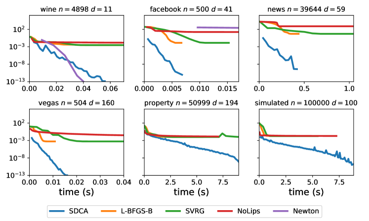
Figure 2: Convergence over time of five algorithms SDCA, SVRG, NoLips, L-BFGS-B and Newton on 6 datasets of Poisson regression. SDCA combines the best of both worlds: speed and scalability of SVRG and L-BFGS-B with the precision of Newton’s solution.

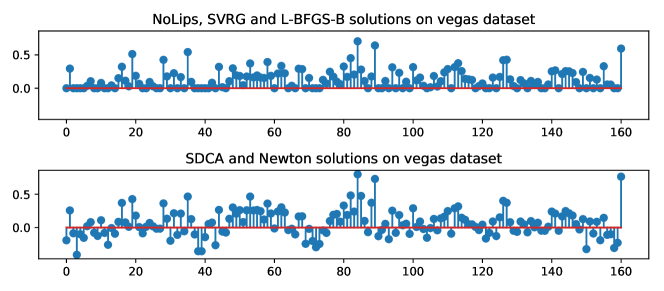
Figure 3: Estimated minimizers $w^{*}$ on the vegas dataset (160 features). The positive entries are roughly similarly recovered by all solvers but the negative entries are only retrieved by SDCA and Newton algorithms.

5.2 Hawkes processes

If the adjacency matrix $A$ is forced to be entrywise positive, then no event type can have an inhibitive effect on another. This ability to exhibit inhibitive effect has direct implications on real life datasets especially in finance where these effects are common [2, 3, 33]. In Figure 4 we present the aggregated influence of the kernels obtained after training a Hawkes process on a finance dataset exploring market microstructure [3]. While L-BFGS-B (or SVRG, or NoLips) recovers only excitation in the adjacency matrix, SDCA also retrieves inhibition that one event type might have on another.

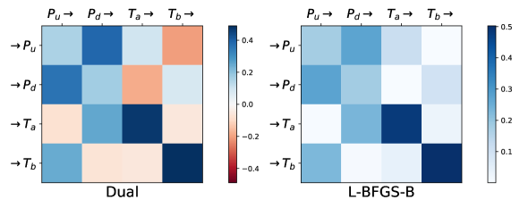
Figure 4: Adjacency matrix $A$ of a Hawkes process fitted on high-frequency financial data from the Bund market. This reproduces an experiment run in [3] where $P_{u}$ (resp. $P_{d}$) counts the number of upward (resp. downward) mid-price moves and $T_{a}$ (resp. $T_{b}$) counts the number of market orders at the best ask (resp. best bid) that do not move the price. SDCA detects inhibitive behaviors while L-BFGS-B cannot.

It is expected that when stocks are sold (resp. bought) the price is unlikely to go up (resp. down) but this is retrieved by SDCA only. On simulated data this is even clearer and in Figure 5 we observe the same behavior when the ground truth contains inhibitive effects. Our experiment consists in two simulated Hawkes processes with 10 nodes and sum-exponential kernels with 3 decays. There are only excitation effects - all $a^{ij}_{u}$ are positive - in the first case and we allow inhibitive effects in the second. Events are simulated according to these kernels that we try to recover. While it would be standard to compare the performances in terms of log-likelihood obtained on the a test sample, nothing ensures that the problem optimizer lies in the feasible set of the test set. Hence the results are compared by looking at the estimation error (RMSE) of the adjacency matrix $A$ across iterations. Figure 5 shows that SDCA always converges faster towards its solution in both cases and that when the adjacency matrix contains inhibitive effects, SDCA obtains a better estimation error than L-BFGS-B.

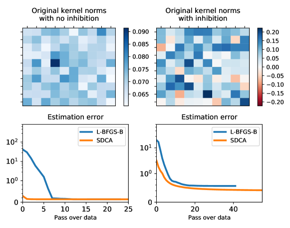
Figure 5: Top: Adjacency matrix of the Hawkes processes used for simulation. Bottom: estimation error of the adjacency matrix $A$ across iterations. In both case SDCA is faster than L-BFGS-B and reaches a better estimation error when there are inhibitive effects to recover (Right).

5.3 Heuristic initialization

The default dual initialization in [37] ($\alpha^{(0)}=0_{n}$) is not a feasible dual point. Instead of setting arbitrarily $\alpha^{(0)}$ to $1_{n}$, we design, from three properties, a vector $\kappa\in-\mathcal{D}_{f^{*}}^{n}$ that is linearly linked to $\alpha^{*}$ and then rely on Proposition 9 to find a heuristic starting point $\alpha^{(0)}$ from $\kappa$ for Poisson regression and Hawkes processes.

Property 1: link with $\|x_{i}\|$.

Proposition 8 relates exactly $\alpha_{i}^{*}$ to the inverse of the norm of $x_{i}$.

Proposition 8.

For Poisson regression and Hawkes processes, the value of the dual optimum $\alpha_{i}^{*}$ is linearly linked to the inverse of the norm of $x_{i}$. Namely, if there is $c_{i}>0$ such that $\xi_{i}=c_{i}x_{i}$ for any $i\in\{1,\dots n\}$, then $\zeta^{*}$, the solution of the dual problem

$$\operatorname*{arg\,max}_{\zeta\in(0,+\infty)^{n}}\frac{1}{n}\sum_{i=1}^{n}y_{i}+y_{i}\log\bigg{(}\frac{\zeta_{i}}{y_{i}}\bigg{)}-\lambda g^{*}\bigg{(}\frac{1}{\lambda n}\sum_{i=1}^{n}\zeta_{i}\xi_{i}-\frac{1}{\lambda}\psi\bigg{)},$$

satisfies $\zeta^{*}_{i}=\alpha_{i}^{*}/c_{i}$ for all $i=1,\dots n$.

This Proposition is proved in Section 7.12. It suggests to consider $\kappa_{i}\propto 1/\|x_{i}\|$ for all $i=1,\dots n$.

Property 2: link with $y_{i}$.

For Poisson regression and Hawkes processes where $f_{i}(x)=-y_{i}\log x$, the second Karush-Kuhn-Tucker Condition (14) (see Section 7.1 for more details) writes

$$\alpha_{i}^{*}=\frac{y_{i}}{{w^{*}}^{\top}x_{i}}$$

for $i=1,\dots,n$. Hence, $\alpha^{*}$ and $y$ are correlated (a change in $y_{i}$ only leads to a minor change in $w^{*}$), so we will consider $\kappa_{i}\propto y_{i}/\|x_{i}\|$.

Property 3: link with the features matrix.

The inner product ${w^{*}}^{\top}x_{i}$ is positive and at the optimum, the Karush-Kuhn-Tucker Condition (5) (which links $w^{*}$ to $x_{i}$ through $\alpha_{i}^{*}$) tells that $\alpha_{i}^{*}$ is likely to be large if $x_{i}$ is poorly correlated to other features, i.e. if $x_{i}^{\top}\sum_{j=1}^{n}x_{j}$ is small. Finally, the choice

$$\kappa_{i}=\frac{y_{i}}{x_{i}^{\top}\sum_{j=1}^{n}x_{j}}$$ (11)

for $i=1,\dots,n$, takes these three properties into account.

Figure 6 plots the optimal dual variables $\alpha^{*}$ from the Poisson regression experiments of Section 5.1 against the the $\kappa$ vector from Equation 11. We observe in these experiments a good correlation between the two, but $\kappa$ is only a good guess for initialization $\alpha^{(0)}$ up to a multiplicative factor that the following proposition aims to find.

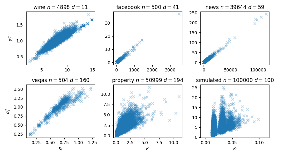
Figure 6: Value of $\alpha_{i}^{*}$ given $\kappa_{i}$ for $i=1,\ldots,n$. There is a linear link relating initial guess $\kappa_{i}$ to the dual optimum $\alpha_{i}^{*}$ on Poisson datasets but the amplitude is not adjusted yet.

Proposition 9.

For Poisson regression and Hawkes processes and $g(w)=\tfrac{1}{2}\|w\|^{2}$, if we constraint the dual solution ${\alpha^{*}\in(0,+\infty)^{n}}$ to be collinear with a given vector $\kappa\in(0,+\infty)^{n}$, i.e. $\alpha^{*}=\bar{\alpha}\kappa$ for some $\bar{\alpha}\in\mathbb{R},$ then the optimal value for $\bar{\alpha}$ is given by

$$\bar{\alpha}=\frac{\psi^{\top}\chi_{\kappa}+\sqrt{(\psi^{\top}\chi_{\kappa})^{2}+4\lambda\|\chi_{\kappa}\|^{2}\tfrac{1}{n}\sum_{i=1}^{n}y_{i}}}{2\|\chi_{\kappa}\|^{2}}\quad\text{with}\quad\chi_{\kappa}=\frac{1}{n}\sum_{i=1}^{n}\kappa_{i}x_{i}.$$

Combined with the previous Properties, we suggest to consider

$$\alpha^{(0)}_{i}=\bar{\alpha}\kappa_{i}$$ (12)

as an initial point, where $\kappa_{i}$ is defined in Equation (11).

This Proposition is proved in Section 7.13. Figure 7 presents the values of $\alpha_{i}^{*}$ given its initial value $\alpha_{i}^{(0)}$ for $i=1,\ldots,n$ and shows that the rescaling has worked properly. We validate this heuristic initialization by showing that it leads to a much faster convergence in Figure 8 below. Indeed, we observe that SDCA initialized with Equation (12) reaches optimal objective much faster than when initialization consists in setting all dual variables arbitrarily to 1.

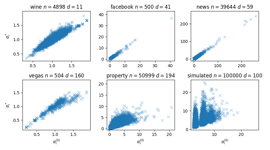
Figure 7: Value of $\alpha_{i}^{*}$ given $\alpha_{i}^{(0)}$ from Equation (12) for $i=1,\ldots,n$. These values are close an correlated which makes $\alpha^{(0)}$ a good initialization value.

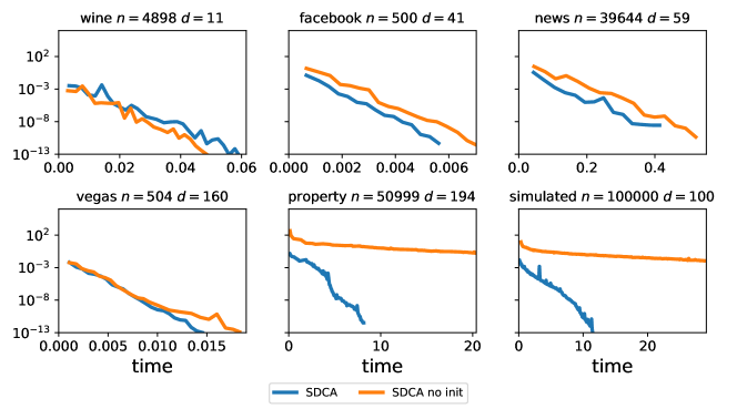
Figure 8: Convergence over time of SDCA with wise initialization from Equation (12) and SDCA arbitrarily initialized with $\alpha^{(0)}=1$.

5.4 Using mini batches

At each step $t$, SDCA [36] maximizes the dual objective by picking one index $i_{t}\in\{1,\dots,n\}$ and maximizing the dual objective over the coordinate $i_{t}$ of the dual vector $\alpha$, and sets

$$\alpha_{i}^{t+1}=\operatorname*{arg\,max}_{v\in-\mathcal{D}_{f^{*}}}D(\alpha_{1}^{t},\dots,\alpha_{i_{t}-1}^{t},v,\alpha_{i_{t}+1}^{t},\dots,\alpha_{n}).$$

In some cases this maximization has a closed-form solution, such as for Poisson regression (see Proposition 6) or least-squares regression where $f_{i}(w)=(y_{i}-w^{\top}x_{i})^{2}$ leads to the explicit update

$$\alpha_{i}^{t+1}=\alpha_{i}^{t}+\frac{y_{i}-w^{\top}x_{i}-\alpha_{i}^{t}}{1+(\lambda n)^{-1}\|x_{i}\|^{2}}.$$

In some other cases, such as logistic regression, this closed form solution cannot be exhibited and we must perform a Newton descent algorithm. Each Newton step consists in computing $\partial D(\alpha)/\partial\alpha_{i}$ and $\partial^{2}D(\alpha)/\partial\alpha_{i}^{2}$, which are one dimensional operations given $\|x_{i}\|^{2}$ and $w^{\top}x_{i}$. Hence, in a large dimensional setting, when the observations $x_{i}$ have many non zero entries, the main cost of the steps resides mostly in computing $\|x_{i}\|^{2}$ and $w^{\top}x_{i}$. Since $\|x_{i}\|^{2}$ and $w^{\top}x_{i}$ must also be computed when using a closed-form solution, using Newton steps instead of the closed-form is eventually not much more computationally expensive. So, in order to obtain a better trade-off between Newton steps and inner-products computations, we can consider more than a single index on which we maximize the dual objective. This is called the mini-batch approach, see Stochastic Dual Newton Ascent (SDNA) [32]. It consists in selecting a set $\mathcal{I}\subset\{1,\dots,n\}$ of $p$ indices at each iteration $t$. The value of $\alpha_{i}^{t+1}$ becomes in this case

$$\alpha_{i}^{t+1}=\operatorname*{arg\,max}_{v\in(-\mathcal{D}_{f^{*}})^{p}}D(b_{1},\dots,b_{n})\quad\text{where}\quad b_{i}=\begin{cases}v_{j}&\text{if}\quad i\in\mathcal{I}\text{ and }j\text{ is the position of }i\text{ in }\mathcal{I}\\ \alpha_{i}^{t}&\text{otherwise.}\end{cases}$$

The two extreme cases are $p=1$, which is the standard SDCA algorithm, and $p=n$ for which we perform a full Newton algorithm. After computing the inner products $w^{\top}x_{i}$ and $x_{i}^{\top}x_{j}$ for all $(i,j)\in\mathcal{I}^{2}$ each iteration will simply performs up to 10 Newton steps in which the bottleneck is to solve a $p\times p$ linear system. This allows to better exploit curvature and obtain better convergence guarantees for gradient-Lipschitz losses [32].

We can apply this to Poisson regression and Hawkes processes where $f_{i}(x)=-y_{i}\log x$. The maximization steps of Line 5 in Algorithm 2 is now performed on a set of coordinates $\mathcal{I}\subset\{1,\dots n\}$ and consists in finding

$$\max_{\alpha_{i};i\in\mathcal{I}}D_{\mathcal{I}}^{t}(\alpha_{\mathcal{I}})\quad\text{where}\quad D_{\mathcal{I}}^{t}(\alpha_{\mathcal{I}})=\frac{1}{n}\sum_{i\in\mathcal{I}}\Big{(}y_{i}+y_{i}\log\tfrac{\alpha_{i}}{y_{i}}\Big{)}-\frac{\lambda}{2}\Big{\|}w^{t}+\frac{1}{\lambda n}\sum_{i\in\mathcal{I}}(\alpha_{i}-\alpha_{i}^{t})x_{i}\Big{\|}^{2},$$

where we denote by $\alpha_{\mathcal{I}}$ the sub-vector of $\alpha$ of size $p$ containing the values of all indices in $\mathcal{I}$. We initialize the vector $\alpha_{\mathcal{I}}^{(0)}\in(-\mathcal{D}_{f^{*}})^{p}$ to the corresponding values of the coordinates of $\alpha^{t}$ in $\mathcal{I}$ and then perform the Newton steps, i.e.

$$\alpha_{\mathcal{I}}^{k+1}=\alpha_{\mathcal{I}}^{k}-\Delta\alpha_{\mathcal{I}}^{k}\quad\text{where }\Delta\alpha_{I}^{k}\text{ is the solution of}\quad\nabla^{2}D_{\mathcal{I}}^{t}(\alpha_{\mathcal{I}}^{k})\Delta\alpha_{\mathcal{I}}^{k}=\nabla D_{\mathcal{I}}^{t}(\alpha_{\mathcal{I}}^{k}).$$ (13)

The gradient $\nabla D_{\mathcal{I}}^{t}(\alpha_{\mathcal{I}}^{k})$ and the hessian $\nabla^{2}D_{\mathcal{I}}^{t}(\alpha_{\mathcal{I}}^{k})$ have the following explicit formulas:

$$(\nabla D_{\mathcal{I}}^{t}(\alpha_{\mathcal{I}}^{k}))_{i}=\frac{\partial D(\alpha_{\mathcal{I}}^{k})}{\partial\alpha_{i}}=\frac{1}{n}\Big{(}\frac{y_{i}}{\alpha_{i}^{k}}-{w^{t}}^{\top}x_{i}-\frac{1}{\lambda n}\sum_{j\in\mathcal{I}}(\alpha_{j}^{k}-\alpha_{j}^{t})x_{j}^{\top}x_{i}\Big{)},$$

and

$$\big{(}\nabla^{2}D_{I}^{t}(\alpha_{I}^{k})\big{)}_{i,j}=\frac{\partial^{2}D(\alpha_{I}^{k})}{\partial\alpha_{i}\partial\alpha_{j}}=-\frac{1}{n}\Big{(}\frac{y_{i}}{{\alpha_{i}^{k}}^{2}}\mathbf{1}_{i=j}+\frac{1}{\lambda n}x_{i}^{\top}x_{j}\Big{)}.$$

Note that $D_{I}^{t}$ is a concave function hence $-\nabla^{2}D_{I}^{t}(\alpha_{I}^{k})$ will be positive semi-definite and the system in Equation (13) can be solved very efficiently with BLAS and LAPACK libraries. Let us explicit computations when $p=2$. Suppose that $\mathcal{I}=\{i,j\}$ and put

$$\delta_{i}=\alpha_{i}-\alpha_{i}^{(t-1)},\quad p_{i}=x_{i}^{\top}w^{(t-1)}\quad\text{and}\quad g_{ij}=\frac{x_{i}^{\top}x_{j}}{\lambda n}.$$

The gradient and the Hessian inverse are then given by

$$\nabla D(\alpha_{I})=\frac{1}{n}\begin{bmatrix}\frac{y_{i}}{\alpha_{i}}-p_{i}-\delta_{i}g_{ii}-\delta_{j}g_{ij}\\ \frac{y_{j}}{\alpha_{j}}-p_{j}-\delta_{j}g_{jj}-\delta_{i}g_{ij}\end{bmatrix},$$

and

$$\nabla^{2}D(\alpha_{I})^{-1}=\frac{n^{2}}{(\frac{y_{i}}{\alpha_{i}^{2}}+g_{ii})(\frac{y_{i}}{\alpha_{i}^{2}}+g_{ii})-g_{ij}^{2}}\begin{bmatrix}-\frac{y_{j}}{\alpha_{j}^{2}}-g_{jj}&g_{ij}\\ g_{ij}&-\frac{y_{i}}{\alpha_{i}^{2}}-g_{ii}\end{bmatrix}.$$

This direct computation leads to even faster computations than using the dedicated libraries. We plot in Figure 9 the convergence speed for three sizes of batches 1, 2 and 10. Note that in all cases using a batch of size $p=2$ is faster than standard SDCA. Also, in the last simulated experiment where $d$ has been set on purpose to $1000$, the solver using batches of size $p=10$ is the fastest one. The bigger number of features $d$ gets, the better are solvers using big batches.

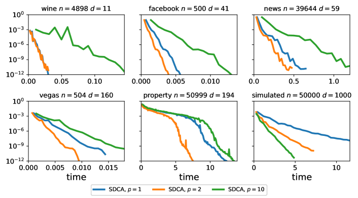
Figure 9: Convergence speed comparison when the number of indices optimized at each step changes.

5.5 About the pessimistic upper bounds

The generic upper bounds derived in Proposition 7 are general but pessimistic as they depend linearly on $n$. In fact this dependence is also observed in the NoLips algorithm [4] where the rate depends on a constant $L=\sum_{i}^{n}y_{i}$. Note that, for Nolips algorithms, $L$ is involved in the step size definition and leads to step too small to be used in practice but that in our algorithm, these bounds have little or even no impact in practice (see Remark 2) and are mainly necessary for convergence guarantees. These bounds are derived by lower bounding $x_{i}^{\top}\sum_{j\neq i}\alpha_{j}^{*}x_{j}$ by $0$. This lower bound is very conservative and can probably be tightened by setting specific hypotheses on the dataset, for example on the Gram matrix ($[G]_{i,j}=x_{i}^{\top}x_{j}$ for $i,j=1,\ldots,n$). For Poisson regression, this lower bound is reached in the extreme case where all observations are orthogonal (all entries of $G$ are zero except on the diagonal). Then $\psi^{\top}x_{i}=\frac{1}{n}\|x_{i}\|^{2}$ and the upper bounds from Proposition 7 become

$$\beta_{i}=\frac{1}{2}+\sqrt{\frac{1}{4}+\frac{\lambda ny_{i}}{\|x_{i}\|^{2}}}$$

for $i=1,\ldots,n$. In this extreme case, the bounds are $O(\sqrt{n})$ instead of $O(n)$ as stated in Proposition 7. Experimentally, we do not observe a dependence in $O(n)$ either. Figure 10 shows the evolution of the maximum optimal dual obtained ($\max_{i=1,\ldots,n}\alpha_{i}^{*}$) for the six datasets considered in Section 5.1 for Poisson regression, on an increasing fraction of the dataset. These values are averaged over 20 samples and we provide the associated 95% confidence interval on this value. We observe that $\max_{i=1,\ldots,n}\alpha_{i}^{*}$ has a much lower dependence in $n$ than the bounds given by Proposition 7.

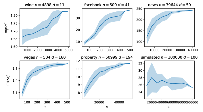
Figure 10: Evolution of $\max_{i=1,\ldots,n}\alpha_{i}^{*}$ for an increasing value of $n$. We observe that $\max_{i=1,\ldots,n}\alpha_{i}^{*}$ is not increasing linearly with $n$ as quick as the bound $\beta_{i}$ obtained in Proposition 7.

6 Conclusion

This work introduces the $\log$-smoothness assumption in order to derive improved linear rates for SDCA, for objectives that do not meet the gradient-Lipschitz assumption. This provides, to the best of our knowledge, the first linear rates for a stochastic first order algorithm without the gradient-Lipschitz assumption. The experimental results also prove the efficiency of SDCA to solve such problems and its ability to deal with the open polytope constraints, improving the state-of-the-art. Finally, this work also presents several variants of SDCA and experimental heuristics to make the most of it on real world datasets. Future work could provide better linear rates under more specialized assumptions on the Gram matrix, as observed on numerical experiments. Also, to extend this work to more applications, we aim to find a generalization of the $\log$ smoothness assumption such as what [38] has done for self-concordance.

Acknowledgments

We would like to acknowledge support for this project from the Datascience Initiative of École polytechnique

7 Proofs

We start this Section by providing extra details on the derivation of the dual problem and the proximal version of SDCA. We then provides the proofs of all the results stated in the chapter, namely Proposition 2, Proposition 3, Theorem 4, Theorem 5, Proposition 6, Proposition 7, Remark 2, Proposition 8 and Proposition 9.

7.1 Duality and proof of Proposition 1

It is not straightforward to obtain strong duality for a convex problem with strict inequalities (such as the ones enforced by the polytope $\Pi(X)$ from Equation 3). To bypass this difficulty we consider the same problem but constrained on a closed set and show how it relates to the original Problem (2). But first we formulate the two following lemmas.

Lemma 10.

It exists $\varepsilon>0$ such that the following problem

$$\min_{w\in\Pi_{|\varepsilon}(X)}P(w)\quad\text{where}\quad\Pi_{|\varepsilon}(X)=\{w\in\mathbb{R}^{d}\;:\;\forall i\in\{1,\dots,n\},\;w^{\top}x_{i}\geq\varepsilon\}$$

has a solution $w^{*}$ that is also the solution of the original Problem (2).

Proof.

First, notice that this problem has a unique solution which is unique as we minimize a convex function on a closed convex set $\Pi(X)$. Also, as the function $w\mapsto\psi^{\top}w+\lambda g(w)$ is strongly convex, since $g$ is strongly convex, it is lower bounded. We denote by $M\in\mathbb{R}$ a lower bound of this function. Then, we consider $w^{0}\in\Pi(X)$, and choose $\varepsilon$ sufficiently small such that for all $i=1,\dots,n$,

$$\forall t<\varepsilon,\;f_{i}(t)>nP(w^{0})-nM,$$

this value of $\varepsilon$ always exists since by assumption $\lim_{t\rightarrow 0}f_{i}(t)=+\infty$ for all $i=1,\dots,n$. For any $w_{\varepsilon}\in\Pi(X)\setminus\Pi_{\varepsilon}(X)$ (so a $w_{\varepsilon}$ is such that $\exists i\in\{1,\dots,n\},\;w_{\varepsilon}^{\top}x_{i}<\varepsilon$), we thus have

$$P(w_{\varepsilon})>\psi^{\top}w_{\varepsilon}+P(w^{0})-M+\lambda g(w_{\varepsilon})\geq P(w^{0}).$$

Hence, for such a value of $\varepsilon$, the solution to the original Problem (2) is necessarily in $\Pi_{\varepsilon}(X)$ and both the problems constrained on $\Pi_{\varepsilon}(X)$ and $\Pi(X)$ share the same solution $w^{*}$. ∎

Lemma 11.

For all $i=1,\dots,n$, if we define by

$$\forall\alpha_{i}\in\mathcal{D}_{f^{*}},\;f^{*}_{i|\varepsilon}(v):=\max_{u\geq\varepsilon}uv-f_{i}(u),$$

then $f^{*}_{i|\varepsilon}$ is equal to the Fenchel conjugate of $f_{i}$, $f_{i}^{*}$, on $\{v\;;\;\exists u\geq\varepsilon\;;\;v=f_{i}^{\prime}(u)\}$.

Proof.

For all $i=1,\dots,n$, the functions $f_{i}$ are convex and differentiable. Hence, by Fermat’s rule if $\exists u^{*}\geq\varepsilon;\;v=f_{i}^{\prime}(u^{*})$ then $f^{*}_{i|\varepsilon}(v)=\max_{u\geq\varepsilon}uv-f_{i}(u)=u^{*}f_{i}^{\prime}(u^{*})-f_{i}(u^{*})$. Likewise, the maximization step in the computation of $f_{i}^{*}$ would share the same maximizer and ${f_{i}^{*}}(v)=u^{*}f_{i}^{\prime}(u^{*})-f_{i}(u^{*})$ as well. Hence,

$$\forall v\;\text{such that}\;\exists u\geq\varepsilon\;;\;v=f_{i}^{\prime}(u);\;f^{*}_{i|\varepsilon}(v)={f_{i}^{*}}(v).$$

∎

We form the dual of the problem constrained on $\Pi_{\varepsilon}(X)$ where $\varepsilon$ is such that Lemma 10 applies. We replace the inner products $w^{\top}x_{i}$ by the scalars $u_{i}$ for $i=1,\ldots,n$ and their equality is constrained to form the strictly equivalent problem:

$$\min_{\begin{subarray}{c}w\in\mathbb{R}^{d},u\in{[\varepsilon,+\infty)}^{n}\\ \forall i,u_{i}=w^{\top}x_{i}\end{subarray}}\psi^{\top}w+\frac{1}{n}\sum_{i=1}^{n}f_{i}(u_{i})+\lambda g(w).$$

We maximize the Lagrangian to include the constraints. This introduces the vector of dual variables $\alpha\in\mathbb{R}^{n}$ as following:

$$\max_{\alpha\in\mathbb{R}^{n}}\min_{\begin{subarray}{c}w\in\mathbb{R}^{d}\\ u\in{[\varepsilon,+\infty)}^{n}\end{subarray}}\psi^{\top}w+\frac{1}{n}\sum_{i=1}^{n}f_{i}(u_{i})+\lambda g(w)+\frac{1}{n}\sum_{i=1}^{n}\alpha_{i}(u_{i}-x_{i}^{\top}w)$$

that leads to the corresponding dual problem:

$$\max_{\alpha\in(-\mathcal{D}_{f^{*}_{|\varepsilon}})^{n}}D_{|\varepsilon}(\alpha),\quad D_{|\varepsilon}(\alpha)=\frac{1}{n}\sum_{i=1}^{n}-f^{*}_{i|\varepsilon}(-\alpha_{i})-\lambda g^{*}\bigg{(}\frac{1}{\lambda n}\sum_{i=1}^{n}\alpha_{i}x_{i}-\frac{1}{\lambda}\psi\bigg{)},$$

where $-\mathcal{D}_{f^{*}_{|\varepsilon}}$ is the domain of all $f^{*}_{i|\varepsilon}$. The primal problem constrained on $\Pi_{\varepsilon}(X)$ verifies the Slater’s conditions so strong duality holds and the maximizer of $D_{|\varepsilon}$, $\alpha^{*}_{|\varepsilon}$, is reached. As $D_{|\varepsilon}$ is concave, $\alpha^{*}_{|\varepsilon}$ is the only vector such that $\nabla D_{|\varepsilon}(\alpha^{*}_{|\varepsilon})=0$. Also, as strong duality holds, we can relate $\alpha^{*}_{|\varepsilon}$ to the primal optimum though the Karush-Kuhn-Tucker condition

$$\alpha^{*}_{i|\varepsilon}=-{f^{*}_{i|\varepsilon}}^{\prime}({w^{*}}^{\top}x_{i}),$$

where $w^{*}$ is such that ${w^{*}}^{\top}x_{i}\geq\varepsilon$ (see Lemma 10). Hence Lemma 11 applies and the dual formulation of the original Problem (2) that writes

$$\max_{\alpha\in(-\mathcal{D}_{f^{*}})^{n}}D(\alpha),\quad D(\alpha)=\frac{1}{n}\sum_{i=1}^{n}-f_{i}^{*}(-\alpha_{i})-\lambda g^{*}\bigg{(}\frac{1}{\lambda n}\sum_{i=1}^{n}\alpha_{i}x_{i}-\frac{1}{\lambda}\psi\bigg{)},$$

is such that $\nabla D(\alpha^{*}_{|\varepsilon})=\nabla D_{|\varepsilon}(\alpha^{*}_{|\varepsilon})=0$. Since $D(\alpha)$ is concave, this means that $\alpha^{*}_{|\varepsilon}=\alpha^{*}$ where $\alpha^{*}$ is the solution of the dual formulation of the original Problem (2). Thus, the Karush-Kuhn-Tucker conditions that link the primal and dual optima of the problem constrained on $\Pi_{|\varepsilon}(X)$ also links the primal and dual optima of the original Problem (2). The first one is given in Equation (5) and the second one writes

$$\alpha_{i}^{*}=-{f_{i}^{*}}^{\prime}({w^{*}}^{\top}x_{i})$$ (14)

for any $i\in\{1,\dots n\}$. From the first we can define two functions linking vector $w\in\mathbb{R}^{d}$ to $\alpha\in(-\mathcal{D}_{f^{*}})^{n}$ and such that $w(\alpha^{*})=w^{*}$ and

$$v(\alpha)=\frac{1}{\lambda n}\sum_{i=1}^{n}\alpha_{i}x_{i}-\frac{1}{\lambda}\psi\quad\text{and}\quad w(\alpha)=\nabla g^{*}\big{(}v(\alpha)\big{)}.$$ (15)

7.2 Proximal algorithm

Given that $g^{*}$ is smooth since its Fenchel conjugate is strongly convex, the gradient-Lipschitz property from Definition 4 below entails $g^{*}(v+\Delta v)\leq g^{*}(v)+\nabla g^{*}(v)^{\top}\Delta v+\tfrac{1}{2}\|\Delta v\|^{2}$. Hence, maximization step of Algorithm 1, namely,

$$\operatorname*{arg\,max}_{\alpha_{i}\in-\mathcal{D}_{f^{*}}}-f^{*}_{i}(-\alpha_{i})-\lambda ng^{*}\big{(}v^{(t-1)}+(\lambda n)^{-1}(\alpha_{i}-\alpha_{i}^{(t-1)})x_{i}\big{)},$$

where $v^{(t-1)}=\frac{1}{\lambda n}\sum_{i=1}^{n}\alpha_{i}^{(t-1)}x_{i}-\frac{1}{\lambda}\psi$ can be simplified by setting $\alpha_{i}^{t}$ such that it maximizes the lower bound

$$\alpha_{i}^{t}=\operatorname*{arg\,max}_{\alpha_{i}\in-\mathcal{D}_{f^{*}}}-f^{*}_{i}(-\alpha_{i})-\lambda n\bigg{(}g^{*}\big{(}v^{(t-1)}\big{)}+\frac{\alpha_{i}-\alpha_{i}^{(t-1)}}{\lambda n}x_{i}^{\top}\nabla g^{*}(v^{(t-1)})+\frac{1}{2}\bigg{(}\frac{\alpha_{i}-\alpha_{i}^{(t-1)}}{\lambda n}\bigg{)}^{2}\|x_{i}\|^{2}\bigg{)}.$$ (16)

Setting $w^{(t-1)}=\nabla g^{*}(v^{(t-1)})$ and discarding constants terms leads to the equivalent relation,

$$\alpha_{i}^{t}=\operatorname*{arg\,max}_{\alpha_{i}\in-\mathcal{D}_{f^{*}}}-f^{*}_{i}(-\alpha_{i})-\frac{\lambda n}{2}\Big{\|}w^{(t-1)}-(\lambda n)^{-1}(\alpha_{i}-\alpha_{i}^{(t-1)})x_{i}\Big{\|}^{2}.$$

While convergence speed is guaranteed for any 1-strongly convex $g$, to simplify the algorithm we will consider that $g$ is not only 1-strongly convex but that that it can also be decomposed as

$$g(w)=\tfrac{1}{2}\|w\|^{2}+h(w)$$

where $h$ is a prox capable function. With Proposition 12 below the relation between $w^{t}$ and $v^{t}$ becomes

$$w^{t}=\nabla g^{*}(v^{t})=\operatorname*{arg\,sup}_{u\in\mathbb{R}^{d}}\Big{(}u^{\top}v^{t}-\tfrac{1}{2}\|u\|^{2}-h(u)\Big{)}=\operatorname*{arg\,inf}_{u\in\mathbb{R}^{d}}\Big{(}\tfrac{1}{2}\|v^{t}-u\|^{2}+h(u)\Big{)},$$

which is the proximal operator stated in Definition 6 below: $w^{t}=\operatorname{prox}_{h}(v(\alpha^{t}))$.

7.3 Preliminaries for the proofs

Let us first recall some definitions and basic properties.

Definition 3.

Strong convexity. A differentiable convex function $f:\mathcal{D}_{f}\rightarrow\mathbb{R}$ is $\gamma$-strongly convex if

$$\forall x,y\in\mathcal{D}_{f},\quad f(y)\geq f(x)+f^{\prime}(x)^{\top}(y-x)+\frac{\gamma}{2}\|y-x\|^{2}.$$ (17)

This is equivalent to

$$\forall x,y\in\mathcal{D}_{f},\quad(f^{\prime}(y)-f^{\prime}(x))(y-x)\geq\gamma\|y-x\|^{2}.$$ (18)

Definition 4.

Smoothness. A differentiable convex function $f:\mathcal{D}_{f}\rightarrow\mathbb{R}$ is $L$-smooth or $L$-gradient Lipschitz if

$$\forall x,y\in\mathcal{D}_{f},\quad f(y)\leq f(x)+f^{\prime}(x)(y-x)+\frac{L}{2}\|y-x\|^{2}.$$

This is equivalent to

$$\forall x,y\in\mathcal{D}_{f},\quad(f^{\prime}(y)-f^{\prime}(x))(y-x)\leq L\|y-x\|^{2}.$$

Definition 5.

Fenchel conjugate. For a convex function $f:\mathcal{D}_{f}\rightarrow\mathbb{R}$ we call Fenchel conjugate the function $f^{*}$ defined by

$$f^{*}:\mathcal{D}_{f^{*}}\rightarrow\mathbb{R},\quad\text{st.}\quad f^{*}(v)=\sup_{u\in\mathcal{D}_{f}}\big{(}u^{\top}v-f(u)\big{)}.$$ (19)

Proposition 12.

For a convex differentiable function $f$, the gradient of its differentiable Fenchel conjugate $f^{*}$ is the maximizing argument of (19):

$${f^{*}}^{\prime}(v)=\operatorname*{arg\,sup}_{u\in\mathcal{D}_{f}}\big{(}u^{\top}v-f(u)\big{)}.$$

Proposition 13.

For a convex differentiable function $f$ and its differentiable Fenchel conjugate $f^{*}$ we have

$$\forall u\in\mathcal{D}_{f},{f^{*}}^{\prime}(f^{\prime}(u))=u\quad\text{and}\quad\forall v\in\mathcal{D}_{f^{*}},f^{\prime}({f^{*}}^{\prime}(v))=v.$$

This leads to

$$\forall u\in\mathcal{D}_{f},\forall v\in\mathcal{D}_{f^{*}},\quad f^{\prime}(u)=v\Leftrightarrow u={f^{*}}^{\prime}(v).$$

Note that if $f$ is $\gamma$-strongly convex (respectively $L$-smooth), then its Fenchel conjugate $f^{*}$ is $1/\gamma$ smooth (respectively $1/L$ strongly convex). We also recall results from [27] on self-concordant functions introduced in Definition 2. This concept is widely used to study losses involving logarithms. For the sake of clarity, the results will be presented for functions whose domain $\mathcal{D}_{f}$ is a subset of $\mathbb{R}$ as this leads to lighter notations. Unlike smoothness and strong convexity, this property is affine invariant. From this definition, some inequalities are derived in [27]. Two of them provide lower bounds that are comparable to strong convexity inequalities:

$$\forall x,y\in\mathcal{D}_{f},\quad f(y)\geq f(x)+f^{\prime}(x)(y-x)+\omega\big{(}\sqrt{f^{\prime\prime}(x)}|y-x|\big{)}$$ (20)

where $\omega(t)=t-\log(1+t)$, and

$$\forall x,y\in\mathcal{D}_{f},\quad(f^{\prime}(y)-f^{\prime}(x))^{\top}(y-x)\geq\frac{f^{\prime\prime}(x)(y-x)^{2}}{1+\sqrt{f^{\prime\prime}(x)}|y-x|}.$$ (21)

Finally, we define the proximal operator used to apply the penalization $g$.

Definition 6.

Proximal operator. For a convex function $g:\mathcal{D}_{g}\rightarrow\mathbb{R}$, the proximal operator associated to $g$ is given by

$$\operatorname{prox}_{g}(y)=\operatorname*{arg\,min}_{x\in\mathcal{D}_{g}}\Big{(}\frac{1}{2}\|y-x\|^{2}+g(x)\Big{)}.$$

The proximal operator always exists and is uniquely defined as the minimizer of a strongly convex function. Before the proof of Theorem 4, we need to introduce new convex inequalities for $L$-$\log$ smooth functions. This class of function includes $x\mapsto-L\log x$ which is our function of interest in the Poisson and in the Hawkes cases.

7.4 Proof of Proposition 2

First order implies second order

We start by showing that if $f$ is a L $\log$-smooth function then we can bound its second derivative by the square of its gradient. For any $x\in\mathcal{D}_{f}$, we set $y=x+h$ in the Definition 1, which now writes

$$\forall x\in\mathcal{D}_{f},\;\forall h\text{ s.t. }(x+h)\in\mathcal{D}_{f},\;\Big{|}\frac{f^{\prime}(x)-f^{\prime}(x+h)}{h}\Big{|}\leq\frac{1}{L}f^{\prime}(x)f^{\prime}(x+h).$$

Taking the limit of the previous inequality when $h$ tends towards $0$ leads to the desired inequality,

$$\forall x\in\mathcal{D}_{f},\;\big{|}f^{\prime\prime}(x)\big{|}\leq\frac{1}{L}f^{\prime}(x)^{2}.$$

Second order implies first order

We now prove that if $f$ is convex strictly monotone, twice differentiable and $|f^{\prime\prime}(x)|\leq\frac{1}{L}f^{\prime}(x)^{2}$ then $f$ is $L$-$\log$ smooth. If for all $x\in\mathcal{D}_{f}$, we denote by $\phi:x\mapsto\frac{1}{f^{\prime}(x)}$, (note that $\forall x\in\mathcal{D}_{f},f^{\prime}(x)\neq 0$ as $f$ is strictly monotone), then

$$\forall x\in\mathcal{D}_{f},\;|\phi^{\prime}(x)|=\Big{|}\frac{f^{\prime\prime}(x)}{f^{\prime}(x)^{2}}\Big{|}\leq\frac{1}{L}.$$

From this inequality, we limit the increasings of the function $\phi$,

$$\forall x,y\in\mathcal{D}_{f},\;-\tfrac{1}{L}|y-x|\leq\phi(y)-\phi(x)\leq\tfrac{1}{L}|y-x|,$$

which rewrites

$$\forall x,y\in\mathcal{D}_{f},\;|\phi(y)-\phi(x)|\leq\tfrac{1}{L}|y-x|\;\Leftrightarrow\;\Big{|}\frac{f^{\prime}(x)-f^{\prime}(y)}{f^{\prime}(x)f^{\prime}(y)}\Big{|}\leq\frac{1}{L}|x-y|,$$

that is the definition of a $L$-$\log$ smooth function for a convex strictly monotone function.

7.5 Proof of Proposition 3

We working by exhibiting several statements equivalent to $\log$ smoothness. First, we divide both sides of the $\log$ smoothness definition by $f^{\prime}(x)f^{\prime}(y)>0$ since $f$ is strictly monotone,

$$\text{$f$ is $L$-$\log$ smooth}\quad\Leftrightarrow\quad\forall x,y\in\mathcal{D}_{f},\;\bigg{|}\frac{1}{f^{\prime}(y)}-\frac{1}{f^{\prime}(x)}\bigg{|}\leq\frac{1}{L}|x-y|.$$

Then we rewrite the equation in the dual space using Proposition 13,

$$\text{$f$ is $L$-$\log$ smooth}\quad\Leftrightarrow\quad\forall x,y\in\mathcal{D}_{f^{*}},\;\bigg{|}\frac{1}{y}-\frac{1}{x}\bigg{|}\leq\frac{1}{L}|{f^{*}}^{\prime}(x)-{f^{*}}^{\prime}(y)|.$$

This can be rewritten into the following integrated form

$$\text{$f$ is $L$-$\log$ smooth}\quad\Leftrightarrow\quad\forall x,y\in\mathcal{D}_{f^{*}},\;\Big{|}\int_{y}^{x}t^{-2}dt\Big{|}\leq\frac{1}{L}\Big{|}\int_{y}^{x}({f^{*}}^{\prime\prime}(t)dt\Big{|},$$

which becomes equivalent to the desired result with the fundamental theorem of calculus

$$\text{$f$ is $L$-$\log$ smooth}\quad\Leftrightarrow\quad\forall x\in\mathcal{D}_{f^{*}},\;x^{-2}\leq\frac{1}{L}{f^{*}}^{\prime\prime}(x).$$

7.6 Inequalities for log-smooth functions

The proof of SDCA [36] relies on the smoothness of the functions $f_{i}$ which implies strong convexity of their Fenchel conjugates $f_{i}^{*}$. Indeed, a $\gamma$ strongly convex function $f^{*}$ satisfies the following inequality

$$sf^{*}(x)+(1-s)f^{*}(y)\geq f^{*}(sx+(1-s)y)+\frac{\gamma}{2}s(1-s)(y-x)^{2}.$$ (22)

This inequality is not satisfied for $L$-$\log$ smooth functions. However, we can derive for such functions another inequality which can be compared to such inequalities based on self-concordance and strongly convex properties.

Lemma 14.

Let $f:\mathcal{D}_{f}\subset\mathbb{R}\rightarrow\mathbb{R}$ be a strictly monotone convex function and $f^{*}$ be its differentiable Fenchel conjugate. Then,

$$\text{$f$ is $L$-$\log$ smooth}\quad\Leftrightarrow\quad\forall x,y\in\mathcal{D}_{f^{*}},\;({f^{*}}^{\prime}(x)-{f^{*}}^{\prime}(y))(x-y)\geq L\frac{(x-y)^{2}}{xy}.$$

This bound is an equality for $f(x)=-L\log x$.

Proof.

From $\log$ smoothness definition, we obtain by multiplying both sides by $|f^{\prime}(x)-f^{\prime}(y)|$ and dividing by $f^{\prime}(x)f^{\prime}(y)>0$ (since $f$ is strictly monotone),

$$\text{$f$ is $L$-$\log$ smooth}\quad\Leftrightarrow\quad\forall x,y\in\mathcal{D}_{f},\;\frac{\big{(}f^{\prime}(x)-f^{\prime}(y)\big{)}^{2}}{f^{\prime}(x)f^{\prime}(y)}\leq\frac{1}{L}|x-y||f^{\prime}(x)-f^{\prime}(y)|$$

Since $f$ is a convex function, $(f^{\prime}(x)-f^{\prime}(y))(x-y)\geq 0$ and using Proposition  13, we can rewrite the previous equivalence in the dual space:

$$\text{$f$ is $L$-$\log$ smooth}\quad\Leftrightarrow\quad\forall x,y\in\mathcal{D}_{f^{*}},\;\frac{(x-y)^{2}}{xy}\leq\frac{1}{L}({f^{*}}^{\prime}(x)-{f^{*}}^{\prime}(y))(x-y),$$

which concludes the proof. ∎

Lemma 15.

Let $f:\mathcal{D}_{f}\subset\mathbb{R}\rightarrow\mathbb{R}$ be a strictly monotone convex function and $f^{*}$ be its differentiable Fenchel conjugate. Then,

$$\text{$f$ is $L$-$\log$ smooth}\quad\Leftrightarrow\quad\forall x,y\in\mathcal{D}_{f^{*}},\;{f^{*}}(x)-{f^{*}}(y)-{f^{*}}^{\prime}(y)(x-y)\geq L\Big{(}\frac{x}{y}-1-\log\frac{x}{y}\Big{)}.$$

This bound is an equality for $f(x)=-L\log x$.

Proof.

Let $x,y\in\mathcal{D}_{f^{*}}$, we have the following on the one hand,

$${f^{*}}(x)-{f^{*}}(y)-{f^{*}}^{\prime}(y)(x-y)=\int_{y}^{x}\big{(}{f^{*}}^{\prime}(u)-{f^{*}}^{\prime}(y)\big{)}\mathop{}\!\mathrm{d}u$$

On the other hand, applying Lemma 14 together with the fundamental theorem of calculus gives

$$\text{$f$ is $L$-$\log$ smooth}\quad\Leftrightarrow\quad\forall x,y\in\mathcal{D}_{f^{*}},\;\int_{y}^{x}({f^{*}}^{\prime}(u)-{f^{*}}^{\prime}(y))\mathop{}\!\mathrm{d}u\geq\int_{y}^{x}L\;\frac{u-y}{uy}\mathop{}\!\mathrm{d}u.$$

Finally, solving the integral leads to the desired result:

$$\forall x,y\in\mathcal{D}_{f^{*}},\;\int_{y}^{x}L\;\frac{u-y}{uy}\mathop{}\!\mathrm{d}u=L\int_{y}^{x}\bigg{(}\frac{1}{y}-\frac{1}{u}\bigg{)}\mathop{}\!\mathrm{d}u=L\bigg{(}\frac{x-y}{y}-\log\frac{x}{y}\bigg{)}.$$

∎

Lemma 16.

Assume that $f$ is $L$-$\log$ smooth and $f^{*}$ is its differentiable Fenchel conjugate, then,

$$s{f^{*}}(x)+(1-s){f^{*}}(y)-{f^{*}}(y+s(x-y))\geq L\bigg{(}\log\Big{(}1-s+s\frac{x}{y}\Big{)}-s\log\frac{x}{y}\bigg{)}$$

for any $y,x\in\mathcal{D}_{f^{*}}$ and $s\in[0,1]$. This bound is an equality for $f(x)=-L\log x$.

Proof.

Let $x,y\in\mathcal{D}_{f^{*}}$ and define for any $s\in[0,1]$, $u(s)=sx+(1-s)y$. We apply Lemma 15 twice for $x$, $u(s)$ and $y$, $u(s)$:

$$f^{*}(x)-f^{*}(u(s))-{f^{*}}^{\prime}(u(s))(x-u(s))\geq L\Big{(}\frac{x}{u(s)}-1-\log\frac{x}{u(s)}\Big{)},$$ (23)

$$f^{*}(y)-f^{*}(u(s))-{f^{*}}^{\prime}(u(s))(y-u(s))\geq L\Big{(}\frac{y}{u(s)}-1-\log\frac{y}{u(s)}\Big{)}.$$ (24)

Combining $s$(23) and $(1-s)$(24) leads to

$$sf^{*}(x)+(1-s)f^{*}(y)-f^{*}(u(s)) \geq-sL\log\frac{x}{u(s)}-(1-s)L\log\frac{y}{u(s)}$$

$$\qquad+L\bigg{(}s\frac{x}{u(s)}+(1-s)\frac{y}{u(s)}-1\bigg{)}$$

$$=sL\log\frac{u(s)}{x}+(1-s)L\log\frac{u(s)}{y}$$

$$=sL\log\frac{u(s)}{y}+sL\log\frac{y}{x}+(1-s)L\log\frac{u(s)}{y}$$

$$=L\log\Big{(}1-s+s\frac{x}{y}\Big{)}+sL\log\frac{y}{x}.\qed$$

This Lemma which implies the barycenter $u(s)=y+s(x-y)$ for $s\in[0,1]$ is the lower bound that we actually use in proof of Theorem 4. To compare this result with strong convexity and self-concordance assumptions, we will suppose that $f^{*}$ is twice differentiable and hence that Proposition 3 applies.

Comparison with self-concordant functions

Instead of building our lower bounds on $\log$ smoothness, we rather exhibit what can be obtained with self-concordance combined with the lower bound ${{f^{*}}^{\prime\prime}(y)\geq Ly^{-2}}$ from Proposition 3. In this paragraph, we consider that $\frac{1}{L}f^{*}$ is standard self-concordant, such an hypothesis is verified for $f:t\mapsto-\frac{1}{L}\log(t)$. Hence, using lower bound (21) on $\frac{1}{L}f$ and then Proposition 3, we obtain

$$\forall x,y\in\mathcal{D}_{f^{*}},~{}({f^{*}}^{\prime}(x)-{f^{*}}^{\prime}(y))(x-y)\geq\frac{{f^{*}}^{\prime\prime}(y)(x-y)^{2}}{1+\sqrt{\frac{1}{L}{f^{*}}^{\prime\prime}(y)}|x-y|}\geq L\frac{(x-y)^{2}}{y^{2}+|y(x-y)|}.$$

Since $\forall x,y\in\mathcal{D}_{f^{*}}$, $xy>0$, this lower bound is equivalent to Lemma 14 if $|x|\geq|y|$ but not as good otherwise. Lemma 15 can also be compared to what can be obtained applying Inequality (20) on $\frac{1}{L}f$. Since $\omega:t\mapsto t-\log(1+t)$ is an increasing function, it leads to

$$\forall x,y\in\mathcal{D}_{f^{*}},~{}f^{*}(x)-f^{*}(y)-{f^{*}}^{\prime}(y)(x-y)\geq L\;\omega\Big{(}\sqrt{\tfrac{1}{L}{f^{*}}^{\prime\prime}(y)}\;|x-y|\Big{)}\geq L\;~\omega\Big{(}\big{|}\tfrac{x}{y}-1\big{|}\Big{)}.$$

Again, this lower bound the same as Lemma 15 if $|x|\geq|y|$ but not as good otherwise. Finally, a bound equivalent to Lemma 16 for self-concordant functions is not easy to explicit in a clear form. However, it is numerically smaller than the lower bound stated in Lemma 16 for any $s\in[0,1]$ and any $x,y\in\mathcal{D}_{f^{*}}$.

Comparison with strongly convex functions

We cannot directly assume that $f^{*}$ is strongly convex as it would mean that $f$ is gradient-Lipschitz. But, for fixed values of $x$ and $y$ $\in\mathcal{D}_{f^{*}}$, we define on $\{u\in\mathcal{D}_{f^{*}},|u|<\max(|x|,|y|)\}$ the function $f^{*}_{\{x,y\}}:u\mapsto f^{*}(u)$ as the restriction of $f^{*}$ on this interval. The lower bound ${{f^{*}}^{\prime\prime}(y)\geq Ly^{-2}}$ from Proposition 3 implies that $f^{*}_{\{x,y\}}$ is $L/\max(x^{2},y^{2})$ strongly-convex on its domain to which $x$ and $y$ belong. Equation (18) leads to the following inequality, valid for $f^{*}_{\{x,y\}}$ and thus for $f^{*}$,

$$\forall x,y\in\mathcal{D}_{f^{*}},~{}({f^{*}}^{\prime}(x)-{f^{*}}^{\prime}(y))(x-y)\geq L\frac{(x-y)^{2}}{\max(x^{2},y^{2})}.$$

As soon as $x\neq y$, this lower bound is not as good as the one provided by Lemma 14. Following the same logic, we exhibit the two following lower bounds. The first one corresponds to Lemma 15 and is entailed by Equation (17),

$$\forall x,y\in\mathcal{D}_{f^{*}},~{}f^{*}(x)-f^{*}(y)-{f^{*}}^{\prime}(y)(x-y)\geq\frac{L}{2}\frac{(x-y)^{2}}{\max(x^{2},y^{2})},$$ (25)

and the second to Lemma 16 and is entailed by Equation (22)

$$\forall x,y\in\mathcal{D}_{f^{*}},~{}\forall s\in[0,1],~{}s{f^{*}}(x)+(1-s){f^{*}}(y)-{f^{*}}(y+s(x-y))\geq s(1-s)\frac{L}{2}\frac{(x-y)^{2}}{\max(x^{2},y^{2})}.$$

In both cases the reached lower bounds are not as tight as the ones stood in Lemmas 15 and 16. All these bounds are reported in Table 3 for an easy comparison.

	strongly convex	self-concordant	$\log$ smoothness
Lemma 14	$\frac{(x-y)^{2}}{\max(x^{2},y^{2})}$	$\frac{(x-y)^{2}}{y^{2}+|y(x-y)|}$	$\frac{(x-y)^{2}}{xy}$
Lemma 15	$\frac{(x-y)^{2}}{2\max(x^{2},y^{2})}$	$\big{|}\tfrac{x}{y}-1\big{|}-\log\big{(}1+\big{|}\tfrac{x}{y}-1\big{|}\big{)}$	$\frac{x}{y}-1-\log\big{(}\frac{x}{y}\big{)}$
Lemma 16	$s(1-s)\frac{(x-y)^{2}}{2\max(x^{2},y^{2})}$	$-$	$\log\big{(}1-s+s\frac{x}{y}\big{)}+s\log\frac{y}{x}$
Reached for $f=-\log$	✗	✗	✓

Table 3: Comparison of lower bounds obtained with different hypotheses. These lower bounds come from Lemmas 14, 15 and 16. It shows that both the strongly-convex and self-concordant hypotheses are not enough to reach the inequality obtained under $\log$ smoothness. The inequality coming from Lemma 16 is missing as it cannot be easily exhibited for self-concordant functions.

 
Finally, two lemmas to lower bound Lemma 16 are needed as well.

Lemma 17.

The function $f$ defined by

$$f(s,z)=\frac{\log\big{(}(1-s)+\frac{s}{z}\big{)}+s\log z}{(1-z)^{2}}$$

for all $z\in\mathbb{R}^{++}$ and $s\in[0,1]$ is a decreasing function in $z$.

Lemma 18.

We have

$$\log\Big{(}(1-s)+\frac{s}{z}\Big{)}+s\log z\geq s(1-s)\Big{(}\frac{1}{z}-1+\log z\Big{)}$$

for all $z\geq 1$ and $s\in[0,1]$.

The analytical proof of these lemmas are very technical and not much informative. Thus, we rather illustrate them with the two following figures

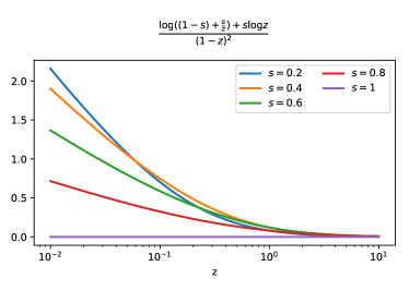
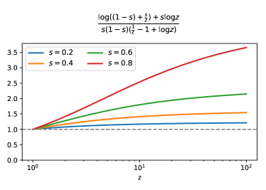
Figure 11: Illustration of Lemma 18 showing that for any $z\geq 1$, $\log\big{(}(1-s)+\tfrac{s}{z}\big{)}+s\log z\geq s(1-s)\big{(}\tfrac{1}{z}-1+\log z\big{)}$.

7.7 Proof of Theorem 4

This proof is very similar to SDCA’s proof [37] but it uses the new convex inequality on the Fenchel conjugate of $\log$ smooth functions from Lemma  16 to get a tighter inequality. We first prove the following lemma which is an equivalent of Lemma 6 from [37] but with convex functions $f_{i}$ that are $L_{i}$-$\log$ smooth instead of being $L_{i}$-gradient Lipschitz.

Lemma 19.

Suppose that we known bounds $\beta_{i}\in-\mathcal{D}_{f^{*}}$ such that $R_{i}=\beta_{i}/\alpha_{i}^{*}\geq 1$ for $i=1,\ldots,n$ and assume that all $f_{i}$ are $L_{i}$-$\log$ smooth with differentiable Fenchel conjugates and that $g$ is 1-strongly convex. Then, if $\alpha^{(t,i)}$ is the value of $\alpha^{(t)}$ when $i$ is sampled at iteration $t$ for Algorithms 1 and 2, we have

$$\sum_{i=1}^{n}s_{i}^{-1}\big{(}D(\alpha^{(t,i)})-D(\alpha^{(t-1)})\big{)}\geq D(\alpha^{*})-D(\alpha^{(t-1)})+G(s_{i},\alpha_{i}^{(t-1)},\alpha_{i}^{*})$$ (26)

for any ${s_{1},\dots,s_{n}}\in[0,1]$, where

$$G(s,\alpha^{(t-1)},\alpha^{*})=\frac{1}{n}\sum_{i=1}^{n}\Big{(}L_{i}\gamma(s_{i},\alpha_{i}^{(t-1)},\alpha_{i}^{*})-\frac{s_{i}}{2\lambda n}\|x_{i}\|^{2}(\alpha_{i}^{*}-\alpha_{i}^{(t-1)})^{2}\Big{)}$$

and

$$\gamma(s_{i},\alpha_{i}^{(t-1)},\alpha_{i}^{*})=\frac{1}{s_{i}}\log\Big{(}1-s_{i}+s_{i}\frac{\alpha_{i}^{*}}{\alpha_{i}^{(t-1)}}\Big{)}-\log\frac{\alpha_{i}^{*}}{\alpha_{i}^{(t-1)}}.$$

Proof.

At iteration $t$, if the dual vector is set to $\alpha^{(t)}$ (and $v^{(t)}=v(\alpha^{(t)})$, see Equation (15)) the dual gain is

$$n(D(\alpha^{(t)})-D(\alpha^{(t-1)}))=\underbrace{\big{(}-f_{i}^{*}(-\alpha_{i}^{t})-\lambda ng^{*}(v^{(t)})\big{)}}_{A_{i}}-\underbrace{\big{(}-f_{i}^{*}(-\alpha_{i}^{(t-1)})-\lambda ng^{*}(v^{(t-1)})\big{)}}_{B_{i}}$$

where $i$ is the index sampled at iteration $t$ (see Line 4). For Algorithm 1, by the definition of $\alpha_{i}^{(t)}$ given on Lines 5 and 6 we have

$$A_{i}=\max_{\begin{subarray}{c}\alpha_{i}\in-\mathcal{D}_{f^{*}}\\ \text{s.t. }\beta_{i}/\alpha_{i}\geq 1\end{subarray}}-f_{i}^{*}(-\alpha_{i})-\lambda ng^{*}\Big{(}\frac{1}{\lambda n}(\alpha_{i}-\alpha_{i}^{(t-1)})x_{i}+\frac{1}{\lambda n}\sum_{j=1}^{n}\alpha_{j}^{(t-1)}x_{j}-\frac{1}{\lambda}\psi\Big{)}.$$

Using the smoothness inequality on $g^{*}$ which is 1-smooth as $g$ is 1-strongly convex,

$$g^{*}(v^{(t-1)}+\Delta v)\leq h(v^{(t-1)},\Delta v)\\ \text{where}\;\;h(v^{(t-1)},\Delta v)=g^{*}(v^{(t-1)})+\nabla g^{*}(v^{(t-1)})^{\top}\Delta v+\frac{1}{2}\|\Delta v\|^{2}.$$

Hence setting $\Delta v$ to $(\lambda n)^{-1}(\alpha_{i}-\alpha_{i}^{(t-1)})x_{i}$ , we can lower bound $A_{i}$ with

$$A_{i}\geq\max_{\begin{subarray}{c}\alpha_{i}\in-\mathcal{D}_{f^{*}}\\ \text{s.t. }\beta_{i}/\alpha_{i}\geq 1\end{subarray}}-f_{i}^{*}(-\alpha_{i})-\lambda nh\big{(}v^{(t-1)},(\lambda n)^{-1}(\alpha_{i}-\alpha_{i}^{(t-1)})x_{i}\big{)}.$$

For Algorithm 2, by definition of $\alpha_{i}^{(t)}$ stated at Lines 5 and 6 combined with the modified argmax relation (16),

$$A_{i}=\max_{\begin{subarray}{c}\alpha_{i}\in-\mathcal{D}_{f^{*}}\\ \text{s.t. }\beta_{i}/\alpha_{i}\geq 1\end{subarray}}-f_{i}^{*}(-\alpha_{i})-\lambda nh\big{(}v^{(t-1)},(\lambda n)^{-1}(\alpha_{i}-\alpha_{i}^{(t-1)})x_{i}\big{)}.$$

As both $\alpha_{i}^{(t-1)}$ and $\alpha_{i}^{*}$ belong to $\{\alpha_{i}\in-\mathcal{D}_{f^{*}},\beta_{i}/\alpha_{i}\geq 1\}$, for any $s_{i}\in[0,1]$, the convex combination $\alpha_{i}=(1-s_{i})\alpha_{i}^{(t-1)}+s_{i}\alpha_{i}^{*}$ belongs to it as well. Hence, for both algorithms, $A_{i}$ is higher than the previous quantity evaluated at this specific $\alpha_{i}$. Namely,

$$A_{i}\geq-f_{i}^{*}\big{(}-\big{(}(1-s_{i})\alpha_{i}^{(t-1)}+s_{i}\alpha_{i}^{*}\big{)}\big{)}-\lambda nh\big{(}v^{(t-1)},(\lambda n)^{-1}s_{i}(\alpha_{i}^{*}-\alpha_{i}^{(t-1)})x_{i}\big{)}.$$

We then use Lemma 16, in which $-\alpha_{i}^{*}\in\mathcal{D}_{f^{*}}$ stands for $x$ and $-\alpha_{i}^{(t-1)}\in\mathcal{D}_{f^{*}}$ for $y$:

$$(1-s_{i})f_{i}^{*}(-\alpha_{i}^{(t-1)})+s_{i}f_{i}^{*}(-\alpha_{i}^{*})-f_{i}^{*}(-(1-s_{i})\alpha_{i}^{(t-1)}-s_{i}\alpha_{i}^{*})\geq s_{i}L_{i}\gamma(s_{i},\alpha_{i}^{(t-1)},\alpha_{i}^{*})$$

where

$$\gamma(s_{i},\alpha_{i}^{(t-1)},\alpha_{i}^{*})=\frac{1}{s_{i}}\log\Big{(}1-s_{i}+s_{i}\frac{\alpha_{i}^{*}}{\alpha_{i}^{(t-1)}}\Big{)}-\log\frac{\alpha_{i}^{*}}{\alpha_{i}^{(t-1)}}.$$

This inequality is used instead of the strong convex inequality of the classic SDCA analysis [37]. If we plug this inequality into $A_{i}$ we obtain

$$A_{i} \geq-s_{i}f^{*}(-\alpha_{i}^{*})-(1-s_{i})f^{*}(-\alpha_{i}^{(t-1)})+s_{i}L_{i}\gamma(s_{i},\alpha_{i}^{(t-1)},\alpha_{i}^{*})$$

$$\quad\quad-\lambda ng^{*}(v^{(t-1)})-s_{i}(\alpha_{i}^{*}-\alpha_{i}^{(t-1)})x_{i}^{\top}\nabla g^{*}(v^{(t-1)})-\frac{s_{i}^{2}(\alpha_{i}^{*}-\alpha_{i}^{(t-1)})^{2}}{2\lambda n}\|x_{i}\|^{2}$$

$$=-s_{i}(f^{*}(-\alpha_{i}^{*})-f^{*}(-\alpha_{i}^{(t-1)}))-f^{*}(-\alpha_{i}^{(t-1)})-\lambda ng^{*}(v^{(t-1)})$$

$$\quad\quad-s_{i}(\alpha_{i}^{*}-\alpha_{i}^{(t-1)})x_{i}^{\top}\nabla g^{*}(v^{(t-1)})+s_{i}\Big{(}L_{i}\gamma(s_{i},\alpha_{i}^{(t-1)},\alpha_{i}^{*})-\frac{s_{i}}{2\lambda n}\|x_{i}\|^{2}(\alpha_{i}^{*}-\alpha_{i}^{(t-1)})^{2}\Big{)}.$$

Hence, we retrieve $B_{i}$ and rewrite the previous inequality as

$$s_{i}^{-1}(A_{i}-B_{i}) \geq-\big{(}f^{*}(-\alpha_{i}^{*})-f^{*}(-\alpha_{i}^{(t-1)})\big{)}-(\alpha_{i}^{*}-\alpha_{i}^{(t-1)})x_{i}^{\top}\nabla g^{*}(v^{(t-1)})$$

$$\quad\quad+L_{i}\gamma(s_{i},\alpha_{i}^{(t-1)},\alpha_{i}^{*})-\frac{s_{i}}{2\lambda n}\|x_{i}\|^{2}(\alpha_{i}^{*}-\alpha_{i}^{(t-1)})^{2}.$$

We can sum over all possible sampled $i$ and weight each entry with $s_{i}^{-1}$ to obtain

$$\sum_{i=1}^{n}s_{i}^{-1}(A_{i}-B_{i}) \geq-\sum_{i=1}^{n}\Big{(}f^{*}(-\alpha_{i}^{*})-f^{*}(-\alpha_{i}^{(t-1)})\Big{)}-\bigg{\langle}\nabla g^{*}(v^{(t-1)})\;\Big{|}~\;\sum_{i=1}^{n}(\alpha_{i}^{*}-\alpha_{i}^{(t-1)})x_{i}\bigg{\rangle}$$

$$\quad\quad+\sum_{i=1}^{n}\Big{(}L_{i}\gamma(s_{i},\alpha_{i}^{(t-1)},\alpha_{i}^{*})-\frac{s_{i}}{2\lambda n}\|x_{i}\|^{2}(\alpha_{i}^{*}-\alpha_{i}^{(t-1)})^{2}\Big{)}.$$ (27)

Then since $g^{*}$ is convex, we obtain

$$\bigg{\langle}\nabla g^{*}(v^{(t-1)})\;\Big{|}~\;\sum_{i=1}^{n}(\alpha_{i}^{*}-\alpha_{i}^{(t-1)})x_{i}\bigg{\rangle} =\big{\langle}\nabla g^{*}(v^{(t-1)})\;|\;\lambda n(v(\alpha^{*})-v^{(t-1)})\big{\rangle}$$

$$\leq\lambda n\big{(}g^{*}(v(\alpha^{*}))-g^{*}(v^{(t-1)})\big{)},$$

which can be injected in Equation (7.7) leading to

$$\sum_{i=1}^{n}s_{i}^{-1}(A_{i}-B_{i}) \geq-\sum_{i=1}^{n}\Big{(}f^{*}(-\alpha_{i}^{*})-f^{*}(-\alpha_{i}^{(t-1)})\Big{)}+\lambda ng^{*}(v(\alpha^{*}))-\lambda ng^{*}(v^{(t-1)})$$

$$\quad\quad+\sum_{i=1}^{n}\Big{(}L_{i}\gamma(s_{i},\alpha_{i}^{(t-1)},\alpha_{i}^{*})-\frac{s_{i}}{2\lambda n}\|x_{i}\|^{2}(\alpha_{i}^{*}-\alpha_{i}^{(t-1)})^{2}\Big{)}.$$

Finally, since $A_{i}-B_{i}=n(D(\alpha^{(t,i)})-D(\alpha^{(t-1)}))$, we obtain

$$\sum_{i=1}^{n}s_{i}^{-1}\big{(}D(\alpha^{(t,i)})-D(\alpha^{(t-1)})\big{)}\\ \geq D(\alpha^{*})-D(\alpha^{(t-1)})+\frac{1}{n}\sum_{i=1}^{n}\Big{(}L_{i}\gamma(s_{i},\alpha_{i}^{(t-1)},\alpha_{i}^{*})-\frac{s_{i}}{2\lambda n}\|x_{i}\|^{2}(\alpha_{i}^{*}-\alpha_{i}^{(t-1)})^{2}\Big{)}.$$

This concludes the proof of Lemma 19. ∎

From Lemma 19, we obtain a contraction speed as soon as $G(s,\alpha^{(t-1)},\alpha^{*})\geq 0$. If $\alpha_{i}^{(t-1)}\neq\alpha_{i}^{*}$ this is obtained if

$$\forall i\in\{1,\dots,n\},\quad L_{i}\gamma(s_{i},\alpha_{i}^{(t-1)},\alpha_{i}^{*})-\frac{s_{i}}{2\lambda n}\|x_{i}\|^{2}(\alpha_{i}^{*}-\alpha_{i}^{(t-1)})^{2}\geq 0$$ (28)

$$\Leftrightarrow\quad\forall i\in\{1,\dots,n\},\quad\frac{\gamma(s_{i},\alpha_{i}^{(t-1)},\alpha_{i}^{*})}{\Big{(}1-\frac{\alpha_{i}^{(t-1)}}{\alpha_{i}^{*}}\Big{)}^{2}}-s_{i}\frac{\|x_{i}\|^{2}{\alpha_{i}^{*}}^{2}}{2\lambda nL_{i}}\geq 0.$$

By definition of $\gamma$ we have

$$\frac{\gamma(s_{i},\alpha_{i}^{(t-1)},\alpha_{i}^{*})}{\Big{(}1-\frac{\alpha_{i}^{(t-1)}}{\alpha_{i}^{*}}\Big{)}^{2}}=\frac{\log\Big{(}1-s_{i}+s_{i}\frac{\alpha_{i}^{*}}{\alpha_{i}^{(t-1)}}\Big{)}-s_{i}\log\frac{\alpha_{i}^{*}}{\alpha_{i}^{(t-1)}}}{s_{i}\Big{(}1-\frac{\alpha_{i}^{(t-1)}}{\alpha_{i}^{*}}\Big{)}^{2}}.$$

As $\alpha_{i}^{(t-1)}/\alpha_{i}^{*}$ is bounded by $\beta_{i}/\alpha_{i}^{*}$, we apply Lemma 17 to obtain

$$\frac{\gamma(s_{i},\alpha_{i}^{(t-1)},\alpha_{i}^{*})}{\Big{(}1-\frac{\alpha_{i}^{(t-1)}}{\alpha_{i}^{*}}\Big{)}^{2}}\geq\frac{\log\Big{(}1-s_{i}+s_{i}\frac{\alpha_{i}^{*}}{\beta_{i}}\Big{)}-s_{i}\log\frac{\alpha_{i}^{*}}{\beta_{i}}}{s_{i}\Big{(}1-\frac{\beta_{i}}{\alpha_{i}^{*}}\Big{)}^{2}},$$

and as $\beta_{i}/\alpha_{i}^{*}\geq 1$, we can apply Lemma 18 leading to

$$\frac{\gamma(s_{i},\alpha_{i}^{(t-1)},\alpha_{i}^{*})}{\Big{(}1-\frac{\alpha_{i}^{(t-1)}}{\alpha_{i}^{*}}\Big{)}^{2}}\geq\frac{\big{(}1-s_{i}\big{)}\Big{(}\frac{\alpha_{i}^{*}}{\beta_{i}}-1+\log\frac{\beta_{i}}{\alpha_{i}^{*}}\Big{)}}{\Big{(}1-\frac{\beta_{i}}{\alpha_{i}^{*}}\Big{)}^{2}}.$$

Finally the convergence condition from Equation (28) is satisfied when

$$\forall i\in\{1,\dots,n\},\quad\big{(}1-s_{i}\big{)}\bigg{(}\frac{\alpha_{i}^{*}}{\beta_{i}}-1+\log\frac{\beta_{i}}{\alpha_{i}^{*}}\bigg{)}-s_{i}\frac{\|x_{i}\|^{2}{\alpha_{i}^{*}}^{2}}{2\lambda nL_{i}}\bigg{(}1-\frac{\beta_{i}}{\alpha_{i}^{*}}\bigg{)}^{2}\geq 0$$

which is true for any $s_{i}\in[0,\sigma_{i}]$ where

$$\sigma_{i}=\left(1+\frac{\|x_{i}\|^{2}{\alpha_{i}^{*}}^{2}}{2\lambda nL_{i}}\frac{\Big{(}1-\frac{\beta_{i}}{\alpha_{i}^{*}}\Big{)}^{2}}{\frac{\alpha_{i}^{*}}{\beta_{i}}+\log\frac{\beta_{i}}{\alpha_{i}^{*}}-1}\right)^{-1}.$$

Theorem 4 is obtained by sampling uniformly $i$, meaning haing all $s_{i}$ equal. Hence, to fulfill Equation (28), we set

$$s_{i}=\min_{j\in\{1,\dots,n\}}\sigma_{j}$$ (29)

for all $i\in\{1,\dots,n\}$. We then lower bound the expectation of $D(\alpha^{(t)})-D(\alpha^{(t-1)})$ over all possible sampled $i$ and obtain

$$\mathbb{E}[D(\alpha^{(t)})-D(\alpha^{(t-1)})]=\frac{1}{n}\sum_{i=1}^{n}D(\alpha^{(t,i)})-D(\alpha^{(t-1)})\geq\frac{\min_{j}\sigma_{j}}{n}(D(\alpha^{*})-D(\alpha^{(t-1)})),$$

by multiplying Equation (26) with $\min_{j\in\{1,\dots,n\}}\sigma_{j}/n$ and removing the quantity $G^{(t-1)}\geq 0$. This leads to the following convergence speed after $t$ iterations,

$$\mathbb{E}[D(\alpha^{*})-D(\alpha^{(t)})]\leq\Big{(}1-\frac{\min_{j}\sigma_{j}}{n}\Big{)}^{t}(D(\alpha^{*})-D(\alpha^{(0)})),$$

which concludes the proof of Theorem 4. $\hfill\qed$

7.8 Proof of Theorem 5

Instead of taking all $s_{i}$ equal as in the uniform sampling setting (see Equation (29)), we rather parametrize $s_{i}$ by $\frac{\bar{\sigma}}{\rho_{i}n}$ where $\rho_{i}$ is the probability of sampling $i$. Then, we obtain the following expectation under $\rho$,

$$\mathbb{E}_{\rho}[D(\alpha^{(t)})-D(\alpha^{(t-1)})]=\sum_{i=1}^{n}\rho_{i}D(\alpha^{(t,i)})-D(\alpha^{(t-1)}).$$

Since we have $\rho_{i}=\frac{n}{\bar{\sigma}}s_{i}^{-1}$ we obtain the following inequality using Lemma 19:

$$\mathbb{E}_{\rho}[D(\alpha^{(t)})-D(\alpha^{(t-1)})]\geq\frac{\bar{\sigma}}{n}\Big{(}D(\alpha^{*})-D(\alpha^{(t-1)})+G\big{(}\bar{\sigma}(\rho n)^{-1},\alpha^{(t-1)},\alpha^{*}\big{)}\Big{)}.$$ (30)

To ensure that $G\big{(}\bar{\sigma}(\rho n)^{-1},\alpha^{(t-1)},\alpha^{*}\big{)}\geq 0$ while keeping the biggest gain, we must satisfy the constraint from Equation (28) and find feasible $\rho$ and $\bar{\sigma}$ that maximize the following problem:

$$\max_{\bar{\sigma}}\bar{\sigma}\quad\text{subject to}\quad\frac{\bar{\sigma}}{\rho_{i}n}\in[0,\sigma_{i}],\quad\rho_{i}\geq 0,\quad\sum_{i=1}^{n}\rho_{i}=1.$$

This problem is solved by Proposition 1 of [42] and leads to the following choices:

$$\rho_{i}=\frac{\sigma_{i}^{-1}}{\sum_{j=1}^{n}\sigma_{j}^{-1}}\quad\text{and}\quad\bar{\sigma}=\Big{(}\frac{1}{n}\sum_{i=1}^{n}\sigma_{i}^{-1}\Big{)}^{-1}.$$ (31)

This choice for $\rho$ and $\bar{\sigma}$ ensures $G(\bar{\sigma}(\rho n)^{-1},\alpha^{(t-1)},\alpha^{*})\geq 0$ hence Equation (30) without $G\big{(}\bar{\sigma}(\rho n)^{-1},\alpha^{(t-1)},\alpha^{*}\big{)}$ leads to

$$\mathbb{E}_{\rho}[D(\alpha^{(t)})-D(\alpha^{(t-1)})]\geq\frac{\bar{\sigma}}{n}(D(\alpha^{*})-D(\alpha^{(t-1)})),$$

and finally, after $t$ iterations, we have

$$\mathbb{E}[D(\alpha^{*})-D(\alpha^{(t)})]\leq\Big{(}1-\frac{\bar{\sigma}}{n}\Big{)}^{t}(D(\alpha^{*})-D(\alpha^{(0)})),$$

which concludes the proof of Theorem 5. $\hfill\qed$

7.9 Proof of Proposition 6

With $f_{i}^{*}(-\alpha_{i})=-y_{i}-y_{i}\log\frac{\alpha_{i}}{y_{i}}$, let

$$\phi(\alpha_{i})=y_{i}+y_{i}\log\frac{\alpha_{i}}{y_{i}}-\frac{\lambda n}{2}\Big{\|}w^{(t-1)}+(\lambda n)^{-1}(\alpha_{i}-\alpha_{i}^{(t-1)})x_{i}\Big{\|}^{2}$$

be the function to optimize. Note that $\phi$ is a concave function from $-\mathcal{D}_{f^{*}}$ to $\mathbb{R}$ and hence it reaches its minimum if its gradient is zero:

$$\phi^{\prime}(\alpha_{i})=\frac{y_{i}}{\alpha_{i}}-x_{i}^{\top}w^{(t-1)}-\frac{\|x_{i}\|^{2}}{\lambda n}(\alpha_{i}-\alpha_{i}^{(t-1)})=0.$$

This second order equation in $\alpha_{i}$ has a unique positive solution, the one stated in Proposition 6.

7.10 Proof of Proposition 7

Given that we are using Ridge regularization, the values of $f_{i}^{*}$ and $g^{*}$ are

$$f_{i}^{*}(v)=-y_{i}-y_{i}\log\Big{(}\frac{-v}{y_{i}}\Big{)}\quad\text{and}\quad g^{*}(w)=g(w)=\frac{1}{2}\|w\|^{2}.$$

Hence the conditions at optimum (5) and (14) become

$$w^{*}=\frac{1}{\lambda n}\sum_{i=1}^{n}\alpha_{i}^{*}x_{i}-\frac{1}{\lambda}\psi\quad\text{and}\quad\forall i\in\{1,\dots n\},\quad\alpha_{i}^{*}=\frac{y_{i}}{{w^{*}}^{\top}x_{i}}.$$ (32)

By combining both equations with Equation (32), we have

$$\forall i\in\{1,\dots n\},\quad\alpha_{i}^{*}=\frac{\lambda ny_{i}}{\sum_{j=1}^{n}\alpha_{j}^{*}x_{j}^{\top}x_{i}-n\psi^{\top}x_{i}}.$$ (33)

Since the inner products $x_{i}^{\top}x_{j}$ and $\alpha_{i}$ are non-negative, we can remove the terms $\sum_{j\neq i}\alpha_{j}^{*}x_{j}^{\top}x_{i}$ and upper bound the dual variable with

$$\forall i\in\{1,\dots n\},\quad\alpha_{i}^{*}\leq\frac{\lambda ny_{i}}{\alpha_{i}^{*}\|x_{i}\|^{2}-n\psi^{\top}x_{i}}.$$

By solving this second order inequality, we can derive the following upper bound for all $\alpha_{i}^{*}$:

$$\alpha_{i}^{*}\leq\frac{1}{2\|x_{i}\|^{2}}\Big{(}n\psi^{\top}x_{i}+\sqrt{(n\psi^{\top}x_{i})^{2}+4\lambda ny_{i}\|x_{i}\|^{2}}\Big{)},$$

which concludes the proof. $\hfill\qed$

7.11 Proof of Remark 2

At each iteration the closed form solution is given by Proposition 6:

$$\alpha^{t}_{i}=\frac{1}{2}\Bigg{(}\sqrt{\Big{(}\alpha_{i}^{(t-1)}-\frac{\lambda n}{\|x_{i}\|^{2}}x_{i}^{\top}w^{(t-1)}\Big{)}^{2}+4\lambda n\frac{y_{i}}{\|x_{i}\|^{2}}}+\alpha_{i}^{(t-1)}-\frac{\lambda n}{\|x_{i}\|^{2}}x_{i}^{\top}w^{(t-1)}\Bigg{)}.$$

Since the inner products $x_{i}^{\top}x_{j}$ are non-negative, we obtain

$$\alpha_{i}^{(t-1)}-\frac{\lambda n}{\|x_{i}\|^{2}}x_{i}^{\top}w^{(t-1)}=n\frac{\psi^{\top}x_{i}}{\|x_{i}\|^{2}}-\sum_{j\neq i}\alpha_{j}^{(t-1)}\frac{x_{j}^{\top}x_{i}}{\|x_{i}\|^{2}}\leq n\frac{\psi^{\top}x_{i}}{\|x_{i}\|^{2}}$$

and since $\alpha^{t}_{i}$ is increasing with ${(\alpha_{i}^{(t-1)}-\frac{\lambda n}{\|x_{i}\|^{2}}x_{i}^{\top}w^{(t-1)})}$, we obtain

$$\alpha^{t}_{i}\leq\frac{1}{2}\Bigg{(}\sqrt{n\frac{\psi^{\top}x_{i}^{2}}{\|x_{i}\|^{4}}+4\lambda n\frac{y_{i}}{\|x_{i}\|^{2}}}+n\frac{\psi^{\top}x_{i}}{\|x_{i}\|^{2}}\Bigg{)}=\beta_{i},$$

which concludes the proof. $\hfill\qed$

7.12 Proof of Proposition 8

This proposition easily follows from the following computation

$$\zeta^{*} =\operatorname*{arg\,max}_{\zeta\in(0,+\infty)^{n}}\frac{1}{n}\sum_{i=1}^{n}-y_{i}-y_{i}\log\frac{\zeta_{i}}{y_{i}}-\lambda g^{*}\bigg{(}\frac{1}{\lambda n}\sum_{i=1}^{n}\zeta_{i}\xi_{i}-\frac{1}{\lambda}\psi\bigg{)}$$

$$=\operatorname*{arg\,max}_{\zeta\in(0,+\infty)^{n}}\frac{1}{n}\sum_{i=1}^{n}-y_{i}-y_{i}\log\frac{\zeta_{i}}{y_{i}}+y_{i}\log(c_{i})-\lambda g^{*}\bigg{(}\frac{1}{\lambda n}\sum_{i=1}^{n}c_{i}\zeta_{i}x_{i}-\frac{1}{\lambda}\psi\bigg{)}$$

$$=\operatorname*{arg\,max}_{\zeta\in(0,+\infty)^{n}}D(c\cdot\zeta),$$

where $D$ is the original dual problem and $c\cdot\zeta$ is the element wise product of the vectors $c$ and $\zeta$. Then, since

$$\operatorname*{arg\,max}_{x}\{x\mapsto f(cx)\}=\frac{1}{c}\operatorname*{arg\,max}\{x\mapsto f(x)\},$$

which remains valid in the multivariate case, we obtain $\zeta^{*}_{i}=\alpha_{i}^{*}/c_{i}$ for any $i=1,\dots,n$. $\hfill\qed$

7.13 Proof of Proposition 9

Using $\alpha^{*}=\bar{\alpha}\kappa$ the dual problem becomes one dimensional

$$D(\bar{\alpha})=\frac{1}{n}\sum_{i=1}^{n}y_{i}+y_{i}\log\tfrac{\kappa_{i}\bar{\alpha}}{y_{i}}-\frac{\lambda}{2}\bigg{\|}\frac{1}{\lambda n}\sum_{i=1}^{n}\kappa_{i}\bar{\alpha}x_{i}-\frac{1}{\lambda}\psi\bigg{\|}^{2}.$$

This problem is concave in $\bar{\alpha}$ and the optimal $\bar{\alpha}$ is obtained by setting the derivative to zero:

$$D^{\prime}(\bar{\alpha})=\frac{1}{n}\sum_{i=1}^{n}\frac{y_{i}}{\bar{\alpha}}-\bigg{\langle}\frac{1}{\lambda n}\bar{\alpha}\sum_{i=1}^{n}\kappa_{i}x_{i}-\frac{1}{\lambda}\psi\;\Big{|}\;\frac{1}{n}\sum_{i=1}^{n}\kappa_{i}x_{i}\bigg{\rangle}=0.$$

This leads to the following second order equation

$$\bigg{\|}\frac{1}{n}\sum_{i=1}^{n}\kappa_{i}x_{i}\bigg{\|}^{2}\bar{\alpha}^{2}-\bigg{\langle}\psi\;\Big{|}\;\frac{1}{n}\sum_{i=1}^{n}\kappa_{i}x_{i}\bigg{\rangle}\bar{\alpha}-\frac{\lambda}{n}\sum_{i=1}^{n}y_{i}=0,$$

which has a unique positive solution

$$\bar{\alpha}=\frac{1}{2\big{\|}\frac{1}{n}\sum_{i=1}^{n}\kappa_{i}x_{i}\big{\|}^{2}}\left(\bigg{\langle}\psi\;\Big{|}\;\frac{1}{n}\sum_{i=1}^{n}\kappa_{i}x_{i}\bigg{\rangle}+\sqrt{\bigg{\langle}\psi\;\Big{|}\;\frac{1}{n}\sum_{i=1}^{n}\kappa_{i}x_{i}\bigg{\rangle}^{2}+4\frac{\lambda}{n}\sum_{i=1}^{n}y_{i}\bigg{\|}\frac{1}{n}\sum_{i=1}^{n}\kappa_{i}x_{i}\bigg{\|}^{2}}\right),$$

and concludes the proof. $\hfill\qed$

References

- [1] F. Bach et al. Self-concordant analysis for logistic regression. Electronic Journal of Statistics, 4:384–414, 2010.
- [2] E. Bacry, T. Jaisson, and J.-F. Muzy. Estimation of slowly decreasing hawkes kernels: application to high-frequency order book dynamics. Quantitative Finance, 16(8):1179–1201, 2016.
- [3] E. Bacry, I. Mastromatteo, and J.-F. Muzy. Hawkes processes in finance. Market Microstructure and Liquidity, 1(01):1550005, 2015.
- [4] H. H. Bauschke, J. Bolte, and M. Teboulle. A descent lemma beyond lipschitz gradient continuity: first-order methods revisited and applications. Mathematics of Operations Research, 42(2):330–348, 2016.
- [5] A. Beck and M. Teboulle. A fast iterative shrinkage-thresholding algorithm for linear inverse problems. SIAM journal on imaging sciences, 2(1):183–202, 2009.
- [6] M. Bertero, P. Boccacci, G. Desiderà, and G. Vicidomini. Image deblurring with poisson data: from cells to galaxies. Inverse Problems, 25(12):123006, 2009.
- [7] D. P. Bertsekas. Nonlinear programming. Athena scientific Belmont, 1999.
- [8] H. C. Boshuizen and E. J. Feskens. Fitting additive poisson models. Epidemiologic Perspectives & Innovations, 7(1):4, 2010.
- [9] Y. Chen, D. Pavlov, and J. F. Canny. Large-scale behavioral targeting. In Proceedings of the 15th ACM SIGKDD international conference on Knowledge discovery and data mining, pages 209–218. ACM, 2009.
- [10] P. Cortez, A. Cerdeira, F. Almeida, T. Matos, and J. Reis. Modeling wine preferences by data mining from physicochemical properties. Decision Support Systems, 47(4):547–553, 2009.
- [11] D. J. Daley and D. Vere-Jones. An introduction to the theory of point processes: volume II: general theory and structure. Springer Science & Business Media, 2007.
- [12] A. De, I. Valera, N. Ganguly, S. Bhattacharya, and M. G. Rodriguez. Learning and forecasting opinion dynamics in social networks. In Advances in Neural Information Processing Systems, pages 397–405, 2016.
- [13] A. Defazio, F. Bach, and S. Lacoste-Julien. Saga: A fast incremental gradient method with support for non-strongly convex composite objectives. In Advances in neural information processing systems, pages 1646–1654, 2014.
- [14] M. Farajtabar, Y. Wang, M. G. Rodriguez, S. Li, H. Zha, and L. Song. Coevolve: A joint point process model for information diffusion and network co-evolution. In Advances in Neural Information Processing Systems, pages 1954–1962, 2015.
- [15] K. Fernandes, P. Vinagre, and P. Cortez. A proactive intelligent decision support system for predicting the popularity of online news. In Portuguese Conference on Artificial Intelligence, pages 535–546. Springer, 2015.
- [16] Z. T. Harmany, R. F. Marcia, and R. M. Willett. This is spiral-tap: Sparse poisson intensity reconstruction algorithms—theory and practice. IEEE Transactions on Image Processing, 21(3):1084–1096, 2012.
- [17] A. G. Hawkes and D. Oakes. A cluster process representation of a self-exciting process. Journal of Applied Probability, 11(3):493–503, 1974.
- [18] E. Hazan and H. Luo. Variance-reduced and projection-free stochastic optimization. In International Conference on Machine Learning, pages 1263–1271, 2016.
- [19] R. Johnson and T. Zhang. Accelerating stochastic gradient descent using predictive variance reduction. In Advances in Neural Information Processing Systems, pages 315–323, 2013.
- [20] M. Lichman. UCI machine learning repository, 2013.
- [21] H. Lu, R. M. Freund, and Y. Nesterov. Relatively smooth convex optimization by first-order methods, and applications. SIAM Journal on Optimization, 28(1):333–354, 2018.
- [22] M. Lukasik, P. Srijith, D. Vu, K. Bontcheva, A. Zubiaga, and T. Cohn. Hawkes processes for continuous time sequence classification: an application to rumour stance classification in twitter. In Proceedings of 54th Annual Meeting of the Association for Computational Linguistics, pages 393–398. Association for Computational Linguistics, 2016.
- [23] G. Mohler et al. Modeling and estimation of multi-source clustering in crime and security data. The Annals of Applied Statistics, 7(3):1525–1539, 2013.
- [24] S. Moro, P. Rita, and J. Coelho. Stripping customers’ feedback on hotels through data mining: the case of las vegas strip. Tourism Management Perspectives, 23:41–52, 2017.
- [25] S. Moro, P. Rita, and B. Vala. Predicting social media performance metrics and evaluation of the impact on brand building: A data mining approach. Journal of Business Research, 69(9):3341–3351, 2016.
- [26] Y. Nesterov. Introductory lectures on convex optimization: A basic course, volume 87. Springer Science & Business Media, 2013.
- [27] Y. Nesterov and A. Nemirovskii. Interior-point polynomial algorithms in convex programming. SIAM, 1994.
- [28] J. Nocedal. Updating quasi-newton matrices with limited storage. Mathematics of computation, 35(151):773–782, 1980.
- [29] J. Nocedal and S. J. Wright. Nonlinear Equations. Springer, 2006.
- [30] Y. Ogata. Seismicity analysis through point-process modeling: A review. Pure & Applied Geophysics, 155(2-4):471, 1999.
- [31] R. L. Priol, A. Touati, and S. Lacoste-Julien. Adaptive stochastic dual coordinate ascent for conditional random fields. (291), 2018.
- [32] Z. Qu, P. Richtárik, M. Takác, and O. Fercoq. Sdna: Stochastic dual newton ascent for empirical risk minimization. In International Conference on Machine Learning, pages 1823–1832, 2016.
- [33] M. Rambaldi, E. Bacry, and F. Lillo. The role of volume in order book dynamics: a multivariate hawkes process analysis. Quantitative Finance, 17(7):999–1020, 2017.
- [34] H. Robbins and S. Monro. A stochastic approximation method. The annals of mathematical statistics, pages 400–407, 1951.
- [35] M. Schmidt, N. L. Roux, and F. Bach. Minimizing finite sums with the stochastic average gradient. arXiv preprint arXiv:1309.2388, 2013.
- [36] S. Shalev-Shwartz and T. Zhang. Stochastic dual coordinate ascent methods for regularized loss minimization. Journal of Machine Learning Research, 14(Feb):567–599, 2013.
- [37] S. Shalev-Shwartz and T. Zhang. Accelerated proximal stochastic dual coordinate ascent for regularized loss minimization. In International Conference on Machine Learning, pages 64–72, 2014.
- [38] T. Sun and Q. Tran-Dinh. Generalized self-concordant functions: a recipe for newton-type methods. Mathematical Programming, pages 1–69, 2017.
- [39] C. Tan, S. Ma, Y.-H. Dai, and Y. Qian. Barzilai-borwein step size for stochastic gradient descent. In Advances in Neural Information Processing Systems, pages 685–693, 2016.
- [40] Q. Tran-Dinh, A. Kyrillidis, and V. Cevher. Composite self-concordant minimization. The Journal of Machine Learning Research, 16(1):371–416, 2015.
- [41] L. Xiao and T. Zhang. A proximal stochastic gradient method with progressive variance reduction. SIAM Journal on Optimization, 24(4):2057–2075, 2014.
- [42] P. Zhao and T. Zhang. Stochastic optimization with importance sampling for regularized loss minimization. In Proceedings of the 32nd International Conference on Machine Learning (ICML-15), pages 1–9, 2015.