A finite element method for the Monge–Ampère equation with optimal transport boundary conditions

Abstract.

We address the numerical solution via Galerkin type methods of the Monge–Ampère equation with optimal transport boundary conditions, arising in optimal mass transport, geometric optics and mesh/grid movement techniques. This fully nonlinear elliptic problem admits a linearisation via a Newton–Raphson iteration, which leads to a sequence of elliptic equations in nondivergence form, with oblique derivative boundary conditions. We discretise these by employing the nonvariational finite element method, which leads to empirically observed optimal convergence rates, provided recovery techinques are used to approximate the gradient and the Hessian of the unknown functions. We provide extensive numerical testing to illustrate the strengths of our approach and the potential applications in optics and mesh movement.

1. Introduction

1.1. The Monge–Ampère problem

Given $d\geq 1$, two convex domains (i.e., open and bounded subsets) of $\mathbb{R}^{d}$, $\varOmega$ and $\varUpsilon$, and two uniformly positive functions $\rho:\varOmega\to\mathbb{R}$ and $\sigma:\varUpsilon\to\mathbb{R}$ (thought as mass densities) with equal total mass ($\smallint_{\varOmega}{\rho}=\smallint_{\varUpsilon}{\sigma}$), the Monge–Ampère problem for optimal transport (MAOT) consists of finding a function $u:\varOmega\to\mathbb{R}$ satisfying the following domain transport condition

$$\nabla u(\varOmega)=\varUpsilon,$$ (1)

and the partial differential equation (PDE)

$$\det\operatorname{D}\!^{2}u(\boldsymbol{x})=\frac{\rho(\boldsymbol{x})}{\sigma(\nabla u(\boldsymbol{x}))}\text{ for }\boldsymbol{x}\in\varOmega,$$ (2)

where $\nabla u(\boldsymbol{x})$ and $\operatorname{D}\!^{2}u(\boldsymbol{x})$ respectively denote the gradient vector and Hessian tensor (or matrix) of $u$ at $\boldsymbol{x}$.

The PDE (2) is commonly known as the Monge–Ampère equation and the domain transport condition in (1) is called the transport boundary condition (also known as second boundary condition) because with (2) it defines a boundary value problem associated to the optimal transport problem of finding a map $\boldsymbol{t}:\varOmega\to\mathbb{R}^{d}$, known as the transport map or transport field, such that

$$\boldsymbol{t}(\varOmega)=\varUpsilon\text{ and }\sigma(\boldsymbol{t}(\boldsymbol{x}))\det\operatorname{D}\!\boldsymbol{t}(\boldsymbol{x})=\rho(\boldsymbol{x}).$$ (3)

Here the equation can be interpreted as the change of variables $\boldsymbol{y}=\boldsymbol{t}(\boldsymbol{x})$, which clarifies why we required equality of mass for $\rho$ and $\sigma$ as

$$\operatorname{d}\!\boldsymbol{y}=\det\operatorname{D}\!\boldsymbol{t}(\boldsymbol{x})\operatorname{d}\!\boldsymbol{x}$$ (4)

and thus

$$\int_{\varOmega}\rho(\boldsymbol{x})\operatorname{d}\!\boldsymbol{x}=\int_{\varUpsilon}\sigma(\boldsymbol{t}(\boldsymbol{x}))\det\operatorname{D}\!\boldsymbol{t}(\boldsymbol{x})\operatorname{d}\!\boldsymbol{x}=\int_{\varUpsilon}\sigma(\boldsymbol{y})\operatorname{d}\!\boldsymbol{y}.$$ (5)

At first sight it may appear that (1) is not a boundary condition, since values of the gradient are prescribed in the interior of $\varOmega$ instead of its boundary, $\partial\varOmega$. But on closer inspection, and as shown in Urbas (1997), this condition, thanks to the convexity of the domains $\varOmega$ and $\varUpsilon$, is in fact equivalent to the boundary-only condition

$$\boldsymbol{t}(\partial\varOmega)=\partial\varUpsilon.$$ (6)

Thanks to the polar factorization of transport maps discovered by Brenier (1991), a field $\boldsymbol{t}$, with simply connected uniformly convex domains $\varOmega$ and $\varUpsilon$, satisfying (3), exists if and only if there exists a uniformly convex function $u:\varOmega\to\mathbb{R}$, such that $\boldsymbol{t}=\nabla u$, satisfying (2) and (1); and the latter can be replaced by

$$\nabla u(\partial\varOmega)=\partial\varUpsilon.$$ (7)

In Prins et al. (2014) the equivalence is proved under the weaker assumption that $\varOmega$ and $\varUpsilon$ are simply connected domains, the existence and uniqueness results proven by Urbas (1997) require that both $\varOmega$ and $\varUpsilon$ are uniformly convex. As such this will be our general assumption unless stated otherwise. An overview can also be found in Prins et al. (2014) and more in Villani (2003, Ch.4).

For $1=d$ the Monge–Ampère equation reduces to the textbook (linear) Poisson equation and the transport boundary condition to a nonlinear Neumann boundary condition. For $2\leq d$, equation (2) is a fully nonlinear elliptic equation, while the boundary condition (1) equation can be interpreted as a nonlinear condition on the gradient (or a Hamilton–Jacobi equation) of the function $\nabla u$.

MAOT arises in many areas of mathematics, such as differential geometry, meteorology, and the design of free form reflectors. One particular meteorological application of the MAOT problem is the incorporation of moving meshes in the solution of meteorological partial differential equations. Budd et al. (2013) successfully coupled a parabolic MAOT method for the construction of a moving mesh in two-dimensions to a pressure correction method. In this case the MAOT problem serves to generate a moving mesh on which the PDE is solved numerically (Budd et al., 2015).

The linearisation of MA type equations typically results in a sequence of nondivergence form elliptic equations. Such problems do not, in general, possess a weak formulation, and as such, standard conforming finite element methods must be either restricted (Nochetto and Zhang, 2018), modified into mixed forms (Lakkis and Pryer, 2011; Gallistl, 2017a), nonconforming (discontinuous Galerkin) (Smears and Süli, 2013; Kawecki, 2017b), or obtained in the limit of fourth-order perturbations (Feng and Neilan, 2014). Lakkis and Pryer (2013, 2011) proposed a continuous Galerkin finite element method, called the nonvariational finite element method (NVFEM), which approximates solutions of nondivergence form elliptic problems, with Dirichlet boundary conditions. Other notable discontinuous Galerkin finite element methods were derived by Smears and Süli (2013) in the context of convex polytopal domains, as well as Kawecki (2017a) in the context of curved domains with piecewise nonnegative curvature. It is worth noting an alternative approach using semilagrangian methods on Galerkin-type (and therefore not necessarily structured) meshes by Feng and Jensen (2017) which has the potential to be exported to optimal transport conditions. For more in depth information about the state of the art on numerical methods for Monge–Ampère type PDEs and related boundary value problems, we refer to the review of Neilan et al. (2017).

1.2. Literature and context

Assuming $\varOmega$ and $\varUpsilon$ are uniformly convex $\operatorname{C}^{2,1}$ domains, $\rho,\sigma\in\operatorname{C}^{1,1}(\overline{\varOmega})$, Urbas (1997) proves the existence of a convex function $u\in\operatorname{C}^{3,\alpha}(\varOmega)\cap\operatorname{C}^{2,\alpha}(\overline{\varOmega})$, for all $\alpha\in\left(0,1\right)$ satisfying (9), as well as its uniqueness up to an additive constant. Urbas (1997)’s idea is to represent the target domain $\varUpsilon$ as the superlevel set of a concave defining function $b:\mathbb{R}^{d}\to\mathbb{R}$, i.e.,

$$\varUpsilon=\{\boldsymbol{p}\in\mathbb{R}^{d}:b(\boldsymbol{p})>0\}.$$ (8)

It can then be seen that $\partial\varUpsilon=\{\boldsymbol{p}\in\mathbb{R}^{d}:b(\boldsymbol{p})=0\}$. The problem can then be recast in the following nonlinear second boundary value elliptic problem

$$\begin{split}\det\operatorname{D}\!^{2}u(\boldsymbol{x})&=\frac{\rho(\boldsymbol{x})}{\sigma(\nabla u(\boldsymbol{x}))}\quad\mbox{for}\quad\boldsymbol{x}\in\varOmega,\\ b(\nabla u(\boldsymbol{x}))&=0\quad\mbox{for}\quad\boldsymbol{x}\in\partial\varOmega.\end{split}$$ (9)

Using this formulation, Benamou et al. (2014) provided a numerical method based on the wide-stencil finite difference approach and a treatment of the boundary via a Hamilton–Jacobi approximation. The scheme they provide is consistent and monotone in the sense of Barles and Souganidis (1991) (and thus convergent) and numerical experiments show that it cannot be more than first order, which is to be expected for such monotone schemes. Benamou et al. (2014) state that the accuracy can be somewhat restored by making the schemes “almost monotone” (sic) referring to Abgrall (2009) without giving much details; it is also unclear how monotonicity is ensured when second boundary conditions are prescribed as opposed to Dirichlet boundary conditions. To numerically encode the boundary condition (1), Benamou et al. (2014) used a similar representation to what is seen in Urbas (1997) with a convex (instead of concave) defining function $b:\mathbb{R}^{d}\to\mathbb{R}$, so that $\varUpsilon=\left\{\boldsymbol{p}\in\mathbb{R}^{d}:\;b(\boldsymbol{p})<0\right\}$. In particular they pick for $b$ (which is not unique) the signed distance function of the target boundary $\varUpsilon$, that is

$$b(\boldsymbol{p})=\left({1-2\mathbb{1}_{\left[{\boldsymbol{p}\in\varUpsilon}\right]}}\right)\operatorname{dist}(\boldsymbol{p},\partial\varUpsilon),$$ (10)

where, for a proposition $P$, the Iverson–Knuth bracket is $\mathbb{1}_{\left[{P}\right]}:=1$ if $P$ is true, $0$ if $P$ is false.

1.3. Our main results

In this article, we propose a finite element method that works for $\mathbb{P}^{k}$ (polynomial of degree $k\in\mathbb{N}$) elements for any $k$ and on unstructured meshes which leads to convergence with high order, in many cases optimal, and opens the way to adaptive mesh refinement strategies for problems with singular, e.g., viscosity, solutions in the spirit of Pryer (2010), Lakkis and Pryer (2015) and Gallistl (2017a). Our method consists in

1. introducing a Newton–Raphson’s method at the continuum (exact) stage that iteratively approximates the solution of Lakkis and Pryer (2015) (this results in a sequence of oblique derivative boundary value problems for elliptic equations in nondivergence form);

2. applying a nonvariational finite element method (NVFEM) similar to the one from Lakkis and Pryer (2013) but including the oblique boundary condition for which gradient recovery techniques prove crucial in order to obtain (empirically observed) optimal convergence rates (incidentally, the gradient recovery is also useful to provide a finer approximation of the argument of the target density, $\sigma$).

We apply a global gradient recovery scheme, similar to the one described in Zhang and Naga (2005) and Zienkiewicz and Zhu (1987), in order to achieve convergence of the algorithm for $\mathbb{P}^{1}$ elements. Without the use of gradient recovery the scheme is seen to only converge for $\mathbb{P}^{k}$ elements, where $k\geq 2$. While finalising this paper, a closely related one by Gallistl (2017b) was brought to our attention; therein the author tackles the oblique derivative problem with mixed-method techniques.

The rest of this paper is organised as follows: In §2 we provide the notation needed, and define the finite element spaces we use in our numerical method. In §3 we introduce the nonvariational finite element method for problems that arise in the linearisation of (9). In Section 3.1, further details on how we adapt the method found in Lakkis and Pryer (2013, 2011) to the context of oblique boundary value problems will be given. In §4 we discuss the conditional ellipticity of the nonlinear operator associated to (2), and appropriate linearisation schemes. In §5 we define the two numerical methods that are the main focus of this paper, the second method is distinguished from the first by the inclusion of a gradient recovery operator in the finite element scheme. We report on our numerical experiments in §6, by looking first at cases where the true solution is known, so that we can observe the rates of convergence of the numerical methods, followed by experiments where the true solution is unknown, demonstrating the robustness of the two methods. Finally, in §7 we give concluding remarks on what has been accomplished in this paper, as well as plans for future research.

2. Notation and functional set up

2.1. Vector, matrix and function spaces

The usual real $d$-dimensional Euclidean space is denoted $\mathbb{R}^{d}$ with $\left|\cdot\right|$ denoting the (Euclidean) norm. We write $\mathbb{R}^{m\times n}$ for the space of all real coefficient matrices with $m$ rows and $n$ columns; this is identified with the space of linear transformations from $\mathbb{R}^{n}$ into $\mathbb{R}^{m}$. The Frobenius product (also known as double dot product) of two matrices, say $\boldsymbol{A}=\smash{\left[{a_{i}^{j}}\right]}_{i={1},\dotsc,{m}}^{j={1},\dotsc,{n}}$ and $\boldsymbol{B}=\smash{\left[{b_{i}^{j}}\right]}_{i={1},\dotsc,{m}}^{j={1},\dotsc,{n}}$, in $\mathbb{R}^{m\times n}$ is defined as

$$\boldsymbol{A}\!:\!\boldsymbol{B}:=\operatorname{tra}\left({{\boldsymbol{A}}^{\intercal}\boldsymbol{B}}\right)$$ (11)

where ${\boldsymbol{A}}^{\intercal}$ is matrix $\boldsymbol{A}$’s transpose matrix and $\operatorname{tra}\boldsymbol{M}$ is matrix $\boldsymbol{M}$’s trace. Immediate properties of the Frobenius product are

$$\boldsymbol{A}\!:\!\boldsymbol{B}=\sum_{i,j=1}^{m,n}a_{i}^{j}b_{i}^{j}\text{ and }\boldsymbol{A}\!:\!\boldsymbol{B}=\operatorname{tra}\left({\boldsymbol{A}{\boldsymbol{B}}^{\intercal}}\right).$$ (12)

The Frobenius product turns the space of linear operators $\mathbb{R}^{m\times n}$ into a Hilbert space, which, for $n=1$ (or $m=1$), trivially coincides with the usual Euclidean space of vectors (or covectors). The set of all symmetric operators (matrices) $\operatorname{Sym}{(\mathbb{R}^{d})}$ is a linear subspace of $\mathbb{R}^{d\times d}$. The set of all symmetric and positive definite operators (matrices) on $\mathbb{R}^{d}$, $\operatorname{SPD}(\mathbb{R}^{d})$, is a subset of $\operatorname{Sym}{(\mathbb{R}^{d})}$.

Wherever we use measure and integration we intend Lebesgue’s, if the integration domain has non-zero Lebesgue measure (with elementary measure $\operatorname{d}\!x$) or the surface, line, point (Hausdorff) measure. with and we indicate the surface measure (also known as $d-1$-dimensional Hausdorff measure) with $\mathcal{S}$. We also omit the integration elements, $\operatorname{d}\!\boldsymbol{x}$ or $\operatorname{d}\!{\mathcal{S}}(\boldsymbol{x})$, wherever the integration variable $\boldsymbol{x}$ is silent or the meaning of the measure obvious from the integration domain.

Let $K$ be an open or closed (Lebesgue or Hausdorff) measurable subset of $\mathbb{R}^{d}$. We consider the well-known spaces of $p$-summable functions, for any real number $p\geq 1$,

$$\operatorname{L}_{p}(K):=\left\{v:K\to\mathbb{R}:\;\int_{K}|v|^{p}<\infty\right\},$$ (13)

also defined when $p=\infty$ as

$$\operatorname{L}_{\infty}(K):=\left\{v:K\to\mathbb{R}:\;\exists M\in\mathbb{R}^{+}:{\left|v(\boldsymbol{x})\right|}\leq M\text{ for }{}\text{almost all }\boldsymbol{x}\in K\right\}.$$ (14)

We equip the spaces $\operatorname{L}_{p}(K)$, $1\leq p<\infty$ and $\operatorname{L}_{\infty}(K)$ with the following norms

$$\left\|v\right\|_{\operatorname{L}_{p}(K)}:=\left({\int_{K}{\left|v\right|}^{p}}\right)^{\nicefrac{{1}}{{p}}},$$ (15)

$$\left\|v\right\|_{\operatorname{L}_{\infty}(K)}:=\inf\left\{M\in\mathbb{R}^{+}:\;|v(\boldsymbol{x})|\leq M\text{ for }{}\text{almost all }\boldsymbol{x}\in K\right\},$$ (16)

respectively. The space $\operatorname{L}_{p}(K)$ is a Banach space for any $p\in\left[1,\infty\right]$ (Lieb and Loss, 2001).

In the special cases $p=1$ and $p=2$, we equip $\operatorname{L}_{p}(K)$, respectively, with the continuous linear functional, and inner product, respectively denoted

$$\left\langle{w}\right\rangle_{K}:=\int_{K}w\text{ and }\left\langle{u,v}\right\rangle_{K}:=\left\langle{uv}\right\rangle_{K}=\int_{K}uv\text{ for }w\in\operatorname{L}_{1}(\varOmega),u,v\in\operatorname{L}_{2}(\varOmega).$$ (17)

The same notations are used also for tensor (including vector) valued functions with the result returning a real valued tensor (vector) or a scalar depending on the context. The space $\operatorname{L}_{2}(K)$ is a Hilbert space when equipped with $\left\langle{\cdot,\cdot}\right\rangle_{K}$. More generally, whenever $\mathscr{V}$ is a topological vector space and ${\mathscr{V}}^{\prime}$ its dual, we indicate the duality pairing with

$$\langle l\,|\,v\rangle_{\mathscr{V}}\text{ for }l\in{\mathscr{V}}^{\prime},v\in\mathscr{V}.$$ (18)

For the sake of presentation, we often drop the subindex $\mathscr{V}$, unless there is any chance of ambiguity.

We denote by $\operatorname{D}\!u$ the (possibly only distributional) derivative of a function $u:K\to\mathbb{R}^{d}$, and we define the gradient of $u$, $\nabla u$, to be the derivative’s transpose, i.e.,

$$\nabla u=\left({\operatorname{D}\!u}\right)^{\intercal}.$$ (19)

For any $m\in\mathbb{N}_{0}$, the $m$-th (possibly only distributional) derivative of $u$ is recursively defined by

$$\operatorname{D}\!^{m}u:=\operatorname{D}\!\operatorname{D}\!^{m-1}u\,\,\mbox{and}\,\,\operatorname{D}\!^{0}u:=u.$$

We denote by $\operatorname{D}\!^{2}u$ interchangeably the second derivative and the Hessian of $u$, i.e., the $\operatorname{Sym}{(\mathbb{R}^{d})}$ matrix of second order partial derivatives of $u$; we prefer this abuse of notation to the more consistent yet cumbersome notation for the Hessian as derivative of the gradient, $\nabla\operatorname{D}\!u$.

For $m\in\mathbb{N}_{0}$ we introduce the following Sobolev spaces (Evans, 2010):

$$\begin{gathered}{\smash{\operatorname{W}}}^{m}_{p}(K):=\left\{v\in\operatorname{L}_{p}(K):\;\operatorname{D}\!^{\boldsymbol{\alpha}}v\in\operatorname{L}_{p}(K)\text{ for each }\boldsymbol{\alpha}:|\boldsymbol{\alpha}|\leq m\right\},\text{ for }1\leq p\leq\infty,\\ \text{ and the shorter form }\operatorname{H}^{m}(K):={\smash{\operatorname{W}}}^{m}_{2}(K),\end{gathered}$$ (20)

using the multi-index notation $\boldsymbol{\alpha}=\left({\alpha_{1},\dotsc,\alpha_{d}}\right)\in\mathbb{N}_{0}^{d}$, with $|\boldsymbol{\alpha}|:=\sum_{i=1}^{d}\alpha_{i}$, and the partial derivatives, $\operatorname{D}\!^{\alpha}=\partial_{1}{}^{\alpha_{1}}\dotsm\partial_{d}{}^{\alpha_{d}}$, are understood in the weak sense. The spaces ${\smash{\operatorname{W}}}^{m}_{p}(K)$ are Banach with the following norms:

$$\left\|v\right\|_{{\smash{\operatorname{W}}}^{m}_{p}(K)}:=\Big{(}\sum_{|\boldsymbol{\alpha}|\leq m}\left\|\operatorname{D}\!^{\boldsymbol{\alpha}}v\right\|_{\operatorname{L}_{p}(K)}^{p}\Big{)}^{\kern-1.39998pt\lower 0.90417pt\hbox{\scriptsize$1/p$}}\kern-3.00003pt,\text{ if }1\leq p\leq\infty,$$ (21)

$$\left\|v\right\|_{{\smash{\operatorname{W}}}^{m}_{\infty}(K)}:=\max_{|\boldsymbol{\alpha}|\leq m}\left\|\operatorname{D}\!^{\boldsymbol{\alpha}}v\right\|_{\operatorname{L}_{\infty}(K)},$$ (22)

and seminorms:

$$\left\|v\right\|_{{\smash{\operatorname{W}}}^{m}_{p}(K)}:=\left\|\operatorname{D}\!^{m}v\right\|_{\operatorname{L}_{p}(K)}.$$ (23)

The space $\operatorname{H}^{m}(K)$ is Hilbert with the inner product

$$\left\langle{u,v}\right\rangle_{H^{m}(K)}:=\sum_{|\alpha|\leq m}\int_{K}D^{\alpha}u\leavevmode\nobreak\ D^{\alpha}v.$$ (24)

We define the space ${\overset{\smash{\scriptscriptstyle\circ}}{\operatorname{W}}}{}^{m}_{p}(K):=\left\{v\in{\smash{\operatorname{W}}}^{m}_{p}(K):\;\left.v\right|_{\partial{K}}=0\right\}$ where a function’s restriction to the boundary is understood as its trace (not to be confused with a matrix’s trace) (Evans, 2010). We will occasionally use the fractional order boundary Sobolev space $\operatorname{H}^{\nicefrac{{1}}{{2}}}(\partial{K})$, for an open $K$ of class $\operatorname{C}^{0,1}$, to be thought of as the image of $\operatorname{H}^{1}(K)$ under the trace operator with the following norm:

$$\left\|v\right\|_{\operatorname{H}^{\nicefrac{{1}}{{2}}}(\partial\varOmega)}:=\inf\left\{\left\|w\right\|_{\operatorname{H}^{1}(\varOmega)}:\;w\in\operatorname{H}^{1}(\varOmega)\text{ and }\left.w\right|_{\partial\varOmega}=v\right\}.$$ (25)

2.2. Finite element spaces

The finite element spaces we consider will always be given with respect to the domain $\varOmega$ or a given subset of $\varOmega$.

Consider $\mathscr{{T}}{}$ to be a fitted shape-regular triangulation of $\varOmega$, namely $\mathscr{{T}}{}$ is a nonempty finite family of sets such that:

1. $K\in\mathscr{{T}}{}$ implies that $K$ is an open simplex (point for $d=0$, segment for $d=1$, triangle for $d=2$, tetrahedron for $d=3$);

2. for any $K,J\in\mathscr{{T}}{}$ we have that $\overline{K}\cap\overline{J}$ is a full closed subsimplex of $\overline{K}$ or $\overline{J}$.

The triangulation’s union may not coincide with $\varOmega$, so we introduce the approximate domain

$$\varOmega_{\mathscr{{T}}{}}:=\operatorname{int}\left(\cup_{K\in\mathscr{{T}}{}}\overline{K}\right)$$ (26)

and note that (thanks to the convexity of $\varOmega$) ${\varOmega_{\mathscr{{T}}{}}}\subseteq\varOmega$. We will also use the triangulations meshsize (scalar)

$$h:=\max_{K\in\mathscr{{T}}{}}\operatorname{diam}K\text{ with }\operatorname{diam}X:=\sup_{{\boldsymbol{x}},{\boldsymbol{y}}\in X}\left|\boldsymbol{x}-\boldsymbol{y}\right|.$$ (27)

All of our work can be replicated on more general partitions, involving not only simplices but also other types of polytopes, but we do not treat those in this paper to avoid distractions from our main goal. Another, very useful generalisation would be the use of isoparametric elements to approximate the boundary at an order higher than $2$, which is what we presently do with straight elements.

We will use the following notation, valid for a generic vector space $\mathscr{X}(D;E)$ of functions with domain and range $D,E\subseteq\mathbb{R}^{d}$, denoting by $O$ the union of all open simplices of $\mathscr{{T}}{}$ (note that if $\mathscr{{T}}{}$ is not a singleton $O$ is a proper subset of $\varOmega$)

$$\mathscr{X}(\mathscr{{T}}{}):=\left\{v:O\to E:\;\left.v\right|_{K}\in\mathscr{X}(K)\text{ for each }K\in\mathscr{{T}}{}\right\}$$ (28)

We say that elements of $\mathscr{X}(\mathscr{{T}}{})$ are piecewise (or $\mathscr{{T}}{}$-wise) in $\mathscr{X}$. Let $\mathbb{P}^{k}$ denote the space of polynomials in $d$ variables of degree less than or equal to $k\in\mathbb{N}$, and $\mathbb{P}^{k}(K)$ the restriction of such functions to $K$; this allows us to define the finite element spaces:

$$\mathbb{V}{}:=\mathbb{P}^{k}(\mathscr{{T}}{})\cap\operatorname{C}^{0}(\overline{\varOmega_{\mathscr{{T}}{}}})=\left\{v\in\operatorname{C}^{0}(\overline{\varOmega_{\mathscr{{T}}{}}}):\;\left.v\right|_{K}\in\mathbb{P}^{k}(K)\text{ for each }K\in\mathscr{{T}}{}\right\},$$ (29)

as well as

$$\mathbb{G}{}:=\left({\mathbb{V}{}}\right)^{d},\text{ and }\mathbb{H}{}:=\left\{\boldsymbol{W}{}\in\left({\mathbb{V}{}}\right)^{d\times d}:\;\boldsymbol{W}{}(\boldsymbol{x})\in\operatorname{Sym}{(\mathbb{R}^{d})}\text{ for each }\boldsymbol{x}\in\varOmega_{\mathscr{{T}}{}}\right\}.$$ (30)

The maximal polynomial degree $k\geq 1$ is fixed with respect to the mesh elements, we denote by $N:=\dim\mathbb{V}{}$, the number of the finite-element space’s degrees of freedom (DOFs), and an (ordered) nodal basis $\left({\varPhi{}_{1},\dotsc,\varPhi{}_{N}}\right)$ of $\mathbb{V}{}$.

3. The nonvariational finite element method

We now adapt the nonvariational finite element method (NVFEM) proposed in Lakkis and Pryer (2013, 2011) to build a finite element approximation to $u$ satisfying (2) and (7).

3.1. Linear nonvariational oblique derivative problem

Let $\varOmega$ be a convex ${\operatorname{C}^{2,1}}$ domain, denote its outer normal, a unit vector-valued function defined on $\text{ for }{\>\mathcal{S}\text{-}}\text{almost all }$ of $\partial\varOmega$, by $\operatorname{n}_{\varOmega}$. Let $\alpha\in(0,1)$ and $\boldsymbol{A}$ a symmetric uniformly positive definite matrix-valued function in $\operatorname{C}^{0,\alpha}(\varOmega;\mathbb{R}^{d\times d})$, i.e., there exists a constant $\mu>0$ such that

$$\boldsymbol{\xi}{}^{\intercal}\boldsymbol{A}(\boldsymbol{x})\boldsymbol{\xi}\geq\mu|\boldsymbol{\xi}|^{2}\text{ for each }\boldsymbol{\xi}\in\mathbb{R}^{d},\boldsymbol{x}\in\varOmega,$$ (31)

vector valued functions $\boldsymbol{\beta}\in\operatorname{C}^{1,\alpha}(\partial\varOmega;\mathbb{R}^{d})$ such that for a constant $\beta_{\flat}>0$, $\boldsymbol{\beta}\cdot\operatorname{n}_{\varOmega}\geq\beta_{\flat}$ a.e., $\boldsymbol{b}\in\operatorname{C}^{0,\alpha}(\varOmega;\mathbb{R}^{d})$, $c\in\operatorname{C}^{0,\alpha}(\varOmega)$, $c\leq 0$, $r\in\operatorname{C}^{0,\alpha}(\varOmega)$, and $s\in\operatorname{C}^{1,\alpha}(\partial\varOmega)$ find $u:\varOmega\to\mathbb{R}$ that satisfies

$$\boldsymbol{A}(\boldsymbol{x}):\operatorname{D}\!^{2}u(\boldsymbol{x})+\boldsymbol{b}(\boldsymbol{x})\cdot\nabla u(\boldsymbol{x})+c(\boldsymbol{x})u(\boldsymbol{x}) =r(\boldsymbol{x})\text{ for }\boldsymbol{x}\in\varOmega,$$ (32)

$$\boldsymbol{\beta}(\boldsymbol{x})\cdot\nabla u(\boldsymbol{x}) =s(\boldsymbol{x})\text{ for }\boldsymbol{x}\in\partial\varOmega.$$

The problem given above is an oblique derivative problem, which is well posed in view of Gilbarg and Trudinger (2001, Th.6.31, e.g.) when $\varOmega\in\operatorname{C}^{2,\alpha}(\varOmega)$ and Lieberman (2001, 1987) for Lipschitz domains, which comprise the herein needed convex ${\operatorname{C}^{2,1}}$ domains.

3.2. Definition of generalised Hessian

To define the notion of the finite element Hessian, we must first introduce the concept of the generalised Hessian. Looking first at a smooth function, say $v\in\operatorname{C}^{2}(\varOmega)\cap\operatorname{C}^{1}(\overline{\varOmega})$, an application of integration by parts shows us that the Hessian of $v$, $\operatorname{D}\!^{2}v$, satisfies (the system of $d\times d$ equations)

$$\left\langle{\operatorname{D}\!^{2}v,\varphi}\right\rangle=-\left\langle{{\nabla v}{\operatorname{D}\!\varphi}}\right\rangle+\left\langle{\nabla v{\operatorname{n}_{\varOmega}}^{\intercal}\varphi}\right\rangle_{\partial\varOmega}\text{ for each }\varphi\in\operatorname{H}^{1}(\varOmega),$$ (33)

where $\operatorname{n}_{\varOmega}$ is the unit outward normal to $\varOmega$. We generalise this to a given function $v\in\operatorname{H}^{1}(\varOmega)$ with $\left.\nabla v{\operatorname{n}_{\varOmega}}^{\intercal}\right|_{\partial\varOmega}\in\left({{\operatorname{H}^{1/2}(\partial\varOmega)}^{\prime}}\right)^{d\times{d}}$ by defining the generalised Hessian of $v$, $\operatorname{D}\!^{2}v$, maps to $\mathbb{R}^{d\times d}$ rather than $\mathbb{R}$ as an element in $\left({{\operatorname{H}^{1}(\varOmega)}^{\prime}}\right)^{d\times d}$ via

$$\langle\operatorname{D}\!^{2}v\,|\,\varphi\rangle:=-\left\langle{\nabla v\operatorname{D}\!\varphi}\right\rangle+\langle\nabla v{\operatorname{n}_{\varOmega}}{}^{\intercal}\,|\,\varphi\rangle_{(\operatorname{H}^{1/2}(\partial\varOmega))^{\prime}\times\operatorname{H}^{1/2}(\partial\varOmega)}\text{ for each }\varphi\in\operatorname{H}^{1}(\varOmega).$$ (34)

Due to the duality pairing on the right-hand side of (34) our definition of generalised Hessian is a ${\operatorname{H}^{1}(\varOmega)}^{d\times{d}}$-continuous linear extension of the distributional Hessian to include test functions whose support needs not be compact in $\varOmega$. Note however that $\operatorname{D}\!^{2}v$ is not a distribution. Nevertheless, it is a continuous linear functional, which legitimises our use of the duality brackets $\langle\cdot\,|\,\cdot\rangle$ to manipulate it.

3.3. Lemma (generalised Hessian linear functional)

Assume that

$$v\in\operatorname{H}^{1}(\varOmega)\text{ and }\nabla{v}\operatorname{n}_{\varOmega}{}^{\intercal}\in\left({{\operatorname{H}^{1/2}(\partial\varOmega)}^{\prime}}\right)^{d\times{d}}$$ (35)

then the right-hand side of (34) is a well-defined linear functional

$$\operatorname{D}\!^{2}v\in\left({{\operatorname{H}^{1}(\varOmega)}^{\prime}}\right)^{d\times{d}}.$$ (36)

Proof First define the linear map $\boldsymbol{W}_{v}:\operatorname{H}^{1}(\varOmega)\to\mathbb{R}^{d\times d}$

$$\langle\boldsymbol{W}_{v}\,|\,\varphi\rangle:=-\left\langle{{\nabla v}{\operatorname{D}\!\varphi}}\right\rangle+\langle\nabla v{\operatorname{n}_{\varOmega}}^{\intercal}\,|\,\varphi\rangle_{\operatorname{H}^{1/2}(\partial\varOmega)}\text{ for }\varphi\in\operatorname{H}^{1}(\varOmega).$$ (37)

Looking at each component of the resulting matrix, we see that for $i,j={1},\dotsc,{d}$,

$$\begin{split}\sup_{\left\|\phi\right\|_{\operatorname{H}^{1}(\varOmega)}=1}\langle\left[{\boldsymbol{W}_{v}}\right]_{i}^{j}\,|\,\varphi\rangle&\leq\sup_{\left\|\varphi\right\|_{\operatorname{H}^{1}(\varOmega)}=1}\left\langle{\partial_{i}{{}}v,\partial_{j}{{}}\varphi}\right\rangle+\sup_{\left\|\varphi\right\|_{\operatorname{H}^{1}(\varOmega)}=1}\langle\partial_{i}{{}}v\left[{\operatorname{n}_{\varOmega}}\right]_{j}\,|\,\varphi\rangle\\ &\leq\sup_{\left\|\varphi\right\|_{\operatorname{H}^{1}(\varOmega)}=1}\left({\left\|v\right\|_{\operatorname{H}^{1}(\varOmega)}\left\|\varphi\right\|_{\operatorname{H}^{1}(\varOmega)}}\right)+\left\|\partial_{i}{{}}v\left[{\operatorname{n}_{\varOmega}}\right]_{j}\right\|_{{\operatorname{H}^{\nicefrac{{1}}{{2}}}(\partial\varOmega)}^{\prime}}\\ &\leq\left\|v\right\|_{\operatorname{H}^{1}(\varOmega)}+\left\|\nabla v{\operatorname{n}_{\varOmega}}{}^{\intercal}\right\|_{\left({{\operatorname{H}^{\nicefrac{{1}}{{2}}}(\partial\varOmega)}^{\prime}}\right)^{d\times{d}}}.\end{split}$$ (38)

It then follows that ${\boldsymbol{W}_{v}\in\left({{\operatorname{H}^{1}(\varOmega)}^{\prime}}\right)^{d\times{d}}}$, and thus the right hand side of (34) is well defined and the linear functional $\operatorname{D}\!^{2}v$ thus defined is in $\left({{\operatorname{H}^{1}(\varOmega)}^{\prime}}\right)^{d\times{d}}$.   ∎

3.4. Definition of finite element Hessian

From (34), and in view of the Riesz representation theorem, for $v\in\mathbb{V}{}$ we define its ($\mathbb{V}{}$-)finite element Hessian $\boldsymbol{\mathsf{{H}}}{}v$ to be the unique element of $\mathbb{H}{}$ that satisfies

$$\left\langle{\boldsymbol{\mathsf{{H}}}{}v,\varPhi}\right\rangle_{\varOmega_{\mathscr{{T}}{}}}=\langle\operatorname{D}\!^{2}v\,|\,\varPhi\rangle\text{ for each }\varPhi\in\mathbb{V}{},$$ (39)

where the $\operatorname{D}\!^{2}$ is the generalised Hessian. The finite element Hessian is thus the generalised Hessian’s $\operatorname{L}_{2}({\varOmega_{\mathscr{{T}}{}}})$ representation in $\mathbb{V}{}$. Notice that since $v\in\mathbb{V}{}$, it’s weak gradient is piecewise smooth, and thus has a boundary value, which, in particular, is also piecewise smooth; this results in the duality pairing on the right hand side of (34) being representable as a boundary integral.

3.5. Remark (finite element Hessian for non finite element functions)

We can define the ($\mathbb{V}{}$-)finite element Hessian of a function $v\in H^{2}(\varOmega_{\mathscr{{T}}{}})$, without any modification.

3.6. Remark (symmetry of Hessians)

For any $v\in\operatorname{H}^{1}({\varOmega_{\mathscr{{T}}{}}})$ satisfying

$$\left.\nabla v{\operatorname{n}_{\varOmega}}^{\intercal}\right|_{\partial\varOmega}\in\left({{\operatorname{H}^{1/2}(\partial\varOmega)}^{\prime}}\right)^{d\times{d}},$$ (40)

the generalised Hessian $\operatorname{D}\!^{2}v$ is symmetric, and so is the finite element Hessian $\boldsymbol{\mathsf{{H}}}{}v$.

3.7. Definition of finite element convexity after Aguilera and Morin (2009)

A function $v\in\operatorname{H}^{1}(\varOmega_{\mathscr{{T}}{}})$, such that its gradient’s trace, $\left.\nabla v\right|_{\partial{\varOmega_{\mathscr{{T}}{}}}}$ is in ${\operatorname{H}^{1/2}(\partial{\varOmega_{\mathscr{{T}}{}}})^{\prime}}$, is said to be strictly finite element convex with respect to $\mathbb{V}{}$, concisely $\mathbb{V}{}$-convex, if and only if

$$\left\langle{\boldsymbol{\mathsf{{H}}}{}v,\varPhi}\right\rangle_{\varOmega_{\mathscr{{T}}{}}}\in\operatorname{SPD}(\mathbb{R}^{d})\text{ for each }\varPhi\in\mathbb{V}{}\smallsetminus{\left\{{0}\right\}}:\varPhi\geq 0.$$ (41)

Note that the test functions are such that they are nonnegative everywhere and strictly positive on a set of positive measure.

3.8. Nonvariational finite element method (NVFEM) for the oblique derivative problem

With these definitions in place it is possible to design a scheme aimed at approximating $u$ satisfying problem (32), by seeking $(U{},\boldsymbol{H}{},c)\in\mathbb{V}{}\times\mathbb{H}{}\times\mathbb{R}$ such that

$$\begin{split}&\left\langle{\boldsymbol{H}{},\varPhi}\right\rangle_{\varOmega_{\mathscr{{T}}{}}}+\left\langle{\nabla U{}(\nabla\varPhi){}^{\intercal}}\right\rangle_{\varOmega_{\mathscr{{T}}{}}}-\left\langle{\nabla U{}(\operatorname{n}_{\varOmega_{\mathscr{{T}}{}}}){}^{\intercal}\varPhi}\right\rangle_{\partial{\varOmega_{\mathscr{{T}}{}}}}=\boldsymbol{\mathrm{O}},\\ &\left\langle{\boldsymbol{A}\!:\!\boldsymbol{H}{}+{\boldsymbol{b}}\cdot\nabla U{}+cU{},\varPhi}\right\rangle_{\varOmega_{\mathscr{{T}}{}}}+\left\langle{\boldsymbol{\beta}\cdot\nabla U{},\varPhi}\right\rangle_{\partial{\varOmega_{\mathscr{{T}}{}}}}+\left\langle{U,\kappa}\right\rangle_{\varOmega_{\mathscr{{T}}{}}}+\left\langle{c,\varPhi}\right\rangle_{\varOmega_{\mathscr{{T}}{}}}=\left\langle{r,\varPhi}\right\rangle_{\varOmega_{\mathscr{{T}}{}}}+\left\langle{s,\varPhi}\right\rangle_{\partial{\varOmega_{\mathscr{{T}}{}}}}\end{split}$$ (42)

for all $\varPhi\in\mathbb{V}{},\kappa\in\mathbb{R}$.

The nil sum constraint on $u$, the exact solution of (31), needed to ensure its uniqueness is discretised by seeking an additional unknown scalar (instead of directly including this condition in the finite element space) $c$ as a Lagrange multiplier, implemented by the inclusion of the following sum

$$\left\langle{U{},\kappa}\right\rangle_{\varOmega_{\mathscr{{T}}{}}}+\left\langle{c,\varPhi{}}\right\rangle_{\varOmega_{\mathscr{{T}}{}}}=0$$ (43)

in (42). Setting $\varPhi{}=0$ in (42) gives us

$$\left\langle{U{}}\right\rangle_{\varOmega_{\mathscr{{T}}{}}}=0.$$ (44)

Then, upon choosing $\varPhi\in\mathbb{V}{}\cap\operatorname{H}^{1}_{0}(\varOmega_{\mathscr{{T}}{}})$, we obtain

$$\langle c,\varPhi\rangle_{\varOmega_{\mathscr{{T}}{}}}=\langle r-\boldsymbol{A}\!:\!\boldsymbol{H}{}-\boldsymbol{b}\cdot\nabla U{}-cU{},\varPhi\rangle_{\varOmega_{\mathscr{{T}}{}}}$$ (45)

for all $\varPhi{}\in\mathbb{V}{}\cap\operatorname{H}^{1}_{0}(\varOmega_{\mathscr{{T}}{}})$, which tells us that $c$ is in fact the $\operatorname{L}_{2}({\varOmega_{\mathscr{{T}}{}}})$ projection of

$$r-\boldsymbol{A}\!:\!\boldsymbol{H}{}-\boldsymbol{b}\cdot\nabla U{}-cU{}$$ (46)

onto $\mathbb{V}{}\cap\operatorname{H}^{1}_{0}(\varOmega_{\mathscr{{T}}{}})$. Since $c$ is a constant, and the only constant in $\mathbb{V}{}\cap\operatorname{H}^{1}_{0}(\varOmega_{\mathscr{{T}}{}})$ is zero, we deduce that both integrals must be zero.

Note that the upper equation in (42) is for a $(1,1)$ tensor on $\mathbb{R}^{d}$, hence equivalent to a system of $d^{2}$ equations, which, thanks to the symmetry of the finite element Hessian, can be reduced to $d(d+1)/2$ equations; it is equivalent to

$$\boldsymbol{H}{}=\boldsymbol{\mathsf{{H}}}{}U{}.$$ (47)

The NVFEM, whose details for the Dirichlet boundary conditions are described by Lakkis and Pryer (2011), can be viewed as a mixed method, where we compute both the numerical solution $U{}$ and its finite element Hessian $\boldsymbol{H}{}=\boldsymbol{\mathsf{{H}}}{}U{}$, as an auxiliary variable. We stress, however that the variable $\boldsymbol{H}{}$ becomes essential in nonlinear problems where the nonlinearity depends on the Hessian. In fact, not only is accessing the finite element Hessian necessary for the internal NVFEM algorithm, but as we see in §4, it plays a crucial role in the outer nonlinear solver and must therefore be returned by an implementation of NVFEM.

Note also that (42) constitutes a departure from standard FEMs in that the boundary condition is tested simultaneously with the PDE, which is subsequently not integrated by parts. It is therefore not trivial that the solution of (42) should converge to the exact solution of (32) in any meaningful sense. We are undertaking the analysis of this problem in a separate research. The numerical experiments we have conducted so far show that convergence to optimal order can be obtained, at least for uniform meshes, if the gradient recovery is used along side the Hessian recovery.

4. A Newton–Raphson method for the Monge–Ampère with transport boundary condition

In order to approximate $u$ satisfying to the nonlinear problem (9), we first work out the Newton–Raphson method for the nonlinear problem, resulting in a sequence of solutions $u_{n}$ to problems in the form of (32) with $u$ replaced by $u_{n}$. As discovered by Loeper and Rapetti (2005), a Newton–Raphson iteration, possibly with a damped stepsize converges to the exact solution at the continuum level. The main difficulty is to show that the convexity of the Newton–Raphson iterate $u_{n}$ is preserved with respect to $n$. This leads to a sequence of well–posed elliptic problems. After discretisation with the finite element Hessian, it turns out that the discrete problem inherits this property. We now recap the results of Lakkis and Pryer (2013) and then adapt them to problem (9).

4.1. Elliptic operators

Consider a general Nemitsky-type (possibly nonlinear) operator of the form

$$\begin{gathered}v\mapsto\mathscr{F}[v]\\ \mathscr{F}[v(\boldsymbol{x})]:=F(\boldsymbol{x},v(\boldsymbol{x}),\nabla v(\boldsymbol{x}),\operatorname{D}\!^{2}v(\boldsymbol{x})),\end{gathered}$$ (48)

which is well defined for functions $v\in\operatorname{C}^{2}(\varOmega)$, for some given (possibly nonlinear) function

$$F:\varOmega\times\mathbb{R}\times{\mathbb{R}^{d}}\times\operatorname{Sym}{(\mathbb{R}^{d})}\to\mathbb{R}$$ (49)

where $\operatorname{Sym}{(\mathbb{R}^{d})}$ indicates the vector space of symmetric linear transformations on the Euclidean $\mathbb{R}^{d}$.

Following Caffarelli and Cabré (1995), for an open set $\mathscr{C}\subset\operatorname{Sym}{(\mathbb{R}^{d})}$, the operator $\mathscr{F}[\cdot]$ is called elliptic on $\mathscr{C}$ if and only if, for each $(\boldsymbol{x},r,\boldsymbol{p},\boldsymbol{M})\in\varOmega\times\mathbb{R}^{d+1}\times\mathscr{C}$ there exist $\lambda_{\flat}(\boldsymbol{x},r,\boldsymbol{p},\boldsymbol{M})\leq\lambda_{\sharp}(\boldsymbol{x},r,\boldsymbol{p},\boldsymbol{M})$ in $\mathbb{R}^{+}$, such that

$$\lambda_{\flat}(\boldsymbol{x},r,\boldsymbol{p},\boldsymbol{M})\left|\boldsymbol{N}\right|\leq F(\boldsymbol{x},r,\boldsymbol{p},\boldsymbol{M}+\boldsymbol{N})-F(\boldsymbol{x},r,\boldsymbol{p},\boldsymbol{M})\leq\lambda_{\sharp}(\boldsymbol{x},r,\boldsymbol{p},\boldsymbol{M})\left|\boldsymbol{N}\right|$$ (50)

for each $\boldsymbol{N}\in\operatorname{Sym}{(\mathbb{R}^{d})},$ where the matrix norm $\left|\boldsymbol{M}\right|$ indicates the Euclidean-induced operator norm (although the definition is independent of the choice of norm except for the values of $\lambda_{\flat}$ and $\lambda_{\sharp}$).

If the largest possible set $\mathscr{C}$ for which (50) is satisfied is a proper subset of $\operatorname{Sym}{(\mathbb{R}^{d})}$ we say that the operator $\mathscr{F}$ is conditionally elliptic. The operator $\mathscr{F}[\cdot]$ is called uniformly elliptic on $\mathscr{C}\subseteq\operatorname{Sym}{(\mathbb{R}^{d})}$ if and only if

$$0<\inf\nolimits_{\varOmega\times\mathbb{R}^{1+d}\times\mathscr{C}}\lambda_{\flat},\text{ and }\sup\nolimits_{\varOmega\times\mathbb{R}^{1+d}\times\mathscr{C}}\lambda_{\sharp}<\infty;$$ (51)

the extremums defined by (51) are called lower and upper uniform ellipticity constants. If the infimum in (51) is zero the operator is called degenerate elliptic on $\mathscr{C}$.

4.2. Smooth elliptic operators

If $F$ is differentiable (51) can be obtained from properties of the derivative of $F$. A generic $\boldsymbol{M}\in\mathbb{R}^{d\times d}$ being written as

$$\boldsymbol{M}=\begin{bmatrix}[c]m_{1}^{1}&\dotsc&m_{1}^{d}\\ \vdots&\ddots&\vdots\\ m_{d}^{1}&\dotsc&m_{d}^{d}\end{bmatrix},$$ (52)

the derivative of $F$ at $\boldsymbol{M}$ in the direction $\boldsymbol{N}$ is represented by its $\nabla_{\boldsymbol{M}}F(\boldsymbol{x},r,\boldsymbol{p},\boldsymbol{M})$, with respect to the Frobenius product (11). Namely,

$$\operatorname{D}\!_{\boldsymbol{M}}F(\boldsymbol{x},r,\boldsymbol{p},\boldsymbol{M})\boldsymbol{N}=:\nabla_{\boldsymbol{M}}F(\boldsymbol{x},r,\boldsymbol{p},\boldsymbol{M})\!:\!\boldsymbol{N}\text{ for each }\boldsymbol{N}\in\mathbb{R}^{d\times d}$$ (53)

for some matrix $\nabla_{\boldsymbol{M}}F(\boldsymbol{x},r,\boldsymbol{p},\boldsymbol{M})$, where we have

$${\nabla_{\boldsymbol{M}}F(\cdot,\boldsymbol{M})=\begin{bmatrix}[c]\partial_{m_{1}^{1}}{{}}F(\cdot,\boldsymbol{M})&\dotsc&\partial_{m_{1}^{d}}{{}}F(\cdot,\boldsymbol{M})\\ \vdots&\ddots&\vdots\\ \partial_{m_{d}^{1}}{{}}F(\cdot,\boldsymbol{M})&\dotsc&\partial_{m_{d}^{d}}{{}}F(\cdot,\boldsymbol{M})\end{bmatrix}}.$$ (54)

Usually, the function $F$ (and its gradient) are restricted to the linear subspace $\operatorname{Sym}{(\mathbb{R}^{d})}\subset\mathbb{R}^{d\times d}$ in the $4$th argument. Therefore, if $F$ is differentiable then (50) for all $\boldsymbol{M}\in\mathscr{C}$ is satisfied if and only if for each $\boldsymbol{M}\in\mathscr{C}$ the matrix $\nabla_{\boldsymbol{M}}F(\cdot,\boldsymbol{M})$ is (symmetric) positive definite, i.e.,

$$\boldsymbol{\xi}{}^{\intercal}\nabla_{\boldsymbol{M}}F(\boldsymbol{x},r,\boldsymbol{p},\boldsymbol{M})\boldsymbol{\xi}\geq\lambda_{\flat}(\boldsymbol{x},r,\boldsymbol{p},\boldsymbol{M})\left|\boldsymbol{\xi}\right|^{2}\text{ for each }\boldsymbol{\xi}\in\mathbb{R}^{d}.$$ (55)

Furthermore $\mathscr{C}=\operatorname{Sym}{(\mathbb{R}^{d})}$ and $\lambda_{\flat}$ is independent of $\boldsymbol{M}$ if and only if the infimum condition in (51) is satisfied.

4.3. Lemma (ellipticity of the Monge–Ampère operator)

The Monge–Ampère operator

$$\mathscr{F}[v]:=F(\boldsymbol{x},\nabla v,\operatorname{D}\!^{2}v)\text{ with }F(\boldsymbol{x},\boldsymbol{p},\boldsymbol{M}):=\det\boldsymbol{M}-\frac{\rho(\boldsymbol{x})}{\sigma(\boldsymbol{p})}$$ (56)

and $\rho$, $\sigma$ as described in §1.1, is degenerate conditionally elliptic for $\boldsymbol{M}$ in the cone $\operatorname{SPD}(\mathbb{R}^{d})$ of symmetric positive definite linear transformations on $\mathbb{R}^{d}$.

Proof From the definitions in 4.2, we need to show that $v\mapsto\det\operatorname{D}\!^{2}v$ is elliptic. Recall the definition of the cofactor matrix, or tensor, of an invertible $\boldsymbol{M}$:

$$\operatorname{Cof}\boldsymbol{M}:=\det(\boldsymbol{M}){{{\boldsymbol{M}}^{-}}}^{\intercal}\qquad\left({\text{\tiny{ where ${{{\boldsymbol{M}}^{-}}}^{\intercal}:=\left({\boldsymbol{M}^{-1}}\right)^{\intercal}=\left({{\boldsymbol{M}}^{\intercal}}\right)^{-1}$}}}\right)$$ (57)

this definition can be extended by uniform continuity to singular matrices. By the definition of matrix invariants (Bellman, 1997) we have, for each $\boldsymbol{M},\boldsymbol{N}\in\mathbb{R}^{d\times d}$ and $\theta\in\mathbb{R}$,

$$\det\left({\boldsymbol{M}+\theta\boldsymbol{N}}\right)=\det\boldsymbol{M}+\operatorname{Cof}\boldsymbol{M}\!:\!\boldsymbol{N}\theta+\varrho(\theta)$$ (58)

for a remainder function $\varrho$ satisfying

$${\left|\varrho(\theta)\right|}\leq C_{\textup{\ref{const:Jacobi}{{,$d$}}}}\left|\boldsymbol{M}\right|^{d}\left|\boldsymbol{N}\right|^{d}\theta^{2}\text{ for each }\theta\in[0,1)$$ (59)

for some $C_{\textup{\ref{const:Jacobi}{{,$d$}}}}$, from which we derive Jacobi’s formula

$$\operatorname{D}\!\det(\boldsymbol{M})\boldsymbol{N}=\operatorname{tra}\left({\operatorname{Cof}(\boldsymbol{M})\boldsymbol{N}}\right)=\operatorname{Cof}(\boldsymbol{M})\!:\!\boldsymbol{N}\text{ for each }\boldsymbol{M},\boldsymbol{N}\in\mathbb{R}^{d\times d}.$$ (60)

Thus, the gradient of $F$ with respect to the Frobenius inner product of matrices is

$$\nabla_{\boldsymbol{M}}F(\boldsymbol{x},\boldsymbol{p},\boldsymbol{M})=\operatorname{Cof}\boldsymbol{M}\text{ for each }\boldsymbol{M}\in\mathbb{R}^{d\times d}.$$ (61)

This remains true when we restrict $F$ to matrices $\boldsymbol{M}$ (and variations thereof $\boldsymbol{N}$) in $\operatorname{Sym}{(\mathbb{R}^{d})}$, or more specifically $\operatorname{SPD}(\mathbb{R}^{d})$. Indeed, if $\boldsymbol{M}\in\operatorname{SPD}(\mathbb{R}^{d})$ then it is invertible, furthermore $\boldsymbol{M}^{-1}\in\operatorname{SPD}(\mathbb{R}^{d})$, and $\operatorname{Cof}\boldsymbol{M}=\det(M)\boldsymbol{M}^{-1}$$\in\operatorname{SPD}(\mathbb{R}^{d})$. This holds because the eigenvalues of $\boldsymbol{M}^{-1}$ are the reciprocals of the eigenvalues of $\boldsymbol{M}$, and since $\boldsymbol{M}$ is positive definite, all of its eigenvalues must be strictly positive. Thus for all $\boldsymbol{\xi}\in\mathbb{R}^{d}$ we have that

$$\begin{split}\boldsymbol{\xi}{}^{\intercal}\nabla_{\boldsymbol{M}}F(\boldsymbol{x},\boldsymbol{p},\boldsymbol{M})\boldsymbol{\xi}&=\det(\boldsymbol{M})\boldsymbol{\xi}{}^{\intercal}\boldsymbol{M}^{-1}\boldsymbol{\xi}\\ &\geq\frac{\left|\boldsymbol{\xi}\right|^{2}\det\boldsymbol{M}}{\lambda_{\sharp}},\end{split}$$ (62)

where $\lambda_{\sharp}$ is the largest eigenvalue of $\boldsymbol{M}$. Noting that since $\boldsymbol{M}$ is positive definite, its determinant is also strictly positive; it then follows that (50) is satisfied. Since $\operatorname{SPD}(\mathbb{R}^{d})$ is a proper subset of $\operatorname{Sym}{(\mathbb{R}^{d})}$ this means that $\mathscr{F}$ is only conditionally elliptic with maximal domain of ellipticity the functions whose Hessian is in $\operatorname{SPD}(\mathbb{R}^{d})$, i.e., the strictly convex functions. Finally noting that

$$\inf\nolimits_{\boldsymbol{M}\in\operatorname{SPD}(\mathbb{R}^{d})}\lambda_{\flat}(\boldsymbol{M})=0,$$ (63)

it follows that $F$ is degenerate elliptic on $\operatorname{SPD}(\mathbb{R}^{d})$.   ∎

4.4. The Newton–Raphson method

By Lemma 4.3 the operator $\mathscr{F}[\cdot]$ is elliptic on $\operatorname{SPD}(\mathbb{R}^{d})$. We introduce the cone of convex functions with nil sum on $\varOmega$

$$\mathscr{C}:=\left\{v\in\operatorname{C}^{2}(\overline{\varOmega}):\;\operatorname{D}\!^{2}v(\boldsymbol{x})\in\operatorname{SPD}(\mathbb{R}^{d})\text{ for each }\boldsymbol{x}\in\varOmega\text{ and }\left\langle{v}\right\rangle_{\varOmega}=0\right\}.$$ (64)

Furthermore, in order to capture the transport boundary condition in (9), we introduce the nonlinear operator

$$\mathscr{B}[u]:=b(\nabla u).$$ (65)

With the notation from (56) and (65), Problem (9) consists in finding a function $u:\varOmega\to\mathbb{R}$ such that

$$\begin{split}\mathscr{F}[u(\boldsymbol{x})]&=0,\quad\boldsymbol{x}\in\varOmega,\\ \mathscr{B}[u(\boldsymbol{x})]&=0,\quad\boldsymbol{x}\in\partial\varOmega.\end{split}$$ (66)

To approximate the solution of (66) we will apply the Newton–Raphson method. For each $n\in\mathbb{N}_{0}$, assuming $u_{n}\in\mathscr{C}$ is given, the Newton–Raphson iteration consists in finding $u_{n+1}\in\mathscr{C}$ satisfying

$$\begin{gathered}\operatorname{D}\!\mathscr{F}[u_{n}(\boldsymbol{x})](u_{n+1}(\boldsymbol{x})-u_{n}(\boldsymbol{x}))+\mathscr{F}[u_{n}(\boldsymbol{x})]=0,\text{ for }\boldsymbol{x}\in\varOmega,\\ \operatorname{D}\!\mathscr{B}[u_{n}(\boldsymbol{x})](u_{n+1}(\boldsymbol{x})-u_{n}(\boldsymbol{x}))+\mathscr{B}[u_{n}(\boldsymbol{x})]=0,\text{ for }\boldsymbol{x}\in\partial\varOmega,\end{gathered}$$ (67)

where the $\operatorname{D}\!\mathscr{F}$ and $\operatorname{D}\!\mathscr{B}$ are the (infinite dimensional) directional derivatives, explicitly calculated as

$$\begin{split}\operatorname{D}\!\mathscr{F}[v]w&:=\operatorname{D}\!F(\cdot,\nabla v,\operatorname{D}\!^{2}v)(\boldsymbol{0},\nabla w,\operatorname{D}\!^{2}w)\\ &=\operatorname{Cof}(\operatorname{D}\!^{2}v)\!:\!\operatorname{D}\!^{2}w+\frac{\rho}{\sigma(\nabla v)^{2}}\operatorname{D}\!\sigma(\nabla v)\nabla w,\end{split}$$ (68)

and

$$\operatorname{D}\!\mathscr{B}[v]w:=\operatorname{D}\!b(\nabla v)\nabla w.$$ (69)

It follows that at the $n$-th Newton–Raphson iteration we have to solve, for the unknown $\theta_{n+1}:=u_{n+1}-u_{n}$, the oblique derivative elliptic problem in nondivergence form (32) with the following data

$$\boldsymbol{A}(\boldsymbol{x}) \leftarrow\operatorname{Cof}\operatorname{D}\!^{2}u_{n}(\boldsymbol{x}) =:\hat{\boldsymbol{A}}(\operatorname{D}\!^{2}u_{n}(x)),$$ (70)

$$\boldsymbol{b}(\boldsymbol{x}) \leftarrow\frac{\rho(\boldsymbol{x})}{\sigma(\nabla u_{n}(\boldsymbol{x}))^{2}}\nabla\sigma(\nabla u_{n}(\boldsymbol{x})) =:\hat{\boldsymbol{b}}(\boldsymbol{x},\nabla u_{n}(\boldsymbol{x})),$$

$$c(\boldsymbol{x}) \leftarrow 0,$$

$$r(\boldsymbol{x}) \leftarrow-\det\operatorname{D}\!^{2}u_{n}(\boldsymbol{x})+\frac{\rho(\boldsymbol{x})}{\sigma(\nabla u_{n}(\boldsymbol{x}))} =:\hat{r}(\boldsymbol{x},\nabla u_{n}(x),\operatorname{D}\!^{2}u_{n}(x)),$$

$$\boldsymbol{\beta}(\boldsymbol{x}) \leftarrow\nabla b(\nabla u_{n}(\boldsymbol{x})) =:\hat{\boldsymbol{\beta}}(\nabla u_{n}(\boldsymbol{x})),$$

and

$$s(\boldsymbol{x}) \leftarrow-b(\nabla u_{n}(\boldsymbol{x})). =:\hat{s}(\nabla u_{n}(x)).$$

5. The finite element scheme

We apply the NVFEM (42), to approximate the terms $u_{n}$ of the sequence defined by (67).

5.1. NVFEM–Newton–Raphson with plain finite element gradient

A first attempt to discretise the Newton–Raphson iteration (67) can be derived, as follows, for each $n\in\mathbb{N}_{0}$, assuming $(U{}_{n},\boldsymbol{H}_{n})\in\mathbb{V}{}\times\mathbb{H}{}$ is given, find $(U{}_{n+1},\boldsymbol{H}_{n+1},c_{n+1})\in\mathbb{V}{}\times\mathbb{H}{}$ such that

$$\begin{split}\left\langle{\boldsymbol{H}{}_{n+1},\varPhi{}}\right\rangle_{\varOmega_{\mathscr{{T}}{}}}+\left\langle{\nabla U{}_{n+1}(\nabla\varPhi{}){}^{\intercal}}\right\rangle_{\varOmega_{\mathscr{{T}}{}}}+\left\langle{\nabla U{}_{n+1}{(\operatorname{n}_{\varOmega_{\mathscr{{T}}{}}}){}^{\intercal}},\varPhi{}}\right\rangle_{\partial{\varOmega_{\mathscr{{T}}{}}}}=\boldsymbol{\mathrm{O}}\\ \text{ for each }\varPhi{}\in\mathbb{V}{},\\ \left\langle{\hat{\boldsymbol{A}}(\boldsymbol{H}{}_{n})\!:\!(\boldsymbol{H}{}_{n+1}-\boldsymbol{H}{}_{n})+\hat{\boldsymbol{b}}(\cdot,\nabla U{}_{n})\cdot\nabla_{U{}_{n+1}-U{}_{n}}+F(\cdot,\nabla U{}_{n},\boldsymbol{H}{}_{n}),\varPhi{}}\right\rangle_{\varOmega_{\mathscr{{T}}{}}}\\ +\left\langle{\hat{\boldsymbol{\beta}}(\nabla U{}_{n})\cdot\nabla_{U{}_{n+1}-U{}_{n}}+\hat{s}(\nabla U{}_{n}(x)),\varPhi{}}\right\rangle_{\partial{\varOmega_{\mathscr{{T}}{}}}}+\left\langle{U{}_{n+1},\kappa}\right\rangle_{\varOmega_{\mathscr{{T}}{}}}+\left\langle{c_{n+1},\varPhi}\right\rangle_{\varOmega_{\mathscr{{T}}{}}}=0\\ \text{ for each }\varPhi\in\mathbb{V}{},\kappa\in\mathbb{R}.\end{split}$$ (71)

5.2. Shortcomings of the plain gradient approach of (71)

Numerical experiments, show that algorithm (71)–(43) produces sequences that appear to be divergent for $\mathbb{P}^{1}$ elements. Convergence is recuperated for $\mathbb{P}^{k}$ elements with $k\geq 2$, but, as the numerical experiments in Appendix 7 show, convergence rates are suboptimal (in a function approximation sense) in the $\operatorname{L}_{2}({\varOmega_{\mathscr{{T}}{}}})$ norm. For instance, for $\mathbb{P}^{2}$ elements, with the expected optimal convergence rate being $3$, we observe a rate of $2$ at best.

5.3. Boundary approximation

We believe that the suboptimal results mentioned above caused by approximating a curved convex domain by a polyhedral domain. The use of $\mathbb{P}^{k}$, $k\geq 2$ approximation requires the positioning of degrees of freedom on the approximating boundary that in fact lie in the interior of the true domain. This is why we observe a “cap” on our convergence rates. The solution to this problem, at least from an empirical point of view, based on extensive numerical computation is provided by the use of gradient recovery, in the case of $\mathbb{P}^{1}$ elements (we still observe suboptimal rates in the $\operatorname{L}_{2}({\varOmega_{\mathscr{{T}}{}}})$ norm for quadratics and higher).

5.4. Definition of projection-based gradient recovery

We define the projection-based gradient recovery operator

$$\begin{array}[]{rrcl}{\boldsymbol{\mathsf{{G}}}{}}:&{\mathbb{V}}{}&\to&{\mathbb{G}}{}\\ &{v}&\mapsto&{\boldsymbol{\mathsf{{G}}}{}v:=\boldsymbol{\mathsf{{P}}}{}\nabla v\text{\ }}\end{array}\quad$$ (72)

where $\boldsymbol{\mathsf{{P}}}{}:{\operatorname{L}_{2}({\varOmega_{\mathscr{{T}}{}}})}^{d}\to{\mathbb{V}{}}^{d}$ is the ${\operatorname{L}_{2}({\varOmega_{\mathscr{{T}}{}}})}^{d}$-projection operator. Explicitly this can be written as

$$\boldsymbol{\mathsf{{G}}}{}v\in\mathbb{G}{}:\left\langle{\boldsymbol{\mathsf{{G}}}{}v-\nabla v,\varPhi{}}\right\rangle_{\varOmega_{\mathscr{{T}}{}}}=0\text{ for each }\varPhi{}\in\mathbb{V}{}.$$ (73)

Other gradient recovery operators, e.g., the one given by Zienkiewicz–Zhu, which involves a more efficient local projection would be possible, but we do not explore this issue in the current work.

5.5. FE Hessian with gradient recovery

The standard FE Hessian operator, $\boldsymbol{\mathsf{{H}}}{}$, defined in (39) is implemented in the NVFEM-Newton-Raphson by it’s inclusion in (71). Now that we are equipped with the gradient recovery operator, $\boldsymbol{\mathsf{{G}}}{}$, given by (73), we are inclined to define a new finite element Hessian operator $\tilde{\boldsymbol{\mathsf{{H}}}{}}{}$, where one replaces the appearance of $\nabla U{}$ in (71), with the recovered gradient $\boldsymbol{\mathsf{{G}}}{}U{}$, resulting in the following definition.

5.6. Definition of finite element Hessian with gradient recovery

We first define the gradient recovered generalised Hessian $\mathscr{H}$, acting on $v\in\operatorname{H}^{1}(\varOmega_{\mathscr{{T}}{}})$ via

$$\langle\mathscr{H}v|\varphi\rangle:=-\langle\boldsymbol{\mathsf{{G}}}{}v\operatorname{D}\!\varphi\rangle_{\varOmega_{\mathscr{{T}}{}}}+\langle\boldsymbol{\mathsf{{G}}}{}v\operatorname{n}_{\varOmega}{}^{\intercal}\,|\,\varphi\rangle_{{\operatorname{H}^{1/2}(\partial\varOmega_{\mathscr{{T}}{}})\times\operatorname{H}^{1/2}(\partial\varOmega_{\mathscr{{T}}{}})}^{\prime}}\text{ for each }\varphi\in\operatorname{H}^{1}(\varOmega_{\mathscr{{T}}{}}).$$ (74)

Then, thanks to finite element conformity $\mathbb{V}{}\subseteq\operatorname{H}^{1}(\varOmega)$, we may define the finite element Hessian with gradient recovery operator $\tilde{\boldsymbol{\mathsf{{H}}}{}}{}$, acting upon $v\in\operatorname{H}^{1}$ as follows

$$\left\langle{\tilde{\boldsymbol{\mathsf{{H}}}{}}{}v,\varPhi}\right\rangle_{\varOmega_{\mathscr{{T}}{}}}=\langle\mathscr{H}v\,|\,\varPhi\rangle\text{ for each }\varPhi{}\in\mathbb{V}{}.$$ (75)

5.7. ${\tilde{\boldsymbol{\mathsf{{H}}}{}}{}}$ versus ${\boldsymbol{\mathsf{{H}}}{}}$

The use of the finite element Hessian with gradient recovery operator is motivated by empirical observations that convergence properties are superior for piecewise linear finite element approximation when using $\tilde{\boldsymbol{\mathsf{{H}}}{}}{}$ in conjuction with $\boldsymbol{\mathsf{{G}}}{}$, as opposed to $\boldsymbol{\mathsf{{H}}}{}$ with $\boldsymbol{\mathsf{{G}}}{}$.

5.8. Gradient recovery for $\mathbb{P}^{1}$ elements

Upon applying the gradient recovery operator $\boldsymbol{\mathsf{{G}}}{}$, defined by (73), in algorithm (71) for $\mathbb{P}^{1}$ element approximation we observe that it does converge. Moreover, we observe optimal convergence results in this case (see the first experiment in Appendix 7).

The advantage of using piecewise linear polynomial approximation in this case is that even if we approximate the curved convex domain with a polyhedral domain, the degrees of freedom on the approximating boundary in fact lie on the exact boundary, so in this case we would expect to see optimal convergence rates. This however, is no longer possible for $\mathbb{P}^{2}$ elements and higher, as the boundary needs to be approximated better to obtain full convergence.

5.9. Gradient recovery for $\mathbb{P}^{k}$, $k\geq 2$

The gradient of our approximate solution may be discontinuous (this discontinuity can occur when the true solution lies outside of the finite element space), in discordance with that of the actual solution, which is assumed to be continuous. To this end, we wish to use a gradient recovery operator $\boldsymbol{\mathsf{{G}}}{}$, which has superconvergent properties as noted by Zlámal (1977), i.e., $\boldsymbol{\mathsf{{G}}}{}U{}$ will converge faster to $\nabla u$, than the discrete gradient of our approximate solution $U{}$. We introduce the recovered gradient into our system as an auxiliary variable to be solved for; as such, each component of $\boldsymbol{\mathsf{{G}}}{}U{}$ will lie in the finite element space $\mathbb{V}{}$.

5.10. NVFEM–Newton–Raphson with finite element gradient recovery

We incorporate the gradient recovery operator into our system, by replacing $\nabla U{}_{n+1}$ with $\boldsymbol{\mathsf{{G}}}{}U{}_{n+1}$ in (71). This swap of roles in the discrete gradient operator, implies a possible swap of the Hessian recovery operator $\boldsymbol{\mathsf{{H}}}{}$ with modified Hessian recovery operator $\tilde{\boldsymbol{\mathsf{{H}}}{}}{}:\mathbb{V}{}\to\mathbb{H}{}$ for any $V\in\mathbb{V}{}$,

$$\left\langle{\tilde{\boldsymbol{\mathsf{{H}}}{}}{}V{},\varPhi{}}\right\rangle_{\varOmega_{\mathscr{{T}}{}}}+\left\langle{\left({\boldsymbol{\mathsf{{G}}}{}V{}}\right)\left({\nabla\varPhi{}}\right){}^{\intercal}}\right\rangle_{\varOmega_{\mathscr{{T}}{}}}-\left\langle{\boldsymbol{\mathsf{{G}}}{}V{}\,(\operatorname{n}_{\varOmega_{\mathscr{{T}}{}}}){}^{\intercal}\varPhi{}}\right\rangle_{\partial{\varOmega_{\mathscr{{T}}{}}}}=\boldsymbol{\mathrm{O}}\text{ for each }\varPhi{}\in\mathbb{V}{}.$$ (76)

Rewriting the Newton–Raphson scheme (71) using $\tilde{\boldsymbol{\mathsf{{H}}}{}}{}$ instead of $\boldsymbol{\mathsf{{H}}}{}$, in incremental form reads as follows, for each $n\in\mathbb{N}_{0}$,

1. given ${(U{}_{n},\boldsymbol{G}{}_{n},\boldsymbol{H}{}_{n})\in\mathbb{V}{}\times\mathbb{G}{}\times\mathbb{H}{}}$, satisfying

   $$\begin{split}&\quad\boldsymbol{G}{}_{n}=\boldsymbol{\mathsf{{G}}}{}U{}_{n},\quad\boldsymbol{H}{}_{n}={\tilde{\boldsymbol{\mathsf{{H}}}{}}{}}U{}_{n},\\ &U{}_{n}\mbox{ is strictly finite element convex},\end{split}$$ (77)

2. find the Newton–Raphson increment  $\varTheta{}\in\mathbb{V}{}$ (along with its recovered gradient $\boldsymbol{\mathsf{{G}}}{}\varTheta{}=:\boldsymbol{\varGamma}{}$ and its modified recovered Hessian $\tilde{\boldsymbol{\mathsf{{H}}}{}}{}\varTheta{}=:{\boldsymbol{\varDelta}{}}$ and a scalar $c$) such that:

   $$\begin{split}\left\langle{\boldsymbol{\varDelta}{},\varPhi{}}\right\rangle_{\varOmega_{\mathscr{{T}}{}}}+\left\langle{\boldsymbol{\varGamma}{}\,\nabla\varPhi{}{}^{\intercal}}\right\rangle_{\varOmega_{\mathscr{{T}}{}}}-\left\langle{\boldsymbol{\varGamma}{}\,{(\operatorname{n}_{\varOmega_{\mathscr{{T}}{}}}){}^{\intercal}}\varPhi{}}\right\rangle_{\partial{\varOmega_{\mathscr{{T}}{}}}}&=\boldsymbol{\mathrm{O}}\text{ for each }\varPhi\in\mathbb{V}{},\\ \left\langle{\boldsymbol{\varGamma}{},\varPhi{}}\right\rangle_{\varOmega_{\mathscr{{T}}{}}}-\left\langle{\nabla\varTheta,\varPhi{}}\right\rangle\rangle_{\varOmega_{\mathscr{{T}}{}}}&=\boldsymbol{0}\text{ for each }\varPhi\in\mathbb{V}{},\\ \left\langle{\hat{\boldsymbol{A}}(\boldsymbol{H}{}_{n})\!:\!\boldsymbol{\varDelta}{}+\hat{\boldsymbol{b}}(\boldsymbol{G}{}_{n})\cdot\boldsymbol{\varGamma}{}+F(\cdot,\boldsymbol{G}{}_{n},\boldsymbol{H}{}_{n}),\varPhi{}}\right\rangle_{\varOmega_{\mathscr{{T}}{}}}\\ +\left\langle{\hat{\boldsymbol{\beta}}(\boldsymbol{G}{}_{n})\cdot\boldsymbol{\varGamma}{}+\hat{s}(\boldsymbol{G}{}_{n}),\varPhi{}}\right\rangle_{\partial{\varOmega_{\mathscr{{T}}{}}}}+\left\langle{\varTheta,\kappa}\right\rangle_{\varOmega_{\mathscr{{T}}{}}}+\left\langle{c,\varPhi{}}\right\rangle_{\varOmega_{\mathscr{{T}}{}}}&=0\text{ for each }\varPhi\in\mathbb{V}{},\kappa\in\mathbb{R}.\end{split}$$ (78)

   where the functions $\hat{\boldsymbol{A}}$, $\hat{\boldsymbol{b}}$, $\hat{\boldsymbol{\beta}}$, and $\hat{s}$ are given by (70), with $\boldsymbol{G}{}_{n}$ and $\boldsymbol{H}{}_{n}$ in place of $\nabla u_{n}$ and $\operatorname{D}\!^{2}u_{n}$, respectively,

3. define the next Newton–Raphson iterate

   $$\left({U{}_{n+1},\boldsymbol{G}{}_{n+1},{\boldsymbol{H}{}}_{n+1}}\right):=\left({\varTheta{},\boldsymbol{\varGamma}{},\boldsymbol{\varDelta}{}}\right)+\left({U{}_{n},\boldsymbol{G}{}_{n},{\boldsymbol{H}{}}_{n}}\right).$$ (79)

5.11. FEniCS implementation

We provide a pseudocode describing how we calculate the finite element solution of (77)–(79). The code is implemented in FEniCS, using a Newton–Raphson solver, where we embed the first two linear equations of (78) in the nonlinear map. To do this, we first observe that although the first linear equation in (78) is a tensor-valued equation for $\boldsymbol{\varDelta}{}$ and $\boldsymbol{\varGamma}{}$, it can be collapsed into the following equivalent scalar-valued equation

$$\left\langle{\boldsymbol{\varDelta}{}\!:\!\boldsymbol{\varXi}{}}\right\rangle_{\varOmega_{\mathscr{{T}}{}}}+\left\langle{\boldsymbol{G}{}_{\varTheta}\cdot\nabla{}\kern-2.0pt\cdot\left[{\boldsymbol{\varXi}{}{}^{\intercal}}\right]}\right\rangle_{\varOmega_{\mathscr{{T}}{}}}-\left\langle{\boldsymbol{G}{}_{\varTheta}\cdot(\boldsymbol{\varXi}{}\operatorname{n}_{\varOmega_{\mathscr{{T}}{}}})}\right\rangle_{\partial{\varOmega_{\mathscr{{T}}{}}}}=0\text{ for each }\boldsymbol{\varXi}{}\in\mathbb{H}{},$$ (80)

where the divergence of a matrix-valued map is taken row-wise (and produces a column):

$$\left[{\nabla{}\kern-2.0pt\cdot\boldsymbol{M}}\right]_{i}=\sum_{j=1}^{d}\partial_{j}{{}}m_{i}^{j}\text{ for each }\left({\text{row index}}\right)i={1},\dotsc,{d}.$$ (81)

Similarly, we collapse the vector-valued gradient recovery equation into the equivalent scalar-valued equation

$$\left\langle{\boldsymbol{\varGamma}{},\boldsymbol{\varPsi}{}}\right\rangle_{\varOmega_{\mathscr{{T}}{}}}-\left\langle{\nabla\varTheta{},\boldsymbol{\varPsi}{}}\right\rangle_{\varOmega_{\mathscr{{T}}{}}}=0\text{ for each }\boldsymbol{\varPsi}{}\in\mathbb{G}{}.$$ (82)

We may therefore include the linear components of (78) that involve the gradient recovery, zero-average constraint and Hessian recovery operations, in a global discrete nonlinear operator $\mathsf{{N}}{}:\mathbb{Y}{}\to\mathbb{Y}{}$, where

$$\mathbb{Y}{}:=\mathbb{V}{}\times\mathbb{G}{}\times\mathbb{H}{}\times\mathbb{R},$$ (83)

implicity defined at a given $\left({U{},\boldsymbol{G}{},\boldsymbol{H}{},c}\right)\in\mathbb{Y}{}$, via the $\operatorname{L}_{2}(\varOmega)$-Riesz representation on $\mathbb{Y}{}$, by

$$\left\langle{\mathsf{{N}}{}(U{},\boldsymbol{G}{},\boldsymbol{H}{},c),(\varPhi{},\boldsymbol{\varPsi}{},\boldsymbol{\varXi}{},\kappa)}\right\rangle\\ :=\left\langle{\left({\boldsymbol{G}{}-\nabla U{}}\right)\cdot\boldsymbol{\varPsi}{}}\right\rangle_{\varOmega_{\mathscr{{T}}{}}}+\left\langle{\boldsymbol{H}{}\!:\!\boldsymbol{\varXi}{}}\right\rangle_{\varOmega_{\mathscr{{T}}{}}}+\left\langle{\boldsymbol{G}{}\cdot(\nabla{}\kern-2.0pt\cdot\left[{\boldsymbol{\varXi}{}{}^{\intercal}}\right])}\right\rangle_{\varOmega_{\mathscr{{T}}{}}}+\left\langle{\boldsymbol{G}{}\cdot(\boldsymbol{\varXi}{}\operatorname{n}_{\varOmega})}\right\rangle_{\partial{\varOmega_{\mathscr{{T}}{}}}}\\ \left\langle{F(\cdot,\boldsymbol{G}{},\boldsymbol{H}{}),\varPhi{}}\right\rangle\rangle_{\varOmega_{\mathscr{{T}}{}}}+\left\langle{b(\boldsymbol{Z}),\varPhi{}}\right\rangle_{\partial{\varOmega_{\mathscr{{T}}{}}}}+\left\langle{c,\varPhi{}}\right\rangle_{\varOmega_{\mathscr{{T}}{}}}+\left\langle{U{},\kappa}\right\rangle_{\varOmega_{\mathscr{{T}}{}}}\\ \text{ for each }\left({\varPhi{},\boldsymbol{\varPsi}{},\boldsymbol{\varXi}{},\kappa}\right)\in\mathbb{Y}{}.$$ (84)

In the Newton–Raphson method applied to solve $\mathsf{{N}}{}(U{},\boldsymbol{G}{},\boldsymbol{H}{},c)=0$, the $n$-th step reads as follows:

$$\begin{split}&\text{given }\left({U{}_{n},\boldsymbol{G}{}_{n},\boldsymbol{H}{}_{n},c_{n}}\right)\in\mathbb{Y}{},\\ &\text{find }\left({\varTheta{},\boldsymbol{\varGamma}{},\boldsymbol{\varDelta}{},c_{n+1}}\right)\in\mathbb{Y}{}\text{ such that }\\ &\left\langle{D\mathsf{{N}}{}\left({U{}_{n},\boldsymbol{G}{}_{n},\boldsymbol{H}{}_{n},c_{n}}\right)\left({\varTheta{},\boldsymbol{\varGamma}{},\boldsymbol{\varDelta}{},c_{n+1}}\right),\left({\varPhi{},\boldsymbol{\varPsi}{},\boldsymbol{\varXi}{},\kappa}\right)}\right\rangle\\ &\phantom{-}=-\left\langle{\mathsf{{N}}{}\left({U{}_{n},\boldsymbol{G}{}_{n},\boldsymbol{H}{}_{n},c_{n}}\right),(\varPhi{},\boldsymbol{\varPsi}{},\boldsymbol{\varXi}{},\kappa)}\right\rangle\text{ for each }\left({\varPhi{},\boldsymbol{\varPsi}{},\boldsymbol{\varXi}{},\kappa}\right)\in\mathbb{Y}{},\\ &\text{define }\left({U{}_{n+1},\boldsymbol{G}{}_{n+1},\boldsymbol{H}{}_{n+1}}\right):=\left({U{}_{n},\boldsymbol{G}{}_{n},\boldsymbol{H}{}_{n}}\right)+\left({\varTheta{},\boldsymbol{\varGamma}{},\boldsymbol{\varDelta}{}}\right)\end{split}$$ (85)

Note that $\mathsf{{N}}{}$, which depends on four finite-dimensional vectors, is nonlinear only in the first variable while linear in the last three variables. Hence the three equations corresponding to the three derivatives in the “linear variables” are equivalent to gradient recovery, zero-average constraint and Hessian recovery operations in (78), whereas the equation corresponding to the first (nonlinear) variable yields the Newton–Raphson linearisation of the nonlinear problem. The FEniCS Newton–Raphson solver that we used calculates the derivative of the nonlinear form, $\mathsf{{N}}{}$, symbolically. It is however, possible to provide the solver with the derivative, $\operatorname{D}\!\mathsf{{N}}{}$, manually, if needed.

5.12. The linear system

Each step of the Newton-Raphson method involves solving a linear system (corresponding to a nonvariational linear elliptic equation with and oblique derivative) of the form

$${\boldsymbol{\mathsf{{E}}}}{\left[{\begin{matrix}[r]{{\boldsymbol{\mathsf{\theta}}}}^{\intercal}&{{\boldsymbol{\mathsf{\gamma}}}}^{\intercal}&{{\boldsymbol{\mathsf{\delta}}}}^{\intercal}&c\end{matrix}}\right]}^{\intercal}={\boldsymbol{\mathsf{f}}},$$ (86)

where ${\boldsymbol{\mathsf{{E}}}}$ is a square matrix of $(1+\nicefrac{{3}}{{2}}d+\nicefrac{{1}}{{2}}d^{2})N+1$ ($d$ is the spatial dimension and $N=\dim\mathbb{V}{}$) in and the vectors

$${\boldsymbol{\mathsf{\theta}}}\in\mathbb{R}^{N},{\boldsymbol{\mathsf{\gamma}}}\in\mathbb{R}^{dN},{\boldsymbol{\mathsf{\delta}}}\in\mathbb{R}^{Nd(d+1)/2}c\in\boldsymbol{F}\in\mathbb{R}^{1+(1+d+d(d+1)/2)N},$$ (87)

quantify the finite element functions of the discrete Newton–Raphson increment $(\varTheta{},\boldsymbol{\varGamma}{},\boldsymbol{\varDelta}{})$ (and the Lagrange multiplier $c_{n+1}$) appearing in (85). In particular,

$$\varTheta(\boldsymbol{x}):={\boldsymbol{\mathsf{\theta}}}{}^{\intercal}{\boldsymbol{\varPhi}{}}(\boldsymbol{x})\text{ for }\boldsymbol{x}\in\varOmega,$$ (88)

where $\boldsymbol{\varPhi}{}=\left({\boldsymbol{\varPhi}{}_{1},\dotsc,\boldsymbol{\varPhi}{}_{N}}\right)$ denotes the (column) vector of nodal basis functions of $\mathbb{V}{}$. Similarly for the (column of columns) ${\boldsymbol{\mathsf{\gamma}}}=\left({{\boldsymbol{\mathsf{\gamma}}}_{1},\dotsc,{\boldsymbol{\mathsf{\gamma}}}_{d}}\right)$ for the gradient’s increment $\boldsymbol{\varGamma}{}=\left({\varGamma{}_{1},\dotsc,\varGamma{}_{d}}\right)$, where each geometric (physical) coordinate $\varGamma{}_{\alpha}$, $\alpha={1},\dotsc,{d}$, is associated with a vector ${{\boldsymbol{\mathsf{\gamma}}}}_{\alpha}\in\mathbb{R}^{N}$, via

$$\varGamma{}_{\alpha}(\boldsymbol{x}):={\boldsymbol{\mathsf{\gamma}}}_{\alpha}{}^{\intercal}{\boldsymbol{\varPhi}{}}(\boldsymbol{x})\text{ for each $\boldsymbol{x}\in\varOmega$}.$$ (89)

Similarly, with one more geometric index, for the (symmetric) Hessian’s increment

$$\boldsymbol{\varDelta}{}_{\alpha}^{\beta}(\boldsymbol{x}):=\left({\mathsf{{\boldsymbol{\mathsf{\delta}}}}_{\alpha\,\beta}}\right)^{\intercal}\boldsymbol{\varPhi}{}(\boldsymbol{x})\text{ for $\boldsymbol{x}\in\varOmega$ and upper-triangular indexing }\alpha={1},\dotsc,{d},\>\beta={\alpha},\dotsc,{d}.$$ (90)

The final entry $c$ encodes the Lagrange multiplier $c_{n+1}$ corresponding to the function’s total mass from (85).

Explicitly in the $2=d$ case we have

$$({\boldsymbol{\mathsf{\theta}}},{\boldsymbol{\mathsf{\gamma}}},{\boldsymbol{\mathsf{\delta}}},c),=({\boldsymbol{\mathsf{\theta}}},{\boldsymbol{\mathsf{\gamma}}}_{1},{\boldsymbol{\mathsf{\gamma}}}_{2},{{\boldsymbol{\mathsf{\delta}}}_{1}}_{1},{{\boldsymbol{\mathsf{\delta}}}_{1}}_{2},{\boldsymbol{\mathsf{\delta}}}_{1\,2},{\boldsymbol{\mathsf{\delta}}}_{2\,2},c)$$ (91)

$${\boldsymbol{\mathsf{{E}}}}=\begin{bmatrix}\operatorname{Diag}{\boldsymbol{\mathsf{d}}}&{{\boldsymbol{\mathsf{{C}}}}}_{1}&{{\boldsymbol{\mathsf{{C}}}}}_{2}&{{\boldsymbol{\mathsf{{B}}}}}_{1\,1}&{{\boldsymbol{\mathsf{{B}}}}}_{1\,2}&{{\boldsymbol{\mathsf{{B}}}}}_{2\,2}&{\boldsymbol{\mathsf{d}}}\\ {\boldsymbol{\mathsf{{A}}}}_{1}&{\boldsymbol{\mathsf{{M}}}}&\phantom{0}&\phantom{0}&\phantom{0}&\phantom{0}&\phantom{0}\\ {\boldsymbol{\mathsf{{A}}}}_{2}&\phantom{0}&{\boldsymbol{\mathsf{{M}}}}&\phantom{0}&\phantom{0}&\phantom{0}&\phantom{0}\\ \phantom{0}&{{\boldsymbol{\mathsf{{R}}}}}_{1}&\phantom{0}&{\boldsymbol{\mathsf{{M}}}}&\phantom{0}&\phantom{0}&\phantom{0}\\ \phantom{0}&{{\boldsymbol{\mathsf{{R}}}}}_{2}&\phantom{0}&\phantom{0}&{\boldsymbol{\mathsf{{M}}}}&\phantom{0}&\phantom{0}\\ \phantom{0}&\phantom{0}&{{\boldsymbol{\mathsf{{R}}}}}_{2}&\phantom{0}&\phantom{0}&{\boldsymbol{\mathsf{{M}}}}&\phantom{0}\\ {{\boldsymbol{\mathsf{d}}}}^{\intercal}&\phantom{0}&\phantom{0}&\phantom{0}&\phantom{0}&\phantom{0}&\sum{\boldsymbol{\mathsf{d}}}\end{bmatrix}$$ (92)

with the blocks explicitly defined in pseudocode (5.13), and the right hand side ${\boldsymbol{\mathsf{f}}}$

$${\boldsymbol{\mathsf{f}}}={\left({\mathsf{f}_{1},\dotsc,\mathsf{f}_{N}}\right)}{}^{\intercal}=-\left\langle{\mathsf{{N}}{}(\left({U{}_{n},\boldsymbol{G}{}_{n},\boldsymbol{H}{}_{n},c_{n}}\right)),\boldsymbol{\varPhi}{}}\right\rangle_{\varOmega_{\mathscr{{T}}{}}}\text{ and }\mathsf{f}_{i}=0\text{ for }i>N.$$ (93)

The blocks appearing in (92) are defined in §5.13, which also summarises the whole procedure.

5.13. Algorithm (Newton–Raphson–NVFEM-with-recovery)

1:$\rho:\varOmega\to\mathbb{R}$ $\sigma:\varUpsilon\to\mathbb{R}$, $b:\mathbb{R}^{d}\to\mathbb{R}$, $\operatorname{tol}\in\mathbb{R}^{+}$, $\operatorname{itermax}\in\mathbb{N}$, $\mathbb{V}{}\leftarrow\mathbb{P}^{k}(\mathscr{{T}}{})\cap\operatorname{C}^{0}(\varOmega_{\mathscr{{T}}{}})$ Galerkin finite element space with basis $\boldsymbol{\varPhi}{}={\left[{\varPhi{}^{1},\dotsc,\varPhi{}^{N}}\right]}^{\intercal}$ on $\mathscr{{T}}{}$ triangulation of $\varOmega$, initial guess $U{}_{0}\in\mathbb{V}{}\times\mathbb{R}$,

2:$U{}\in\mathbb{V}{}$, $\boldsymbol{G}{}\in\mathbb{V}{}^{d}$, $\boldsymbol{H}{}\in\operatorname{Sym}{({\mathbb{V}{}}^{d})}$ approximation of $u$ satisfying of (2) , $\nabla u$ and $\operatorname{D}\!^{2}u$.

3:procedure Newton–Raphson–NVFEM( $U{}_{0},\rho,\sigma,b,\operatorname{tol},\operatorname{itermax}$ )

4:     $n\leftarrow 0$$\triangleright$ initialise the iteration counter

5:     $r\leftarrow 1$$\triangleright$ initialise the Netwon–Raphson residual

6:     $c\leftarrow 1$$\triangleright$ initialise the Lagrange multiplier

7:     ${{\boldsymbol{\mathsf{{M}}}}\leftarrow\langle\boldsymbol{\varPhi}{\boldsymbol{\varPhi}}{}^{\intercal}\rangle_{\varOmega_{\mathscr{{T}}{}}}}$$\triangleright$ mass matrix

8:     ${\boldsymbol{\mathsf{d}}}\leftarrow\langle\boldsymbol{\varPhi},1\rangle_{\varOmega_{\mathscr{{T}}{}}}$$\triangleright$ total mass

9:     ${\boldsymbol{\mathsf{u}}}\leftarrow{\boldsymbol{\mathsf{{M}}}}^{-1}\left\langle{U_{0},\boldsymbol{\varPhi}{}}\right\rangle$ $\triangleright$ initialise the potential DOF vector

10:     for $\alpha={1},\dotsc,{d}$ do $\triangleright$ loop over the geometric directions

11:          ${\boldsymbol{\mathsf{{A}}}}_{\alpha}\leftarrow\left\langle{\boldsymbol{\varPhi}\left({\partial_{\alpha}\boldsymbol{\varPhi}}\right)^{\intercal}}\right\rangle_{\varOmega_{\mathscr{{T}}{}}}$$\triangleright$ discrete potential-to-$\alpha$th-derivative map

12:         ${\boldsymbol{\mathsf{{R}}}}_{\alpha}\leftarrow{\boldsymbol{\mathsf{{A}}}}_{\alpha}-\left\langle{\left[{\operatorname{n}_{\varOmega_{\mathscr{{T}}{}}}}\right]_{\alpha}{\boldsymbol{\varPhi}{}}{\boldsymbol{\varPhi}{}}^{\intercal}}\right\rangle_{\partial\varOmega_{\mathscr{{T}}{}}}$$\triangleright$ discrete potential-to-$\alpha$th-derivative map with boundary

13:         ${{\boldsymbol{\mathsf{g}}}_{\alpha}}\leftarrow{\boldsymbol{\mathsf{{M}}}}^{-1}{\boldsymbol{\mathsf{{A}}}}_{\alpha}{\boldsymbol{\mathsf{u}}}$ $\triangleright$ initialise the gradient DOF vectors

14:         for $\beta={\alpha},\dotsc,{d}$ do

15:              ${\boldsymbol{\mathsf{h}}}_{\alpha,\beta}\leftarrow{\boldsymbol{\mathsf{{M}}}}^{-1}{\boldsymbol{\mathsf{{R}}}}_{\alpha}{\boldsymbol{\mathsf{g}}}_{\beta}$ $\triangleright$ initialise the modified recovered Hessian DOF vectors

16:         end for

17:     end for

18:     for $\alpha={1},\dotsc,{d}$ do

19:         $\boldsymbol{G}{}_{\alpha}\leftarrow{{\boldsymbol{\mathsf{g}}}_{\alpha}{}^{\intercal}\boldsymbol{\varPhi}{}}$ $\triangleright$ initialise the gradient

20:         for $\beta={\alpha},\dotsc,{d}$ do

21:              $[\boldsymbol{H}{}]^{\beta}_{\alpha}\leftarrow{{\boldsymbol{\mathsf{h}}}_{\alpha,\beta}{}^{\intercal}\boldsymbol{\varPhi}{}}$ $\triangleright$ initialise the modified recovered Hessian

22:         end for

23:     end for

24:     while $n\leq\operatorname{itermax}$ and $r>\operatorname{tol}$ do

25:         for $\alpha=1,\ldots,d$ do

26:              ${{\boldsymbol{\mathsf{{C}}}}_{\alpha}\leftarrow\langle{\frac{\rho}{\sigma({\boldsymbol{G}{}})^{2}}\partial_{\alpha}{{}}(\sigma(\boldsymbol{G}{}))\boldsymbol{\varPhi}\boldsymbol{\varPhi}{}^{\intercal}}\rangle_{\varOmega_{\mathscr{{T}}{}}}+\langle\partial_{\alpha}{{}}(b({\boldsymbol{G}{}}))\boldsymbol{\varPhi}{\boldsymbol{\varPhi}}{}^{\intercal}\rangle_{\partial{\varOmega_{\mathscr{{T}}{}}}}}$

27:              for $\beta=\alpha,\ldots,d$ do

28:                  ${{{\boldsymbol{\mathsf{{B}}}}}_{\alpha\,\beta}\leftarrow-\langle\left[{\operatorname{Cof}\boldsymbol{H}{}}\right]_{\alpha}^{\beta}\boldsymbol{\varPhi}{\boldsymbol{\varPhi}}{}^{\intercal}\rangle_{\varOmega_{\mathscr{{T}}{}}}}$

29:              end for

30:         end for

31:         construct ${\boldsymbol{\mathsf{{E}}}}$ given by (92)

32:         construct ${\boldsymbol{\mathsf{f}}}$ given by (93)

33:         solve linear system ${\displaystyle{\boldsymbol{\mathsf{{E}}}}\left[{\begin{matrix}[r]{\boldsymbol{\mathsf{\theta}}}&{\boldsymbol{\mathsf{\gamma}}}&{\boldsymbol{\mathsf{\delta}}}&c\end{matrix}}\right]{}^{\intercal}={\boldsymbol{\mathsf{f}}}}$

34:         $\varTheta{}\leftarrow\boldsymbol{\theta}{}^{\intercal}\boldsymbol{\varPhi}{}$ $\triangleright$ Update the potential’s increment

35:         for $\alpha={1},\dotsc,{d}$ do

36:              $\boldsymbol{\varGamma}{}_{\alpha}\leftarrow{{\boldsymbol{\mathsf{\gamma}}}_{\alpha}{}^{\intercal}\boldsymbol{\varPhi}{}}$ $\triangleright$ Update the gradient’s increment

37:              for $\beta={\alpha},\dotsc,{d}$ do

38:                  $[\boldsymbol{\varDelta}{}]^{\beta}_{\alpha}\leftarrow{\boldsymbol{\mathsf{\delta}}}_{\alpha,\beta}{}^{\intercal}\boldsymbol{\varPhi}{}$ $\triangleright$ Update the modified recovered Hessian’s increment

39:              end for

40:         end for

41:          $(U{},\boldsymbol{G}{},\boldsymbol{H}{})\leftarrow\cdot+(\varTheta{},\boldsymbol{\varGamma}{},\boldsymbol{\varDelta}{})$ $\triangleright$ Update solution by adding just computed increment

42:         $n\leftarrow n+1$ $\triangleright$ Update iterate counter

43:         $r\leftarrow\left\|\mathsf{{N}}{}(U{},\boldsymbol{G}{},\boldsymbol{H}{},c)\right\|_{\operatorname{L}_{\infty}({\varOmega_{\mathscr{{T}}{}}})}$ $\triangleright$ Update Newton–Raphson residual

44:     end while

45:     return $(U{},\boldsymbol{G}{},\boldsymbol{H}{})$

46:end procedure

6. Experiments

In this section we report on the numerical experiments. Our freely available code (Kawecki et al., 2018) requires a FEniCS (Logg et al., 2012) installation. In each case, for data $\varOmega$, $\varUpsilon$ (hence $b$), $f$ and $g$ corresponding to a known benchmark solution, $u$, of (2) we compute a sequence of approximations $U{}_{1},\dotsc,U{}_{M}$ on a sequence of meshes $\mathscr{{T}}{}_{1},\dotsc,\mathscr{{T}}{}_{M}$, with corresponding meshsize $h_{m}$ and finite element space $\mathbb{V}_{m}:=\mathbb{P}^{k}({\mathscr{{T}}{}_{m}})\cap\operatorname{C}^{0}(\varOmega_{\mathscr{{T}}{}_{m}})$.

In these examples, the source domain, $\varOmega$, coincides with the unit disk in $\mathbb{R}^{2}$, and the target domain, $\varUpsilon$, is either given in the first example by the unit disk in $\mathbb{R}^{2}$, and in the second example by the ellipse

$$\left\{(x,y):\;\frac{1}{4}x^{2}+\frac{1}{9}y^{2}\leq 1\right\}.$$ (94)

For each fixed experiment, to compute the sequence of experimental order of convergence defined as

$$\operatorname{EOC}_{m,\mathcal{{X}}}:=\frac{\log(\left|e_{m+1}\right|_{\mathcal{{X}}}/\left|e_{m}\right|_{\mathcal{{X}}})}{\log(h_{m+1}/h_{m})}\text{ for }m={1},\dotsc,{M-1}$$ (95)

where $e_{m}:=U{}_{m}-u$ is the error and $\mathcal{{X}}$ a possible seminorm among $\operatorname{L}_{2}(\varOmega_{\mathscr{{T}}{}_{m}})$, $\operatorname{H}^{1}(\varOmega_{\mathscr{{T}}{}_{m}})$ or approximations thereof where $\nabla U{}$, and $\operatorname{D}\!^{2}U{}$ are respectively replaced by $\boldsymbol{\mathsf{{G}}}{}U{}$, and $\boldsymbol{\mathsf{{H}}}{}U{}$ or $\tilde{\boldsymbol{\mathsf{{H}}}{}}{}U{}$. We empirically observe optimal convergence rates when implementing the $\mathbb{P}^{1}$ gradient recovery scheme (77)–(79), that is our experimental results adhere to the following trends:

$$\left\|u-{U{}_{m}}\right\|_{\operatorname{L}_{2}{(\varOmega_{\mathscr{{T}}{}_{m}})}}\leq C_{\textup{\ref{l2-error}{{}}}}h_{m}^{2},$$ (96)

$$\left|u-{U{}_{m}}\right|_{\operatorname{H}^{1}{(\varOmega_{\mathscr{{T}}{}_{m}})}}\leq C_{\textup{\ref{h1-error}{{}}}}h_{m},$$ (97)

for some $C_{\textup{\ref{l2-error}{{}}}},C_{\textup{\ref{h1-error}{{}}}}>0$ independent of $\mathscr{{T}}{}_{m}$.

In contrast, we observe suboptimal convergence when implementing either (71)–(43) or (77)–(79), when the polynomial degree $k\geq 2$, i.e., we observe the following:

$$\left\|u-{U{}_{m}}\right\|_{\operatorname{L}_{2}{(\varOmega_{\mathscr{{T}}{}_{m}})}}\leq C_{\textup{\ref{const:suboptimal-poly2-20}{{}}}}h_{m}^{2}$$ (98)

$$\left|u-U{}_{m}\right|_{\operatorname{H}^{1}{(\varOmega_{\mathscr{{T}}{}_{m}})}}\leq C_{\textup{\ref{const:suboptimal-poly2-21}{{}}}}h_{m}^{2},$$ (99)

in contrast to the optimal (best approximation) rates

$$\left\|u-{U{}_{m}}\right\|_{\operatorname{L}_{2}{(\varOmega_{\mathscr{{T}}{}_{m}})}}\leq C_{\textup{\ref{const:best-approximation-20}{{}}}}h_{m}^{k+1}$$ (100)

$$\left\|u-{U{}_{m}}\right\|_{\operatorname{H}^{1}{(\varOmega_{\mathscr{{T}}{}_{m}})}}\leq C_{\textup{\ref{const:best-approximation-21}{{}}}}h_{m}^{k},$$ (101)

where the latter are the convergence results one would expected for an optimal numerical scheme. The most likely cause for the suboptimal convergence is the piecewise linear approximation of domains with curved boundary. This (non)variational crime is commented on, and treated by the use of isoparametric finite elements, in Scott (1973) (in the general context of finite element approximation theory), and so we expect isoparametric elements to overcome this problem.

Throughout our experiments, we also look at estimating the rates $r_{1},r_{2},r_{3},r_{4},\tilde{r}_{4}$ for the following convergence estimates:

$$\left\|u-{U{}_{m}}\right\|_{\operatorname{L}_{2}{(\varOmega_{\mathscr{{T}}{}_{m}})}}\leq C_{\textup{\ref{l2-error:2}{{}}}}h_{m}^{r_{1}}$$ (102)

$$\left|u-{U{}_{m}}\right|_{\operatorname{H}^{1}{(\varOmega_{\mathscr{{T}}{}_{m}})}}\leq C_{\textup{\ref{h1-error:2}{{}}}}h_{m}^{r_{2}},$$ (103)

$$\left\|\nabla u-{\boldsymbol{\mathsf{{G}}}{}U{}_{m}}\right\|_{\operatorname{L}_{2}(\varOmega_{\mathscr{{T}}{}_{m}})}\leq C_{\textup{\ref{h1rec-error}{{}}}}h_{m}^{r_{3}},$$ (104)

$$\left\|\operatorname{D}\!^{2}u-{\boldsymbol{\mathsf{{H}}}{}U{}_{m}}\right\|_{\operatorname{L}_{2}(\varOmega_{\mathscr{{T}}{}_{m}})}\leq C_{\textup{\ref{h2-error}{{}}}}h_{m}^{r_{4}},$$ (105)

$$\left\|\operatorname{D}\!^{2}u-{\tilde{\boldsymbol{\mathsf{{H}}}{}}{}U{}_{m}}\right\|_{\operatorname{L}_{2}{(\varOmega_{\mathscr{{T}}{}_{m}})}}\leq C_{\textup{\ref{h2rec-error:2}{{}}}}h_{m}^{\tilde{r}_{4}},$$ (106)

note that we numerically estimate the constants $C_{\textup{\ref{l2-error:2}{{}}}}$, $C_{\textup{\ref{h1-error:2}{{}}}}$, in all experiments, the constants $C_{\textup{\ref{h1rec-error}{{}}}}$ and $C_{\textup{\ref{h2rec-error:2}{{}}}}$ only when implementing (77)–(79), and the constant $C_{\textup{\ref{h2-error}{{}}}}$ otherwise.

Another characteristic worth mentioning is that of the recovered gradient’s superconvergence (Zhang and Naga, 2005). When implementing (77)–(79), our all of our experiments the recovered gradient outperforms the standard gradient; in some cases we even observe that the recovered gradient error is consistently close to an entire order higher than that of the standard gradient, e.g., in the $\mathbb{P}^{1}$ approximation.

The third series of numerical examples presented in Appendix 7 are examples of image intensity transport on one fixed uniform mesh. We transport (the negative of) a bitmap image of Gaspard Monge, between two geometric objects. Namely, the source domain, $\varOmega$, is the unit square $(-1/2,1/2)^{2}$, which corresponds to the “space” that the original bitmap image of Monge occupies and solve for the approximation of problem (1)–(2) with the following density functions:

$$\rho:=\left\{\begin{aligned} 2&\mbox{ if the pixel is white},\\ 1&\mbox{ if the pixel is black}\end{aligned}\right.$$ (107)

and the constant function

$$\sigma\equiv\frac{1}{|\varOmega|}\int_{\varOmega}\rho.$$ (108)

The resulting effect is for the white areas elements to be expanded and the black ones to be compressed. Reporting the transformation of a uniform rectangular grid (not the computational grid) under the gradient or the recovered gradient map renders the original bitmap using recangles that are small in areas where the image is black and large where the image is white. Note how the continuity of the recovered gradient is useful in adding smoothness to the output grid. The computational mesh is chosen to match the resolution of the bitmap. Althought the function $\rho$ as defined here is discontinuous, this is not an issue as there is only one mesh and we only look at the possible use of MAOT solver as a way to encode image information in a purely discrete fashion (hence the actualy $\rho$ could be continuous and we are just looking at a piecewise projection of it).

7. Conclusion

We have presented a nonvariational finite element method for solving the Monge–Ampère optimal transport problem. To our knowledge, while the problem has been tackled with finite differences this is the first with Galerkin type approximations. The advantages of the Galerkin approximation, over finite differences, is the ease of implementation (we have just modified widely available packages, FEniCS in our case, but other ones may be used), the reasonable localisation of the method (no need for wide stencils, e.g.) and a simple approximation at the boundary. Furthermore the use of finite elements allows for higher order methods (which should be possible for isoparametric elements) and, by using the gradient recovery, a continuous approximation of the gradient of the solution, which is an excellent approximation for the transport map $\nabla u$ in the original Monge problem.

We empirically demonstrate the ease of implementation and robustness of our method, as well as its ability to capture optimal error results (in the $\mathbb{P}^{1}$ case), through a series of experiments. We also provide an “image processing” example on how our method can be used to construct monitor-function displaced girds. This exhibits a step forward in the area of mass transportation, and methods for both linear and fully nonlinear elliptic equations with linear or nonlinear oblique boundary conditions, as well as demonstrating the applicability of variations of the nonvariational finite element method introduced in Lakkis and Pryer (2013, 2011). The computational achievements of this paper are freely available for reader’s benefit on Kawecki et al. (2018).

In terms of future research, the formulation of this method poses the currently open question of existence and uniqueness of a solution to the numerical scheme (77)–(79), as the question of the derivation of optimal (or suboptimal) error bounds. In order to achieve optimal error bounds for arbitrary polynomial degree $k$, a potential avenue would be to incorporate the use of isoparametric approximation of the computational domain.

Figure 1. In this case $\rho$ and $\sigma$ are chosen so that the true solution, $u(x,y)=x^{2}+3y^{2}/3-7/6$ and benchmark computations are performed without and with gradient recovery and with various polynomial degrees.

FE type	without gradient recovery	with gradient recovery
$\mathbb{P}^{1}$	No convergence
$\mathbb{P}^{2}$
$\mathbb{P}^{3}$

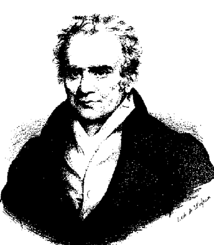
Figure 2. Gaspard Monge’s mesh-portrait obtained by mass transporting a uniform rectangular mesh into a “monitor” function.

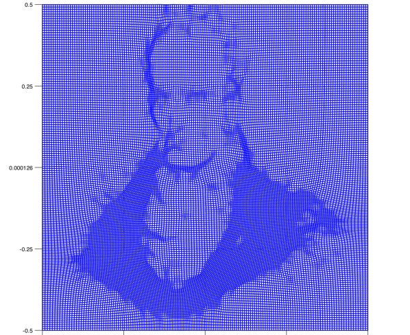
A bitmap of a portrait of Gaspard Monge, Lithography by F.S. Delpech (Public Domain)	$\mathbb{P}^{2}$ FE without gradient recovery
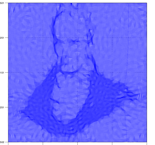
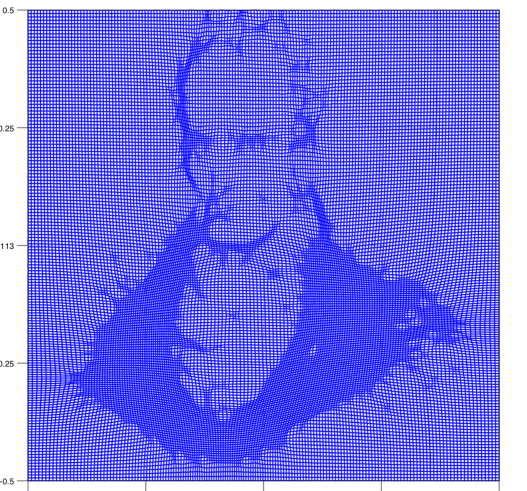
$\mathbb{P}^{1}$ FE with gradient recovery	$\mathbb{P}^{2}$ FE with gradient recovery
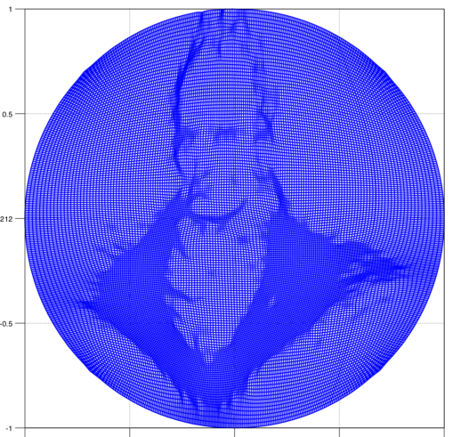
$\mathbb{P}^{2}$ FE without gradient recovery	$\mathbb{P}^{2}$ FE with gradient recovery

References

- Abgrall [2009] R. Abgrall. Construction of Simple, Stable, and Convergent High Order Schemes for Steady First Order Hamilton–Jacobi Equations. SIAM Journal on Scientific Computing, 31(4):2419–2446, Jan. 2009. ISSN 1064-8275. doi: 10.1137/040615997. URL http://epubs.siam.org/doi/abs/10.1137/040615997.
- Aguilera and Morin [2009] N. E. Aguilera and P. Morin. On convex functions and the finite element method. SIAM J. Numer. Anal., 47(4):3139–3157, 2009. ISSN 0036-1429. doi: 10.1137/080720917. URL http://epubs.siam.org/doi/10.1137/080720917.
- Barles and Souganidis [1991] G. Barles and P. E. Souganidis. Convergence of approximation schemes for fully nonlinear second order equations. Asymptotic Analysis, 4(3):271–283, 1991. doi: 10.3233/ASY-1991-4305. URL https://doi.dx.org/10.3233/ASY-1991-4305.
- Bellman [1997] R. Bellman. Introduction to matrix analysis, volume 19 of Classics in Applied Mathematics. Society for Industrial and Applied Mathematics (SIAM), Philadelphia, PA, 1997. ISBN 978-0-89871-399-2. URL http://www.worldcat.org/oclc/807510351. Reprint of the second (1970) edition, With a foreword by Gene Golub.
- Benamou et al. [2014] J.-D. Benamou, B. D. Froese, and A. M. Oberman. Numerical solution of the Optimal Transportation problem using the Monge–Ampère equation. Journal of Computational Physics, 260:107–126, Mar. 2014. ISSN 0021-9991. doi: 10.1016/j.jcp.2013.12.015. URL http://www.sciencedirect.com/science/article/pii/S0021999113008140.
- Brenier [1991] Y. Brenier. Polar factorization and monotone rearrangement of vector-valued functions. Communications on Pure and Applied Mathematics, 44(4):375–417, 6 1991. ISSN 1097-0312. doi: 10.1002/cpa.3160440402. URL http://onlinelibrary.wiley.com/doi/10.1002/cpa.3160440402/abstract/.
- Budd et al. [2013] C. J. Budd, M. J. P. Cullen, and E. J. Walsh. Monge–Ampére based moving mesh methods for numerical weather prediction, with applications to the Eady problem. Journal of Computational Physics, 236:247–270, Mar. 2013. ISSN 0021-9991. doi: 10.1016/j.jcp.2012.11.014. URL https://www.sciencedirect.com/science/article/pii/S0021999112006912.
- Budd et al. [2015] C. J. Budd, R. D. Russell, and E. J. Walsh. The geometry of r-adaptive meshes generated using optimal transport methods. Journal of Computational Physics, 282:113–137, 2015. ISSN 0021-9991. doi: 10.1016/j.jcp.2014.11.007. URL https://www.sciencedirect.com/science/article/pii/S0021999114007591.
- Caffarelli and Cabré [1995] L. A. Caffarelli and X. Cabré. Fully nonlinear elliptic equations, volume 43 of American Mathematical Society Colloquium Publications. American Mathematical Society, Providence, RI, 1995. ISBN 0-8218-0437-5. URL http://www.worldcat.org/oclc/246542992.
- Evans [2010] L. C. Evans. Partial differential equations, volume 19 of Graduate Studies in Mathematics. American Mathematical Society, Providence, RI, second edition, 2010. ISBN 978-0-8218-4974-3. URL http://www.worldcat.org/oclc/465190110.
- Feng and Jensen [2017] X. Feng and M. Jensen. Convergent semi-Lagrangian methods for the Monge-Ampère equation on unstructured grids. SIAM Journal on Numerical Analysis, 55(2):691–712, 2017. ISSN 0036-1429. doi: 10.1137/16M1061709. URL https://epubs.siam.org/doi/10.1137/16M1061709.
- Feng and Neilan [2014] X. Feng and M. Neilan. Finite element approximations of general fully nonlinear second order elliptic partial differential equations based on the vanishing moment method. Computers & Mathematics with Applications, 68(12, Part B):2182–2204, 12 2014. ISSN 0898-1221. doi: 10.1016/j.camwa.2014.07.023. URL https://dx.doi.org/10.1016/j.camwa.2014.07.023.
- Gallistl [2017a] D. Gallistl. Variational Formulation and Numerical Analysis of Linear Elliptic Equations in Nondivergence form with Cordes Coefficients. SIAM Journal on Numerical Analysis, 55(2):737–757, 01 2017a. ISSN 0036-1429. doi: 10.1137/16M1080495. URL https://epubs-siam-org/doi/10.1137/16M1080495.
- Gallistl [2017b] D. Gallistl. Numerical approximation of planar oblique derivative problems in nondivergence form. online preprint 2017/30, Karlsruhe Institute of Technology, KIT, Karlsruhe, Germany, 2017b. URL https://www.waves.kit.edu/downloads/CRC1173_Preprint_2017-30.pdf.
- Gilbarg and Trudinger [2001] D. Gilbarg and N. S. Trudinger. Elliptic partial differential equations of second order. Classics in Mathematics. Springer-Verlag, Berlin, 2001. ISBN 3-540-41160-7. URL http://www.worldcat.org/oclc/898241654. Reprint of the 1998 edition.
- Kawecki [2017a] E. Kawecki. A DGFEM for Nondivergence Form Elliptic Equations with Cordes Coefficients on Curved Domains. Technical report, arXiv, Aug. 2017a. URL http://arxiv.org/abs/1708.05028. arXiv: 1708.05028.
- Kawecki [2017b] E. Kawecki. A DGFEM for uniformly elliptic two dimensional oblique boundary value problems. online preprint 1711.01836, arXiv, Nov. 2017b. URL https://arxiv.org/abs/1711.01836.
- Kawecki et al. [2018] E. Kawecki, O. Lakkis, and T. Pryer. GitHub - ekawecki/Monge–Ampere, 08 2018. URL https://github.com/ekawecki/Monge--Ampere.
- Lakkis and Pryer [2011] O. Lakkis and T. Pryer. A finite element method for second order nonvariational elliptic problems. SIAM J. Sci. Comput., 33(2):786–801, 2011. ISSN 1064-8275. doi: 10.1137/100787672. URL https://arxiv.org/abs/1003.0292.
- Lakkis and Pryer [2013] O. Lakkis and T. Pryer. A finite element method for nonlinear elliptic problems. SIAM Journal on Scientific Computing, 35(4):A2025–A2045, 2013. doi: 10.1137/120887655. URL http://arxiv.org/abs/1103.2970.
- Lakkis and Pryer [2015] O. Lakkis and T. Pryer. An adaptive finite element method for the infinity Laplacian. In A. Abdulle, S. Deparis, D. Kressner, F. Nobile, and M. Picasso, editors, Numerical Mathematics and Advanced Applications - ENUMATH 2013, Lecture Notes in Computational Science and Engineering, pages 283–291. Springer International Publishing, Jan. 2015. ISBN 978-3-319-10704-2 978-3-319-10705-9. doi: 10.1007/978-3-319-10705-9˙28. URL http://arxiv.org/abs/1311.3930.
- Lieb and Loss [2001] E. H. Lieb and M. Loss. Analysis, volume 14 of Graduate Studies in Mathematics. American Mathematical Society, Providence, RI, second edition, 2001. ISBN 0-8218-2783-9. doi: 10.1090/gsm/014. URL http://dx.doi.org/10.1090/gsm/014.
- Lieberman [1987] G. M. Lieberman. Local estimates for subsolutions and supersolutions of oblique derivative problems for general second order elliptic equations. Transactions of the American Mathematical Society, 304(1):343–353, 1987. ISSN 0002-9947. doi: 10.2307/2000717. URL https://doi.org/10.2307/2000717.
- Lieberman [2001] G. M. Lieberman. Pointwise estimates for oblique derivative problems in nonsmooth domains. Journal of Differential Equations, 173(1):178–211, June 2001. ISSN 0022-0396. doi: 10.1006/jdeq.2000.3939. URL https://doi.org/10.1006/jdeq.2000.3939.
- Loeper and Rapetti [2005] G. Loeper and F. Rapetti. Numerical solution of the Monge–Ampère equation by a Newton’s algorithm. C. R. Math. Acad. Sci. Paris, 340(4):319–324, 2005. ISSN 1631-073X. doi: 10.1016/j.crma.2004.12.018. URL https://doi.org/10.1016/j.crma.2004.12.018.
- Logg et al. [2012] A. Logg, K.-A. Mardal, and G. N. Wells. Automated solution of differential equations by the finite element method, volume 84 of Lecture Notes in Computational Science and Engineering. Springer, Heidelberg, 2012. ISBN 978-3-642-23098-1; 978-3-642-23099-8. The FEniCS book.
- Neilan et al. [2017] M. Neilan, A. J. Salgado, and W. Zhang. Numerical analysis of strongly nonlinear PDEs *. Acta Numerica, 26:137–303, 05 2017. ISSN 0962-4929, 1474-0508. doi: 10.1017/S0962492917000071. URL https://www.cambridge.org/core/journals/acta-numerica/article/numerical-analysis-of-strongly-nonlinear-pdes/CB53724C153D209910B6EAA818E6B76D.
- Nochetto and Zhang [2018] R. H. Nochetto and W. Zhang. Discrete ABP Estimate and Convergence Rates for Linear Elliptic Equations in Non-divergence Form. Foundations of Computational Mathematics. The Journal of the Society for the Foundations of Computational Mathematics, 18(3):537–593, 2018. ISSN 1615-3375. doi: 10.1007/s10208-017-9347-y. URL https://mathscinet.ams.org/mathscinet-getitem?mr=3807356.
- Prins et al. [2014] C. R. Prins, J. H. M. Ten Thije Boonkkamp, J. van Roosmalen, W. L. Ijzerman, and T. W. Tukker. A Monge-Ampère-solver for free-form reflector design. SIAM Journal on Scientific Computing, 36(3):B640–B660, 2014. ISSN 1064-8275. doi: 10.1137/130938876. URL https://doi.org/10.1137/130938876.
- Pryer [2010] T. Pryer. Recovery techniques in finite element methods for evolution and nonlinear problems. Dphil in mathematics, University of Sussex, Brighton, England UK, September 2010. URL http://sro.sussex.ac.uk/6285/. funded by EPSRC DTA.
- Scott [1973] L. R. Scott. Finite-element techniques for curved boundaries. Phd thesis, Massachusetts Institute of Technology, 1973. URL http://gateway.proquest.com/openurl?url_ver=Z39.88-2004&rft_val_fmt=info:ofi/fmt:kev:mtx:dissertation&res_dat=xri:pqdiss&rft_dat=xri:pqdiss:0279379. Thesis (Ph.D.)–Massachusetts Institute of Technology.
- Smears and Süli [2013] I. Smears and E. Süli. Discontinuous galerkin finite element approximation of nondivergence form elliptic equations with cordès coefficients. SIAM Journal on Numerical Analysis, 51(4):2088–2106, 2013. doi: 10.1137/120899613. URL http://eprints.maths.ox.ac.uk/1623/.
- Urbas [1997] J. Urbas. On the second boundary value problem for equations of monge–ampère type. J. Reine Angew. Math., 487:115–124, 1997. ISSN 0075-4102. doi: 10.1515/crll.1997.487.115. URL https://www.degruyter.com/view/j/crll.1997.issue-487/crll.1997.487.115/crll.1997.487.115.xml.
- Villani [2003] C. Villani. Topics in optimal transportation, volume 58 of Graduate Studies in Mathematics. American Mathematical Society, Providence, RI, 2003. ISBN 0-8218-3312-X. URL http://www.worldcat.org/oclc/953518806.
- Zhang and Naga [2005] Z. Zhang and A. Naga. A new finite element gradient recovery method: superconvergence property. SIAM J. Sci. Comput., 26(4):1192–1213 (electronic), 2005. ISSN 1064-8275. doi: 10.1137/S1064827503402837. URL http://epubs.siam.org/doi/abs/10.1137/S1064827503402837.
- Zienkiewicz and Zhu [1987] O. C. Zienkiewicz and J. Z. Zhu. A simple error estimator and adaptive procedure for practical engineering analysis. Internat. J. Numer. Methods Engrg., 24(2):337–357, 1987. ISSN 0029-5981. doi: 10.1002/nme.1620240206. URL https://doi.org/10.1002/nme.1620240206.
- Zlámal [1977] M. Zlámal. Some superconvergence results in the finite element method. In I. Galligani and E. Magenes, editors, Mathematical aspects of finite element methods, volume 606 of Lecture Notes in Math., pages 353–362., Berlin, 1977. Proc. Conf., Consiglio Naz. delle Ricerche (C.N.R.), Rome, 1975, Springer. URL http://www.worldcat.org/oclc/771055099.
Index
- §2.1
- §2.2
- §2.1
- §2.1
- §1.2
- approximate domain §2.2
- benchmark solution §6
- best approximation §6
- degenerate elliptic on §4.3
- degenerate elliptic on §4.1
- degrees of freedom §2.2
- DOF §2.2
- domain transport condition §1.1
- double dot product §2.1
- elliptic on §4.1
- §6
- experimental order of convergence §6
- finite element convex with respect to §3.7
- fitted shape-regular triangulation §2.2
- Frobenius product §2.1
- generalised Hessian §3.2
- global discrete nonlinear operator §5.11
- gradient recovery §5.3
- (meshsize) §2.2
- §2.1
- incremental form §5.10
- Iverson–Knuth bracket §1.2
- §2.1
- lower uniform ellipticity constants §4.1
- §2.1
- MAOT §1.1
- meshsize §2.2
- modified Hessian recovery operator §5.10
- Monge–Ampère equation §1.1
- Monge–Ampère problem for optimal transport §1.1
- §2.2
- Newton–Raphson increment item 2
- Newton–Raphson iteration §4.4
- Newton–Raphson method §4.4
- next Newton–Raphson item 3
- nondivergence form item 1
- nonlinear second boundary value elliptic problem §1.2
- oblique derivative item 1
- optimal convergence rates §6
- partial differential equation §1.1
- PDE §1.1
- projection-based gradient recovery operator §5.4
- §2.1
- second boundary condition §1.1
- §2.1
- suboptimal convergence §6
- §2.1
- symmetric §2.1
- symmetric and positive definite §2.1
- §2.2
- trace §2.1, §2.1
- transport boundary condition §1.1
- transport field §1.1
- transport map §1.1
- transpose matrix §2.1
- upper uniform ellipticity constants §4.1
- wide-stencil finite difference §1.2
- §2.1
- §2.2