Thermal noise in non-boost-invariant dissipative hydrodynamics

Abstract

We study the effects of hydrodynamic fluctuations in non-boost-invariant longitudinal expansion of matter formed in relativistic heavy ion collisions. We formulate the theory of thermal noise within second-order viscous hydrodynamics treating noise as a perturbation on top of the non-boost-invariant flow. We develop a numerical simulation model to treat the (1+1)-dimension hydrodynamic evolution. The code is tested to reproduce the analytic results for the Riemann solver for expansion of matter in vacuum. For viscous hydrodynamic expansion, the initial energy density distribution are obtained by reproducing the measured charged hadron rapidity distribution at the RHIC energies. We show that the longitudinal rapidity correlations arising from space-time dependent thermal noise and from an induced thermal perturbation have distinct structures. In general, the rapidity correlations are found to be dominated by temperature fluctuations at small rapidity separation and velocity fluctuations at large rapidities. We demonstrate that thermal noise produce ridge-like two-particle rapidity correlations which persist at moderately large rapidities. The magnitude and pattern of the correlations are quite sensitive to various second-order dissipative formalisms and to the underlying equations of state, especially at large rapidities. The short-range part of the rapidity correlation is found to be somewhat enhanced as compared to that in boost-invariant flow of matter.

I Introduction

Relativistic dissipative hydrodynamic has become the state-of-the-art model to study the evolution of hot and dense matter formed at the Relativistic Heavy-ion Collider (RHIC) Adams:2005dq ; Adcox:2004mh and at the Large Hadron Collider (LHC) ALICE:2011ab ; ATLAS:2012at ; Chatrchyan:2013kba . Hydrodynamical model analysis of the large anisotropic flow observed in the plane transverse to the reaction plane has established the formation of a near-equilibrated strongly coupled Quark-Gluon-Plasma (QGP) with a small shear viscosity to entropy density ratio $\eta_{v}/s$. The flow is found to originate mostly during the initial stages of dynamical evolution Huovinen:2001cy ; Heinz:2001xi . Considerable efforts are underway for an accurate determination of the transport properties of the QGP formed.

Inspite of the success of hydrodynamic models in the description of relativistic heavy-ion collisions, considerably uncertainty prevails. This relates to the formulation of dissipative hydrodynamics, the correct initial conditions, and the numerical implementation. At present the models used are commonly based on approaches, such as the second-order dissipative (causal) equations in the Müller-Israel-Stewart (MIS) framework Muller:1967zza ; Israel:1979wp ; Muronga:2003ta ; Romatschke:2007mq , the Chapman-Enskog- (CE-) like iterative expansion of the Boltzmann equation in the relaxation-time approximation Jaiswal:2013npa ; Bhalerao:2013pza ; Chattopadhyay:2014lya , the second-order viscous hydrodynamics from AdS/CFT correspondence, and the anisotropic hydrodynamics Strickland:2014eua ; Heinz:2014zha . For a reasonable description of the flow data, all these models require a very early thermalization proper time of $\tau\approx 0.2-0.6$ fm/c, that, hitherto, lacks a proper explanation.

One of the major uncertainties in the hydrodynamic model extraction of $\eta_{v}/s$ lies with the initial state models. In fact, viscous hydrodynamic descriptions with different initial conditions, can be made compatible with the data for elliptic ($n=2$) and triangular ($n=3$) flow harmonics $v_{n}=\langle\cos(n-\Psi_{n})\rangle$, for different tuned values of $\eta_{v}/s$ Luzum:2008cw ; Schenke:2011bn ; Qiu:2011hf . While the elliptic flow is driven primarily by the hydrodynamic response of the initial overlap geometry of the colliding nuclei, the odd harmonics are solely governed by the initial-state fluctuations of the nucleon position in the nuclei Alver:2010gr . Pre-equilibrium parton dynamics and fluctuations in the parton production and scattering was shown to have a crucial effect on the final anisotropic flow Gale:2012rq ; Bhalerao:2015iya ; Chattopadhyay:2017bjs . Further sources of fluctuations pertain to energy deposition (and its evolution) by a partonic jet propagating in the hydrodynamic medium Staig:2010pn and the treatment of particilization of the fluid cells at freeze-out Tachibana:2017syd .

In contrast, hydrodynamic fluctuations arising due to intrinsic thermal (and particle number) fluctuations in each fluid cell occur during the entire evolution of the system Kapusta:2011gt ; Young:2013fka ; Kapusta:2014dja ; Young:2014pka ; Albright:2015uua ; Nagai:2016wyx . Based on the fluctuation-dissipation theorem, it is natural, that any dissipative system close to thermal equilibrium should should exhibit thermal fluctuations. In heavy-ion collisions, as the transverse size of the participant zone is about 5-10 fm, and the evolution stage lasts for about $\tau\approx 10$ fm/c, thermal fluctuations in the fluid medium could have measurable and important consequences. The formulation of hydrodynamic fluctuations in the nonrelativistic limit Landau was recently extended to relativistic hydrodynamic regime. As an application of the stochastic thermal noise in relativistic heavy-ion collisions, it was demonstrated within boost-invariant one-dimensional (Bjorken) expansion of the fluid, that the two-particle rapidity correlations exhibit ridge-like structures observed in collisions at RHIC and LHC Kapusta:2011gt .

The thermal fluctuation of the energy-momentum tensor $\Xi^{\mu\nu}$ has a nontrivial autocorrelation $\langle\Xi^{\mu\nu}(x)\Xi^{\alpha\beta}(x^{\prime})\rangle\sim T\eta_{v}\>\delta^{4}(x-x^{\prime})$ Kapusta:2011gt ; Young:2013fka . Due to the Dirac-delta function, the energy and momentum density averaged value of this white noise becomes $\sim 1/\sqrt{\Delta V\Delta t}$. Thus even for small shear viscosities, the white noise sets a lower limit on the system cell size $\Delta V$ that is essentially comparable to the correlation length. Consequently, white noise could lead to large gradients which makes the basic hydrodynamic formulation (based on gradient expansion) questionable. One possible way to overcome this is by using thermal fluctuations nonperturbatively via colored noise Kapusta:2014dja . Alternatively, white noise can be implemented by treating fluctuations as perturbations (in a linearized hydrodynamic framework) on top of a baseline non-fluctuating hydrodynamic evolution Kapusta:2011gt ; Young:2013fka ; Chattopadhyay:2017rgh . While analytic solution of hydrodynamic fluctuation exists within relativistic Navier-Stokes theory (for a conformal fluid) with idealized boost-invariant dynamics in Bjorken flow Kapusta:2011gt and Gubser flow Yan:2015lfa , numerical simulations of thermal fluctuation were performed for various second-order dissipative hydrodynamics for Bjorken flow profiles Chattopadhyay:2017rgh .

It is however important to realize that the propagation of the fluctuations over large distances and times critically depend on the underlying expansion of the fluid. As compared to a static fluid Landau , the observables related to the fluctuations, (namely, the two-particle rapidity correlations and harmonic flow $v_{n}$ distributions), calculated at the freeze-out time (or temperature), would have different features. The thermal noise correlators have been calculated and their phenomenological applications for the boost-invariant (Bjorken) expansion of matter have been explored Kapusta:2011gt ; Chattopadhyay:2017rgh . However, the longitudinal boost-invariant scenario could only give a reasonable description for the midrapidity region during the initial stages of relativistic heavy ion collisions Bjorken:1982qr . At large rapidities and due to finite size of the expanding fluid, thermal noise would exhibit a different behavior. As a matter of fact, even the noiseless non-boost-invariant longitudinal expansion could create large velocity and energy gradients at the cell boundaries near large space-time rapidities that may severely affect the baseline hydrodynamic evolution Ryblewski:2010bs ; Martinez:2010sd ; Florkowski:2016kjj .

In this paper, we formulate the hydrodynamic (thermal) fluctuation in the non-boost-invariant (1+1)D longitudinal expansion of viscous matter within the Müller-Israel-Stewart and Chapman-Enskog theories. For the perturbative application of the white noise, we have developed a (1+1)D viscous hydrodynamic simulation in the Milne coordinates ($\eta,\tau$) that is suitable to study relativistic heavy-ion collisions. The code has been tested for stability against shock waves across the cell boundaries and at large rapidities by comparing with the Riemann and Landau-Khalatnikov wave solutions. Within linearized second-order viscous hydrodynamic framework, we treat the fluctuations as perturbation on top of the background (1+1)D expanding viscous medium. We first consider a single thermal perturbation and explore the resulting longitudinal rapidity-correlations to gain insight into the more complex case of thermal noise generated at all space-time points. We then perform extensive numerical simulation of hydrodynamic fluctuations and study the rapidity correlations for the commonly used hydrodynamics dissipative theories, namely MIS and CE formalisms and for the conformal and lattice QCD equation of state (EoS). In particular, we will show that distinct magnitude and structures in the rapidity correlations are obtained for these different cases.

The paper is organized as follows. In Sec. II we formulate the theory of hydrodynamic fluctuations in the linearized limit for non-boost-invariant hydrodynamic expansion of viscous fluid. We derive analytical expressions for the two-particle rapidity correlations from thermal noise at freeze-out. In Sec. III A we test the (1+1)D hydrodynamic code with simple wave solutions. We then constrain in Sec. III B the initial conditions of the viscous hydrodynamic code from fits to the measured rapidity distribution of hadrons in central Au+Au collisions at RHIC. With these parameter sets we present results for various rapidity correlators from an induced thermal fluctuation and thermal noise in Sec. III C and III D, respectively. In Sec. III E the results for rapidity correlations due to thermal noise are compared for the MIS and CE viscous approaches and for various EoS. A summary and conclusions are presented in Sec. IV.

II Thermal noise in relativistic hydrodynamics

II.1 Fluctuation-dissipation relations for causal second-order theories

The hydrodynamic evolution of a system is governed by the conservation equations for particle current, $\partial_{\mu}N^{\mu}=0$, and the energy-momentum tensor, $\partial_{\mu}T^{\mu\nu}=0$, where

$$N^{\mu} =nu^{\mu}+n^{\mu},$$

$$T^{\mu\nu} =\epsilon u^{\mu}u^{\nu}-(p+\Pi)\Delta^{\mu\nu}+\pi^{\mu\nu}.$$ (1)

Here $n$ is the number density, $\epsilon$ and $p$ are respectively the energy density and pressure in the fluid’s local rest frame (LRF), $\pi^{\mu\nu}$ is the shear pressure tensor, $n^{\mu}$ is the particle diffusion current and $\Pi$ the local bulk viscous pressure. $\Delta^{\mu\nu}=g^{\mu\nu}-u^{\mu}u^{\nu}$ is the projection operator on the three-space orthogonal to the hydrodynamic four-velocity $u^{\mu}$ in the LRF that is defined by the Landau-matching condition $T^{\mu\nu}u_{\nu}=\epsilon u^{\mu}$. We will disregard particle flow $N^{\mu}$, which is a reasonable approximation due to very small values of net-baryon number formed at RHIC and LHC.

In the relativistic Navier-Stokes (first order) theory, the instantaneous constituent equations for the bulk and shear pressures are

$$\Pi_{{NS}}=-\zeta\nabla\cdot u,~{}~{}~{}\pi_{NS}^{\mu\nu}=2\eta_{v}\nabla^{\langle u}u^{\nu\rangle},$$ (2)

where the transport coefficients $\zeta,\eta_{v}\geq 0$ are the bulk and shear viscosity, and $\nabla^{\langle u}u^{\nu\rangle}=(\nabla^{\mu}u^{\nu}+\nabla^{\nu}u^{\mu})/2-(\nabla\cdot u)\Delta^{\mu\nu}/3$ and $\nabla^{\mu}=\Delta^{\mu\nu}\partial_{\nu}$. In the MIS theory Muller:1967zza ; Israel:1979wp ; Muronga:2003ta ; Romatschke:2007mq , derived from positivity of entropy four-current divergence, the second-order dissipative hydrodynamic equations,

$$D\Pi =-\frac{1}{\tau_{\Pi}}\left(\Pi+\zeta\nabla\cdot u\right),$$

$$\Delta^{\mu\nu}_{\alpha\beta}D\pi^{\alpha\beta} \approx-\frac{1}{\tau_{\pi}}\left(\pi^{\mu\nu}-2\eta_{v}\nabla^{\langle u}u^{\nu\rangle}\right)-\frac{4}{3}\pi^{\mu\nu}\theta,$$ (3)

restore causality by enforcing the bulk and shear pressures to relax to their first-order values via the relaxation times $\tau_{\Pi}=\zeta\beta_{0}$ and $\tau_{\pi}=2\eta_{v}\beta_{2}$; where $\beta_{0}$ and $\beta_{2}$ are second-order transport coefficients in the entropy current. $D=u\cdot\partial$ is the time derivative in the local comoving frame and $\theta=\nabla\cdot u$ is the local expansion rate. In the following, we shall neglect the bulk viscosity which has negligibly small values at all temperatures, other than at the critical temperature $T_{c}=170$ MeV for deconfinement transition.

For the dissipative equation, we shall also consider the second-order equation for shear tensor in the Chapman-Enskog approach obtained by iteratively solving the Boltzmann equation in relaxation time approximation Jaiswal:2013npa ; Bhalerao:2013pza ; Chattopadhyay:2014lya ,

$$\dot{\pi}^{\langle\mu\nu\rangle}\!+\frac{\pi^{\mu\nu}}{\tau_{\pi}}\!=2\beta_{\pi}\sigma^{\mu\nu}\!+2\pi_{\gamma}^{\langle\mu}\omega^{\nu\rangle\gamma}\!-\frac{10}{7}\pi_{\gamma}^{\langle\mu}\sigma^{\nu\rangle\gamma}\!-\frac{4}{3}\pi^{\mu\nu}\theta,$$ (4)

where the vorticity $\omega^{\mu\nu}\equiv(\nabla^{\mu}u^{\nu}-\nabla^{\nu}u^{\mu})/2$ and $\beta_{\pi}=4p/5$.

The total energy-momentum (ignoring bulk viscosity) in presence of a noise tensor $\Xi^{\mu\nu}$ is,

$$T^{\mu\nu}=\epsilon u^{\mu}u^{\nu}-p\Delta^{\mu\nu}+\pi^{\mu\nu}+\Xi^{\mu\nu},$$ (5)

where $\Xi^{\mu\nu}(x)$ is a stochastic field in space-time with ensemble average $\langle\Xi^{\mu\nu}(x)\rangle=0$. The auto-correlation $\langle\Xi^{\mu\nu}(x_{1})\Xi^{\alpha\beta}(x_{2})\rangle$ is derived using the fluctuation-dissipation theorem and depends on the form of evolution equation of the shear stress tensor. We use the theory of quasi-stationary fluctuations Landau in which one considers the set of time evolution equations for the variables $x_{a}$,

$$\dot{x}_{a}=-\sum_{a}\gamma_{ab}X_{b}+y_{a}.$$ (6)

$X_{b}$ are “driving” forces, $y_{a}$ are random fluctuations. The rate of change of entropy $S(x_{a})$ is given by

$$\dot{S}=-\sum_{a}\dot{x}_{a}X_{a},$$ (7)

where $X_{a}=-\partial S/\partial x_{a}$. As the probability of fluctuating variables in thermal equilibrium must be $e^{S}$, the autocorrelation of the noise should have the form,

$$\langle y_{a}(t_{1})y_{b}(t_{2})\rangle=(\gamma_{ab}+\gamma_{ba})\delta(t_{1}-t_{2}).$$ (8)

The fluctuation-dissipation relation in viscous hydrodynamics can be derived using the above formalism Kapusta:2011gt ; Chattopadhyay:2017rgh ; Kumar:2013twa . For the MIS theory, the expression for second-order entropy four-current is given by,

$$S^{\mu}=su^{\mu}-\frac{\beta_{2}}{2T}u^{\mu}\pi^{\alpha\beta}\pi_{\alpha\beta},$$ (9)

where $s=(\epsilon+p)/T$ and $\beta_{2}=1/(2\beta_{\pi})$. Using the temporal-component of $\partial_{\mu}S^{\mu}$, we obtain the rate of change of entropy,

$$\frac{dS}{dt}=\int d^{3}\!x\frac{\pi^{\mu\nu}}{T}\left[\nabla_{\mu}u_{\nu}-\beta_{2}\dot{\pi}_{\mu\nu}-\beta_{2}\frac{4}{3}\theta\pi_{\mu\nu}\right].$$ (10)

In analogy to Eq. (7) we identify

$$\dot{x}_{a}\to \pi^{\mu\nu},$$ (11)

$$X_{a}\to -\frac{1}{T}\left[\nabla_{\mu}u_{\nu}-\beta_{2}\dot{\pi}_{\mu\nu}-\beta_{2}\lambda_{\pi}\theta\pi_{\mu\nu}\right]\,\,\Delta V\equiv X_{\mu\nu}.$$ (12)

As in Eq. (6), we add a stochastic tensor $\xi^{\mu\nu}$ to the shear stress tensor,

$$\pi^{\mu\nu} =-\gamma^{\mu\nu\alpha\beta}X_{\alpha\beta}+\xi^{\mu\nu},$$ (13)

where $\gamma^{\mu\nu\alpha\beta}$ should yield the shear tensor expression of Eq. (II.1) on contraction with $X_{\alpha\beta}$. Due to symmetries of $\pi^{\mu\nu}$, we have $\gamma^{\mu\nu\alpha\beta}=\gamma^{\nu\mu\alpha\beta}$, $\gamma^{\mu\alpha\beta}_{\mu}=0$, and $\gamma^{\mu\nu\alpha\beta}u_{\mu}=0$. Note that the identification of $X_{\mu\nu}$ is not unique as the transformation $X_{\mu\nu}\to X_{\mu\nu}+H_{\mu\nu}$, keeps $dS/dt$ invariant if $H_{\mu\nu}$ is orthogonal to $\pi^{\mu\nu}$. We thus have to find an autocorrelation which is insensitive to such transformations, namely, $\gamma^{\mu\nu\alpha\beta}=\gamma^{\mu\nu\beta\alpha}$, $\gamma^{\mu\nu\alpha}_{\alpha}=0$, and $\gamma^{\mu\nu\alpha\beta}u_{\alpha}=0$.

The form of $\gamma^{\mu\nu\alpha\beta}$ consistent with the constraints is,

$$\gamma^{\mu\nu\alpha\beta}= 2\eta_{v}T\Delta^{\mu\nu\alpha\beta}.$$ (14)

Correspondingly one obtains the noise autocorrelation in the MIS theory to be Chattopadhyay:2017rgh :

$$\langle\xi^{\mu\nu}(x)\xi^{\alpha\beta}(x^{\prime})\rangle= 4\eta_{v}T\Delta^{\mu\nu\alpha\beta}\delta^{4}(x-x^{\prime}).$$ (15)

We now present the fluctuation-dissipation relation for Chapman-Enskog case. The entropy four-current obtained from Boltzmann’s H-theorem has the expression as of Eq. (9), see Ref. Chattopadhyay:2014lya . Following the same procedure as above, the form of $\gamma^{\mu\nu\alpha\beta}$ for the Chapman-Enskog case is,

$$\gamma^{\mu\nu\alpha\beta}= 2\eta_{v}T\Big{(}\Delta^{\mu\nu\alpha\beta}-\frac{10}{7}\beta_{2}\Delta^{\mu\nu}_{\zeta\kappa}\pi^{\zeta}_{\gamma}\Delta^{\kappa\gamma\alpha\beta}$$

$$+2\tau_{\pi}\Delta^{\mu\nu}_{\zeta\kappa}\omega^{\zeta}_{\gamma}\Delta^{\kappa\gamma\alpha\beta}\Big{)}.$$ (16)

Consequently, one obtains the noise autocorrelation in the Chapman-Enskog theory to be Chattopadhyay:2017rgh :

$$\langle\xi^{\mu\nu}(x)\xi^{\alpha\beta}(x^{\prime})\rangle= 4\eta_{v}T\Big{(}\Delta^{\mu\nu\alpha\beta}-\frac{5}{7}\beta_{2}\Delta^{\mu\nu}_{\zeta\kappa}\pi^{\zeta}_{\gamma}\Delta^{\kappa\gamma\alpha\beta}$$

$$-\frac{5}{7}\beta_{2}\Delta^{\alpha\beta}_{\zeta\kappa}\pi^{\zeta}_{\gamma}\Delta^{\kappa\gamma\mu\nu}$$

$$+\omega-{\rm terms}\Big{)}\delta^{4}(x-x^{\prime}).$$ (17)

As opposed to the MIS case where the auto-correlation function in the fluid rest frame depends only on the coefficient of shear viscosity $\eta_{v}$ and temperature, the above result shows that the auto-correlation function of thermal noise in Chapman-Enskog scenario is sensitive to components of shear stress tensor as well as vorticity.

It is important to note that in the derivation of fluctuation-dissipation relation using the theory of quasi-stationary fluctuations, the noise tensor $\xi^{\mu\nu}$ should be added to the shear evolution equation. However, by defining $\pi^{\prime\mu\nu}\equiv\pi^{\mu\nu}-\Xi^{\mu\nu}$, so as to obtain the same form as in Eq. (5), we get a relaxation-type evolution of $\Xi^{\mu\nu}$, which essentially implies that $\Xi^{\mu\nu}$ becomes a colored-noise (correlated over space-times), as opposed to its uncorrelated (white-noise) structure in the first-order Navier-Stokes theory Kapusta:2011gt . In the MIS theory, we have the equation of motion of the noise tensor $\Xi^{\mu\nu}$,

$$\dot{\Xi}^{\langle\mu\nu\rangle}=-\frac{1}{\tau_{\pi}}\left(\Xi^{\mu\nu}-\xi^{\mu\nu}\right)-\frac{4}{3}\Xi^{\mu\nu}\theta,$$ (18)

and for the CE equation we get

$$\dot{\Xi}^{\langle\mu\nu\rangle}=-\frac{1}{\tau_{\pi}}\left(\Xi^{\mu\nu}-\xi^{\mu\nu}\right)+2\pi_{\gamma}^{\langle\mu}\omega^{\nu\rangle\gamma}-\frac{10}{7}\Xi^{\langle\mu}_{\gamma}\sigma^{\nu\rangle\gamma}-\frac{4}{3}\Xi^{\mu\nu}\theta.$$ (19)

In the following, we shall linearize the stochastic hydrodynamic equations about a background (averaged) solution such that the r.h.s of Eqs. (15) and (II.1) will be computed using these averaged solutions. Considering fluctuations in temperature (or energy density), flow velocity and shear pressure tensor Kapusta:2011gt , their values in the linearized limit can be written as

$$\epsilon =\epsilon_{0}+\delta\epsilon\equiv\epsilon_{0}+\epsilon_{1},$$

$$u^{\mu} =u_{0}^{\mu}+\delta u^{\mu}\equiv u_{0}^{\mu}+u_{1}^{\mu},$$

$$\pi^{\mu\nu} =\pi_{0}^{\mu\nu}+\delta\pi^{\mu\nu}\equiv\pi_{0}^{\mu\nu}+\pi_{1}^{\mu\nu}.$$ (20)

The subscript “0” corresponds to the average (noiseless) values of the quantities whose evolution will be described in Sec. II B. The equations for fluctuations (denoted by subscript “1”) are presented in Sec. II C. As a consequence of Eq. (II.1), the total energy-momentum tensor of Eq. (5) can be decomposed into $T^{\mu\nu}=T_{0}^{\mu\nu}+T_{1}^{\mu\nu}$, consisting of a noiseless part $T_{0}^{\mu\nu}$ and a fluctuating part $\delta T^{\mu\nu}\equiv T_{1}^{\mu\nu}$.

II.2 (1+1)D non-boost-invariant viscous hydrodynamic

In the present calculation for non-boost-invariant longitudinal expansion, the hydrodynamic equations effectively correspond to (1+1)D. For high-energy collisions at RHIC and LHC, the space-time evolution can be conveniently described in the Milne coordinates of longitudinal proper time $\tau=\sqrt{t^{2}-z^{2}}$ and space-time rapidity $\eta=\ln[(t+z)/(t-z)]/2$. In ($\tau,x,y,\eta$) coordinates, the metric tensor becomes $g^{mn}={\rm diag}(1,-1,-1,-1/\tau^{2})$. Due to the translational and rotational invariance in the transverse plane, the four-velocity can be parametrized as $u_{0}^{\mu}=(u_{0}^{\tau},u_{0}^{x},u_{0}^{y},u_{0}^{\eta})\equiv\gamma_{0}(1,0,0,v_{\eta_{0}})$, where $\gamma_{0}=1/\sqrt{1-\tau^{2}v_{\eta_{0}}^{2}}$ arises from the normalization condition $u_{0}^{\mu}u_{0\mu}=1$. The nonvanishing components of the Christoffel symbols are $\Gamma^{\eta}_{\eta\tau}=\Gamma^{\eta}_{\tau\eta}=1/\tau$ and $\Gamma^{\tau}_{\eta\eta}=\tau$. The time derivative in the local fluid rest frame and the local expansion rate are then

$$D_{0} =u_{0}\cdot\partial=\gamma_{0}\left(\partial_{\tau}+v_{\eta_{0}}\partial_{\eta}\right),$$ (21)

$$\theta_{0} =\partial\cdot u_{0}=\frac{1}{\tau}\partial_{\tau}(\tau\gamma_{0})+\partial_{\eta}(\gamma_{0}v_{\eta_{0}}).$$ (22)

Due to constraints on $\pi_{0}^{\mu\nu}$, namely, orthogonality to $u_{0}^{\mu}$ (i.e. $\pi_{0}^{mn}u_{0_{m}}=0$), tracelessness ($\pi_{0}^{mn}g_{mn}=0$), and azimuthal ($x-y$) symmetry, there is only one independent component which we take to be $\pi_{0}^{\eta\eta}$. The other non-vanishing components can be expressed in terms of $\pi_{0}^{\eta\eta}$ as,

$$\pi_{0}^{\tau\tau} =\tau^{4}v_{\eta_{0}}^{2}\pi_{0}^{\eta\eta},~{}~{}\pi_{0}^{\tau\eta}=\tau^{2}v_{\eta_{0}}\pi_{0}^{\eta\eta},~{}~{}$$

$$\pi_{0}^{xx} =\pi_{0}^{yy}=-\frac{\tau^{2}}{2\gamma_{0}^{2}}\pi_{0}^{\eta\eta}.$$ (23)

The two independent components of the noiseless part of energy-momentum tensor $T_{0}^{\mu\nu}$ in the global frame reduce to

$$T_{0}^{\tau\tau} =(\epsilon_{0}+p_{0})\gamma_{0}^{2}-p_{0}+\pi_{0}^{\tau\tau}=(\epsilon_{0}+{\cal P}_{0})\gamma_{0}^{2}-{\cal P}_{0},$$ (24)

$$T_{0}^{\tau\eta} =(\epsilon_{0}+p_{0})\gamma_{0}^{2}v_{\eta_{0}}+\pi_{0}^{\tau\eta}=(\epsilon_{0}+{\cal P}_{0})\gamma_{0}^{2}v_{\eta_{0}},$$ (25)

where Eq. (II.2) has been used to obtain the right-hand-side of the second equality. The effective (longitudinal) pressure is denoted as ${\cal P}_{0}=p_{0}+\tau^{2}\pi_{0}^{\eta\eta}/\gamma_{0}^{2}$. Using $T_{0}^{\eta\eta}=[(\epsilon_{0}+{\cal P}_{0})\gamma_{0}^{2}-\epsilon_{0}]/\tau^{2}$ the equation of motion $T^{mn}_{;m}=0$ for the $n=\tau$ and $n=\eta$ component can be written as

$$\partial_{\tau}(\tilde{T}_{0}^{\tau\tau})+\partial_{\eta}(\tilde{v}_{\eta_{0}}\tilde{T}_{0}^{\tau\tau})=-\left(\epsilon_{0}+{\cal P}_{0}\right)\gamma_{0}^{2}+\epsilon_{0},$$ (26)

$$\partial_{\tau}(\tilde{T}_{0}^{\tau\eta})+\partial_{\eta}(v_{\eta_{0}}\tilde{T}_{0}^{\tau\eta}+\tilde{\cal P}_{0}/\tau^{2})=-2\left(\epsilon_{0}+{\cal P}_{0}\right)\gamma_{0}^{2}v_{\eta_{0}}.$$ (27)

Here we have used the shorthand notation $\tilde{A}^{mn}=\tau A^{mn}$ and $\tilde{v}_{\eta_{0}}=\tilde{T}_{0}^{\tau\eta}/\tilde{T}_{0}^{\tau\tau}=T_{0}^{\tau\eta}/T_{0}^{\tau\tau}$.

In order to write the evolution equation for $\pi_{0}^{\eta\eta}$, we obtain the general form of relaxation equation for the full tensor $\dot{\pi}^{\langle\eta\eta\rangle}$. Using the orthogonality conditions $\pi^{\mu\nu}u_{\nu}=0$ and $\dot{u}^{\mu}u_{\mu}=0$, the comoving derivative of $\pi^{\eta\eta}$ in (1+1)D can be expressed in a compact form,

$$\dot{\pi}^{\langle\eta\eta\rangle}=\frac{\gamma^{2}}{\tau^{2}}u^{\mu}\partial_{\mu}\left(\frac{\tau^{2}\pi^{\eta\eta}}{\gamma^{2}}\right).$$ (28)

Moreover, using $\sigma^{\eta\eta}=-(2/3)(\gamma^{2}\theta/\tau^{2})$ and defining the total (background plus noise) shear stress $\pi=-\tau^{2}\pi^{\eta\eta}/\gamma^{2}$, the MIS Eq. (II.1) on adding the noise term $\xi^{\mu\nu}$ can be written as

$$u^{\mu}\partial_{\mu}\pi=-\frac{1}{\tau_{\pi}}\left(\pi+\frac{\tau^{2}}{\gamma^{2}}\xi^{\eta\eta}-\frac{4}{3}\eta_{v}\>\theta\right)-\lambda_{\pi}\pi\>\theta.$$ (29)

Here the coefficient $\lambda_{\pi}=4/3$ in this MIS dissipative equation. The evolution equation for the background shear stress component $\pi_{0}\equiv-\tau^{2}\pi_{0}^{\eta\eta}/\gamma_{0}^{2}$ then has the form,

$$u_{0}^{\mu}\partial_{\mu}\pi_{0}=-\frac{1}{\tau_{\pi}}\left(\pi_{0}-\frac{4}{3}\eta_{v}\>\theta_{0}\right)-\lambda_{\pi}\pi_{0}\>\theta_{0}.$$ (30)

For the CE case the dissipative equation (4) in (1+1)D has the same form as Eq. (29) with $\lambda_{\pi}=38/21$.

The three evolution Eqs. (26), (27), (30) in four unknowns are closed with the equation of state $p=p(\epsilon)$. Using Eqs. (24)-(25), one can express the energy density and the (longitudinal) velocity as

$$\epsilon_{0} =T_{0}^{\tau\tau}-\tau^{2}v_{\eta_{0}}T_{0}^{\tau\eta},$$ (31)

$$v_{\eta_{0}} =\frac{T_{0}^{\tau\eta}}{T_{0}^{\tau\tau}+p_{0}\left(\epsilon_{0}=T_{0}^{\tau\tau}-\tau^{2}v_{\eta_{0}}T_{0}^{\tau\eta}\right)-\pi_{0}},$$ (32)

and these allow one to extract $v_{\eta_{0}}$ by one-dimensional zero-search. The above set of evolution equations are solved using SHASTA-FCT algorithm.

II.3 Thermal fluctuations in non-boost-invariant viscous hydrodynamics

We will now obtain the linearized hydrodynamic equations for thermal fluctuations in the non-boost-invariant (1+1)D expansion of matter within MIS formulation. Substituting the first-order fluctuations of Eq. (II.1) into the total energy-momentum tensor:

$$T^{\mu\nu} =\epsilon u^{\mu}u^{\nu}-p\Delta^{\mu\nu}+\pi^{\mu\nu},$$

$$=T_{0}^{\mu\nu}+\delta T_{\rm id}^{\mu\nu}+\delta\pi^{\mu\nu}=T_{0}^{\mu\nu}+T_{1}^{\mu\nu},$$ (33)

where $T_{0}^{\mu\nu}$ is the noiseless energy-momentum tensor whose evolution equations has been obtained in Sec. II B. Note that the noise term $\xi^{\mu\nu}$ has been included in the shear evolution Eq. (29). The fluctuating part of the ideal energy-momentum tensor is $\delta T_{\rm id}^{\mu\nu}=\delta(\epsilon u^{\mu}u^{\nu}-p\Delta^{\mu\nu})$, and can be determined by the fluctuating variables ($\delta\epsilon,\delta u^{\mu},\delta p$). The conservation equations for the total energy-momentum tensor, $\partial_{\mu}T^{\mu\nu}=0$, along with that for the average part, $\partial_{\mu}T_{0}^{\mu\nu}=0$, lead to

$$\partial_{\mu}(\delta T_{\rm id}^{\mu\nu}+\delta\pi^{\mu\nu})\equiv\partial_{\mu}(\delta T^{\mu\nu})=0.$$ (34)

The above equations are combined to yield

$$\delta T^{\mu\nu}\equiv T_{1}^{\mu\nu}= \epsilon_{1}u_{0}^{\mu}u_{0}^{\nu}+\epsilon_{0}u_{1}^{\mu}u_{0}^{\nu}+\epsilon_{0}u_{0}^{\mu}u_{1}^{\nu}$$

$$-p_{0}\Delta_{1}^{\mu\nu}-p_{1}\Delta_{0}^{\mu\nu}+\pi_{1}^{\mu\nu}.$$ (35)

While the event-averaged fluctuations yield $\langle\delta T^{\mu\nu}\rangle=0$, thermal noise $\xi^{\mu\nu}$ induces a nonvanishing $\langle\delta T^{\mu\nu}\delta T^{\alpha\beta}\rangle$ which was demonstrated to result in the two-particle rapidity correlation Kapusta:2011gt and affect the event-by-event fluctuation of elliptic flow Young:2014pka .

On imposing the orthonormality condition of the total four-velocity of the fluid, i.e. $u^{\mu}u_{\mu}=(u_{0}^{\mu}+u_{1}^{\mu})(u_{0\mu}+u_{1\mu})=1$ and noting that $u_{0}^{\mu}u_{0\mu}=1$, we get in the linearized limit

$$u_{1}^{\tau}=\tau^{2}u_{1}^{\eta}v_{\eta_{0}}.$$ (36)

Further, by using the orthogonality of the total shear pressure with four-velocity, $\pi^{\mu\nu}u_{\nu}=0$, and the corresponding Eq. (II.2) for the noiseless part, one gets for the fluctuating shear stress component

$$\pi_{1}^{\mu\nu}u_{0\nu}=-\pi_{0}^{\mu\nu}u_{1\nu}.$$ (37)

Making use of these conditions, together with the tracelessness of $\pi^{\mu\nu}$ and Eqs. (II.2), we obtain for the (1+1)D expansion,

$$\pi_{1}^{\tau\tau} =\tau^{4}v_{\eta_{0}}^{2}\pi_{1}^{\eta\eta}-2\frac{\tau^{2}v_{\eta_{0}}u^{\eta}_{1}}{\gamma_{0}}\pi_{0},$$

$$\pi_{1}^{\tau\eta} =\tau^{2}\pi_{1}^{\eta\eta}v_{\eta_{0}}-\frac{u^{\eta}_{1}}{\gamma_{0}}\pi_{0}.$$ (38)

The corresponding fluctuating components of the energy-momentum tensor of Eq. (II.3) is then:

$$T_{1}^{\tau\tau} =(\epsilon_{1}+\tau^{2}{\cal P}_{1})\gamma_{0}^{2}-\tau^{2}{\cal P}_{1}+\tau^{2}u_{1}^{\eta}v_{\eta_{0}}\gamma_{0}{\cal U}_{0}(2-\tau^{2}v_{\eta_{0}}^{2}),$$

$$T_{1}^{\tau\eta} =(\epsilon_{1}+\tau^{2}{\cal P}_{1})\gamma_{0}^{2}v_{\eta_{0}}+u_{1}^{\eta}\gamma_{0}{\cal U}_{0},$$

$$T_{1}^{\eta\eta} =T_{1}^{\tau\eta}v_{\eta_{0}}+{\cal P}_{1}.$$ (39)

We use the definition ${\cal P}_{1}=u_{1}^{\eta}v_{\eta_{0}}{\cal U}_{0}/\gamma_{0}+{\cal V}_{1}/\tau^{2}$ with ${\cal U}_{0}=\epsilon_{0}+p_{0}-\pi_{0}$ and ${\cal V}_{1}=p_{1}-\pi_{1}$. Here $\pi_{1}\equiv-(\tau^{2}/\gamma_{0}^{2})\pi_{1}^{\eta\eta}-2(\tau^{2}u^{\eta}_{1}/\gamma_{0})v_{\eta_{0}}\pi_{0}$ is obtained by linearizing the total shear tensor $\pi=-\tau^{2}\pi^{\eta\eta}/\gamma^{2}$ defined in Sec. II B. The equations for the noise part of the energy-momentum conservations are then:

$$\partial_{\tau}(\tilde{T}_{1}^{\tau\tau})+\partial_{\eta}(\tilde{v}_{\eta_{1}}\tilde{T}_{1}^{\tau\tau})= \epsilon_{1}-\left(\epsilon_{1}+\tau^{2}{\cal P}_{1}\right)\gamma_{0}^{2}$$

$$-\tau^{2}u_{1}^{\eta}v_{\eta_{0}}\gamma_{0}{\cal U}_{0},$$ (40)

$$\partial_{\tau}(\tilde{T}_{1}^{\tau\eta})+\partial_{\eta}(v_{\eta_{0}}\tilde{T}_{1}^{\tau\eta}+\tilde{\cal P}_{1})= -2\left(\epsilon_{1}+\tau^{2}{\cal P}_{1}\right)\gamma_{0}^{2}v_{\eta_{0}}$$

$$-2u_{1}^{\eta}\gamma_{0}{\cal U}_{0}.$$ (41)

The stochastic MIS equations for the noise term in the linearized limit can be obtained from Eq. (II.1). The dissipative equation for the independent component $\pi_{1}$ then reads,

$$\gamma_{0}\left(\partial_{\tau}+v_{\eta_{0}}\partial_{\eta}\right)\pi_{1}= \frac{1}{\tau_{\pi}}\left[-\pi_{1}+\xi+\frac{4\eta_{v}}{3s}\left(s_{0}\theta_{1}+s_{1}\theta_{0}\right)\right]$$

$$-u_{1}^{\eta}\left(\tau^{2}v_{\eta_{0}}\partial_{\tau}\pi_{0}+\partial_{\eta}\pi_{0}\right)$$

$$-\lambda_{\pi}\left(\theta_{0}\pi_{1}+\theta_{1}\pi_{0}\right),$$ (42)

where the local expansion rate for the velocity fluctuation is of the form $\theta_{1}=(1/\tau)\partial_{\tau}(\tau u_{1}^{\tau})+\partial_{\eta}u_{1}^{\eta}$ and we have defined $\xi=-\tau^{2}\xi^{\eta\eta}/\gamma_{0}^{2}$. The autocorrelation for the noise term in general is found to be

$$\langle\xi(\tau_{1},\eta_{1})\xi(\tau_{2},\eta_{2})\rangle= \frac{8\eta_{v}T}{3\tau A_{\perp}}\Big{[}1-{\cal A}\beta_{2}\pi_{0}\Big{]}$$

$$\times\delta(\tau_{1}-\tau_{2})\delta(\eta_{1}-\eta_{2}),$$ (43)

where ${\cal A}=0$ in MIS case and ${\cal A}=5/7$ in CE formalism, and the delta function in the transverse direction $\delta({\bf x}-{\bf x^{\prime}})\delta({\bf y}-{\bf y^{\prime}})=1/A_{\perp}$ is represented by the inverse of the effective (overlap) transverse area $A_{\perp}$ of the colliding nuclei.

By imposing the Landau-matching condition for the total energy-momentum tensor, $T^{\mu\nu}u_{\nu}=\epsilon u_{\mu}$, and also for the average part, one can determine the fluctuating energy density and velocity as:

$$\epsilon_{1} =\left(T_{1}^{\tau\tau}-\tau^{2}v_{\eta_{0}}T_{1}^{\tau\eta}\right)+\frac{\tau^{2}u_{1}^{\eta}}{\gamma_{0}}\left(v_{\eta_{0}}T_{0}^{\tau\tau}-T_{0}^{\tau\eta}-\epsilon_{0}v_{\eta_{0}}\right),$$ (44)

$$u_{1}^{\eta} =\frac{\gamma_{0}}{{\cal U}_{0}}\left(T_{1}^{\tau\eta}-v_{\eta_{0}}T_{1}^{\tau\tau}-v_{\eta_{0}}{\cal V}_{1}\right).$$ (45)

which can be obtained from one-dimensional root search method. The hydrodynamic fluctuation Eqs. (II.3)-(II.3) are solved perturbatively in $\tau-\eta$ coordinates using the MacCormack (predictor-corrector) method.

II.4 Freeze-out and two-particle rapidity correlations

We shall now consider the freeze-out of a fluid system that undergoes (nonequilibrium) viscous evolution with thermal fluctuations. The freeze-out of a near-thermalized fluid to a free-streaming (noninteracting) particles is obtained via the standard Cooper-Frye prescription Cooper:1974mv . We will consider isothermal freeze-out that corresponds to a freeze-out from a hypersurface $\Sigma(x)$ when its temperature drops below a critical (decoupling) value of $T_{\rm dec}$. The particle spectrum can be obtained as

$$E\frac{dN}{d^{3}p}=\frac{g}{(2\pi)^{3}}\int_{\Sigma}d\Sigma_{\mu}p^{\mu}f(x,p),$$ (46)

where $p^{\mu}$ is the four-momentum of the particle with degeneracy $g$, $d\Sigma^{\mu}$ is the outward-directed normal vector on an infinitesimal element of the hypersurface $\Sigma(x)$.

In the present ($\tau,x,y,\eta$) coordinate system, the three-dimensional volume element at freeze-out is

$$d\Sigma_{\mu}\equiv [d\Sigma_{\tau}(\eta),d\Sigma_{x}(\eta),d\Sigma_{y},d\Sigma_{\eta}(\eta)],$$

$$= \Big{(}1,0,0,-\frac{\partial\tau_{f}}{\partial\eta}\Big{)}\tau_{f}d\eta d{\bf x}_{\perp}.$$ (47)

where $\tau_{f}(\eta)$ is the freeze-out time at the decoupling temperature $T_{\rm dec}$. The particle four-momentum, $p^{\mu}\equiv(p^{0},p^{x},p^{y},p^{z})=(m_{T}\cosh y,p_{x},p_{y},m_{T}\sinh y)$, in ($\tau,x,y,\eta$) coordinates becomes

$$p^{\mu}=[m_{T}\cosh(y-\eta),{\bf p}_{\perp},m_{T}\sinh(y-\eta)].$$ (48)

Here $m_{T}=\sqrt{p_{T}^{2}+m^{2}}$ is the transverse mass of the particle with transverse momentum $p_{T}$ and kinematic rapidity $y=\tanh^{-1}(p^{z}/p^{0})$. The integration measure at the constant temperature freeze-out hypersurface $\Sigma(x)$ is then $p^{\mu}d\Sigma_{\mu}=d\eta d{\bf x}_{\perp}m_{T}\>\partial[-\tau_{f}\sinh(y-\eta)]/\partial\eta$.

The phase-space distribution function at freeze-out, $f(x,p)=f_{\rm eq}(x,p)+f_{\rm vis}(x,p)$ consists of equilibrium contribution

$$f_{\rm eq}={\rm exp}[p\cdot u/T\pm 1]^{-1}\approx{\rm exp}(-p\cdot u)/T,$$ (49)

and the nonequilibrium viscous correction, which has the form derived from the Grad’s 14-moment approximation Grad :

$$f_{\rm vis}=f_{\rm eq}(1\mp f_{\rm eq})\frac{p^{\mu}p^{\nu}\pi_{\mu\nu}}{2(\epsilon+p)T^{2}}\approx f_{\rm eq}\frac{p^{\mu}p^{\nu}\pi_{\mu\nu}}{2(\epsilon+p)T^{2}}.$$ (50)

Note that the total flow velocity $u^{\mu}\equiv u^{\mu}(\tau_{f},\eta)$ and the total temperature $T\equiv T(\tau_{f},\eta)$ are evaluated at the freeze-out hypersurface coordinates.

In order to evaluate Eq. (46), we note that the total distribution function $f(x,p)$ has contributions from the average (noiseless) and the thermal noise parts. In the linearized limit, $f$ can be written as

$$f(x,p)=f_{0}(x,p)+\delta f(x,p)\equiv f_{0}(x,p)+f_{1}(x,p).$$ (51)

As a consequence of Eq. (II.1), one can write the average part of the distribution function as Chattopadhyay:2017rgh

$$f_{0}= (f_{\rm eq})_{0}\left(1+{K_{0}}_{\mu\nu}\pi_{0}^{\mu\nu}\right),$$ (52)

where $K_{0}^{\mu\nu}=p^{\mu}p^{\nu}[2(\epsilon_{0}+p_{0})T_{0}^{2})]^{-1}$, and the total temperature as $T=T_{0}+\delta T\equiv T_{0}+T_{1}$. The noise part $f_{1}$ has contribution from ideal as well as viscous fluctuations

$$f_{1}= (f_{\rm eq})_{1}+{K_{0}}_{\mu\nu}\Big{[}(f_{\rm eq})_{1}\pi_{0}^{\mu\nu}+(f_{\rm eq})_{0}\pi_{1}^{\mu\nu}$$

$$+(f_{\rm eq})_{0}\pi_{0}^{\mu\nu}\left(\frac{T_{1}}{T_{0}}+\frac{\epsilon_{1}+p_{1}}{\epsilon_{0}+p_{0}}\right)\Big{]},$$ (53)

where $(f_{\rm eq})_{0}={\rm exp}(-u_{0}^{\mu}p_{\mu}/T_{0})$ and $(f_{\rm eq})_{1}=(f_{\rm eq})_{0}(T_{1}u_{0}^{\mu}p_{\mu}/T_{0}^{2}-u_{1}^{\mu}p_{\mu}/T_{0})$ are, respectively, the noiseless and the noise parts of the equilibrium (ideal) distribution function. The terms within the square brackets in Eq. (II.4) refer to contributions from viscous fluctuations.

The rapidity distribution of the particle, corresponding to Eq. (46), then reduces to

$$\frac{dN}{dy}= \frac{gT_{0}^{3}A_{\perp}}{(2\pi)^{3}}\int d\eta\>S(y,\eta)$$

$$\times\int dp_{x}dp_{y}\>m_{T}[f_{0}(x,p)+\delta f(x,p)]$$

$$\equiv(dN/dy)_{0}+\delta(dN/dy).$$ (54)

Here $A_{\perp}=\int d{\bf x}_{\perp}$ is the usual transverse area of Eq. (II.3) and $S(y,\eta)\equiv\partial[-\tau_{f}\sinh(y-\eta)]/\partial\eta$. For the non-boost-invariant longitudinal flow, the averaged particle rapidity distribution corresponding to Eq. (46) becomes

$$\left(\frac{dN}{dy}\right)_{\!\!0}= ~{}\frac{gT_{0}^{3}A_{\perp}}{(2\pi)^{2}}\int\frac{d\eta}{\cosh^{3}\Lambda}S(y,\eta)\Big{[}\Gamma_{3}(\Lambda)$$

$$+\frac{\pi_{0}}{4w_{0}}\left({\cal C}(\Lambda)\Gamma_{5}(\Lambda)-\frac{m^{2}}{T_{0}^{2}}\Gamma_{3}(\Lambda)\right)\Big{]}.$$ (55)

We use the definition $\Lambda\equiv(y-\eta-\kappa)$, where $\kappa\equiv\tanh^{-1}{(\tau v_{\eta_{0}})}$ and $w_{0}=(\epsilon_{0}+p_{0})$ is the background enthalpy density. $\Gamma_{k}(\Lambda)\equiv\Gamma(k,m\cosh\Lambda/T_{0})$ denotes the incomplete Gamma function of the $k$th kind Stegun and ${\cal C}(\Lambda)=3~{}{\rm sech}^{2}\Lambda-2$. Note that the second term within the square brackets stems from viscous corrections. For the fluctuating part we have

$$\delta\frac{dN}{dy}= \frac{gT_{0}^{3}A_{\perp}}{(2\pi)^{2}}\int d\eta\,S(y,\eta)\>\Big{[}{\cal F}_{T}(y,\eta)\frac{T_{1}(\eta)}{T_{0}}$$

$$+{\cal F}_{u}(y,\eta)\,\frac{\tau_{f}u_{1}^{\eta}(\eta)}{\gamma_{0}}+{\cal F}_{\pi}(y,\eta)\,\frac{\pi_{1}(\eta)}{w_{0}}\Big{]},$$ (56)

Here ${\cal F}_{T,u,\pi}$ are the coefficients of the fluctuations, ($T_{1}/T_{0},\tau_{f}u_{1}^{\eta}/\gamma_{0},\pi_{1}/w_{0}$), that are obtained by performing the momentum integrals:

$${\cal F}_{T}\cosh^{3}\Lambda= \Gamma_{4}-\frac{\pi_{0}}{4w_{0}}\Big{[}\frac{m^{2}}{T_{0}^{2}}\left(\Gamma_{4}-\kappa\Gamma_{3}\right)$$

$$- {\cal C}(\Lambda)\left(\Gamma_{6}-\kappa\Gamma_{5}\right)\Big{]},$$ (57)

$${\cal F}_{u}\cosh^{3}\Lambda= \Gamma_{4}\tanh\Lambda-\frac{\pi_{0}}{4w_{0}}\tanh\Lambda$$

$$\times\Big{[}\frac{m^{2}}{T_{0}^{2}}\Gamma_{4}-{\cal C}(\Lambda)\left(\Gamma_{6}-2\frac{\tanh\kappa}{\tanh\Lambda}\right)$$

$$+4\Gamma_{5}\frac{2\sinh\kappa-\sinh(2\Lambda+\kappa)}{\cosh\kappa\>\sinh 2\Lambda}\Big{]},$$ (58)

$${\cal F}_{\pi}\cosh^{3}\Lambda= \frac{1}{4}\Big{[}{\cal C}(\Lambda)\Gamma_{5}-\frac{m^{2}}{T_{0}^{2}}\Gamma_{3}\Big{]},$$ (59)

where $\kappa=2+(T_{0}/w_{0})\partial w_{0}/\partial T_{0}$.

The two-particle rapidity correlator due to fluctuations can then be written as

$$\left\langle\delta\frac{dN}{dy_{1}}\ \delta\frac{dN}{dy_{2}}\right\rangle= \left[\frac{gT_{0}^{3}A_{\perp}}{(2\pi)^{2}}\right]^{2}\int d\eta_{1}\,S(y_{1},\eta_{1})\int d\eta_{2}\,S(y_{2},\eta_{2})$$

$$\times \sum_{X,Y}{\cal F}_{X}(y_{1},\eta_{1}){\cal F}_{Y}(y_{2},\eta_{2})\>\langle X(\eta_{1})Y(\eta_{2})\rangle.$$ (60)

Here $(X,Y)\equiv(T_{1},u_{1}^{\eta},\pi_{1})$ and $\langle X(\eta_{1})Y(\eta_{2})\rangle$ are the two-point correlators between the fluctuating variables calculated at the freeze-out hypersurface. The CE formalism gives the same above expression for the two-particle correlations but with different coefficients ${\cal F}_{X}$ due to modified form of the viscous correction $f_{\rm vis}$ Chattopadhyay:2017rgh .

III Results and discussions

III.1 Numerical test of the (1+1)D non-boost-invariant code

We have developed a numerical simulation code for the non-boost-invariance longitudinal expansion of matter by employing the relativistic hydrodynamic equations formulated in the Milne coordinates. The SHASTA-FCT algorithm was used to solve the coupled conservative equations, which is an efficient hydrodynamic shock capturing scheme. In this section we shall discuss some numerical test of our code. In particular, the numerical results will be compared with the analytical solutions for one-dimensional expansion of matter, namely, the Riemann simple wave solutions and the Landau-Khalatnikov solution LandauS ; Khalatnikov ; Wong:2014sda .

The relativistic Riemann problem Wong:2014sda ; Bouras:2010hm ; Okamoto:2016pbc can be explored by considering a hydrodynamic state ${\cal H}(\epsilon,v^{x},v^{y},v^{z})$, that is a function of hydrodynamic variables, and the state has a discontinuity at the initial time $t=t_{0}$ and at the location $z=z_{i}$. The initial boundary-value problem can be represented in the Cartesian coordinate as ${\cal H}(t_{0},x,y,z)\equiv{\cal H}_{L}$ for $z<z_{i}$ and ${\cal H}(t_{0},x,y,z)\equiv{\cal H}_{R}$ for $z>z_{i}$. The time evolution of the initial disturbance originating at $z=z_{i}$ can be described by a Riemann simple wave solution for one-dimension relativistic hydrodynamic expansion. In fact, the solution corresponds to superposition of three nonlinear wave propagation. Two of them are shock and/or rarefaction waves that are formed near the boundary $z=z_{i}$, and travelling in the opposite directions with the speed of sound $c_{s}=\sqrt{\partial\epsilon/\partial p}$. The other is the hydrodynamic propagation of the discontinuity itself. In Milne coordinates, the Riemann initial-value problem for the hydrodynamic states remain unchanged Okamoto:2016pbc , viz. ${\cal H}(\tau_{0},x,y,\eta)={\cal H}_{L}(\eta<\eta_{i})$ and ${\cal H}(\tau_{0},x,y,\eta)={\cal H}_{R}(\eta>\eta_{i})$, and the discontinuity is now at the space-time rapidity $\eta=\eta_{i}$ at the initial proper time $\tau=\tau_{i}$.

In contrast, the Landau-Khalatnikov solution is applicable at much later times for the rarefaction wave propagation inside the medium. For instance, if the stopped matter in nucleus-nucleus collisions is represented by a slab of width $z=2\Delta$ (in Cartesian coordinate) in contact with vacuum on either side, then the complete hydrodynamical wave would be given by Riemann solution for expansion of matter into the vacuum at time $t\Delta/c_{s}$ and Landau-Khalatnikov solution for wave inside the slab at later time $t>\Delta/c_{s}$.

To test the stability of our numerical solution obtained in the Milne coordinate, we note that the velocity fields in the Milne and Cartesian coordinates are related by

$$v^{\eta}=\frac{1}{\tau}\frac{-\sinh\eta+v^{z}\cosh\eta}{\cosh\eta-v^{z}\sinh\eta}.$$ (61)

Thus the velocity fields in the Cartesian coordinate $u^{i}/u^{t}=(v^{x},v^{y},v^{z})$ is independent of rapidity, while $u^{m}/u^{\tau}=(v^{x},v^{y},v^{\eta})$ depends on rapidity. As a first test of our one-dimensional hydrodynamic expansion simulation, we consider a slab situated at $|\eta|\leq 1.5$ at the initial time $\tau=\tau_{0}=1$ fm/c, and has an energy density of $\epsilon=\epsilon_{0}=120$ GeV/fm³. Initially the slab is at rest in the Cartesian coordinate ($v^{z}=0$) and in contact with vacuum on both the ends. Thus the initial condition can be recast into

$$\epsilon =120\>{\rm GeV/fm}^{3},~{}~{}v^{\eta}=-\tanh\eta~{}~{}~{}~{}{\rm for}~{}~{}|\eta|\leq 1.5$$

$$\epsilon =0,~{}~{}~{}~{}~{}~{}~{}~{}~{}~{}~{}~{}~{}~{}~{}~{}~{}~{}v^{\eta}=0~{}~{}~{}~{}~{}~{}~{}~{}~{}~{}~{}~{}~{}{\rm for}~{}~{}|\eta|>1.5$$ (62)

With the conformal equation of state $\epsilon=3p$ used here, the corresponding initial temperature of the slab is $T_{0}\sim\epsilon^{1/4}\approx 507$ MeV. With these initial values, we perform hydrodynamic simulation for the time evolution, and compare the the numerical results with the analytic Riemann solution for energy density Okamoto:2016pbc ,

$$\epsilon=\epsilon_{0}\left[\left(\frac{1+c_{s}}{1-c_{s}}\right)\left\{\frac{1+(z-z_{i})/(t-t_{i})}{1-(z-z_{i})/(t-t_{i})}\right\}\right]^{2c_{s}},$$ (63)

where the transformations from the Cartesian to Milne coordinate are $z=\tau\>\sinh\eta$, $t=\tau\>\cosh\eta$, and accordingly for the initial coordinates. The numerical velocity $v^{\eta}$ can be also compared to the analytic solution of Eq. (61).

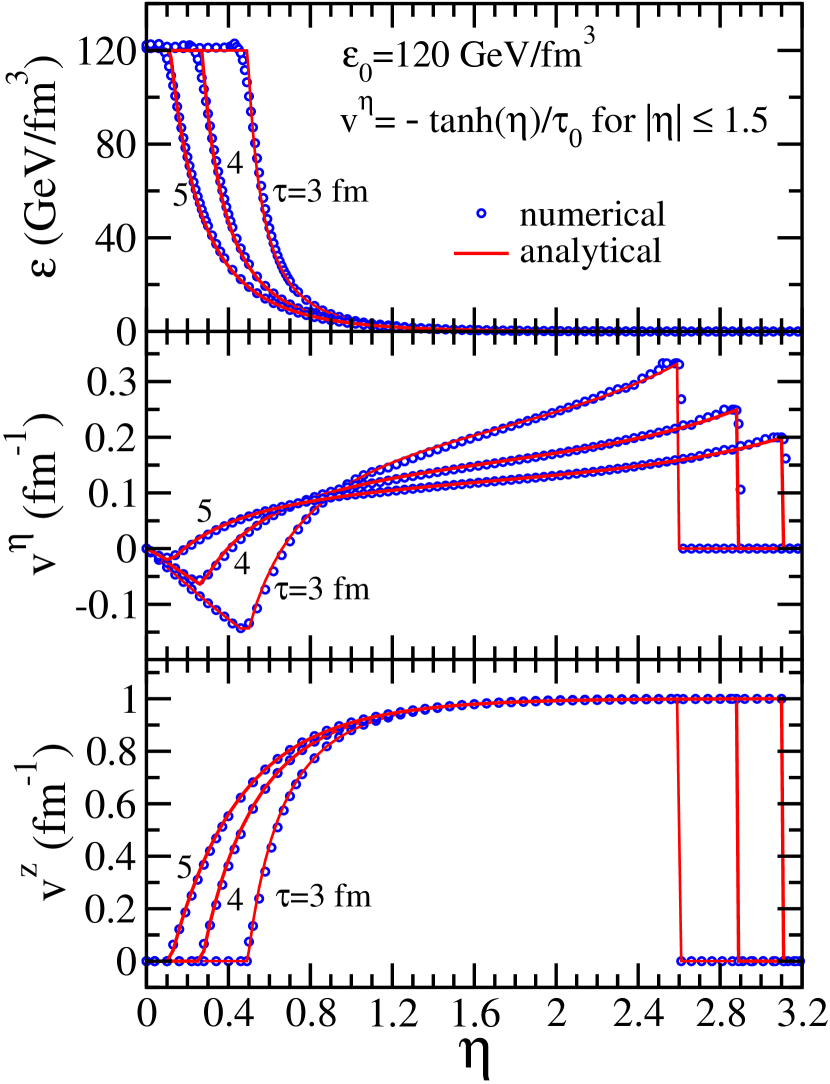
Figure 1: Comparison between the Riemann analytical solutions (lines) and the numerical results (circles) for the rapidity dependence of energy density $\epsilon$, velocities $v^{\eta}$ and $v^{z}$ at proper times $\tau=3,4,5$ fm/c for the initial condition of Eq. (III.1) at time $\tau_{0}=1$ fm/c.

Figure 1 shows comparison of numerical and analytic results, for the rapidity dependence of the energy density, velocity $v^{\eta}$, and the velocity $v^{z}$ obtained from Eq. (61) by using the corresponding $v^{\eta}$ values. All the results are at later times of $\tau=3,4,5$ fm/c. As the slab is at rest ($v^{z}=0$) in the Cartesian coordinate, which corresponds to $v^{\eta}<0$ in Milne coordinates. For $\eta>0$, a rarefaction wave starts at the edge of the slab (i.e at the discontinuity) and propagates within the slab with a velocity $c_{s}$. Also a shock starts at the discontinuity and moves into the vacuum with the speed of light. Such features are also observed at $\eta<0$ (not shown here). For instance at $\tau=3$ fm/c, we find $v^{z}=0$ for $|\eta|\leq 0.5$ and thus $v^{\eta}<0$. The rarefaction wave has then spread outside the slab from $0.5<|\eta|<2.6$, where $|\eta|=2.6$ correspond to the boundary of the vacuum. The fluid expands outward with increasing velocity $v^{\eta}$ till it reaches the boundary of the vacuum. The wave velocity $v^{z}$ rapidly increases outward and approaches the speed of light $v_{z}/c\approx 1$ at the vacuum. We find that our numerical results are in perfect agreement with the Riemann simple wave solution for all rapidity $\eta$ and all proper times $\tau$.

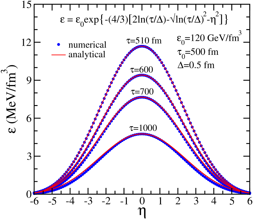
Figure 2: Comparison between the analytical solutions (lines) and the numerical results (circles) for the rapidity dependence of energy density $\epsilon$ at proper times $\tau=510,600,700,1000$ fm/c for the initial condition of Eq. (64) at time $\tau_{0}=500$ fm/c.

With increasing time, the two rarefaction waves, traversing inwards from positive and negative rapidity sides of the slab, will eventually reach the center $\eta=0$ of the slab and overlap. In practice, from this time onwards, Riemann solution cannot be applied, and the Landau-Khalatnikov solutions starts to be applicable. The Landau-Khalatnikov solution at the later times describe evolution of matter in the overlap region of the slab. At the asymptotic times $\tau\gg\Delta$, the Landau-Khalatnikov solution can be expressed as

$$\epsilon=\epsilon_{0}\left[-\frac{4}{3}\left\{2\ln\left(\frac{\tau}{\Delta}\right)-\sqrt{\ln\left(\frac{\tau}{\Delta}\right)^{2}-\eta^{2}}\right\}\right],$$ (64)

with $v^{\eta}=0$. Here $\Delta$ is the thickness of the slab where the two ingoing rarefaction waves overlap.

In the numerical simulation, the initial energy distribution are obtained from Eq. (64) corresponding to initial values of time $\tau_{0}=500$ fm/c, energy density $\epsilon_{0}=120$ GeV/fm³ and slab thickness $\Delta=0.5$ fm. Figure 2 shows the comparison between numerical results and the Landau-Khalatnikov asymptotic solution. The calculations are in good agreement with the analytical results up to large times especially around central rapidity region. At large rapidity the deviations from the asymptotic value may suggest that the rarefaction (overlapping) wave is mostly confined around the center region thus making the Landau-Khalatnikov asymptotic results invalid at large $|\eta|$.

III.2 Initial conditions for non-boost-invariant expansion

The initial conditions for our (1+1)D non-boost-invariant expansion of the viscous fluid at the initial proper time $\tau_{0}$ is defined by the three quantities, viz. $\epsilon(\tau_{0},\eta)$, $v_{\eta}(\tau_{0},\eta)$, $\pi^{xx}(\tau_{0},\eta)$. In our simulation we have adopted $\tau_{0}=0.4$ fm/c at which the initial energy density is taken as Schenke:2011bn

$$\epsilon(\tau_{0},\eta)=\epsilon_{0}\exp\left[-\frac{\left(|\eta|-\Delta\eta\right)^{2}}{2\sigma_{\eta}^{2}}\theta\left(|\eta|-\Delta\eta\right)\right].$$ (65)

This profile consists of a flat distribution about midrapidity of width $2\Delta\eta$ and two-smoothly connected Gaussian tails of half-width $\sigma_{\eta}$. The parameters $\epsilon_{0}$ and ($\Delta\eta,\sigma_{\eta}$) are adjusted to reproduce the absolute magnitude and width of the final rapidity distribution of mesons measured by BRAHMS Bearden:2004yx in central Au+Au collisions at the RHIC energy of $\sqrt{s_{NN}}=200$ GeV. The initial values of the longitudinal velocity profile is taken as boost-invariant, and the viscous stress tensor as isotropic:

$$v_{\eta}(\tau_{0},\eta)=0,~{}~{}~{}~{}\pi^{mn}(\tau_{0},\eta)=0.$$ (66)

The hydrodynamic evolution is continued until each fluid cell reaches a decoupling temperature of $T_{\rm dec}=150$ MeV. We consider only direct pion and kaon production and do not include their formation from resonance decays. To account for the latter contribution, we follow the prescription of Bozek:2007qt by noting that, since $\sim 75\%$ of pions originate from resonance decays Torrieri:2004zz , the rapidity distribution of Eq. (II.4) is multiplied by a factor of four.

The equation of state (EoS) influences the longitudinal expansion of the fluid and the two-particle correlations. In this work, the effects of EoS on the correlators have studied by employing both a conformal QGP fluid with the thermodynamic pressure $p=\epsilon/3$, and the s95p-PCE EoS Huovinen:2009yb which is obtained from fits to lattice data for crossover transition and matches to a realistic hadron resonance gas model at low temperatures $T$, with partial chemical equilibrium (PCE) of the hadrons at temperatures below $T_{\rm PCE}\approx 165$ MeV. Unless otherwise mentioned, the shear relaxation time in Eqs. (II.1) and (4) is set at $\tau_{\pi}=5\eta_{v}/4p$ corresponding to $\tau_{\pi}=5\eta_{v}/(sT)$ in the conformal fluid.

Table 1: The parameters of the initial energy distribution $\epsilon_{0},\sigma_{\eta}$ with $\Delta\eta=0.6$ corresponding to Eq. (65), that reproduce the final pion rapidity distribution in $0-5\%$ central Au+Au collisions at $\sqrt{s_{NN}}=200$ GeV. The results are in ideal and viscous hydrodynamic evolution in the MIS theory with EoS for conformal fluid, and that for lattice EoS are shown in braces. The last column gives the lifetime of the fluid at a freeze-out temperature of $T_{\rm dec}=150$ MeV.

$\eta_{v}/s$		$\epsilon_{0}$ (GeV/fm3)		$\sigma_{\eta}$		$\tau_{f}$ (fm/c)
0		200 (39.0)		0.9		16.40 (15.84)
0.08		142 (27.1)		1.0		16.08 (15.36)
0.24		82 (17.5)		1.4		14.88 (14.16)

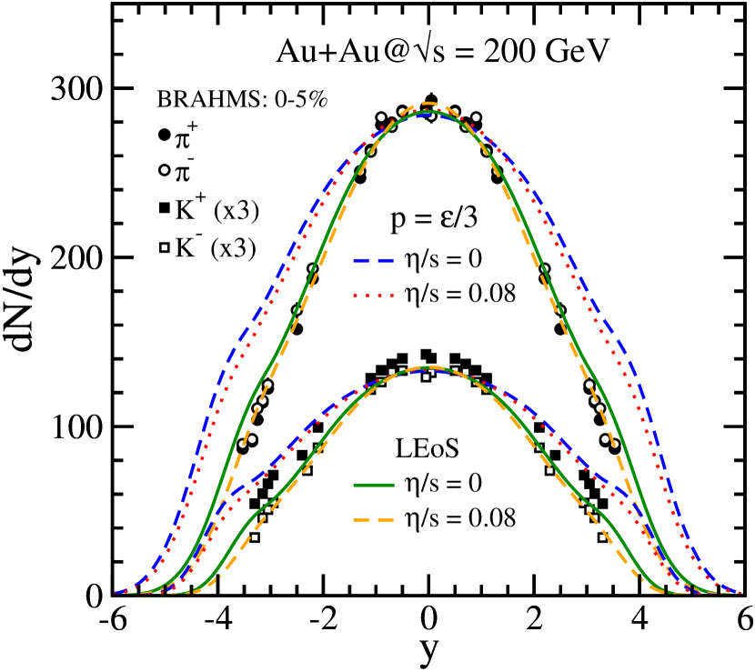
Figure 3: Rapidity distribution of $\pi^{\pm}$ and $K^{\pm}$ in $0-5\%$ central Au+Au collisions at $\sqrt{s_{NN}}=200$ GeV. The symbols represent the BRAHMS data Bearden:2004yx , and the lines correspond to non-boost-invariant hydrodynamic calculations for the conformal fluid and lattice equation of state at the shear viscosity to entropy density ratio of $\eta_{v}/s=0$ and 0.08 in the MIS approach.

Figure 3 shows the rapidity distribution of pions and kaons in our (1+1)D non-boost-invariant hydrodynamic model as compared with the $5\%$ most central Au+Au collision data from BRAHMS Bearden:2004yx . The parameters ($\epsilon_{0},\Delta\eta,\sigma_{\eta}$) obtained by fitting the data for pions at midrapidity are listed in Table I. The stiff conformal EoS induces an accelerated longitudinal flow with a much wider dN/dy as compared to the data. In fact, this EoS fails to reproduce the data at large rapidities for any combination of the parameters (or with varying $T_{\rm dec}$). In contrast, the softening produced due to deconfinement transition in the lattice EoS gives a smaller longitudinal pressure gradients and leads to a better agreement with rapidity distributions. As compared to ideal-hydrodynamics, the second-order viscous hydrodynamics slows down the expansion of the fluid, and thus requires a smaller and wider initial energy density distribution (see Table I) to be compatible with the final meson rapidity distribution.

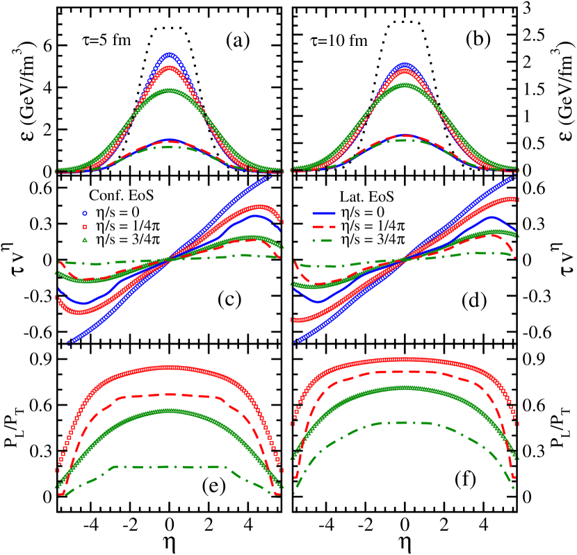
Figure 4: Space-time rapidity dependence of (a)-(b) energy density, (c)-(d) longitudinal velocity (scaled by time), and (e)-(f) longitudinal to transverse pressure ratio $P_{L}/P_{T}$, in the hydrodynamic calculations at proper times of $\tau=5$ fm (left panels) and 10 fm (right panels). The results are for ultra-relativistic gas (symbols) and lattice (lines) equations of state with $\eta_{v}/s=0,1/4\pi,3/4\pi$ in the MIS theory. The black dotted line is the Bjorken scaling solution $\epsilon/\epsilon_{0}\sim(\tau_{0}/\tau)^{4/3}$.

In Fig. 4 we present the space-time rapidity dependence of energy density $\epsilon$, longitudinal flow velocity $v_{\eta}$, and the ratio of longitudinal and transverse pressure, $P_{L}/P_{T}=(p_{0}-\pi_{0}/2)/(p_{0}+\pi_{0}/2)$ at the proper times of $\tau=5$ and 10 fm obtained in our non-boost-invariant model. The energy density in the perfect-fluid conformal hydrodynamics (blue circles in Fig. 4(a)-(b)) shows a decreasing flat region at midrapidity with increasing time as compared to initial profile. In contrast to boost-invariant expansion, the stronger longitudinal expansion due to larger pressure gradients in the non-boost-invariant case transfer energy faster to larger rapidities. Indeed, in the Bjorken scaling solution for a perfect-fluid, the energy density $\epsilon(\tau)=\epsilon(\tau_{0})(\tau_{0}/\tau)^{4/3}$ (black dotted line) is seen to lie above (below) than that in the (1+1)D case at midrapidity (large rapidities). Thus, in general, a Bjorken expansion would underestimate the cooling of the system. The discrepancies become larger with time as can be seen in Fig. 4(b) at $\tau=10$ fm/c. The inclusion of viscosity slows down the expansion and thereby the cooling of the system. As a result, the energy density distribution for $\eta_{v}/s=0.08$ (red squares) and $\eta_{v}/s=0.24$ (green triangles) for the ultra-relativistic gas becomes increasingly comparable to the perfect fluid case, inspite of smaller initial energy values in the dissipative hydrodynamics (see Table I). For the softer lattice EoS, the differences in the energy densities for various $\eta_{v}/s$ (lines in Fig. 4(a)-(b)) become increasingly smaller with increasing $\tau>\tau_{0}$.

Figure 4(c)-(d) shows that the longitudinal flow velocity $v_{\eta}$ distribution (multiplied by the corresponding proper time) rapidly increases with rapidity in the ideal-fluid dynamics. Although we initialized the fluid with a boost-invariance value at all rapidities, i.e. $v_{\eta}(\eta,\tau_{0})=0$, the longitudinal pressure gradients quickly accelerate the fluid and breaks the longitudinal boost-invariance at $\tau>\tau_{0}$. In our second-order viscous evolution, viscosity restricts the pressure gradients and reduces the increase of $v_{\eta}$ with $\eta$. At large rapidities, the smaller pressure (and temperature) enhances the time $\tau_{\pi}=5\eta_{v}/4p$ for the system to relax towards equilibrium. As a consequence, the larger viscous corrections here decelerates the expansion and eventually overcomes the acceleration from pressure gradients. This causes $v_{\eta}$ to approach the Bjorken limit, and beyond this rapidity the second-order viscous hydrodynamics becomes questionable. With increased $\eta_{v}/s=0.2$, the stronger viscous effects drive the system toward this unphysical behavior at an earlier rapidity. As the longitudinal flow velocity build-up with increasing evolution time, at the later time of $\tau=10$ fm/c, its appearance is delayed to larger rapidity value (see Fig. 4). Compared to the stiff EoS, $p=\epsilon/3$, the lattice EoS injects a smaller pressure gradient resulting in a smaller deviation from the Bjorken flow profile, especially at large $\eta_{v}/s$.

The pressure anisotropy $P_{L}/P_{T}$ (4(e)-(d)) shows marked deviation from the isotropic initial pressure configuration of $P_{L}/P_{T}=1$. As the shear stress tensor $\pi^{\eta\eta}$ gradually build-up with time and later decreases slightly, the anisotropy is larger at $\tau=5$ fm/c than at 10 fm/c. At large rapidities, $\pi^{\eta\eta}$ becomes comparable to the thermodynamic pressure, hence $P_{L}/P_{T}$ rapidly decreases and can eventually become negative. Although an increase in $\eta_{v}/s$ leads to a smaller $P_{L}/P_{T}$ at midrapidity, a somewhat wider initial energy distribution (see Table I) prevents an early appearance of this unphysical region at any given time. As expected, the dissipative effects are more pronounced in the lattice EoS and results in larger pressure anisotropy.

The large space-time variation of the flow and pressure anisotropy, as found here in a finite fluid system, should have important effects on the two-particle rapidity correlations arising from the propagation of thermal noise.

III.3 Single thermal fluctuation on top of (1+1)D viscous expanding medium

For a clear understanding of the evolution of hydrodynamic fluctuations and the resulting rapidity correlations induced by thermal fluctuations at all space-times, it is instructive to focus first on the evolution of one static thermal perturbation. In particular, we consider a static Gaussian thermal fluctuation induced at ($\eta_{0},\tau_{0}$) on top of non-boost-invariant expanding medium:

$$\delta T(\eta,\tau_{0})= ~{}T(\eta_{0},\tau_{0})\frac{\kappa}{(2\pi\sigma)^{1/2}}{\rm exp}\left[-(\eta-\eta_{0})^{2}/2\sigma^{2}\right],$$

$$\delta u^{\eta}(\eta,\tau_{0})= ~{}\delta\pi^{\eta\eta}(\eta,\tau_{0})=0.$$ (67)

At the initial time $\tau_{0}=0.4$ fm/c, the perturbation is induced at the fluid rapidity $\eta_{0}$ and has a Gaussian width parameter $\sigma=0.2$ and amplitude $\kappa=0.1\sqrt{2\pi\sigma}$.

The perturbation travels in opposite directions such that in the local rest frame of the background fluid, the speed of propagation is the sound velocity $c_{s}=\pm(dz/dt)_{\mathrm{LRF}}$. Writing this covariantly one obtains $u_{0}^{\mu}\varepsilon_{\mu\alpha}dx^{\alpha}=\pm c_{s}u_{0\mu}dx^{\mu}$, where $\varepsilon^{\mu\nu}$ is the totally antisymmetric tensor of rank 2. Noting that in $(\tau,\eta)$ coordinates $\varepsilon_{\tau\eta}=\tau$, the equation of motion of the perturbation peak is found to be,

$$\tau\frac{d\eta}{d\tau}=\frac{\pm c_{s}+\tau v_{\eta_{0}}}{1\pm c_{s}\tau v_{\eta_{0}}}$$ (68)

In case of Bjorken expansion where $v_{\eta_{0}}=0$, the above expression has the simple solution $\eta=\eta_{0}\pm c_{s}\log(\tau/\tau_{0})$. For the (1+1)D expansion, Eq. (68) has to be integrated numerically as $v_{\eta_{0}}(\tau,\eta)$ is not known analytically. It is important to note that unlike the Bjorken case, where the extent of propagation of perturbations is independent of the dissipative equations considered, in the (1+1)D case the shear stress tensor controls the width of sound cone by determining the background flow profile $v_{\eta_{0}}$ seen in Fig. 4.

In addition to influencing the trajectories of perturbations, an expanding fluid also leads to diffusion of the propagating disturbance. For example, in an ideal fluid at rest, a perturbation would propagate unattenuated in opposite directions at the speed of sound, whereas, in a Bjorken expansion (even in the ideal limit) the disturbance broadens and dampens during propagation. This is attributed to the non-linear dispersion relation for wave propagation on top of Bjorken expansion, $\omega(k)=i(1-c_{s}^{2})/2\pm\sqrt{c_{s}^{2}k^{2}-(1-c_{s}^{2})^{2}/4}$. In the (1+1)D expansion, the dispersion relation becomes complicated via dependences on space-time and has to be obtained numerically. The propagation of temperature disturbance will induce perturbation in velocity $\delta u^{\eta}$ and shear pressure tensor $\delta\pi$ at later times $\tau>\tau_{0}$.

The rapidity distribution of the correlations induced by these fluctuations can be explored via the equal-time rapidity correlation,

$$C_{\Delta X,\Delta Y}(\tau,\Delta\eta;\eta_{0})=\int d\eta^{\prime}\Delta X(\eta^{\prime},\tau)\Delta Y(\eta^{\prime}+\Delta\eta,\tau),$$ (69)

where $\eta_{0}$ is the initial position of the disturbance at time $\tau_{0}$ and $(\Delta X,\Delta Y)$ refer to the the normalized fluctuations $\Delta T=\delta T(\eta,\tau)/T_{0}(\eta,\tau)$, $\Delta u^{\eta}=\tau\delta u^{\eta}$ and $\Delta\pi=\delta\pi/(\epsilon_{0}+p_{0})$. Due to explicit dependence of the background evolution on space-time rapidity $\eta$, the above correlator would depend on the initial $\eta_{0}$ where the perturbation is introduced. This is to be contrasted with the Bjorken expansion where the translational invariance (in $\eta$ direction) of the background flow implies that $C_{\Delta X,\Delta Y}$ does not depend on the initial rapidity position of the perturbation Shi:2014kta .

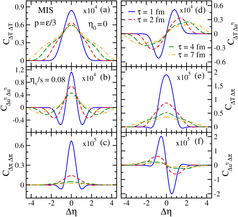
Figure 5: Equal-time longitudinal rapidity correlations $C_{\Delta X,\Delta Y}(\tau,\Delta\eta;\eta_{0})$ with $(\Delta X,\Delta Y)\equiv[\delta T/T_{0},\tau\delta u^{\eta},\delta\pi/(\epsilon_{0}+p_{0})]$ computed as a function of space-time rapidity separation $\Delta\eta$ at various later times from a thermal perturbation at an initial time of $\tau_{0}=0.4$ fm/c and at rapidity $\eta_{0}=0$. The perturbation is induced on top of non-boost-invariant background hydrodynamic flow in the MIS theory using an ultra-relativistic gas EoS with $\eta_{v}/s=1/4\pi$. The correlators in each panel are vertically scaled by a representative value.

In Fig. 5, we present rapidity correlations at later times arising due to a static initial thermal perturbation induced at the center $\eta_{0}=0$ of the background fluid undergoing (1+1)D hydrodynamic expansion in the MIS theory. We consider a $p=\epsilon/3$ EoS and $\eta_{v}/s=0.08$; the other initial and freeze-out conditions of the background are given in Table I. Figure 5(a) shows that at early times the temperature-temperature rapidity correlation $C_{\Delta T\Delta T}$ has a large and narrow peak at $\Delta\eta=0$ due to self-correlations. With the expansion of the background fluid, the amplitude of the peak decreases with time as it spreads over a large rapidity separation leading to long-range rapidity correlations till the freeze-out of the system is reached at $\tau_{f}\approx 16$ fm/c. The extent of the rapidity correlation at any given time is bounded by the maximum distance travelled by the sound wave, namely the sound horizon, which can be obtained by solving Eq. (68). In contrast, rapidity correlation from ripples on top of a boost-invariant ideal background fluid was shown Shi:2014kta to generate a sharp peak at $\Delta\eta\approx 0$, followed by a relatively flat region at intermediate $\Delta\eta$, and a much smaller peak from the sound horizon at large $\Delta\eta$. Thus, in the present (1+1)D viscous hydrodynamic expansion, the much broader rapidity correlation (with negligibly small second peak) that persists even at late times can be attributed to the interplay of nonzero background fluid velocity $v_{\eta_{0}}(\tau,\eta)$ and viscous damping in the MIS theory.

Figure 5(b) shows the time-evolution of velocity-velocity rapidity correlation $C_{\Delta u^{\eta}\Delta u^{\eta}}$. Starting with an initial value of $\delta u^{\eta}=0$, the velocity perturbations and correlations at first build-up with time at about zero rapidity separation and then decreases later when the perturbation spreads to large rapidities. The negative correlations seen at larger rapidity separations are essentially due to $\delta u^{\eta}$ having opposite signs along positive and negative directions relative to the initial position of perturbation. Careful examination of Figs. 5(a), (b) shows that the minima in this negative correlations are produced at the sound horizon corresponding to the “second peak” in the temperature-temperature correlation.

The pressure-pressure rapidity correlation due to shear $C_{\Delta\pi\Delta\pi}$ shown in Fig. 5(c), exhibits a similar peaked structure as seen for temperature-temperature correlations. However, the magnitude of this correlation is much smaller and does not spread much in rapidity separation with increasing time. Note that in the present initialization of temperature perturbation (instead of velocity or shear-pressure perturbations), the magnitude of $C_{\Delta T\Delta T}$ dominates and it is about two orders of magnitude larger than $C_{\Delta u^{\eta}\Delta u^{\eta}}$.

On the other hand, the rapidity correlations $C_{\Delta T\Delta u^{\eta}}$ and $C_{\Delta u^{\eta}\Delta\pi}$ [see Figs. 5(d), (f)] are odd functions of $\Delta\eta$ and thus the correlations vanish at $\Delta\eta=0$. Moreover, the “cross” correlations follow $C_{\Delta X,\Delta Y}=-C_{\Delta X,\Delta Y}$. The structure of the $C_{\Delta T\Delta\pi}$ correlator in Fig. 5(e) can be easily understood from the $C_{\Delta T\Delta T}$ and $C_{\Delta\pi\Delta\pi}$ correlations.

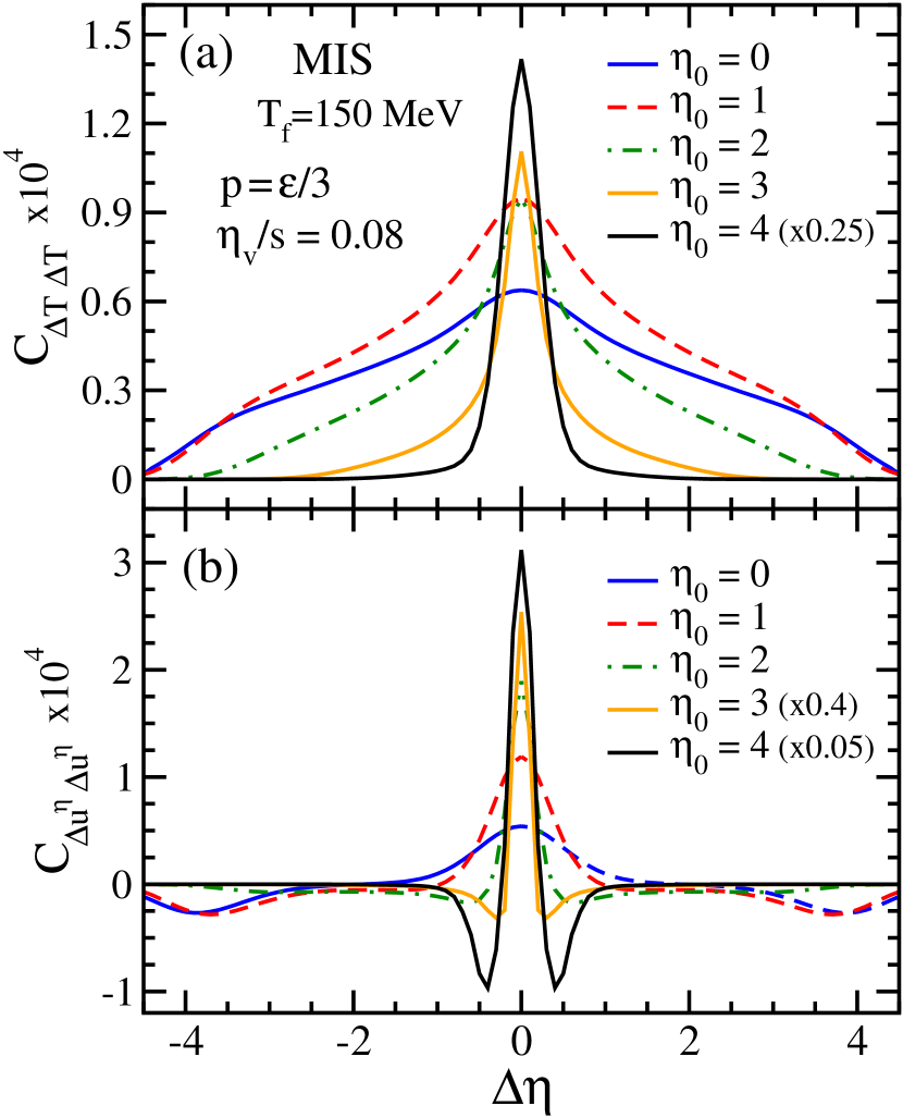
Figure 6: Temperature-temperature and velocity-velocity rapidity correlations as a function of rapidity separation $\Delta\eta$ arising from perturbations at various initial rapidities $\eta_{0}$ and computed at a freeze-out hypersurface $T_{\rm dec}=150$ MeV. The perturbations are induced on top of non-boost-invariant background hydrodynamic flow in the MIS theory for an ultra-relativistic gas EoS with $\eta_{v}/s=1/4\pi$. The correlators for large $\eta_{0}$ are scaled vertically by the values shown within braces.

In Figs. 6(a), (b) we show the correlations between temperature-temperature and velocity-velocity at the freeze-out hypersurface $T(\tau_{f},\eta)=T_{\mathrm{dec}}$, induced by a single temperature perturbation placed at various initial rapidity values $\eta_{0}$. Accordingly, we now use the definition of the correlator $C_{\Delta X,\Delta Y}(T_{\mathrm{dec}},\Delta\eta;\eta_{0})=\int d\eta^{\prime}\Delta X(\eta^{\prime},T_{\mathrm{dec}})\Delta Y(\eta^{\prime}+\Delta\eta,T_{\mathrm{dec}})$. For perturbation introduced at a large rapidity, we find the self-correlations to increase and the long-range correlations to decrease. This is because the fluid cells at large rapidities (having small initial temperatures) freeze-out at early times Florkowski:2016kjj and thus one of the perturbation peaks which propagates along the background flow reaches the freeze-out hypersurface quickly and is effectively undamped. Consequently, the self-correlations which are essentially squares of the peak values, increase with $\eta_{0}$ of the initial perturbation. However, the long-range correlation which depends on the product of the two peaks decrease as the other peak which travels opposite to the background fluid takes substantially longer to reach the freeze-out surface and is almost fully damped; see Fig. 6(a). As seen in Fig. 6(b), the rise in self-correlations with $\eta_{0}$ is found to be more for the velocity-velocity correlator due to the pronounced background acceleration of the fluid at large $\eta$, which leads to build up of the velocity of the travelling perturbation.

III.4 Thermal noise correlations on top of (1+1)D viscous expanding medium

In this section, we shall explore longitudinal rapidity correlations induced by thermal fluctuations in the non-boost-invariant (1+1)D expansion of the background medium. These fluctuations, which act as source terms for linearized hydrodynamic equations are correlated over short length-scales, and accordingly they generate singularities in the correlators for hydrodynamic variables at zero rapidity separation and at the sound horizons. While for Bjorken expansion within the Navier-Stokes theory, the correlators can be analytically decomposed into regular and singular parts Chattopadhyay:2017rgh , in the second-order MIS and CE theories such analytic separation is not plausible. In Eq. (II.4) for the two-particle rapidity correlations calculated at freeze-out, the singularities get smeared out by the coefficients ${\cal F}_{X}$ [with $X\equiv(T_{1},u_{1}^{\eta},\pi_{1})$], thereby allowing for a smooth presentation. In order to explore at various times $\tau\leq\tau_{f}$, the equal-time longitudinal rapidity correlation arising from thermal noise, we consider a Gaussian convoluted correlation

$$\langle C_{X,Y}(\Delta\eta,\eta;\tau)\rangle= \int d(\Delta\eta^{\prime})\langle X(\eta,\tau)Y(\eta+\Delta\eta^{\prime},\tau)\rangle$$

$$\times{\rm exp}\left[-(\Delta\eta-\Delta\eta^{\prime})^{2}/2\sigma_{\small\Delta\eta}^{2}\right],$$ (70)

where $(X,Y)\equiv(\delta T,\delta u^{\eta},\delta\pi)$ refer to the usual perturbations in the event. An averaging $\langle\cdots\rangle$ has been performed over many fluctuating events that evolve on top of background hydrodynamics; the initial conditions for the latter is given in Table I. Note that although the qualitative nature of the correlations are insensitive to the smearing function, whose width we have taken as $\sigma_{\Delta\eta}=0.4$, the the magnitude and spread of the peaks depend on the latter.

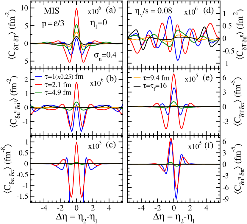
Figure 7: Event averaged equal-time longitudinal rapidity correlations $\langle C_{X,Y}(\Delta\eta,\eta)\rangle$ with $(X,Y)\equiv(\delta T,\delta u^{\eta},\delta\pi)$ computed as a function of space-time rapidity separation $\Delta\eta=\eta_{1}-\eta_{2}$ about $\eta_{1}=0$ at various times due to thermal noise perturbations on top of non-boost-invariant background flow. The results are in the Müller-Israel-Stewart (MIS) theory for ultra-relativistic gas EoS with $\eta_{v}/s=1/4\pi$. The correlators in each panel are scaled vertically by values given; the correlations at $\tau=1$ fm/c are further scaled by 0.25 for clarity.

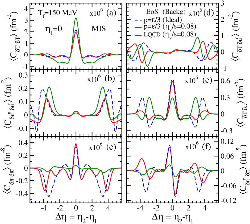
Figure 8: Event averaged rapidity correlations $\langle C_{X,Y}(\Delta\eta,\eta)\rangle$ with $(X,Y)\equiv(\delta T,\delta u^{\eta},\delta\pi)$ at midrapidity from thermal noise at the freeze-out temperature $T_{\rm dec}=150$ MeV. The results are in the MIS formalism with $\eta_{v}/s=1/4\pi$ in the average and thermal noise evolution for $p=\epsilon/3$ EoS (red solid line), lattice EoS (green solid line) and an ideal background evolution with $p=\epsilon/3$ EoS (blue dashed line). The initial and final conditions for the background evolution are given in Table I. All the correlations are scaled vertically by $10^{6}$.

Figure 7 displays equal-time rapidity correlations for various fluctuations arising from thermal noise on top of (1+1)D hydrodynamic expansion in the MIS theory with $\eta_{v}/s=0.08$ in both the background and noise evolution equations. Thermal fluctuations at each spatial point and during the entire evolution of the fluid produce short-range temperature-temperature correlation peaked at zero rapidity separation, see Fig. 7(a). In contrast to correlation from an initial perturbation [see Fig. 5(a)], a much narrower peak is seen in thermal noise. The appreciable negative correlations at small rapidity separation is due to the second-derivative of the delta function arising from the noise term in momentum conservation equation. In fact, the magnitude of the peaks and troughs are dominated by the singularities that occur at $\Delta\eta=0$ due to self-correlations and at sound horizons. This lead to non-monotonous structures in the correlations induced by thermal noise at large $\Delta\eta$ in contrast to that seen from a single perturbation. At later times, the expansion of the fluid causes the peak values to decrease and the correlations to spread somewhat farther in rapidity separations.

The velocity-velocity and shear pressure-pressure rapidity correlations shown in Figs. 7(b), (c) also give pronounced negative correlations from the singularities at small $\Delta\eta$. While the $\langle C_{\delta u^{\eta},\delta u^{\eta}}\rangle$ correlation give nontrivial structures about the sound horizon, the $\langle C_{\delta\pi,\delta\pi}\rangle$ correlation essentially has a small magnitude and rapidly damp at larger $\Delta\eta$. Consequently, the cross correlations $\langle C_{\delta T,\delta\pi}\rangle$ and $\langle C_{\delta u^{\eta},\delta\pi}\rangle$ have negligible values at large rapidities and contribute minimally to the final two-particle rapidity correlations. By inspection of Figs. 5 and 7 it is clearly evident that compared to an induced perturbation, the realistic hydrodynamic fluctuations in (1+1)D expansion generate rich structures at short and long range two-particle rapidity correlations.

To gauge the importance of underlying flow and viscous damping, we compare in Fig. 8 the rapidity correlations $\langle C_{X,Y}(\Delta\eta,\eta)\rangle$ at the freeze-out hypersurface corresponding to $T_{\rm dec}=150$ MeV in the MIS theory at $\eta_{v}/s=1/4\pi$ (red solid lines) and also for ideal background hydrodynamic evolution (blue dashed line) for ultra-relativistic gas EoS. In absence of viscous damping larger peaks and troughs can be seen at small $\Delta\eta$. Moreover, the fluctuations travel over large rapidity separation and generate distinct structures about the sound horizon. We also present correlations computed for a lattice EoS in the MIS theory at $\eta_{v}/s=1/4\pi$ (green solid lines). The smaller sound velocity near the deconfinement transition slows down the expansion of the background fluid (see Fig. 4) as well as limits the spatial extent of the sound horizon. These lead to sharp peaks from self-correlation and large and broad negative correlations from the singularities at $\Delta\eta\approx 0$ and sound horizon. In fact, the total correlation in the lattice is dominated by the temperature-temperature correlations.

III.5 Two-particle rapidity correlations in (1+1)D expanding medium

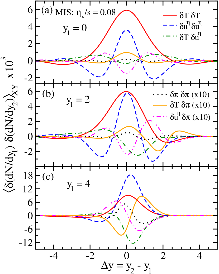
Figure 9: Two-particle rapidity correlations for different fluctuations calculated for charged pions as a function of pion-rapidity separation $\Delta y=y_{1}-y_{2}$ at rapidities $y_{1}=0,2,4$ in the MIS hydrodynamics. The results are for ideal gas EoS with $\eta_{v}/s=1/4\pi$ and the initial and final conditions are the same as in Fig. 7.

In this section we will study the effects of thermal fluctuations on two-particle rapidity correlations for charged pions in expanding non-boost-invariant background fluid. As discussed above, the singularities in the two-point correlators $\langle X(\eta_{1})Y(\eta_{2})\rangle$ (with $X,Y\equiv\delta T,\delta u^{\eta},\delta\pi$) of Eq. (II.4) are smeared out by the function ${\cal F}_{X,Y}$ leading to clear observable structures in the computed correlations at freeze-out. In Fig. 9 we present the various rapidity correlators $\langle(\delta dN/dy_{1})(\delta dN/dy_{2})\rangle_{X,Y}$ for charged pions as a function of kinematic rapidity separation $\Delta y=y_{1}-y_{2}$ in the MIS theory with $\eta_{v}/s=0.08$ in the average and noise parts of the evolution equations. The correlators get broadened when these are convoluted with the smearing functions ${\cal F}_{\delta T}$ (which is roughly Gaussian about $\Delta\eta=0$) and ${\cal F}_{\delta u^{\eta}}$ (which has peaks at $\Delta\eta\approx 1.5$ and vanishes at $\Delta\eta=0$).

As also evident from Fig. 8, the two-pion rapidity correlations about midrapidity $y_{1}=0$ of a pion (see Fig. 9(a)) is dominated by temperature-temperature correlation at $\Delta y=0$. At $\Delta y\gtrsim 2$ the distinct rapidity dependent structures in the correlations $\delta T\delta T$, $\delta u^{\eta}\delta u^{\eta}$ and their cross correlations contribute almost equally to the long-range rapidity correlations. The correlations associated with the shear stress tensor $\delta\pi$ are found quite small at all rapidity separations.

At large pion rapidity $y_{1}>0$, inspite of smaller magnitude of initial energy densities and hence reduced strength of noise source as evident from Eq. (II.3), the enhanced longitudinal velocity gradients induce larger fluctuations especially for the velocity correlations. Figures 9(b), (c) show that with increasing pion rapidity, the correlations involving $\delta u^{\eta}$ and $\delta\pi$ become increasingly important. However, the correlations here are short-ranged as the fluctuations produced at large $y_{1}$ reach the freeze-out hypersurface quickly without substantial spreading. Moreover, the negative correlations about $\Delta y\sim 0$ become appreciable so that the total contribution to the two-pion correlation would be smaller than at midrapidity.

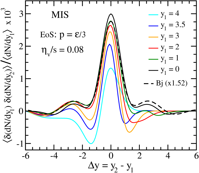
Figure 10: Correlation function of charged pions normalized with single-particle rapidity distribution in (1+1)D hydrodynamic expansion as a function of rapidity separation $\Delta y=y_{1}-y_{2}$ at various rapidities $y_{1}$. The results are in the MIS theory for ideal gas EoS with $\eta_{v}/s=1/4\pi$ and the initial and final conditions are the same as in Fig. 7. The corresponding correlation in the Bjorken expansion but normalized by $(dN/dy_{1})_{y_{1}=0}$ is shown by black dashed line.

In Fig. 10 we present the two-particle rapidity correlation for charged pions at various rapidities $y_{1}$ in the MIS viscous evolution for an ultra-relativistic gas EoS with $\eta_{v}/s=1/4\pi$ in both the noise and background evolution. This has been computed by summing the various components of the noise correlations as in Eq. (II.4) and displayed in Fig. 9. For the (1+1)D viscous expansion, the correlations at small rapidities $y_{1}$ produce pronounced short-range peaks and interesting structures at large rapidity separation. On the other hand, for larger pion rapidities $y_{1}$ the correlations result in smaller peaks at $\Delta y$ and are largely asymmetric about midrapidity. Furthermore, the singularities mainly from self-correlation at $\Delta y$ are found to be substantial.

We also show the corresponding correlations for boost-invariant expansion (Bjorken flow) in the MIS theory computed with the same initial time and constant initial energy density as given in Table I at $T_{\rm dec}=150$ MeV. For equivalent comparison the correlation in the Bjorken case is normalized by the rapidity density $(dN/dy_{1})_{y_{1}=0}$ for the non-boost-invariant expansion. Even after this scaling, the short-range correlation at mid-rapidity is found to be slightly larger for the (1+1)D case due to more contribution from self-correlations on the freeze-out hypersurface.

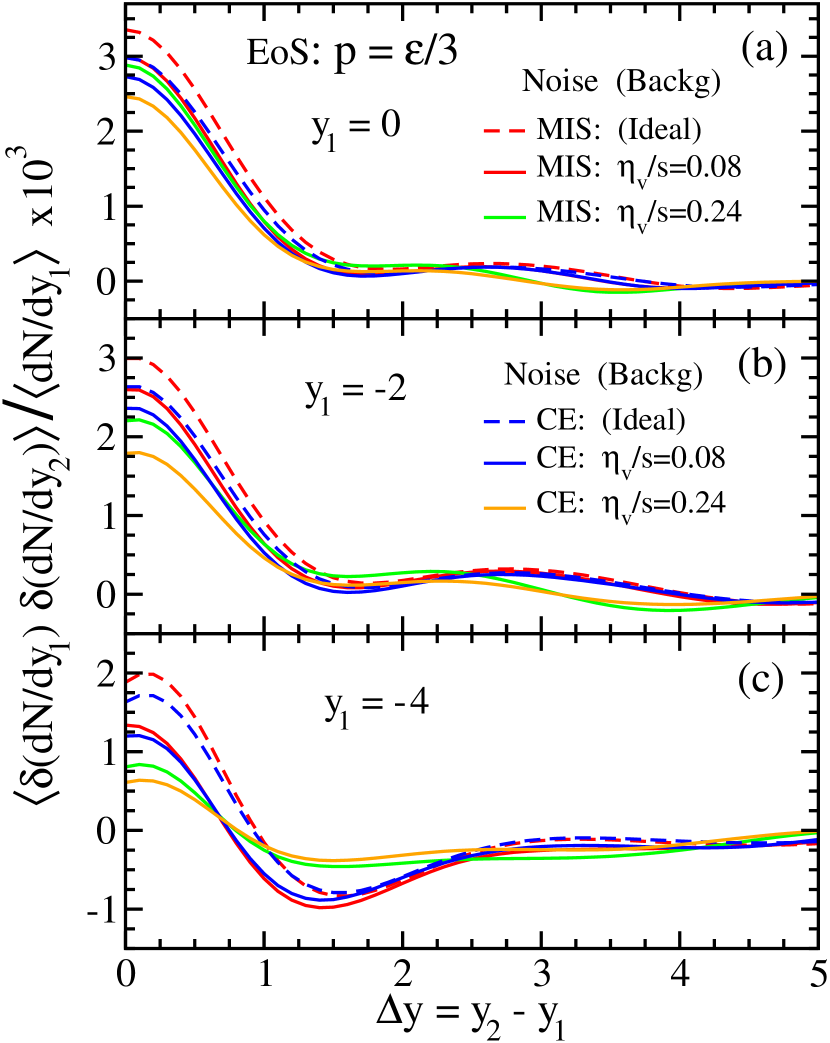
Figure 11: Correlation function of charged pions normalized with single-particle rapidity distribution as a function of rapidity separation $\Delta y=y_{1}-y_{2}$ at various rapidities $y_{1}$. The results are in the Müller-Israel-Stewart (MIS) and Chapman-Enskog (CE) formalisms for thermal noise evolution and compared with the ideal background hydrodynamic evolution. An ideal gas EoS ($p=\epsilon/3$) is used and the the initial and freeze-out conditions are given in Table I.

Figure 11(a)-(c) compares the two-particle rapidity correlation for charged pions in the Müller-Israel-Stewart (MIS) and Chapman-Enskog (CE) dissipative evolutions for an ultra-relativistic gas EoS. Using ideal hydrodynamics for the background evolution and MIS (red dashed line) and CE (blue dashed line) theories for the evolution of thermal noise with $\eta_{v}/s=0.08$, we find that for all pion rapidities $y_{1}$, the short-range correlation peak at $\Delta y\approx 0$ has a larger magnitude in MIS than in CE. This arises due to the smaller damping coefficient $\lambda_{\pi}$ in MIS Eq. (29) leading to larger fluctuations as also evident from Fig. 8 for the noise correlators at freeze-out. At larger $\Delta y$, the singularities in the correlators are more prominent only for large pion rapidities $|y_{1}|\sim 4$ resulting in somewhat clear separation of the structures in MIS and CE formalisms.

On inclusion of viscosity in the background evolution (solid lines), the correlation strengths at $\Delta y$ are suppressed due to viscous damping at small rapidities $y_{1}$. However, the long-range structures at large rapidity-separation are rather insensitive to viscosity in both the MIS and CE theories. Note that the initial energy densities have been readjusted to reproduce the charged hadron rapidity distribution as given in Table I. It is important to note that compared to the Bjorken evolution Chattopadhyay:2017rgh , in the present non-boost-invariant dynamics the fluctuations cause somewhat smaller short-range correlation peak ($\Delta y\sim 0$) at larger values of particle rapidity $y_{1}$. A larger $\eta_{v}/s=0.24$ in the fluctuation evolution leads to further damping of the correlations due to smearing of the peaks associated with sound horizon.

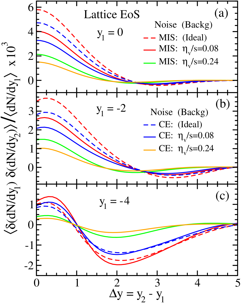
Figure 12: Similar to Fig. 11 but with a lattice EoS. The initial and freeze-out conditions are given in Table I.

In Fig. 12 we compare the two-particle rapidity correlations for charged pions in the MIS and CE viscous evolutions but for a lattice QCD EoS. We recall from Table I that the freeze-out time is somewhat smaller compared to that in the conformal EoS. Considerably enhanced two-pion correlation is found at about $\Delta y\sim 0$ for the lattice QCD EoS as compared to ideal gas EoS, with and without viscosity in the background evolution. This is primarily due to smaller velocity of sound in the medium with a lattice EoS that slows down the propagation of fluctuation over large separations. Here the effects of viscous damping on the rapidity correlations is found to be quite significant.

IV Summary and Conclusions

We have studied the evolution of thermal noise on top of a non-boost invariant medium expansion within the linearized hydrodynamic framework in both MIS and CE dissipative formalisms. The (1+1)D equations for the background (averaged) were solved using a newly developed code based on the SHASTA-FCT algorithm. Using a MacCormack type method to solve the linearized perturbation equations, we first studied the correlations induced by a single local disturbance propagating on top of the background medium, and then computed two-particle rapidity correlations induced by thermal fluctuations which are essentially disturbances (sources) that persist throughout hydrodynamic expansion. For a single perturbation introduced at some space-time rapidity $\eta_{0}$, the self-correlations induced on the $T_{\mathrm{d}ec}$ hypersurface were shown to increase with $\eta_{0}$, with the velocity-velocity correlator showing the maximum growth due to the background acceleration. Our results for the two-particle correlations show that unlike in the Bjorken scenario where correlations depend only on the rapidity separation $\Delta y$, for the (1+1)D expansion these structures strongly depend on the rapidity $y$ of the final state particle. Although at $y\sim 0$, the short-ranged structures ($\Delta y\sim 0$) are dominated by the temperature-temperature correlations, for large rapidities $y\geq 2$, the velocity-velocity correlations are responsible for the self-correlations. Inclusion of viscosity was found to reduce the auto-correlations in all the formalisms. For the lattice QCD EoS with smaller speed of sound, the correlations became larger at small $\Delta y\sim 0$ and long-range correlations get reduced, as compared to the ultra-relativistic EoS, due to a lesser extent of propagation of fluctuations in the former scenario.

References

- (1) J. Adams et al. [STAR Collaboration], Nucl. Phys. A 757, 102 (2005).
- (2) K. Adcox et al. [PHENIX Collaboration], Nucl. Phys. A 757, 184 (2005).
- (3) K. Aamodt et al. [ALICE Collaboration], Phys. Rev. Lett. 107, 032301 (2011).
- (4) G. Aad et al. [ATLAS Collaboration], Phys. Rev. C 86, 014907 (2012).
- (5) S. Chatrchyan et al. [CMS Collaboration], Phys. Rev. C 89, 044906 (2014).
- (6) P. Huovinen, P. F. Kolb, U. W. Heinz, P. V. Ruuskanen and S. A. Voloshin Phys. Lett. B 503, 58 (2001).
- (7) U. W. Heinz and P. F. Kolb, Nucl. Phys. A 702, 269 (2002).
- (8) I. Müller, Z. Phys. 198, 329 (1967).
- (9) W. Israel and J. M. Stewart, Annals Phys. (N.Y.) 118, 341 (1979).
- (10) A. Muronga, Phys. Rev. C 69, 034903 (2004).
- (11) P. Romatschke and U. Romatschke, Phys. Rev. Lett. 99, 172301 (2007).
- (12) A. Jaiswal, Phys. Rev. C 87, 051901 (2013).
- (13) R. S. Bhalerao, A. Jaiswal, S. Pal and V. Sreekanth, Phys. Rev. C 89, 054903 (2014).
- (14) C. Chattopadhyay, A. Jaiswal, S. Pal and R. Ryblewski, Phys. Rev. C 91, 024917 (2015).
- (15) M. Strickland, Nucl. Phys. A 926, 92 (2014).
- (16) U. W. Heinz, D. Bazow and M. Strickland, Nucl. Phys. A 931, 920 (2014).
- (17) M. Luzum and P. Romatschke, Phys. Rev. C 78, 034915 (2008) Erratum: [Phys. Rev. C 79, 039903 (2009)].
- (18) B. Schenke, S. Jeon and C. Gale, Phys. Rev. C 85, 024901 (2012).
- (19) Z. Qiu, C. Shen and U. Heinz, Phys. Lett. B 707, 151 (2012).
- (20) B. Alver and G. Roland, Phys. Rev. C 81, 054905 (2010) [Erratum-ibid. C 82, 039903 (2010)].
- (21) C. Gale, S. Jeon, B. Schenke, P. Tribedy and R. Venugopalan, Phys. Rev. Lett. 110, 012302 (2013).
- (22) R. S. Bhalerao, A. Jaiswal and S. Pal, Phys. Rev. C 92, 014903 (2015).
- (23) C. Chattopadhyay, R. S. Bhalerao, J. Y. Ollitrault and S. Pal, Phys. Rev. C 97, 034915 (2018).
- (24) P. Staig and E. Shuryak, Phys. Rev. C 84, 034908 (2011).
- (25) Y. Tachibana, N. B. Chang and G. Y. Qin, Phys. Rev. C 95, 044909 (2017)
- (26) J. I. Kapusta, B. Muller and M. Stephanov, Phys. Rev. C 85, 054906 (2012).
- (27) C. Young, Phys. Rev. C 89, 024913 (2014).
- (28) J. I. Kapusta and C. Young, Phys. Rev. C 90, 044902 (2014).
- (29) C. Young, J. I. Kapusta, C. Gale, S. Jeon and B. Schenke, Phys. Rev. C 91, 044901 (2015).
- (30) M. Albright, J. Kapusta and C. Young, Phys. Rev. C 92, 044904 (2015).
- (31) K. Nagai, R. Kurita, K. Murase and T. Hirano, Nucl. Phys. A 956, 781 (2016).
- (32) L.D. Landau and E.M. Lishitz, Statistical Physics: Part 2 (Pergamon, Oxford, 1980).
- (33) C. Chattopadhyay, R. S. Bhalerao and S. Pal, Phys. Rev. C 97, 054902 (2018).
- (34) L. Yan and H. Grönqvist, JHEP 1603, 121 (2016).
- (35) J. D. Bjorken, Phys. Rev. D 27, 140 (1983).
- (36) R. Ryblewski and W. Florkowski, J. Phys. G 38, 015104 (2011).
- (37) M. Martinez and M. Strickland, Nucl. Phys. A 856, 68 (2011).
- (38) W. Florkowski, R. Ryblewski, M. Strickland and L. Tinti, Phys. Rev. C 94, 064903 (2016).
- (39) A. Kumar, J. R. Bhatt and A. P. Mishra, Nucl. Phys. A 925, 199 (2014).
- (40) F. Cooper and G. Frye, Phys. Rev. D 10, 186 (1974).
- (41) H. Grad, Comm. Pure Appl. Math. 2, 331 (1949).
- (42) M. Abramowitz and I. Stegun, Handbook of Mathematical Functions, (Cambridge University Press, 1972).
- (43) L.D. Landau and E.M. Lishitz, Fluid Mechanics (Pergamon, Oxford, 1958).
- (44) I. M. Khalatnikov, Zh. Eksp. Teor. Fiz. 27, 529 (1954).
- (45) C. Y. Wong, A. Sen, J. Gerhard, G. Torrieri and K. Read, Phys. Rev. C 90, 064907 (2014).
- (46) I. Bouras, E. Molnar, H. Niemi, Z. Xu, A. El, O. Fochler, C. Greiner and D. H. Rischke, Phys. Rev. C 82, 024910 (2010).
- (47) K. Okamoto, Y. Akamatsu and C. Nonaka, Eur. Phys. J. C 76, 579 (2016).
- (48) I. G. Bearden et al. [BRAHMS Collaboration], Phys. Rev. Lett. 94, 162301 (2005).
- (49) P. Bozek, Phys. Rev. C 77, 034911 (2008).
- (50) G. Torrieri, S. Steinke, W. Broniowski, W. Florkowski, J. Letessier and J. Rafelski, Comput. Phys. Commun. 167, 229 (2005).
- (51) P. Huovinen and P. Petreczky, Nucl. Phys. A 837, 26 (2010).
- (52) S. Shi, J. Liao and P. Zhuang, Phys. Rev. C 90, 064912 (2014).