Efficient Reassembling of Three-Regular Planar Graphs

Abstract

A reassembling of a simple graph $G=(V,E)$ is an abstraction of a problem arising in earlier studies of network analysis [2, 7, 8, 14]. There are several equivalent definitions of graph reassembling; in this report we use a definition which makes it closest to the notion of graph carving. A reassembling is a rooted binary tree whose nodes are subsets of $V$ and whose leaf nodes are singleton sets, with each of the latter containing a distinct vertex of $G$. The parent of two nodes in the reassembling is the union of the two children’s vertex sets. The root node of the reassembling is the full set $V$. The edge-boundary degree of a node in the reassembling is the number of edges in $G$ that connect vertices in the node’s set to vertices not in the node’s set. A reassembling’s $\alpha$-measure is the largest edge-boundary degree of any node in the reassembling. A reassembling of $G$ is $\alpha$-optimal if its $\alpha$-measure is the minimum among all $\alpha$-measures of $G$’s reassemblings.

The problem of finding an $\alpha$-optimal reassembling of a simple graph in general was already shown to be NP-hard [10, 11, among others].

In this report we present an algorithm which, given a $3$-regular plane graph $G=(V,E)$ as input, returns a reassembling of $G$ with an $\alpha$-measure independent of $n=|\,V\,|$ and upper-bounded by $2k$, where $k$ is the edge-outerplanarity of $G$. (Edge-outerplanarity is distinct but closely related to the usual notion of outerplanarity; as with outerplanarity, for a fixed edge-outerplanarity $k$, the number $n$ of vertices can be arbitrarily large.) Our algorithm runs in linear time ${\cal O}(n)$. Moreover, we construct a class of $3$-regular plane graphs for which this $\alpha$-measure is optimal, by proving that $2k$ is the lower bound on the $\alpha$-measure of any reassembling of a graph in that class.

1 Introduction

We skip repeating the informal definition of graph reassembling given in the abstract above; it is further elaborated and made formally precise in Section 2, where we also spell out the connection with graph carving.

Background and Motivation. Besides questions of optimization and the variations which it naturally suggests, graph reassembling is an abstraction of an operation carried out by programs in a domain-specific language for the design of flow networks [2, 7, 8, 14]. In network reassembling, the network is taken apart and reassembled in an order determined by the designer.

Underlying a flow network is a directed graph, where vertices and edges are assigned various attributes that regulate flow through the network. Programs for flow-network design are meant to connect network components in such a way that typings at their interfaces, i.e., formally specified properties at their common boundaries, are satisfied. Network typings guarantee there are no conflicting data types when different components are connected, and insure that desirable properties of safe and secure operation are not violated by these connections, i.e., they are invariant properties of the whole network construction.

A typing $\tau$ for a network component $X$ (or vertex cluster $X$ in this report’s terminology) formally expresses a constraining relationship between the variables denoting the outer ports of $X$ (or the edge-boundary ${\partial}_{\,}(X)$ in this report). The smaller the set of outer ports of $X$ is, the easier it is to formulate the typing $\tau$ and to test whether it is compatible with the typing $\tau^{\prime}$ of another network component $Y$. Although every outer port of $X$ is directed, as input port or output port, the complexity of the formulation of $\tau$ depends only on the number of outer ports (or $|\,{\partial}_{\,}(X)\,|$ in this report), not on their directions.

If $\delta$ is a uniform upper bound on the number of outer ports of all network components, the time complexity of reassembling the network without violating any component typing $\tau$ can be made linear in the size $n$ of the completed network and exponential in the bound $\delta$ – not counting the pre-processing time $f(n)$ to determine an appropriate reassembling order. Hence, the smaller are $\delta$ and $f(n)$, the more efficient is the construction of the entire network. From this follows the importance of minimizing the pre-processing time $f(n)$ for finding a reassembling strategy that also minimizes the bound $\delta$ (or $\alpha$-measure in this report). If the reassembling order minimizes the quantity $\delta$ among all possible reassemblings, we say that the reassembling is $\alpha$-optimal.

Main Results. Let $G$ be the underlying graph of a flow network as described above, where we ignore direction on edges. While the problem of finding an $\alpha$-optimal reassembling of $G$ in general is NP-hard [10, 11, among others], we show in this report that the problem is solvable in linear time for $3$-regular planar graphs within an upper bound on the $\alpha$-measure which is independent of graph size. Specifically, we prove the existence of a linear-time algorithm which, given an arbitrary $3$-regular plane graph $G=(V,E)$, returns a reassembling of $G$ with an $\alpha$-measure $\leqslant 2k$ and independent of $n=|\,V\,|$, where $k$ is the edge-outerplanarity of $G$. The significance of the parameter $k$ comes from the fact that $n$ does not depend on it, and indeed, for a fixed value of edge-outerplanarity, the size $n$ of $G$ can be arbitrarily large.

Although our algorithm does not return $\alpha$-optimal reassemblings for all $3$-regular plane graphs in general, we prove that it does return $\alpha$-optimal reassemblings for a significant class of $3$-regular plane graphs. This class of graphs satisfies a certain “high density condition” (spelled out clearly in Section 5); given any $3$-regular plane graph $G=(V,E)$ not satisfying this “density condition”, our algorithm may return a sub-optimal reassembling, though its $\alpha$-measure is guaranteed not to exceed twice the graph’s edge-outerplanarity $k$.

Organization of the Report. Sections 2 and 3 are background material. They set the stage for the rest of the report, making precise many of the terms we use throughtout. Several of the concepts are closely related to familiar ones, e.g., edge outerplanarity in connection with standard outerplanarity (herein called vertex outerplanarity), and their differences are clearly explained as they make a difference in our analysis.

Our algorithm, which we call $\mathsf{KS}$ for lack of a better name, is presented in Section 4. It proceeds by a long exhaustive (and exhausting!) case analysis of possible configurations of subgraphs in $3$-regular plane graphs. Section 4 also includes a proof of correctness and a complexity analysis of $\mathsf{KS}$; the proof is elementary in that it does not invoke any deep theorem from elsewhere in graph theory. The pseudocode of $\mathsf{KS}$ is included in Appendix A, and a full Python implementation is available for download from the website Graph Reassembling.

Section 5 defines a class of $3$-regular plane graphs for which our algorithm $\mathsf{KS}$ returns $\alpha$-optimal reassemblings. Section 5 also defines a “density condition” on the topology of $3$-regular plane graphs which, if satisfied, guarantees that the returned reassemblings are $\alpha$-optimal.

The concluding Section 6 explains how results on graph carving can be transferred to results on graph reassembling, and vice-versa. Outside the forementioned problems of network design and analysis, Section 6 also includes an application of our results to a flow problem, namely, the existence of a fixed-parameter linear-time algorithm for maximum flow in planar graphs in general (not restricted to $3$-regular).

2 Graph Reassembling

We refer to the vertices and edges of a graph $G$ by writing $\mathbf{V}(G)$ and $\mathbf{E}(G)$. If $G$ is simple, an edge is uniquely identified by the two-element set of its endpoints $\{v,w\}$, which we also write as $\overline{v\,w}$.

There are several equivalent definitions of graph reassembling [10]. We here use a definition which makes it closest to the notion of graph carving [13] and requires the preliminary notion of a binary tree, also defined in a way that makes the connection with carving easier.

We take a (rooted, unordered) binary tree ${\cal B}$ over a set $V=\{v_{1},\ldots,v_{n}\}$ where $n\geqslant 1$ to be a collection of $(2n-1)$ non-empty subsets of $V$ – these are the nodes of ${\cal B}$ – satisfying three conditions:

1. For every $v\in V$, the singleton set $\{v\}$ is in ${\cal B}$. These are the $n$ leaf nodes of ${\cal B}$.

2. The full set $V$ is in ${\cal B}$. This is the root node of ${\cal B}$.

3. Every node $X\in{\cal B}-\{V\}$ other than the root has a unique sibling $Y\in{\cal B}-\{V\}$ such that: $X\cap Y=\varnothing$ and $(X\cup Y)\in{\cal B}$. This is a property of every of the $(2n-2)$ nodes that are not the root.

We also call ${\cal B}$ a binary reassembling of $V$, or also a binary reassembling of $G$ when $V=\mathbf{V}(G)$. To denote the reassembling of graph $G$ according to ${\cal B}$, we write $(G,{\cal B})$. Depending on the context, we may refer to the nodes of ${\cal B}$ as vertex clusters of $G$.

If $X$ and $Y$ are disjoint subsets of $\mathbf{V}(G)$, we write ${{\partial}_{\,G}(X,Y)}$ to denote the set of all edges connecting $X$ and $Y$, each such edge with one endpoint in $X$ and one endpoint in $Y$:

$${{\partial}_{\,G}(X,Y)}\ \triangleq\ \{\,\overline{v\,w}\in\mathbf{E}(G)\,|\,v\in X\text{ and }w\in Y\,\}.$$

If $G$ is clear from the context, we just write ${{\partial}_{\,}(X,Y)}$. We also write ${{\partial}_{\,}(X)}$ to denote ${{\partial}_{\,}(X,\mathbf{E}(G)-X)}$.

There are different ways of optimizing the reassembling of $G$, depending on the measure we choose on it. For $X\subseteq\mathbf{V}(G)$, the edge-boundary size of $X$ in $G$ is $\overline{\partial}_{\,G}\bigl{(}X\bigr{)}\triangleq|\,{\partial}_{\,G}(X)\,|$. If $G$ is clear from the context, we write $\overline{\partial}_{\,}\bigl{(}X\bigr{)}$ instead of $\overline{\partial}_{\,G}\bigl{(}X\bigr{)}$. If $X$ is a singleton set $\{v\}$, then $\overline{\partial}_{\,}\bigl{(}\{v\}\bigr{)}$ is simply ${\mathit{deg}}(v)$, the degree of $v$. What we call the $\alpha$-measure of the reassembling $(G,{\cal B})$ is defined by:

$$\alpha(G,{\cal B})\triangleq\ \max\,\bigl{\{}\,\overline{\partial}_{\,}\bigl{(}X\bigr{)}\;\bigl{|}\;X\in{\cal B}\,\bigr{\}}.$$

We say the reassembling $(G,{\cal B})$ is $\alpha$-optimal iff:

$$\alpha(G,{\cal B})\ =\ \min\,\bigl{\{}\,\alpha(G,{{\cal B}}^{\prime})\;\bigl{|}\;{{\cal B}}^{\prime}\text{ is a binary reassembling of $G$}\,\bigr{\}}.$$

For other ways of optimizing graph reassembling relative to other measures, consult the earlier [10], none used in this report.

2.1 Connections with Graph Carving

Graph reassembling is essentially a different name for graph carving [13], although the former is perhaps better understood as a bottom-up process (of rebuilding a graph back to its original form) whereas the latter is a top-bottom process (of repeatedly bipartitioning a graph’s vertex set). To be more precise, a carving is defined relative to a routing tree (sometimes called a call-routing tree) $T$ for $G$, which is an unrooted tree where every internal node has degree $=3$. The number of leaf nodes in $T$ is $n=|\,\mathbf{V}(G)\,|$, the number of internal nodes in $T$ is $(n-2)$, and the number of branches in $T$ is $(2n-3)$. The leaf nodes of $T$ correspond to the vertices of $G$ and, for every branch $e$ of $T$, deleting $e$ yields two trees whose leaf nodes define a bipartition of the vertices of $G$; we say that the edge cut in $G$ corresponding to this bipartition is induced by $e$.

To refer to the carving of $G$ relative to the routing tree $T$, we here write $(G,T)$. The measure $0pt{G,T}$ is the maximum size of an edge cut in $G$ that is induced by a branch $e$ of $T$. The carving-width of $G$, denoted $\mathit{cw}(G)$, is the minimum width of all possible carvings of $G$:

$$\mathit{cw}(G)\ \triangleq\ \min\,\bigl{\{}\,0pt{G,T}\;\bigl{|}\;\text{$T$ is a routing tree for $G$}\,\bigr{\}}.$$

We say the carving $(G,T)$ is optimal iff $0pt{G,T}=\mathit{cw}(G)$.

Given a carving $(G,T)$, we obtain a reassembling $(G,{\cal B})$ by turning $T$ into a rooted binary tree; namely, by introducing a fresh node to be the root labelled with the entire set $V=\mathbf{V}(G)$, deleting one of the branches $\overline{X\,Y}$ of $T$, and introducing two new branches: from the root (now labelled with $V$) to each of $X$ and $Y$. We associate with every internal node $X$ the union of the two vertex sets associated with $X$’s two children. There are $(2n-3)$ different ways of obtaining such $(G,{\cal B})$ from $(G,T)$, one for each branch in $T$. We say $(G,{\cal B})$ is one of the binary reassemblings induced by the carving $(G,T)$. Note that $(G,{\cal B})$ may or may not be $\alpha$-optimal, even if the carving $(G,T)$ from which it is induced is optimal; however, at least one of the $(2n-3)$ reassemblings $(G,{\cal B})$ induced by an optimal carving $(G,T)$ is $\alpha$-optimal.

Conversely, given a reassembling $(G,{\cal B})$ of $G$, where ${\cal B}$ has $n$ leaf nodes, $(n-1)$ internal nodes, and $(2n-2)$ branches, we (uniquely) obtain a carving $(G,T)$ by deleting the two branches from the root node of ${\cal B}$ to its two children $X$ and $Y$, deleting the root node of ${\cal B}$, and introducing a new branch $\overline{X\,Y}$. We now ignore the association of every internal node of ${\cal B}$ with a subset of $\mathbf{V}(G)$, but the one-one correspondence between ${\cal B}$’s leaf nodes and $\mathbf{V}(G)$ is preserved. We say the reassembling $(G,{\cal B})$ (uniquely) induces the carving $(G,T)$. It is easy to see that if $(G,{\cal B})$ is $\alpha$-optimal, then the induced carving $(G,T)$ is optimal.

The following is a consequence of the preceding discussion.

Proposition 1.

For an arbitrary graph $G$, the following hold:

1. If $(G,T)$ is an optimal carving, then $(G,T)$ induces (not uniquely) an $\alpha$-optimal reassembling $(G,{\cal B})$.

2. If $(G,{\cal B})$ is an $\alpha$-optimal reassembling, then $(G,{\cal B})$ induces (uniquely) an optimal carving $(G,T)$.

The construction of $(G,T)$ from $(G,{\cal B})$ is carried out in constant time, the contruction of $(G,{\cal B})$ from $(G,T)$ is carried out in linear time.

2.2 Further Preliminary Notions

In the opening paragraphs of Section 2 we restricted reassemblings to simple graphs (no multi-edges, no self-loops). The definitions can be generalized in the obvious way to multigraphs, where multi-edges and self-loops are allowed, which will be encountered in Section 4 and later. However, we agree that the degree of a vertex $v$ in a multigraph $G$ omits self-loops, i.e.,

$${\mathit{deg}}(v)\triangleq\bigl{|}\,\{\,w\,|\,\text{there is $e\in\mathbf{E}(G)$ whose endpoints are $\{v,w\}$ with $v\neq w$}\}\,\bigr{|}.$$

Let ${{\cal B}}_{1}$ and ${{\cal B}}_{2}$ be binary reassemblings of the sets $V_{1}$ and $V_{2}$, respectively. By our definition, $V_{1}$ and $V_{2}$ are the roots of ${{\cal B}}_{1}$ and ${{\cal B}}_{2}$. If $V_{1}\cap V_{2}=\varnothing$, we can construct a new binary reassembling ${{\cal B}}$ whose root is $V_{1}\cup V_{2}$, whose two children are ${{\cal B}}_{1}$ and ${{\cal B}}_{2}$.

The earlier definition of graph reassembling $(G,{\cal B})$ is in fact a total reassembling because ${\cal B}$ is defined over the full set of vertices $\mathbf{V}(G)$. If $V^{\prime}$ is a subset of $\mathbf{V}(G)$ and ${\cal B}^{\prime}$ is a binary tree over $V^{\prime}$, then $(G,{\cal B}^{\prime})$ is a partial reassembling of $G$. A total reassembling is a special case of a partial reassembling. The notions of ‘total reassembling’ and ‘partial reassembling’ apply equally well to multigraphs. Unless stated otherwise, ‘reassembling’ means ‘total reassembling’, and ‘graph’ means ‘simple graph’.

The next proposition is used in several places later in this report. Let ${\cal B}$ be a binary reassembling of a simple graph $G$, with $V=\mathbf{V}(G)$. Consider a node $X\in{\cal B}-\{V\}$ other than the root $V$, and its sibling $Y\in{\cal B}-\{V\}$, so that also $X\cap Y=\varnothing$. We write $\mathsf{merge}(X,Y)$ to denote the node $(X\cup Y)\in{\cal B}$ which is the common parent of $X$ and $Y$. We say $\mathsf{merge}(X,Y)$ has degree $m$ iff $\overline{\partial}_{\,}\bigl{(}X,Y\bigr{)}=m\geqslant 0$.

Proposition 2.

If ${\cal B}$ is a binary reassembling of a simple connected graph $G$, then there is a binary reassembling ${\cal B}^{\prime}$ of $G$ such that:

• every $\mathsf{merge}(X,Y)=(X\cup Y)$ of two sibling nodes in $X,Y\in{{\cal B}}^{\prime}$ has degree $\geqslant 1$, and

• $\alpha(G,{{\cal B}}^{\prime})\leqslant\alpha(G,{{\cal B}})$.

In words, we can assume that, whenever two vertex clusters $X$ and $Y$ are merged in a reassembling, there is at least one edge connecting $X$ and $Y$; put differently, merging two vertex clusters $X$ and $Y$ that do not have at least one edge connecting them is a wasted step in the reassembling.

Proof.

Suppose the given binary reassembling ${{\cal B}}$ contains $p\geqslant 1$ degree-$0$ merges of two siblings. It suffices to show how we can construct a new binary reassembling ${{\cal B}}^{\prime}$ from ${{\cal B}}$ such that ${{\cal B}}^{\prime}$ contains $(p-1)$ degree-$0$ merges of two siblings.

Consider a degree-$0$ merge of two siblings $X_{1},X_{2}\in{\cal B}$ in the binary tree ${\cal B}$ such that every node/merge containing $\mathsf{merge}(X_{1},X_{2})=(X_{1}\cup X_{2})$ has degree $\geqslant 1$, i.e., $\mathsf{merge}(X_{1},X_{2})$ is the closest to the root $\mathbf{V}(G)$ among all degree-$0$ merges in ${\cal B}$. Let $X_{3},X_{4},\ldots,X_{\ell}$ be the nodes in ${\cal B}$ such that:

• $X_{3}$ is the sibling of $(X_{1}\cup X_{2})$,

• $X_{4}$ is the sibling of $(X_{1}\cup X_{2}\cup X_{3})$,

• $\ldots$

• $X_{\ell}$ is the sibling of $(X_{1}\cup X_{2}\cup X_{3}\cup\cdots\cup X_{{\ell}-1})$,

and $X_{1}\cup X_{2}\cup\cdots\cup X_{\ell}=V$. By assumption, the merge $(X_{1}\cup X_{2}\cup\cdots\cup X_{k})$ has degree $\geqslant 1$ for every $k\geqslant 3$. Define the quantity $m_{i,j}$ as follows:

$$m_{i,j}\ \triangleq\ \overline{\partial}_{\,}\bigl{(}X_{i},X_{j}\bigr{)}$$

for all $1\leqslant i<j\leqslant\ell$. By assumption $m_{1,2}=0$, and $m_{1,3}\geqslant 1$ or $m_{2,3}\geqslant 1$ (or both). With no loss of generality, let $m_{1,3}\geqslant 1$ and let $k\geqslant 3$ be the smallest index such that $m_{2,k}\geqslant 1$. Such an index $k$ must exist since $G$ is connected. The desired ${\cal B}^{\prime}$ is obtained by re-arranging the nodes/merges above $X_{1}$ as follows:

• $X_{2}$ is merged with $X_{k}$ (bypassing $X_{3},\ldots,X_{k-1}$),

• $X_{1}$ is merged with $X_{3}$ (bypassing $X_{2}$),

• $(X_{1}\cup X_{3})$ is merged with $X_{4}$,

• $\ldots$

• $(X_{1}\cup X_{3}\cup\cdots\cup X_{k-2})$ is merged with $X_{k-1}$,

• $(X_{1}\cup X_{3}\cup\cdots\cup X_{k-1})$ is merged with $(X_{2}\cup X_{k})$,

• $(X_{1}\cup X_{2}\cup X_{3}\cup\cdots\cup X_{k})$ is merged with $X_{k+1}$,

• $\ldots$ .

It is now easy to check that the number of $0$-degree merges in ${\cal B}^{\prime}$ is one less than the number of $0$-degree merges in ${\cal B}$ and that $\alpha(G,{{\cal B}}^{\prime})\leqslant\alpha(G,{{\cal B}})$. ∎

3 Plane and Planar Graphs

We recall standard notions and properties of planar graphs, some adapted to our own needs. These are used explicitly in later sections or else explain the background in which to place our analysis.

A graph $G$ is a plane graph if it is drawn on the plane without any edge crossings. A graph $G$ is a planar graph if it is isomorphic to a plane graph; i.e., it is embeddable in the plane in such a way that its edges intersect only at their endpoints.

Given a plane graph $G$, a face is a maximal region $F$ of the plane such that $x,y\in F$ implies that $x$ and $y$ can be joined by a curve which does not meet any edge of $G$. The unique unbounded face of $G$ is the exterior, or outer face, of $G$. The edges of $G$ that are incident with a face $F$ form the boundary of $F$.

We distinguish between two kinds of edges, bounding and non-bounding. An edge $e$ of a plane graph $G$ is bounding if $e$ is on the boundary of two adjacent faces of $G$, otherwise $e$ is non-bounding. Bounding and non-bounding edges are illustrated in Figure 1 and again in Figure 3.

Proposition 3.

If $G$ is a biconnected plane graph, then every edge in $\mathbf{E}(G)$ is a bounding edge and there are no non-bounding edges in $G$.

Proof Sketch. If $G$ is biconnected, then every vertex is on a cycle. If every vertex is on a cycle, it is easy to see that every edge is a bounding edge. Obvious details omitted. $\square$

A natural measure on a planar graph is its outerplanarity index. Informally, if a planar graph $G$ is given with one of its plane embeddings $G^{\prime}$, then the outerplanarity of $G^{\prime}$ (not that of $G$) is the number of times that all the vertices on the outer face (together with all their incident edges) have to be removed in order to obtain the empty graph. The outerplanarity index of $G$ is the minimum of the outerplanarities of all the plane embeddings $G^{\prime}$ of $G$. Deciding whether an arbitrary graph is planar can be carried out in linear time ${\cal O}(n)$ and, if it is planar, a plane embedding of it can also be carried out in linear time [12]. Given a planar graph $G$, the outerplanarity index $k$ of $G$ and a $k$-outerplanar embedding of $G$ in the plane can be computed in time ${\cal O}(n^{2})$, and a $4$-approximation of its outerplanarity index can be computed in linear time [6].

For easier bookkeeping, we use a modified definition of outerplanarity, called edge-outerplanarity and already used by others [1]. There is a close relationship between this modified notion and the standard notion (Theorem 4 in Section 5.1 in [1]). In the case of three-regular plane graphs, the relationship is much easier to state: vertex-outerplanarity (the standard notion of outerplanarity) and edge-outerplanarity are “almost the same” (Proposition 8 below).

Definition 4 (Edge Outerplanarity).

Let $G$ be a plane graph. If $\mathbf{E}(G)=\varnothing$ and $G$ is a graph of isolated vertices, the edge outerplanarity of $G$ $=0$. If $\mathbf{E}(G)\neq\varnothing$, we pose $G_{0}=G$ and define $K_{0}=L_{0}\uplus M_{0}$ as the set of edges lying on $\mathsf{OuterFace}(G_{0})$, where the edges in $L_{0}$ are bounding and the edges in $M_{0}$ are non-bounding.

For every $i>0$, we define $G_{i}$ as the plane graph obtained after deleting all the edges in $K_{0}\cup\cdots\cup K_{i-1}$ from the initial $G$ and $K_{i}=L_{i}\uplus M_{i}$ the set of edges lying on $\mathsf{OuterFace}(G_{i})$, where the edges in $L_{i}$ are bounding and the edges in $M_{i}$ are non-bounding.

The edge outerplanarity of $G$, denoted ${{E}\text{-}\mathsf{outerplanarity}}(G)$, is the least integer $k$ such that $G_{k}$ is a graph without edges, i.e., the edge outerplanarity of $G_{k}$ is $0$. This process of peeling off the edges lying on the outer face $k$ times produces a $k$-block partition of $\mathbf{E}(G)$, namely, $\{K_{0},\ldots,K_{k-1}\}$. $\square$

An example of the decomposition of a plane graph $G$ according to Definition 4 is shown in Figure 3.

Let $G$ be a finite simple graph and $K\subseteq\mathbf{E}(G)$. Let $G^{\prime}$ be the subgraph of $G$ defined by:

$$\mathbf{E}(G^{\prime})\ =\ K\quad\text{and}\quad \mathbf{V}(G^{\prime}) = \{\,v\;|\;v\in\{v_{1},v_{2}\}\subseteq\mathbf{V}(G)\text{ \ and \ }\overline{v_{1}\,v_{2}}\in K\}.$$

We say $G^{\prime}$ is the subgraph of $G$ induced by $K$ and write $G[K]$ to denote it.

As usual, a simple cycle in $G$ is a closed walk with no repeated vertices. A simple cycle $C$ in $G$ is a chordless cycle if no two distinct vertices on $C$ are connected by an edge that does not itself belong to $C$.

A cactus (plural: cacti) is a connected graph in which any two simple cycles have at most one vertex in common. Hence, in a cactus, every simple cycle is chordless, and every cactus is a planar graph. An (unrooted) tree, a connected acyclic graph, is a special case of a cactus.

Proposition 5.

Let $G$ be a plane graph with ${{E}\text{-}\mathsf{outerplanarity}}(G)=k$. Let $\{K_{0},\ldots,K_{k-1}\}$ be the $k$-block partition of $\mathbf{E}(G)$, with $K_{i}=L_{i}\uplus M_{i}$ for every $0\leqslant i\leqslant k-1$, as specified in Definition 4. For every $i\in\{0,\ldots,k-1\}$:

1. $G[K_{i}]$ is a finite collection of cacti.

2. $G[L_{i}]$ is a finite collection of simple cycles.

3. $G[M_{i}]$ is a finite collection of trees.

Proof.

We provide some of the details for part 1, the proofs for parts 2 and 3 are just as straightforward. By the definitions, we have for every $i\in\{0,1,\ldots,k-1\}$:

$${{E}\text{-}\mathsf{outerplanarity}}(G_{i})=k-i.$$

A straightforward induction on $i=0,\ldots,k-1$, shows that:

$${{E}\text{-}\mathsf{outerplanarity}}(G_{i})={{E}\text{-}\mathsf{outerplanarity}}(G_{i+1})+{{E}\text{-}\mathsf{outerplanarity}}(G[K_{i}]),$$

using the fact that $\mathbf{E}(G_{i+1})$ is the set of all edges not lying on the outer face of $G_{i}$, and $K_{i}$ is the set of all edges lying on the outer face of $G_{i}$. Hence:

$${{E}\text{-}\mathsf{outerplanarity}}(G[K_{i}])={{E}\text{-}\mathsf{outerplanarity}}(G_{i})-{{E}\text{-}\mathsf{outerplanarity}}(G_{i+1}).$$

Working backwards, ${{E}\text{-}\mathsf{outerplanarity}}(G_{k})=0$ and:

$${{E}\text{-}\mathsf{outerplanarity}}(G[K_{k-1}])={{E}\text{-}\mathsf{outerplanarity}}(G_{k-1})=1,$$

which implies $G[K_{k-1}]$ is a finite collection of cacti. Similarly, for every $i=0,\ldots,k-1$:

$${{E}\text{-}\mathsf{outerplanarity}}(G[K_{k-i}])={{E}\text{-}\mathsf{outerplanarity}}(G_{k-i})-{{E}\text{-}\mathsf{outerplanarity}}(G_{k-i+1})=1,$$

which implies $G[K_{k-i}]$ is a finite collection of cacti. ∎

3.1 Three-Regular Plane Graphs

We specialize notions introduced earlier in Section 3 to the case of $3$-regular graphs.

Proposition 6.

Let $G$ be a $3$-regular plane graph with ${{E}\text{-}\mathsf{outerplanarity}}(G)=k\geqslant 1$. Let $\{K_{0},\ldots,K_{k-1}\}$ be the $k$-block partition of $\mathbf{E}(G)$, with $K_{i}=L_{i}\uplus M_{i}$ for every $0\leqslant i\leqslant k-1$, as specified in Definition 4 and Proposition 5. We then have:

1. The edges in $L_{0}\cup\cdots\cup L_{k-1}$ form vertex-disjoint cycles such that, for every such cycle $C$, the edges of $C$ are all in the same $L_{i}$ for some $0\leqslant i\leqslant k-1$.

2. The edges in $M_{0}\cup\cdots\cup M_{k-1}$ form trees, whose non-leaf vertices have degree $3$, such that for every such tree $T$, the edges of $T$ are all in the same $M_{i}$ for some $0\leqslant i\leqslant k-1$.

3. If in addition $G$ is biconnected, then $M_{0}=\varnothing$.

We can thus view $G$ as a finite collection of vertex-disjoint cycles connected by trees. We thus call the latter inter-cycle trees (ICT’s). For later reference, we call each $K_{i}$ a layer of $G$, which is partitioned into cycle edges (those in $L_{i}$) and ICT edges (those in $M_{i}$). See Figure 3 for an example (which is not biconnected).

Proof.

Straightforward by inspection. All details omitted. ∎

The preceding proposition is not true for arbitrary plane graphs. Consider, for example, the non-regular plane graph $G$ in Figure 1: The cycles formed by the edges in $L_{0}\cup L_{1}\cup L_{2}$ are not vertex-disjoint.

In later sections we use the following definition. We identify a simple cycle and an ICT by the edges it contains.

Definition 7 (Levels in Three-Regular Plane Graphs).

Let $G$ be a $3$-regular plane graph as in Definition 4 and Propositions 5 and 6.

1. Let $C$ be a cycle in the induced subgraph $G[L_{0}\cup\cdots\cup L_{k-1}]$ which therefore satisfies $C\subseteq L_{i}$ for some $0\leqslant i\leqslant k-1$ by part 1 of Proposition 6. We define:

   $$\mathsf{level}(C)\triangleq i$$

2. Let $T$ be an ICT in the induced subgraph $G[M_{0}\cup\cdots\cup M_{k-1}]$ which therefore satisfies $T\subseteq M_{i}$ for some $0\leqslant i\leqslant k-1$ by part 2 of Proposition 6. We define:

   $$\mathsf{level}(T)\triangleq i$$

Assume $G$ is biconnected (part 3 in Proposition 6). It is easy to see that in the subgraph $G[L_{0}\cup\cdots\cup L_{k-1}]$, there is one or more cycles of level $i$ for every $i\in\{0,\ldots,k-2\}$, and zero or more cycles of level $k-1$. In the subgraph $G[M_{0}\cup\cdots\cup M_{k-1}]$, there is no ICT of level $0$, two or more ICT’s of level $i$ for every $i\in\{1,\ldots,k-2\}$, and one or more ICT’s of level $k-1$. $\square$

We conclude by stating the relationship between the standard notion of outerplanarity and the notion of edge-outerplanarity used in this report. If $G$ is a plane graph, let ${{V\!\!}\text{-}\mathsf{outerplanarity}}(G)$ denote the smallest $k$ such that $G$ is $k$-outerplanar (this is $k$-outerplanarity in the standard sense).

Proposition 8.

If $G$ is a $3$-regular plane graph, then ${{V\!\!}\text{-}\mathsf{outerplanarity}}(G)$ and ${{E}\text{-}\mathsf{outerplanarity}}(G)$ are “almost equal”, specifically: ${{V\!\!}\text{-}\mathsf{outerplanarity}}(G)\leqslant{{E}\text{-}\mathsf{outerplanarity}}(G)\leqslant 1+{{V\!\!}\text{-}\mathsf{outerplanarity}}(G)$.

This proposition is not true for arbitrary plane graphs, even if they are regular. Consider, for example, the four-regular plane graph $G$ in Figure 2, where ${{V\!\!}\text{-}\mathsf{outerplanarity}}(G)=2$ while ${{E}\text{-}\mathsf{outerplanarity}}(G)=4$.

Proof Sketch. For a $3$-regular plane graph, the difference between ${{V\!\!}\text{-}\mathsf{outerplanarity}}(G)$ and ${{E}\text{-}\mathsf{outerplanarity}}(G)$ occurs in the last stage in the process of repeatedly removing (in the case of the standard definition) all vertices on the outer face and all their incident edges. The corresponding last stage in the modified definition may or may not delete all the edges; if it does not, then one extra stage is needed to delete all remaining edges. $\square$

Figure 1: A non-regular plane graph (on the left), with its bounding edges in boldface (in the middle), and its non-bounding edges in boldface (on the right). Cf. Proposition 3.

Figure 2: A four-regular plane graph $G$, with ${{V\!\!}\text{-}\mathsf{outerplanarity}}(G)=2$ and ${{E}\text{-}\mathsf{outerplanarity}}(G)=4$.
Contrast with Proposition 8.

Figure 3: A $3$-regular plane graph $G$ (at the top) with ${{E}\text{-}\mathsf{outerplanarity}}(G)=4$ and its $4$ layers of edges. Double-line edges in $K_{i}$ belong to $L_{i}$, the level-$i$ cycles, single-line edges in $K_{i}$ belong to $M_{i}$, the level-$i$ inter-cycle trees (ICT’s), for $i\in\{0,1,2,3\}$. This particular $G$ is decomposed into $6$ vertex-disjoint cycles and $11$ ICT’s. The three edges of the single level-$0$ ICT are non-bounding, all the other edges are bounding; cf. Proposition 3.

4 Algorithm $\mathsf{KS}$

We start by stating the main result of this section.

Theorem 9.

There is an algorithm, herein named $\mathsf{KS}$, which takes as input a biconnected $3$-regular simple plane graph $G$ with ${{E}\text{-}\mathsf{outerplanarity}}(G)=k\geqslant 2$, and satisfies the following properties:

1. $\mathsf{KS}$ terminates in linear time ${\cal O}\bigl{(}n\bigr{)}$, using ${\cal O}\bigl{(}n\bigr{)}$ space, where $n=|\,\mathbf{V}(G)\,|$, and

2. $\mathsf{KS}$ returns a binary reassembling ${\cal B}=\mathsf{KS}(G)$ of $G$ such that $\alpha(G,{\cal B})\leqslant 2k$.

Note, in particular, the value of $\alpha(G,{\cal B})$ in the output ${\cal B}$ is independent of $n$.

The rest of this section is devoted to the proofs of Theorem 9, several lemmas, and several supporting examples. In Corollary 20, we lift the biconnectedness restriction. We begin with an informal description of algorithm $\mathsf{KS}$. We use the terminology and notation introduced in Section 3.

4.1 Informal Description

At the topmost level of algorithm $\mathsf{KS}$, there are two phases:

Pre-Processing Phase.

This phase partitions the set $\mathbf{E}(G)$ of edges into two non-empty disjoint sets, each partitioned into $k$ disjoint subsets (some of the latter possibly empty):

• the set $L_{0}\uplus\ldots\uplus L_{k-1}$ of cycle edges,

• the set $M_{1}\uplus\ldots\uplus M_{k-1}$ of ICT edges,

and carries out further classification of edges and vertices. We omit $M_{0}=\varnothing$ (part 3 in Proposition 6).

Processing Phase.

This is the actual algorithm at work, consisting of a sequence of repeated contractions, which we divide into two kinds, collapses and merges:

• a collapse contracts all the edges of an ICT and turns it into what we call a super vertex,

• a merge contracts all the cycle edges that connect a super vertex to what we call its clockwise neighbor, thus producing a larger super vertex.

A super vertex resulting from a collapse or a merge is not restricted to degree $=3$. With the introduction of super vertices, two vertices may be connected by more than one edge and self-loops may be introduced, i.e., with super vertices the graph becomes a multigraph. (More on super vertices below.)

Although the algorithm’s pseudocode and its Python implementation are sequential, it is better understood as carrying out its operations in parallel. Specifically, the algorithm starts by collapsing all eligible ICT’s, i.e., ICT’s satisfying certain conditions $\mathscr{C}$ (Section 4.3), then it carries out all merge operations satisfying certain conditions $\mathscr{D}$ (Section 4.4). The purpose of carrying out the merges according to $\mathscr{D}$ is to make a second group of ICT’s eligible for collapse according to $\mathscr{C}$. After a second round of merges according to $\mathscr{D}$, a third group of ICT’s becomes eligible for collapse according to $\mathscr{C}$. This process continues by following every round of collapses according to $\mathscr{C}$ by a round of merges according to $\mathscr{D}$, with the latter making a new group of ICT’s eligible for collapse according to $\mathscr{C}$ – until the whole graph $G$ becomes a single super vertex.

4.2 Further Classification and Terminology

The set $\mathbf{V}(L_{0}\uplus\ldots\uplus L_{k-1})$ is the set of cycle vertices, which is the same as the set of leaf vertices of the ICT’s. (See Figure 3 for an example.) We classify cycle vertices into two kinds, inward and outward. Let $v$ be a vertex on a cycle $X$ of level-$i$ for some $i\in\{0,\ldots,k-1\}$, and let $\{\overline{v\ w_{1}},\overline{v\ w_{2}},\overline{v\ w_{3}}\}$ be the three edges incident to $v$ with $\{\overline{v\ w_{1}},\overline{v\ w_{2}}\}\subseteq X$ and $\{\overline{v\ w_{3}}\}\subseteq T$ for some ICT $T$ incident to $X$:

A.  Inward Cycle Vertices:

If $T$ is of level-$(i+1)$, then $v$ is an inward vertex.

B.  Outward Cycle Vertices:

If $T$ is of level-$i$, then $v$ is an outward vertex.

C.  Super Vertices:

Each collapse and each merge produces what we call a super vertex, which can be viewed as a ‘bag’ containing two or more ordinary vertices as well as the edges connecting them.

To distinguish vertices in the initial set $\mathbf{V}(G)$ from super vertices, we sometimes call the former ordinary vertices. In contrast to ordinary vertices, always of degree $=3$, super vertices can have arbitrary degrees $\geqslant 2$. We use late lower-case Roman letters $u$, $v$, and $w$, to denote ordinary vertices; late lower-case Greek letters $\varphi$, $\chi$, and $\psi$, to denote super vertices; and middle lower-case Greek letters $\mu$, $\nu$, and $\xi$, to denote both ordinary and super vertices. If $\varphi$ is a super vertex, then $\mathbf{V}(\varphi)$ is the set of ordinary vertices contained in $\varphi$.

If a super vertex $\varphi$ is not the final super vertex containing the entire input graph $G$, then $\varphi$ always straddles one or more cycles. If we say super vertex $\varphi$ straddles cycle $X$, we mean $\mathbf{V}(\varphi)\cap\mathbf{V}(X)\neq\varphi$ and $\mathbf{V}(\varphi)\not\supseteq\mathbf{V}(X)$, i.e., one or more of the vertices of $X$ are inside $\varphi$ and one or more are outside $\varphi$. If $\mu$ is a super vertex or an ordinary cycle-vertex, its set of cycles is:

$$\mathsf{cycles}(\mu)\ \triangleq\ \{\,X\;|\;\text{$X$ is a cycle and $\mu$ straddles $X$}\,\}.$$

The innermost cycle of $\mu$ is defined by:

$$\mathsf{innermost}\text{-}\mathsf{cycle}(\mu)\ \triangleq\ X\quad \text{where}\ \ \mathsf{level}(X)\;=\max\, \{\,\mathsf{level}(X^{\prime})\;| \;X^{\prime}\in\mathsf{cycles}(\mu)\,\}.$$

An ordinary cycle-vertex always straddles a single cycle, which is also its innermost cycle. Later in this section, Lemma 17 implies that $\mathsf{innermost}\text{-}\mathsf{cycle}(\mu)$ is uniquely defined, and that $\mathsf{cycles}(\mu)$ is a chain of nested cycles of consecutive levels, with lower-level cycles nesting higher-level cycles and with the unique $\mathsf{innermost}\text{-}\mathsf{cycle}(\mu)$ having the highest level in that chain.

Once produced, a super vertex is viewed as a single vertex for the purposes of the algorithm, but the collection of ordinary vertices included in the super vertex are recorded and part of the final output returned by the algorithm. Super vertices are not classified into ‘inward’ and ‘outward’, in contrast to ordinary cycle-vertices which are always inward or outward.

D.  Two Invariants of the Algorithm:

During algorithm execution, cycle edges and ICT edges never change their designation: they remain ‘cycle edges’ and ‘ICT edges’, respectively, until they get included into super vertices and removed from further consideration.

For the notion of clockwise neighbor used below, we view every cycle edge as directed clockwise and this direction remains unchanged throughout algorithm execution. ICT edges do not have a direction.

E.  Another Invariant of the Algorithm:

The edges of an ICT $T$, but not necessarily its leaf vertices, remain unchanged until the collapse of $T$ places all of $\mathbf{E}(T)$ in the same super vertex; some of the leaf vertices of $T$ may already be included in super vertices in earlier steps of the algorithm. More precisely, there is an ICT $U$ in the initial $G$ such that either $T$ is $U$ or else, if there is an edge $e_{1}=\overline{v\;\varphi}$ in $T$ where $\varphi$ is a super vertex, then $\varphi$ is a leaf vertex of $T$ and there is an edge $e_{0}=\overline{v\;w}$ in the initial $U$ such that:

$$w U w \varphi \mathsf{cycles}(w)\subseteq\mathsf{cycles}(\varphi)$$ is a leaf vertex of ,    is included in ,   and ,

and we can view $e_{0}$ and $e_{1}$ as the same edge. This implies that, even though the edges of $T$ remain unchanged until a collapse operation places them all in a super vertex $\psi$, the cycles straddled by a leaf vertex of $T$ may become a larger set of cycles during algorithm execution such that, after the collapse operation, some edges of those cycles become self-loops of $\psi$ or incoming edges to $\psi$ or outgoing edges from $\psi$. Only cycle edges become self-loops (of super vertices), ICT edges do not become self-loops.

We use the terms ‘sibling’ and ‘clockwise neighbor’ to qualify two different relationships between cycle vertices, whether ordinary or super:

F.  Siblings:

We call siblings the leaf vertices of an ICT $T$. If they all – except possibly for one outward ordinary vertex $v$ – have the same innermost cycle $X$ and can be listed consecutively as $X$ is traversed clockwise, i.e., without encountering interleaved vertices of $X$ belonging to ICT’s other than $T$, then we call them the consecutive siblings of $T$ and the exception vertex $v$, if it exists, the root of $T$.

G.  Clockwise Neighbors:

Let $\mu$ and $\nu$ be cycle vertices, super or ordinary, and $X$ the innermost cycle of $\mu$. We say $\nu$ is the clockwise neighbor of $\mu$ if there is an edge of $X$ in the clockwise direction from $\mu$ to $\nu$.
Note: We require that $X$ be the innermost cycle of $\mu$ only, not $\nu$, and we do not disallow that $\mu=\nu$ in which case $\mu$ is a clockwise neighbor of itself.

4.3 Conditions $\mathscr{C}$ for the Collapse Operation: How to Contract ICT Edges

We start applying the collapse operation whenever condition $({\mathscr{C}}.0)$ is satisfied, and we apply it as long as conditions $\{({\mathscr{C}}.1),({\mathscr{C}}.2)\}$ are simultaneously satisfied. Condition $({\mathscr{C}}.3)$ specifies how each ICT is collapsed.

1. No merge is possible according to conditions $\mathscr{D}$ below.

2. Consider all the level-$(i+1)$ ICT’s occurring between a level-$i$ cycle $X$ and zero or more level-$(i+1)$ cycles. These are the ICT’s immediately enclosed in $X$ and outside level-$(i+1)$ cycles, if any: These ICT’s are not eligible for collapse before all the ICT’s that are incident to $X$ from the outside – except possibly for one such incident ICT – have been collapsed.

3. Assuming condition $({\mathscr{C}}.1)$ is met, an ICT $T$ is eligible for collapse when all its leaf vertices, except possibly for one outward ordinary vertex $v$, are consecutive siblings on a cycle $X$. Each of the consecutive siblings on $X$ is: either a super vertex or an inward ordinary vertex.

4. The collapse of an ICT $T$ turns $T$ into a super vertex, by contracting all of $T$’s tree edges, and is carried out to minimize the $\alpha$-measure and in linear time.

Remark.

Condition $({\mathscr{C}}.1)$ is not necessary for the algorithm to work correctly; we include it only to force execution to proceed in an ‘outside-in’ fashion, i.e., by applying the collapse operation to the ICT’s outside a cycle as much as possible before applying it to the ICT’s inside the same cycle. For later reference, we distinguish the two cases of “an ICT $T$ is eligible for collapse” in $({\mathscr{C}}.2)$:

Type-$\bm{a}$:

The leaf vertices of $T$ are all consecutive siblings.

Type-$\bm{b}$:

The leaf vertices of $T$, except for one outward ordinary $v$, are consecutive siblings.

A type-$a$ ICT is a rootless tree, where non-leaf vertices (all ordinary) have each degree three and leaf vertices (some ordinary, some super) have each degree one. A type-$b$ ICT is a rooted tree, where the sole outward ordinary vertex is the root, non-leaf vertices (all ordinary) have each degree three, and the root and the leaf vertices (some ordinary, some super) have each degree one. The classification of ICT’s into type-$a$ and type-$b$ applies only to ICT’s eligible for collapse, not to ICT’s not eligible for collapse at any time during execution; the classification is thus best understood dynamically as the algorithm progresses. Examples 12 and 13 illustrate the difference between type-$a$ and type-$b$.

4.4 Conditions $\mathscr{D}$ for the Merge Operation: How to Contract Cycle Edges

A merge is applied in one of two cases: (i) two super vertices or (ii) one super vertex and one ordinary vertex. It is not applied to two ordinary vertices. Let $\varphi$ be the super vertex involved in a merge operation and $\mu$ the vertex, ordinary or super, involved in the same operation. The result of applying a merge to $\varphi$ and $\mu$ is a new super vertex obtained by contracting all the cycle edges (one or more) connecting $\varphi$ and $\mu$.

We start applying the merge operation from the moment condition $({\mathscr{D}}.0)$ is satisfied, and we apply it repeatedly as long conditions $\{({\mathscr{D}}.1),({\mathscr{D}}.2)\}$ are simultaneously satisfied.

1. No collapse is possible according to conditions $\mathscr{C}$ above.

2. $\varphi$ is a super vertex, $\mu$ is the clockwise neighbor of $\varphi$, and $\varphi$ is not a leaf vertex of an ICT.

3. If $\mu$ is additionally an outward ordinary vertex, then $\varphi$ is also the clockwise neighbor of $\mu$;
   i.e., $\varphi$ and $\mu$ are distinct (because $\varphi$ is super and $\mu$ is ordinary) clockwise neighbors of each other.

Note the fact that $\varphi$ is not a leaf vertex in $({\mathscr{D}}.1)$, which implies that $\varphi$ and $\mu$ are not siblings, i.e., leaf vertices of the same ICT. Several remarks are in order in relation to conditions $\{({\mathscr{D}}.1),({\mathscr{D}}.2)\}$, which also spell out the different special cases subsumed by these two conditions:

1. $\mu$ is an inward ordinary vertex: Contracting the clockwise cycle edge from $\varphi$ to $\mu$ produces a super vertex which is a leaf vertex, thus not satisfying condition $({\mathscr{D}}.1)$ and not eligible for an additional merge.

2. $\mu$ is an outward ordinary vertex: Condition $({\mathscr{D}}.2)$ requires that $\varphi$ is the clockwise neighbor of $\mu$, thus implying that $\mu$ is the only ordinary vertex on its cycle.

3. $\mu$ is a super vertex: $\varphi$ is distinct from $\mu$ and $\varphi$ is not the clockwise neighbor of $\mu$.

4. $\mu$ is a super vertex: $\varphi$ is distinct from $\mu$ and $\varphi$ is the clockwise neighbor of $\mu$ (in this case $\varphi$ and $\mu$ are super vertices that are clockwise neighbors of each other).

5. $\mu$ is a super vertex: $\varphi$ is the same super vertex as $\mu$, which is thus a clockwise neighbor of itself.
   This last special case is the only case when the merge operation does not create a new super vertex that contains a larger subset of ordinary vertices; its purpose is only to contract all the self-loops of $\varphi=\mu$.

Because of conditions $({\mathscr{C}}.0)$ and $({\mathscr{D}}.0)$, the algorithm proceeds by alternating rounds of collapses and merges. Each of the two kinds of rounds executes a maximum number of operations of its kind. A round of collapses creates self-loops in general, the succeeding round of merges eliminates all resulting self-loops (and contracts other cycle edges in general). Since all the vertices in the initial input graph $G$ are ordinary, the algorithm starts with a round of collapses and stops with a round of merges. We later identify these alternating rounds by numbering them; round $\bm{k}$ will be a round of collapses when $k\geqslant 1$ is odd, and it will be a round of merges when $k\geqslant 2$ is even.

Remark About Self-Loops: The only case of an ICT collapse that does not generate a self-loop is when the ICT is a single tree-edge connecting two distinct cycles (of the same level $i$, or of two consecutive levels $i$ and $i+1$, for some $i\geqslant 0$). A merge never generates self-loops; it only eliminates them, if it is according to case 5 of condition $({\mathscr{D}}.1)$.

Let $G$ be the initial input graph and $G^{\prime}$ a graph obtained from $G$ by a sequence of collapse and merge rounds, the last of which being a round of collapses. Let $e^{\prime}$ be a self-loop in $G^{\prime}$, which is the ‘descendant’ of a cycle edge $e$ in $G$, in the sense that the two endpoints of $e^{\prime}$ are a transformation of the two endpoints of $e$. (More precisely, if $e^{\prime}$ is the self loop $\overline{\varphi\ \varphi}$ then $e=\overline{v\ w}$ where both of the ordinary vertices $v$ and $w$ are included in the super vertex $\varphi$.) If we apply a round of merges to $G^{\prime}$ to obtain $G^{\prime\prime}$, then $e^{\prime}$ along with all other self-loops disappear in $G^{\prime\prime}$ and the cycles in $G^{\prime\prime}$ are therefore a subset of the cycles in $G^{\prime}$.

4.5 Examples

Before we tackle the correctness of our algorithm $\mathsf{KS}$ in Section 4.6, we include six examples illustrating the progression of $\mathsf{KS}$. For the graph $G$ in each example, the constructed reassembling ${\cal B}$ consists of the super vertices produced by $\mathsf{KS}$, in addition to the singletons $\{v\}$ for all $v\in\mathbf{V}(G)$. We will thus have:

$$\alpha(G,{\cal B})=\max\,\{\,{\mathit{deg}}(\mu)\;|\;\mu\text{ is an ordinary vertex or a super vertex produced by $\mathsf{KS}$}\,\}$$

and $\alpha(G,{\cal B})\leqslant 2\cdot{{E}\text{-}\mathsf{outerplanarity}}(G)$ in each example, as predicted by Theorem 9. The first example is very simple, and each successive example exhibits a few more complications than the preceding one.

In all the examples, super vertices are shown enclosed in colored boundaries: red if produced by a round of collapses, green if produced by a round of merges.

Example 10.

On the left in Figure 4 is a $3$-regular plane graph (the “cube”). It consists of two nested simple cycles, connected by $4$ inter-cycle trees (ICT’s); in this case, each ICT is a single edge. On the right in Figure 4, we show the progression of our algorithm $\mathsf{KS}$. The four innermost super vertices are obtained by the first round of collapses (round 1 of $\mathsf{KS}$) which contract only ICT’s; these are enclosed in red boundaries. The ordinary vertices $\{a,b\}$ are enclosed in one super vertex, the ordinary vertices $\{c,d\}$ in a second super vertex, the ordinary vertices $\{e,f\}$ in a third super vertex, and the ordinary vertices $\{g,h\}$ in a fourth super vertex.

The following round of merges (round 2 of $\mathsf{KS}$) contracts only cycle edges and produces three nested super vertices in succession. These are shown on the right in Figure 4 enclosed in green boundaries. The merge of super vertex $\{a,b\}$ with super vertex $\{c,d\}$, and then that of super vertex $\{a,b,c,d\}$ with super vertex $\{e,f\}$, do not create self-loops; these are two merge operations according to case 3 of condition $({\mathscr{D}}.1)$. One more merge, according to case 4 of condition $({\mathscr{D}}.1)$, puts together super vertex $\{a,b,c,d,e,f\}$ and super vertex $\{g,h\}$ to produce the final super vertex, and again this last merge does not create any self-loop. $\square$

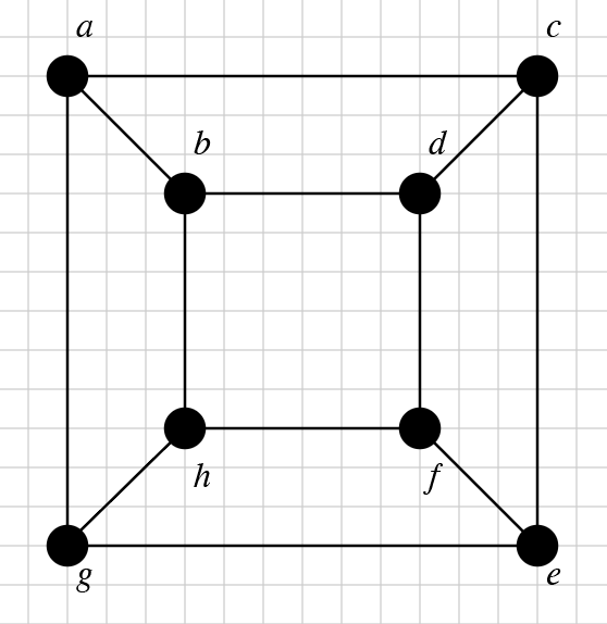
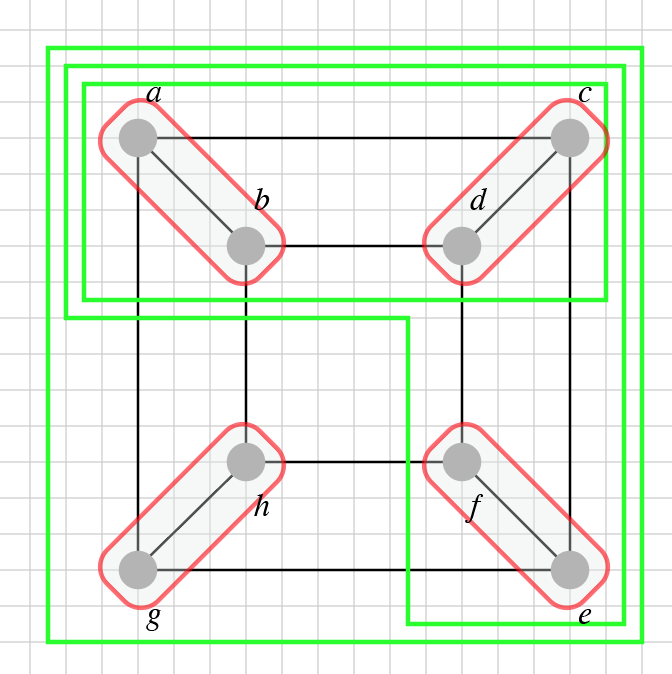
Figure 4: A $3$-regular plane graph (left) and the progression of algorithm $\mathsf{KS}$ on it (right). There are 4 ICT’s in this example, all single-edge, and all eligible for collapse of type-$b$.

Example 11.

In Figure 5 we show a $3$-regular plane graph decomposed into cycles and inter-cycle trees (ICT’s). In Figure 6 we show the progression of our algorithm $\mathsf{KS}$ on this graph. The five innermost super vertices enclosed in red boundaries on the left of Figure 6 are obtained from a first round of collapses (round 1 of $\mathsf{KS}$), followed by several merges (part of round 2 of $\mathsf{KS}$) that contract the self-loops of the five resulting super vertices. Actually, in this case, only the top super vertex among these five has self-loops to be contracted, shown as dashed edges on the left of Figure 6.

The remaining merges of round 2 contract several cycle edges, producing the two super vertices enclosed in green boundaries on the left of Figure 6. The four lower super vertices enclosed in red are put together to produce the lower super vertex in green on the left of Figure 6; this is result of three merge operations according to case 3 of condition $({\mathscr{D}}.1)$, followed by one more merge operation according to case 2 of condition $({\mathscr{D}}.1)$.

At this point, there remains only one ICT, with two ordinary vertices and two super vertices. One more round of collapses (round 3 of $\mathsf{KS}$) contracts this ICT into a super vertex with three self loops (the three remaining cycle edges that have not been yet contracted, shown as dashed edges on the right of Figure 6), and the latter are contracted by a final round of merges (round 4 of $\mathsf{KS}$) which produce the final super vertex shown on the right of Figure 6 enclosed in the outermost green boundary. $\square$

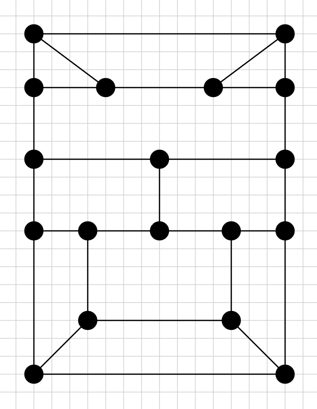
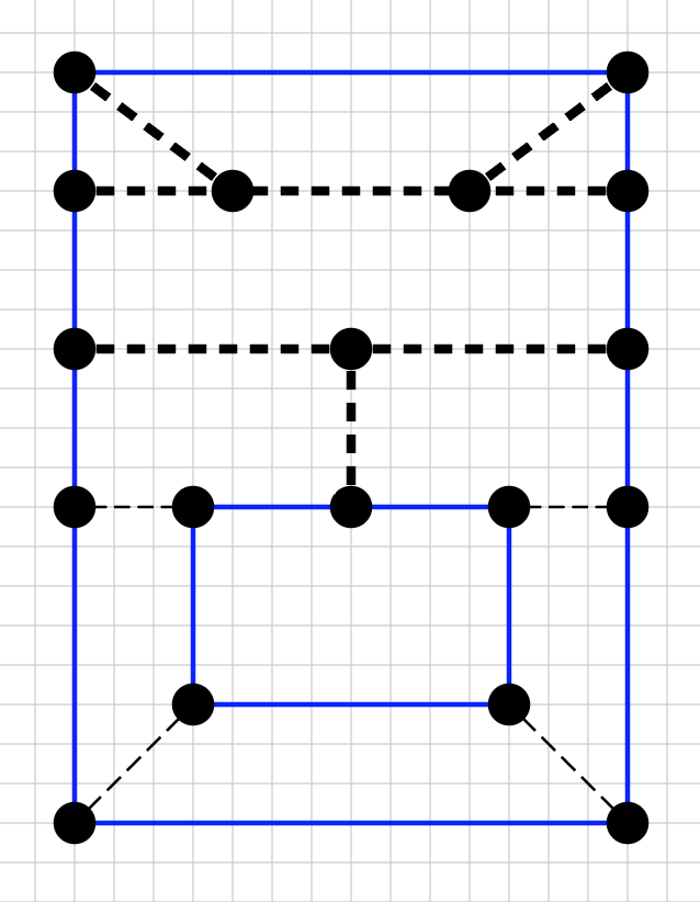
Figure 5: A $3$-regular plane graph (left figure) decomposed into $2$ cycles and $6$ ICT’s (right figure), $4$ ICT’s are single-edge (light dashed), $2$ multi-edge (bold dashed), only one not initially eligible for collapse (second from top).

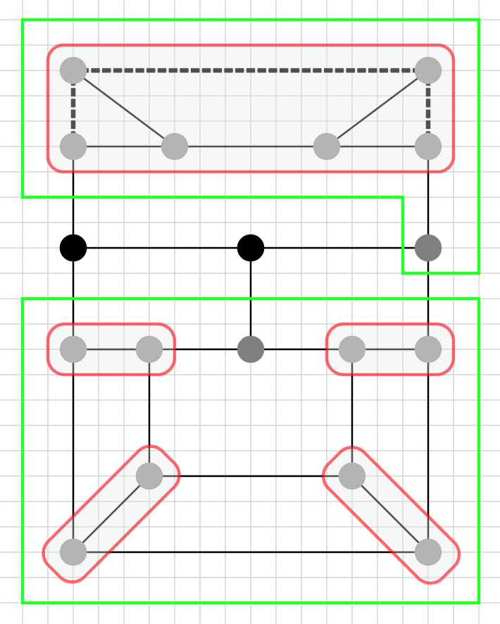
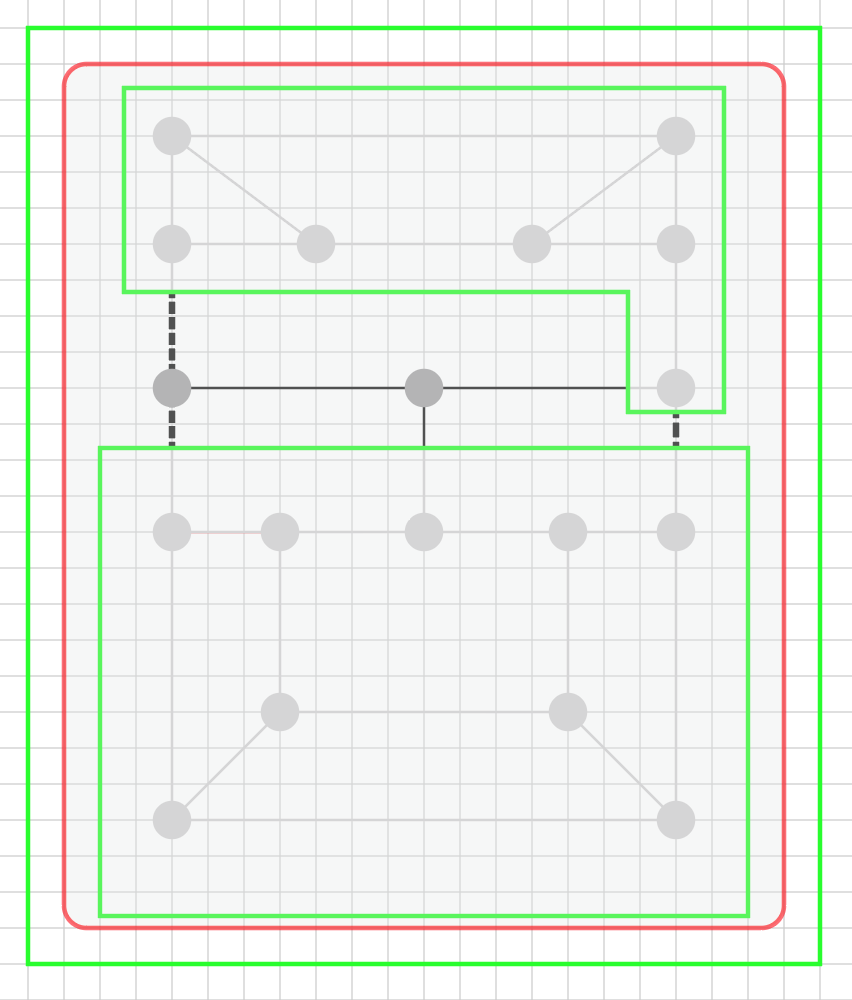
Figure 6: $\mathsf{KS}$’s progression on the graph in Figure 5. There is one ICT (left figure) with $2$ ordinary vertices (bold black) and $2$ super vertices (green), eligible for collapse (type-$a$) and contracted in $\mathsf{KS}$’s round 3 (right figure). $\mathsf{KS}$’s round 4 contracts the self-loops (dashed edges in right figure) and produces the last super vertex (green).

Example 12.

The graph in Figure 7 (on the left) is decomposed into $3$ cycles and $5$ ICT’s (on the right). The middle three-edge ICT is not initially eligible for collapse, and becomes eligible for collapse after rounds 1, 2, 3 and 4 (middle figure in Figure 8); and when it becomes eligible for collapse, it is a type-$a$ ICT, because its three leaf vertices (one ordinary and two super) are consecutive siblings on the same cycle. $\square$

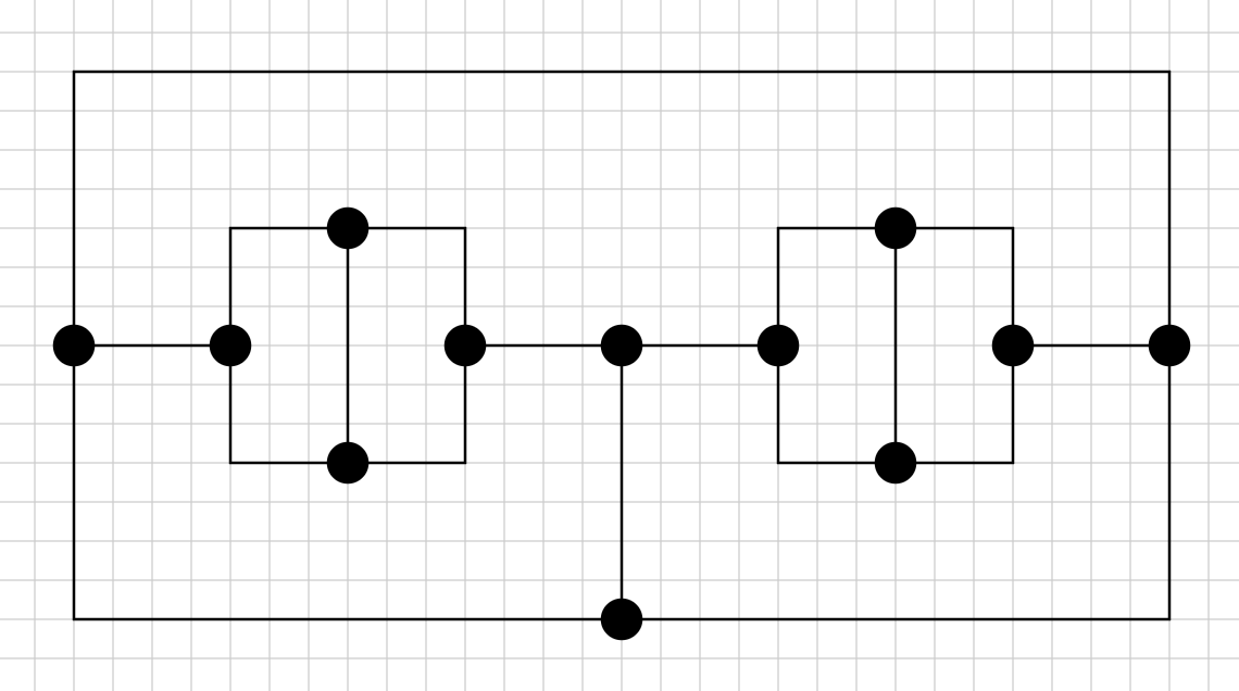
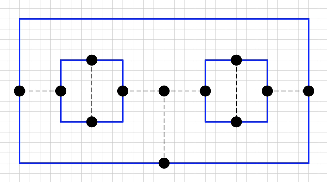
Figure 7: A $3$-regular plane graph (left figure) decomposed into $3$ cycles and $5$ ICT’s (right figure), $4$ ICT’s are single-edge, one is three-edge. Two single-edge ICT’s are initially eligible for collapse, the leftmost and the rightmost.

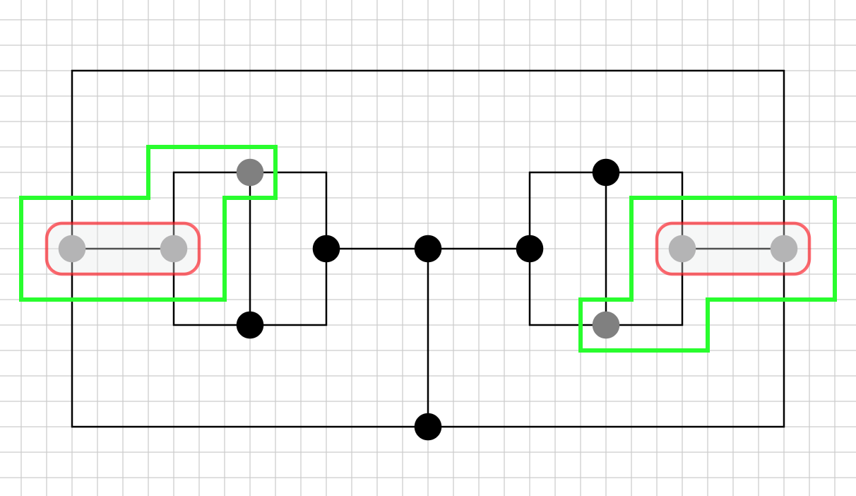
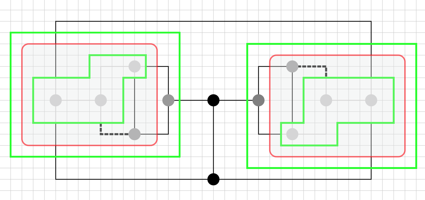
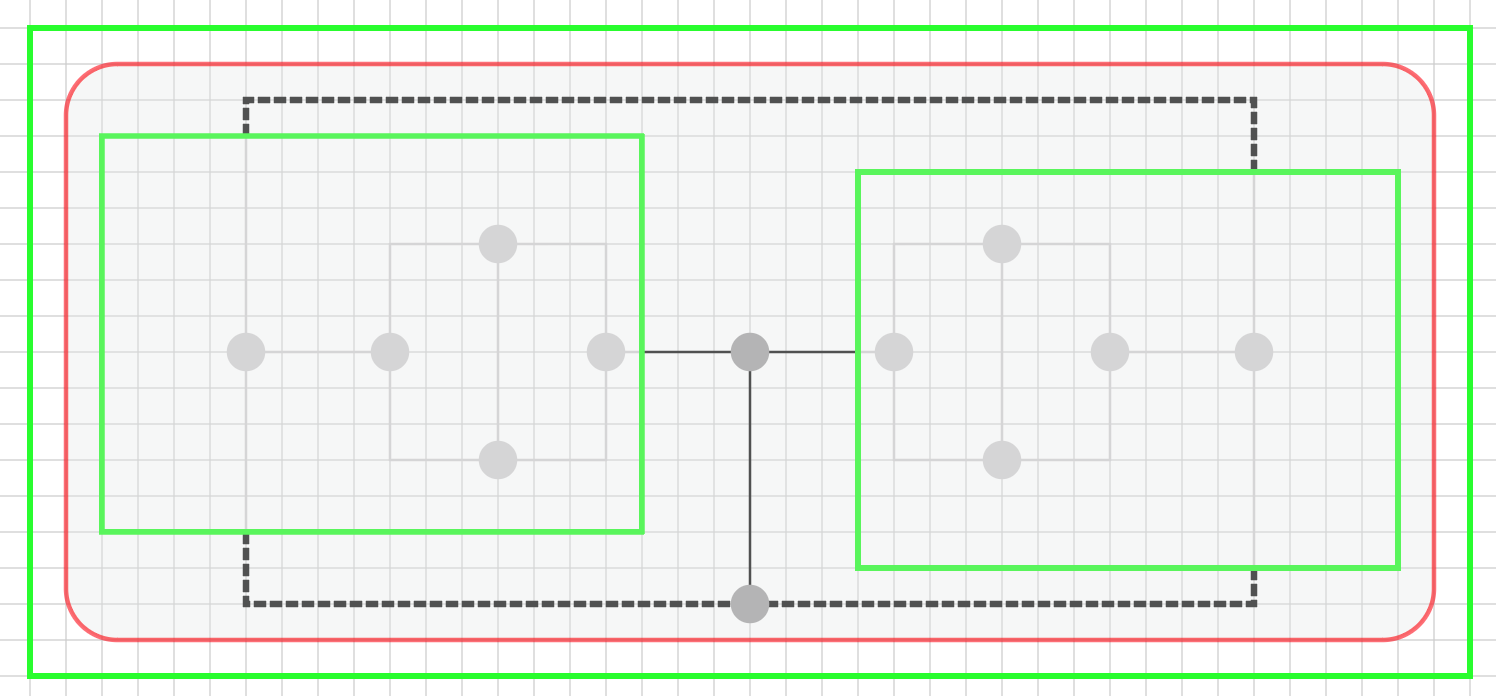
Figure 8: $\mathsf{KS}$’s progression on the graph in Figure 7, after rounds 1 and 2 (top left), rounds 3 and 4 (top right), and rounds 5 and 6 (bottom). $\mathsf{KS}$’s rounds 4 and rounds 6 contract two and three self-loops (dashed edges).

Example 13.

This is a variation on the graph in Example 12: All ICT’s are single-edge, except for one which is three-edge, just like in Example 12. Whereas the single three-edge ICT in Example 12 is type-$a$ when it becomes eligible for collapse (after round 4), the single three-edge ICT in this example is type-$b$ when it becomes eligible for collapse (after round 4). This illustrates how an ICT is classified as type-$a$ or type-$b$ dynamically, i.e., it is so classified at the time when it first becomes eligible for collapse. $\square$

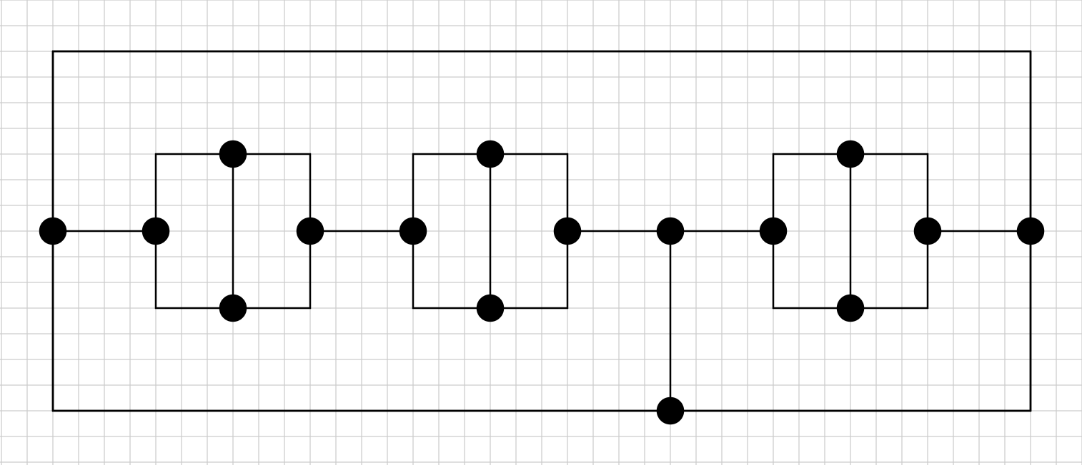
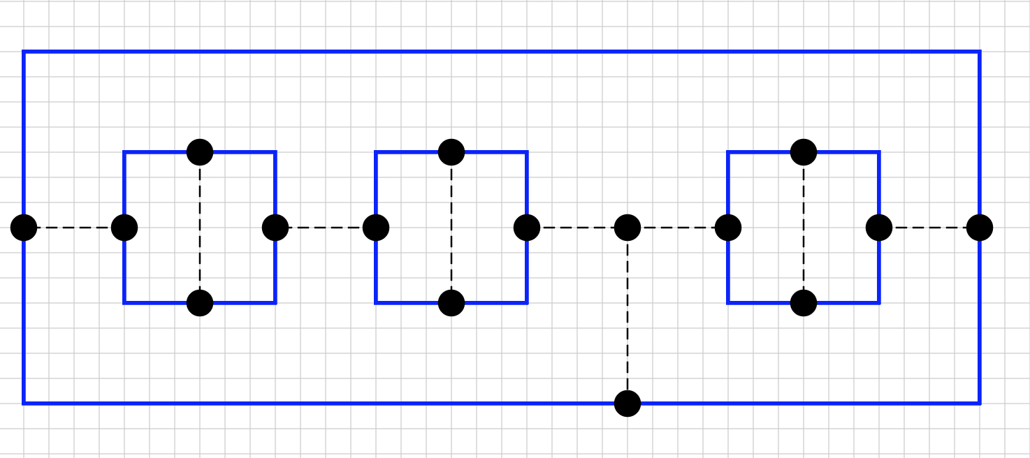
Figure 9: A $3$-regular plane graph (left) decomposed into $4$ cycles and $7$ ICT’s (right). One ICT is three-edge, $6$ ICT’s are single-edge, two of the latter initially eligible for collapse, the leftmost and the rightmost, both type-$b$.

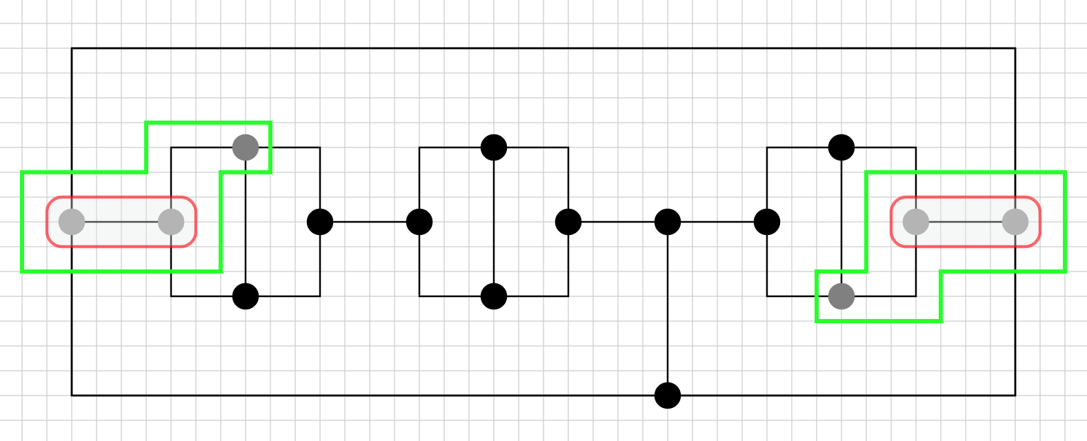
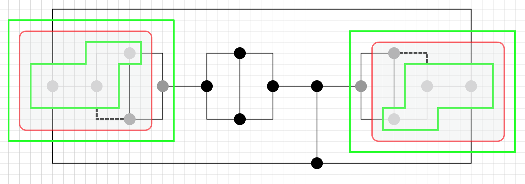
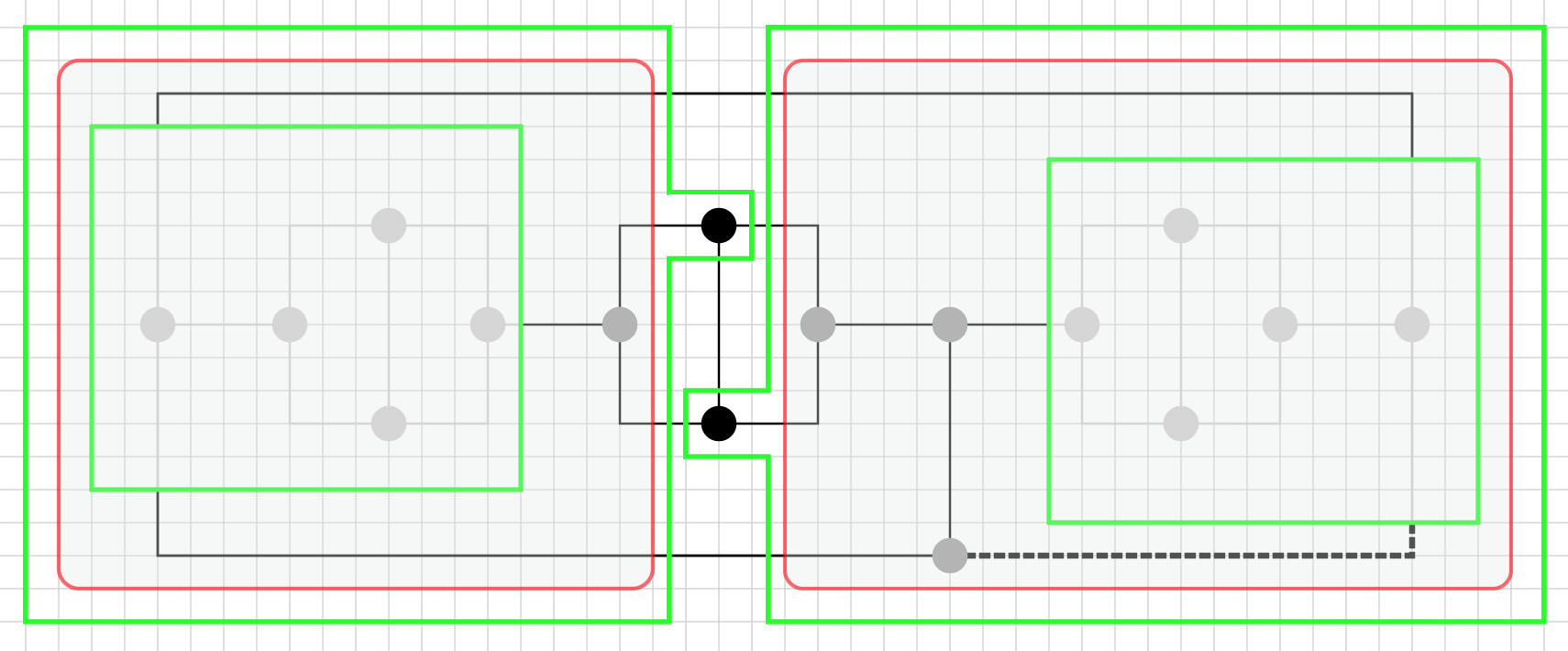
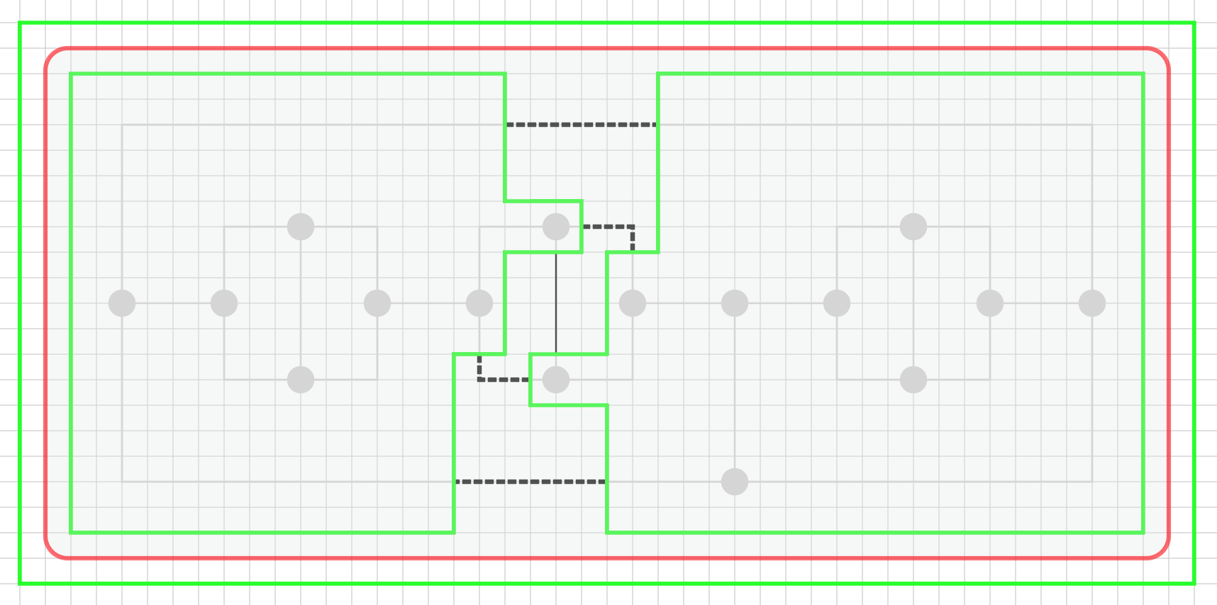
Figure 10: $\mathsf{KS}$’s progression on the graph in Figure 9, after rounds 1 and 2 (top figure), rounds 3 and 4 (second figure from top), rounds 5 and 6 (third figure from top), and rounds 7 and 8 (bottom figure). $\mathsf{KS}$’s rounds 4, rounds 6, and rounds 8, contract two, one, and four self-loops (dashed edges), respectively.

Example 14.

Figure 11 shows a $3$-regular plane graph with $54$ vertices, complicated enough to illustrate different aspects of our algorithm $\mathsf{KS}$. Figures 12 and 13 show the progression of algorithm $\mathsf{KS}$ on this graph.

On the left in Figure 12, the 14 innermost super vertices result from the first round of collapses (round 1 of $\mathsf{KS}$) which contract only ICT’s; these are enclosed in red boundaries. As a result of round 1, two self-loops are created, shown as dashed edges on the left in Figure 12. The following round of merges (round 2 of $\mathsf{KS}$) contracts the self-loops and produces 7 new super vertices, enclosed in green boundaries on the left in Figure 12. Six of these 7, enclosed in square green boundaries, are each obtained in two steps: first, by merging a super vertex with its clockwise neighbor, also a super vertex, according to case 3 of $({\mathscr{D}}.1)$; second, by merging the resulting super vertex with its clockwise neighbor, an outward ordinary vertex, according to case 2 of conditions $\{({\mathscr{D}}.1),({\mathscr{D}}.2)\}$. The remaining super vertex in green of those 7, on the left in Figure 12, is obtained by merging a super vertex with its clockwise neighbor, an inward ordinary vertex, according to case 1 of $({\mathscr{D}}.1)$.

Out of the 14 innermost super vertices in red on the left in Figure 12, one is not involved in any contractions of round 2 (i.e., first round of merges); conditions $\{({\mathscr{D}}.1),({\mathscr{D}}.2)\}$ and their 5 special cases do not apply to it.

The next round of collapses (round 3 of $\mathsf{KS}$) produces the super vertices enclosed in red boundaries on the right in Figure 12. There are 8 of these super vertices, 7 new and 1 from round 1 that was not involved in any contractions in the intermediate round 2. Also on the right in Figure 12, three new super vertices in green boundaries are shown, resulting from the following round of merges (round 4 of $\mathsf{KS}$).

The result of the next round of collapses and the following round of merges, round 5 and round 6 of $\mathsf{KS}$ respectively, is shown on the left in Figure 13. At this point, all the ordinary vertices in the initial graph are included in one of two disjoint super vertices. The latter two super vertices are connected by two cycle edges and one inter-cycle edge; these are the three remaining uncontracted edges.

The contraction of that last inter-cycle edge is the result of one more round of collapses, round 7 of $\mathsf{KS}$, which creates two self-loops from the two remaining uncontracted cycle edges (shown as dashed edges on the right in Figure 13). The latter are contracted by one more round of merges, round 8 of $\mathsf{KS}$. $\square$

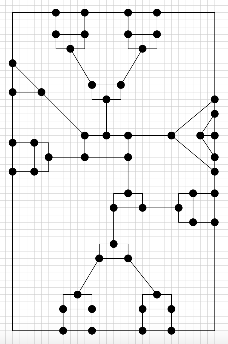
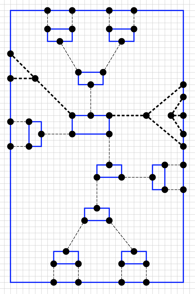
Figure 11: A $3$-regular plane graph (left) decomposed into 11 cycles and 24 ICT’s (right), 21 ICT’s are single-edge (light dashed edges) and 3 are multi-edge (bold dashed edges). Fourteen of the 24 initial ICT’s are eligible for collapse; of these 14, one ICT is type-$a$ (nested multi-edge on the right), and 13 ICT’s are type-$b$.

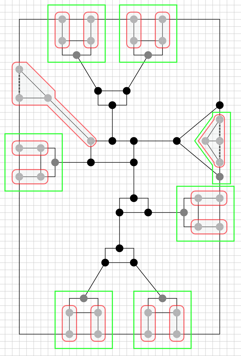
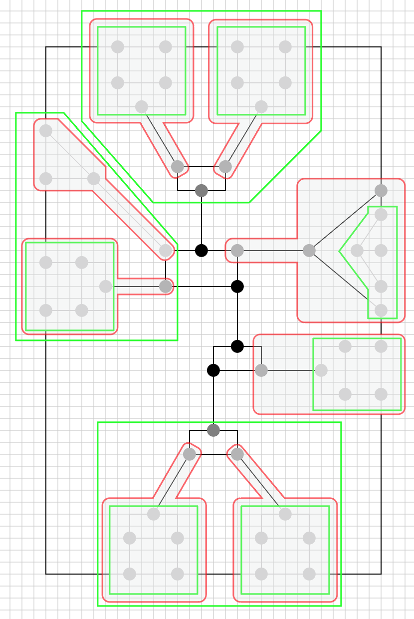
Figure 12: Progression of algorithm $\mathsf{KS}$ on the graph in Figure 11. All ICT’s eligible for collapse on the left, 7 of them, are type-$b$. All ICT’s eligible for collapse on the right, 2 of them, are type-$b$; one of these two involves the topmost super vertex, the other involves the bottommost super vertex.

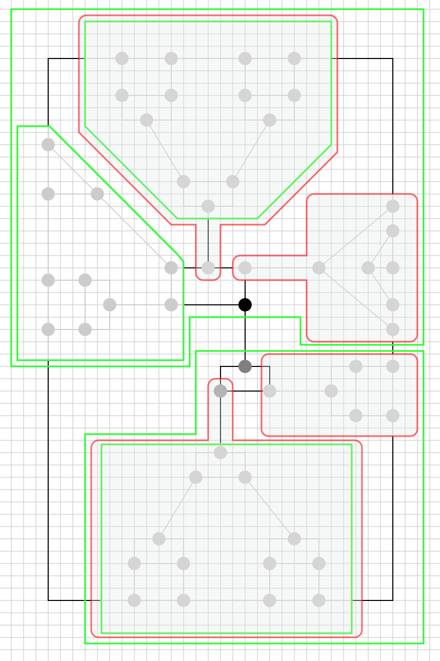
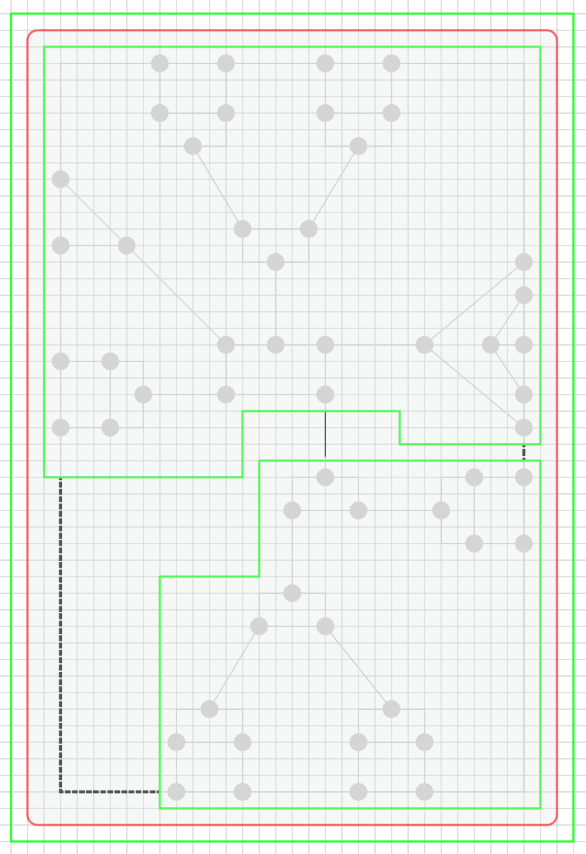
Figure 13: Progression of algorithm $\mathsf{KS}$ on the graph in Figures 11 and 12. There is only one (single-edge) ICT on the left which is type-$a$ and eligible for collapse. There are no ICT’s on the right.

Example 15.

In Figure 14 is a $3$-regular plane graph with $42$ vertices, again complicated to exhibit additional aspects of our algorithm $\mathsf{KS}$. The top of Figure 14 shows the initial input graph $G$, and the bottom shows $G$’s decomposition into $5$ cycles and $18$ ICT’s. In this case, it is easy to see that ${{E}\text{-}\mathsf{outerplanarity}}(G)=4$.

The progression of algorithm $\mathsf{KS}$ is shown in Figure 15. The top of the figure shows the result of round 1 of collapses ($7$ of them) followed by round 2 of merges (also $7$ of them). Super vertices resulting from round 1 are enclosed in red boundaries, and super vertices resulting from round 2 are enclosed in green boundaries. There are only $6$ super vertices shown in green, not $7$, because one of them (at the north-west corner of the graph) is obtained by two merges: the first according to case 3 of condition $({\mathscr{D}}.1)$ and the second according to case 1 of condition $({\mathscr{D}}.1)$.

The middle of Figure 15 shows the result of round 3 of collapses followed by round 4 of merges. As in the two previous rounds, super vertices resulting from collapses are enclosed in red boundaries ($9$ such boundaries) and super vertices resulting from merges are enclosed in green boundaries ($7$ such boundaries). Two of the $7$ super vertices in green are each the result of two consecutive merges, one according to case 3 of condition $({\mathscr{D}}.1)$ followed by one according to case 1 of condition $({\mathscr{D}}.1)$; these two super vertices in green are at the north-west corner of the graph in the middle of Figure 15 and at the south-center in the middle of the same figure.

One of the merges from round 4 does not create a new super vertex; it only contracts self-loops, shown as dashed edges in the middle graph in Figure 15. A merge operation that contracts self-loops is one according to case 5 of condition $({\mathscr{D}}.1)$.

At this point, there are only two ICT’s that have not yet been contracted. Each of these two consists of a single ordinary vertex (shown as a boldface vertex in the middle graph in Figure 15) and three super vertices that share a same innermost cycle.

The bottom of Figure 15 shows the result of round 5 of collapses (two of them) followed by round 6 of merges (four of them). The two collapses produce two super vertices, enclosed in red boundaries at the bottom of Figure 15, each with $5$ self-loops, shown as dashed edges. These $10$ self-loops are contracted by two merges according to case 5 of condition $({\mathscr{D}}.1)$. There are now $3$ super vertices, connected by a total of $5$ cycle edges that are yet to be contracted. A merge according to case 3 of condition $({\mathscr{D}}.1)$, followed by a merge according to case 4 of condition $({\mathscr{D}}.1)$, contract these $5$ cycle edges and produce the final and only super vertex. $\square$

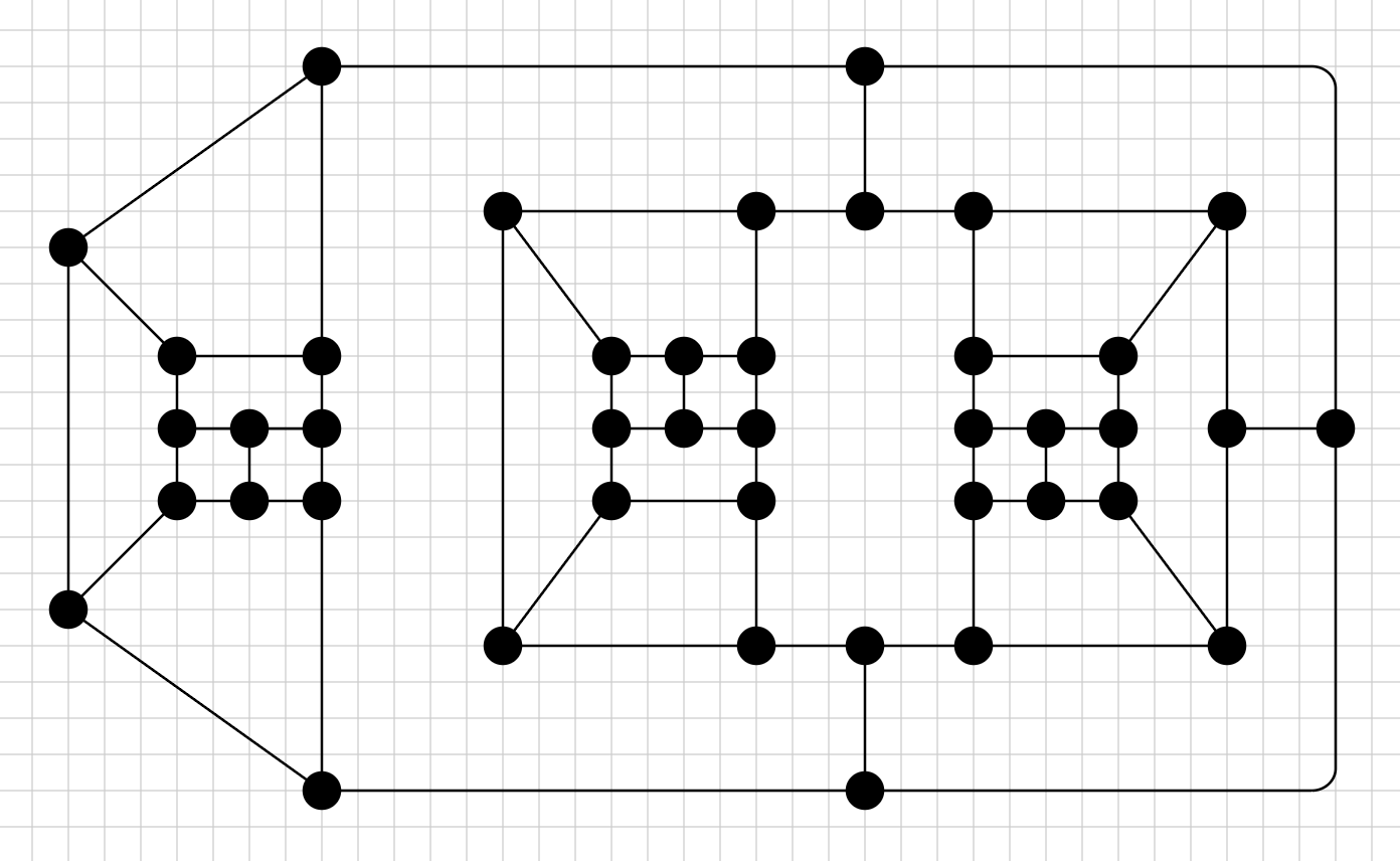
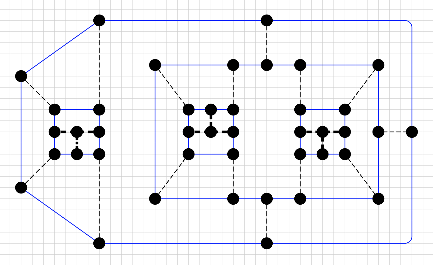
Figure 14: A $3$-regular plane graph (left) decomposed into 5 cycles and 18 ICT’s (right), 15 ICT’s are single-edge (light dashed) and 3 multi-edge (bold dashed). Seven of the 18 initial ICT’s are eligible for collapse, all type-$b$.

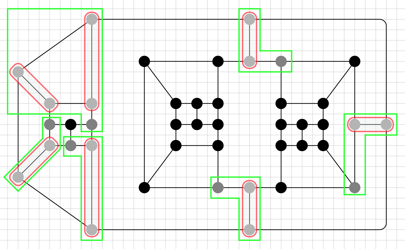
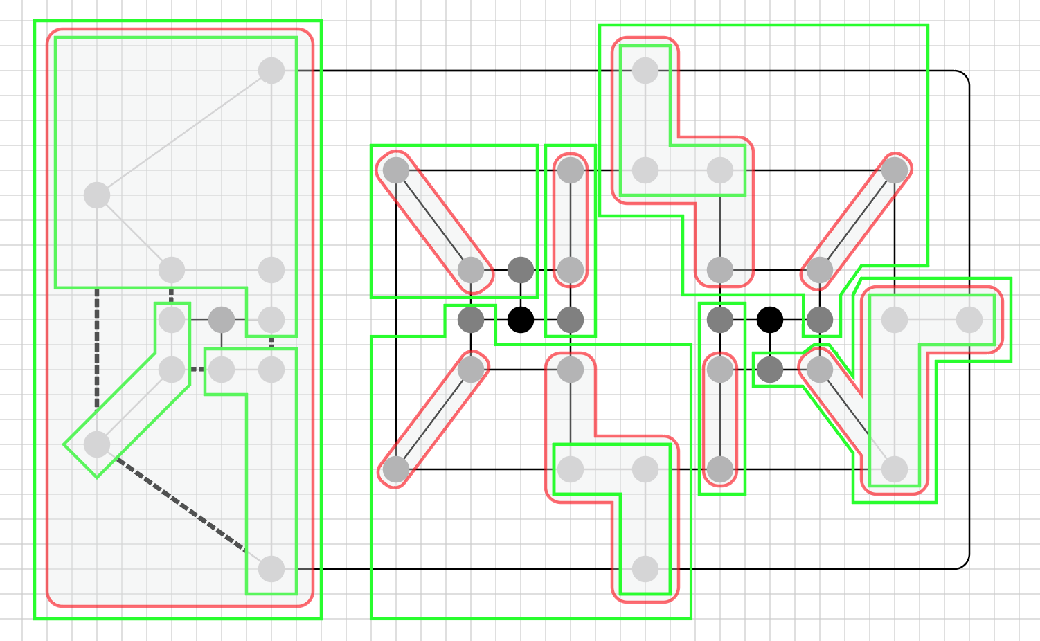
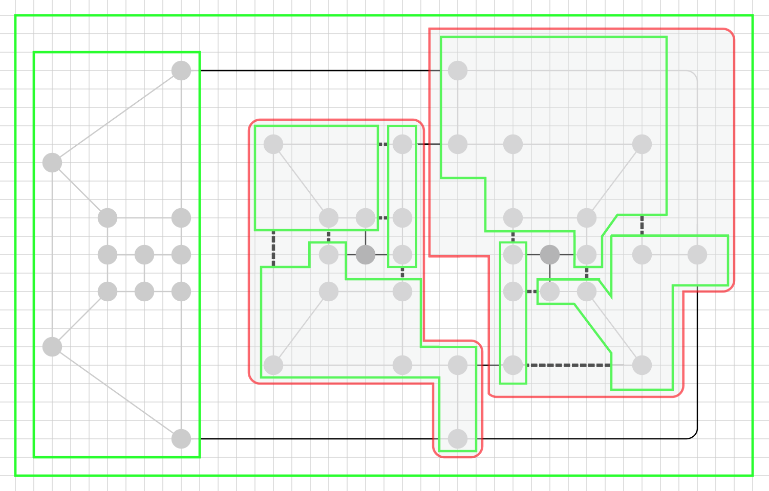
Figure 15: $\mathsf{KS}$’s progression on the graph in Figure 14. The top figure shows the graph after rounds 1 and 2, the middle figure after rounds 3 and 4, and the bottom figure after rounds 5 and 6. In the top figure, there are 9 ICT’s eligible for collapse; 8 of these are single-edge and type-$b$, and one (at the west) is multi-edge and type-$a$. In the middle figure, there are 2 ICT’s eligible for collapse, both multi-edge and type-$a$. In the bottom figure, there are no ICT’s eligible for collapse.

4.6 Proof of Correctness and Complexity

We prove the correctness of our algorithm $\mathsf{KS}$ by referring to the conditions $\mathscr{C}$ for collapses (Section 4.3) and the conditions $\mathscr{D}$ for merges (Section 4.4). We purposely avoid any explicit reference to the pseudocode in Appendix A for two reasons: first, any such reference would obscure the intuition underlying the proofs of Lemmas 16, 17, 18, and 19, as well as an informal understanding of their correctness; second, the pseudocode in Appendix A proposes one particular way (there are others) of implementing $\mathsf{KS}$ and programming the conditions in $\mathscr{C}$ and $\mathscr{D}$.

Let $G$ be a biconnected $3$-regular simple plane graph as in Theorem 9. The execution of our algorithm can be represented by a sequence of graphs (multigraphs after the first $G_{0}$):

• $G_{0}=G\quad\ G_{1}\quad\ G_{2}\quad\ G_{3}\quad\ \ldots\ \ \quad\ G_{i}\quad\ G_{i+1}\ \ \ldots\ \ \quad\ G_{p}$

where for every odd $i\geqslant 1$ (resp. even $i\geqslant 2$), graph $G_{i}$ is obtained from the preceding $G_{i-1}$ by a maximum round of collapses (resp. merges). Thus, round 1 is a round of collapses, round 2 is a round of merges, round 3 is a round of collapses, etc. This sequence is bound to terminate after a finite number $p$ of rounds, because the collapse and merge operations contract edges and there are finitely many edges. We say the sequence $(\spadesuit)$ terminates successfully if the last graph $G_{p}$ is a single super vertex with no edges. We use Lemma 16 to prove Part 1 of Theorem 9.

Lemma 16.

The sequence $(\spadesuit)$ terminates successfully.

Proof.

We prove the lemma by contradiction. Assume the sequence $(\spadesuit)$ does not terminate successfully, i.e.:

1. $\widetilde{G}=G_{p}$ is not a single super vertex, and

2. no collapse operation and no merge operation can be applied to $\widetilde{G}$.

For an easy case first, assume that there are no ICT edges in $\widetilde{G}$, because they have all been contracted in earlier rounds, and that all the edges left in $\widetilde{G}$ are cycle edges. An ICT $T$ before a collapse operation, whether of type-$a$ or type-$b$ (see Remark in Section 4.3), has at least one ordinary vertex; after $T$’s collapse, all of it vertices, ordinary or super, become merged into a single super vertex. Hence, all vertices in $\widetilde{G}$ are now super vertices. Consider an innermost cycle $X$ in $\widetilde{G}$. Then $X=\mathsf{innermost}\text{-}\mathsf{cycle}(\varphi)$ for some super vertex $\varphi$. If there is no super vertex $\psi\neq\varphi$ such that $X=\mathsf{innermost}\text{-}\mathsf{cycle}(\psi)$, then $X$ is a self-loop of $\varphi$, otherwise we can choose $\psi$ as the clockwise neighbor of $\varphi$. In either case, a round of merges can be applied to $\widetilde{G}$, contradicting our initial assumption.

Assume next that there is an ICT $T$ which has not been collapsed in $\widetilde{G}$. Let all of $T$’s leaf vertices, except possibly for one outward ordinary $w$ in case $T$ is of type-$b$, be siblings on a cycle $X$, which are necessarily super vertices or inward ordinary vertices. Among all ICT $T^{\prime}\neq T$ in $\widetilde{G}$ that have not been collapsed, select $T$ so that $\mathsf{level}(X)\leqslant\mathsf{level}(X^{\prime})$ where $X^{\prime}$ is the cycle on which the leaf vertices of $T^{\prime}$ are located. Hence, there are no ordinary outward vertices on $X$, because any such ordinary outward vertex would be the root of a type-$b$ ICT $T^{\prime}$ incident to $X$ from the outside and such that: (i) $T^{\prime}$ has not been collapsed and (ii) $\mathsf{level}(X^{\prime})<\mathsf{level}(X)$, which would contradict the conditions for our selection of $T$.

Moreover, all the super vertices on $X$ must be leaf vertices of ICT’s enclosed in $X$, i.e., ICT’s that are incident to $X$ from the inside of $X$. Indeed, if any of these super vertices, say $\varphi$, were not a leaf vertex of any such enclosed ICT, it would be possible to apply the merge operation to contract the cycle edge connecting $\varphi$ with its clockwise neighbor on $X$ and $\widetilde{G}$ would not be the last graph in the sequence $(\spadesuit)$. Hence, it follows that:

• all the vertices on $X$ are either super vertices or ordinary inward vertices, and all of them are leaf vertices of ICT’s that are enclosed in $X$.

If all the leaf vertices of the selected $T$ are consecutive siblings on $X$, it contradicts the assumption that no collapse operation can be applied to $\widetilde{G}$. So, the leaf vertices of $T$ cannot be consecutive on $X$. But from this, together with fact ($), it is easy to argue there must be another ICT $T_{0}$ whose leaf vertices are consecutive siblings on $X$, implying again that the collapse operation can be applied to $\widetilde{G}$. We conclude that the sequence $(\spadesuit)$ always terminate successfully. ∎

We use Lemma 17 in the proof of Lemma 18, and we use the latter to prove Part 2 of Theorem 9. In the lemmas to follow, $G$ is possibly a plane multigraph resulting from earlier applications of the collapse and merge operations.

Lemma 17.

Let $T$ be an ICT in $G$ satisfying condition $({\mathscr{C}}.2)$ all of whose leaf vertices, except possibly for one outward ordinary $w$, are consecutive siblings on a cycle $X$. Let $M=\{\mu_{1},\ldots,\mu_{p}\}$ be the consecutive siblings on $X$, each of which is a super vertex or an inward ordinary vertex. Assume none of the super vertices in $M$ have self-loops (as a result of preceding merge operations). It then holds that:

1. For every super vertex $\varphi$ in $G$, if its clockwise neighbor is a super vertex $\psi\in M$, then $\varphi\in M$ ($\varphi$ is thus a leaf vertex of $T$); in which case $\mathsf{innermost}\text{-}\mathsf{cycle}(\varphi)=\mathsf{innermost}\text{-}\mathsf{cycle}(\psi)=X$ and there are no ordinary vertices on $X$ between $\varphi$ and $\psi$.

2. For every leaf vertex ${\mu}_{i}\in M$, the set $\mathsf{cycles}({\mu}_{i})$ is a chain of nested cycles of consecutive levels, with $\mathsf{level}(X)$ being the highest level and $X$ being its innermost cycle.

3. For all leaf vertices ${\mu}_{i},{\mu}_{j}\in M$, it holds that $\mathsf{cycles}({\mu}_{i})\subseteq\mathsf{cycles}({\mu}_{j})$ or $\mathsf{cycles}({\mu}_{i})\supseteq\mathsf{cycles}({\mu}_{j})$.

Proof.

For Part1, let $\mathsf{innermost}\text{-}\mathsf{cycle}(\varphi)=Y$. If $\psi$ is the clockwise neighbor of $\varphi$, then $Y\in\mathsf{cycles}(\psi)$. If $Y\neq X=\mathsf{innermost}\text{-}\mathsf{cycle}(\psi)$, then $\varphi$ would be merged with $\psi$ in a preceding round of merge operations. Hence, if $\varphi$ and $\psi$ are distinct, it must be that $Y=X$. And since $\psi$ is $\varphi$’s clockwise neighbor, there are no intervening ordinary vertices on $X$ between $\varphi$ and $\psi$.

We can prove Part 2 by induction on the number $q\geqslant 1$ of rounds of applying the collapse operation on the initial simple three-regular plane graph. For $q=1$, the desired conclusion is immediate, because all the leaf vertices of ICT’s that are eligible for collapse in the initial graph are ordinary vertices, and each of these ordinary vertices straddles exactly one cycle. For the induction hypothesis, we assume the conclusion holds for an arbitrary $q\geqslant 1$ rounds of collapses interleaved with $q$ rounds of merges, and we next prove the conclusion after the $(q+1)$-st round of collapses is applied. The $q$-th round of merges, immediately preceding the $(q+1)$-st round of collapses, contracts all self-loops of the same vertex.

Suppose the $(q+1)$-st round of collapses results in the contraction of an ICT $T$ with leaf vertices $M=\{\mu_{1},\ldots,\mu_{p}\}$ or $M\cup\{w\}=\{\mu_{1},\ldots,\mu_{p}\}\cup\{w\}$, depending on whether $T$ is type-$a$ or type-$b$ (see Remark in Section 4.3), with $X$ being the innermost cycle of all the members of $M$ and $X^{\prime}$ being the sole cycle of $w$. The contraction of such an ICT $T$ into a super vertex $\chi$ generally creates self-loops of $\chi$. The self-loops thus created, if any, are all edges of cycles in the chain of nested cycles formed by the members of $\bigcup\{\,\mathsf{cycles}(\mu_{i})\;|\;\mu_{i}\in M\,\}$. Suppose this chain of nested cycles is:

$$X_{1},\ \ldots\ ,\ X_{r},\ X_{r+1},\ \ldots\ ,\ X_{r+s},\ X_{r+s+1},\ \ldots\ ,\ X_{r+s+t}$$

with $X=X_{r+s+t}$, which is listed in order of increasing consecutive levels and divided into three groups:

• $\{X_{1},\ldots,X_{r}\}$ do not contribute self-loops of $\chi$ and are included in $\mathsf{cycles}(\chi)$,

• $\{X_{r+1},\ldots,X_{r+s}\}$ contribute self-loops of $\chi$ and are included in $\mathsf{cycles}(\chi)$,

• $\{X_{r+s+1},\ldots,X_{r+s+t}\}$ contribute self-loops of $\chi$ and are not included in $\mathsf{cycles}(\chi)$, because all their edges are turned into self-loops.

After applying the $(q+1)$-st round of merges, the self-loops of $\chi$, all necessarily of levels $\geqslant\mathsf{level}(X^{\prime})$, are eliminated by contraction. Let $\chi^{\prime}$ be $\chi$ after the elimination of all self-loops. If $T$ is a type-$a$, then $\mathsf{cycles}(\chi^{\prime})=\{X_{1},\ldots,X_{r+s}\}$ and $\mathsf{innermost}\text{-}\mathsf{cycle}(\chi^{\prime})=X_{r+s}$. If $T$ is a type-$b$, it is not difficult to check that $\mathsf{level}(X^{\prime})=1+\mathsf{level}(X_{r+s})$, with $\mathsf{cycles}(\chi^{\prime})=\{X_{1},\ldots,X_{r+s}\}\cup\{X^{\prime}\}$ so that also $\mathsf{innermost}\text{-}\mathsf{cycle}(\chi^{\prime})=X^{\prime}$. This implies the conclusion of Part 2.

For Part 3, if ${\mu}_{i}$ or ${\mu}_{j}$ is an ordinary vertex, then the conclusion is immediate, because $X$ is the sole cycle of all the ordinary vertices in $M$ and $X$ is also the innermost cycle of all the vertices in $M$. Suppose next that neither ${\mu}_{i}$ nor ${\mu}_{j}$ are ordinary vertices and, by way of getting a contradiction, that $\mathsf{cycles}({\mu}_{i})\not\subseteq\mathsf{cycles}({\mu}_{j})$ and $\mathsf{cycles}({\mu}_{i})\not\supseteq\mathsf{cycles}({\mu}_{j})$. Hence, there are cycles $Y_{i}\in\mathsf{cycles}({\mu}_{i})$ and $Y_{j}\in\mathsf{cycles}({\mu}_{j})$ such that $Y_{i}\not\in\mathsf{cycles}({\mu}_{j})$ and $Y_{j}\not\in\mathsf{cycles}({\mu}_{i})$. But cycles $Y_{i}$ and $Y_{j}$ both enclose cycle $X$, and each of $\mathsf{cycles}({\mu}_{i})$ and $\mathsf{cycles}({\mu}_{j})$ is a set of nested cycles of consecutive levels. Since cycles $Y_{i}$ and $Y_{j}$ cannot cross each other, it must be that either $Y_{i}$ is nested in $Y_{j}$ or $Y_{j}$ is nested in $Y_{i}$, i.e., $Y_{i}\in\mathsf{cycles}({\mu}_{j})$ or $Y_{j}\in\mathsf{cycles}({\mu}_{i})$ – but this is a contradiction. ∎

Lemma 18.

Let $T$ be an ICT in $G$ satisfying condition $({\mathscr{C}}.2)$ all of whose leaf vertices, except possibly for one outward ordinary $w$, are consecutive siblings on a cycle $X$. Let $M=\{\mu_{1},\ldots,\mu_{p}\}$ be the consecutive siblings on $X$, with $p\geqslant 1$, each of which is a super vertex or an inward ordinary vertex. Let $N=\{v_{1},\ldots,v_{q}\}$ be the non-leaf vertices of $T$, which are all ordinary of degree $3$, with $q\geqslant 0$. Assume none of the super vertices in $M$ have self-loops (as a result of preceding merge operations).

It then holds that there is an algorithm Collapse which on input $T$ returns in linear time ${\cal O}\bigl{(}p+q\bigr{)}$ a reassembling of $T$, i.e., $\textsc{Collapse}(T)={\cal B}$ where ${\cal B}$ is a binary reassembling of the vertices in $M\cup N$ (if $T$ is type-$a$) or in $M\cup N\cup\{w\}$ (if $T$ is type-$b$) such that:

1. $\alpha(T,{\cal B})\leqslant 3$.

2. $\alpha(G,{\cal B})\leqslant 1+\max\,\bigl{\{}\,{\mathit{deg}}_{G}(\mu_{i})\;\big{|}\;\mu_{i}\in M\,\bigr{\}}$.

3. If $\varphi$ is the super vertex resulting from contracting all the edges of $T$, and $\psi$ is the super vertex resulting from contracting all the self-loops of $\varphi$, then

   $${\mathit{deg}}_{G}(\psi)\ \leqslant\ \begin{cases}\max\,\bigl{\{}\,{\mathit{deg}}_{G}(\mu_{i})\;\big{|}\;\mu_{i}\in M\,\bigr{\}}&\text{if $T$ is type-$a$},\\[2.97083pt] 2+\max\,\bigl{\{}\,{\mathit{deg}}_{G}(\mu_{i})\;\big{|}\;\mu_{i}\in M\,\bigr{\}}\qquad&\text{if $T$ is type-$b$}.\end{cases}$$

Proof.

We first define a traversal of $T$, which includes all the tree edges of $T$ and excludes all the cycle edges connecting its leaf vertices $\{\mu_{1},\ldots,\mu_{p}\}$ or $\{\mu_{1},\ldots,\mu_{p}\}\cup\{w\}$, depending on whether $T$ is type-$a$ or type-$b$, respectively. The traversal starts at any of the leaf vertices, say $\mu_{1}$, and moves along the edge, call it $e_{1}$, that connects $\mu_{1}$ to a non-leaf vertex, say $v_{1}$. From $v_{1}$ (and from every subsequent non-leaf vertex), the traversal continues recursively by visiting the left subtree (first), then the right subtree (second), and then finally edge $e_{1}$ in the reverse direction from $v_{1}$ to $\mu_{1}$ (third). It is easy to check that this traversal visits the starting leaf vertex $\mu_{1}$ twice, every non-leaf vertex three times, and every other leaf vertex in $\{\mu_{2},\ldots,\mu_{p}\}$ or $\{\mu_{2},\ldots,\mu_{p}\}\cup\{w\}$ once, and can be carried out in time ${\cal O}\bigl{(}p+q\bigr{)}$. As the traversal proceeds recursively, it is useful to think that every non-leaf vertex $v_{j}$ with $1\leqslant j\leqslant q$, which is first reached by traversing an edge, say $e_{j}$, is the root of a binary tree whose right and left subtrees are the subtrees that can be aligned with edge $e_{j}$ by a counterclockwise and a clockwise rotation around $v_{j}$, respectively.

Algorithm Collapse carries out the traversal of $T$ just defined and simultaneously builds the vertex clusters of a binary reassembling ${\cal B}$ as in the statement of the lemma. It builds a singleton cluster $X_{i}\triangleq\{\mu_{i}\}$ the first time it visits leaf vertex $\mu_{i}$, which is also the only time for $i\in\{2,\ldots,p\}$. If $T$ is a type-$b$ and $w$ exists, it also builds a singleton cluster $X_{p+1}\triangleq\{w\}$ the first and only time it visits leaf vertex $w$. For every non-leaf vertex $v_{j}$, algorithm Collapse builds a cluster $X_{j}$ where $1\leqslant j\leqslant q$ right after it visits $v_{j}$ the third and last time; the desired $X_{j}$ is defined as:

$$X_{p+j}\ \triangleq\ \{v_{j}\}\cup Y\cup Z\quad\text{or}\quad X_{p+1+j}\ \triangleq\ \{v_{j}\}\cup Y\cup Z,$$

depending on whether $T$ is type-$a$ or type-$b$, where $Y$ and $Z$ are the clusters of all the vertices (both leaf and non-leaf) of the right and left subtrees of $v_{j}$, respectively.

Part 1 of the lemma now readily follows from the preceding analysis. Part 2 is an easy consequence of Part 1. In Part 1, the degree of every leaf vertex is one because $T$ is considered in isolation from the rest of $G$; in Part 2, the degrees of the leaf vertices (also cycle vertices in $G$) are ${\mathit{deg}}_{G}(\mu_{1}),\ldots,{\mathit{deg}}_{G}(\mu_{p})$ and ${\mathit{deg}}_{G}(w)=3$.

Part 3 is a straightforward consequence of Lemma 17. If $T$ is type-$b$, let $\mathsf{cycles}(w)=X^{\prime}$ which is necessarily $\neq X$, in which case $\mathsf{level}(X^{\prime})=1+\mathsf{level}(X)$. Whether $T$ is type-$a$ or type-$b$, it is easy to see that:

$$\mathsf{cycles}(\psi)\ =\ \mathsf{cycles}(\varphi)\ -\ \{\;\text{all the self-loops of $\varphi$}\;\}$$

where $\mathsf{cycles}(\varphi)=\bigcup\{\mathsf{cycles}({\mu}_{i})|\mu_{i}\in M\}$ or $\mathsf{cycles}(\varphi)=\{X^{\prime}\}\cup\bigcup\{\mathsf{cycles}({\mu}_{i})|\mu_{i}\in M\}$, depending on whether $T$ is type-$a$ or type-$b$, respectively. ∎

For the next lemma, review the pre-processing phase and processing phase of algorithm $\mathsf{KS}$ in Section 4.1.

Lemma 19.

The pre-processing phase and processing phase of $\mathsf{KS}$ on graph $G$ are each carried out in ${\cal O}(n)$ steps, each using ${\cal O}(n)$ space, where $n=|\,\mathbf{V}(G)\,|$.

Proof.

The initial input graph $G$ is represented by an adjacency list, where each vertex $v$ is identified by a pair of numbers ($v$’s coordinates in the Cartesian plane) together with a list containing the three vertices to which $v$ is connected. This requires ${\cal O}(n)$ space. The pre-processing phase decomposes the input graph $G$ into ICT’s and cycles at each level of edge-outerplanarity, where every ICT can be identified by a postorder traversal (left, right, root); this whole pre-processing does not need to exceed ${\cal O}(n)$ time and ${\cal O}(n)$ space for its work.

In the processing phase, every ICT $T$ is collapsed in time linear in the size $|\,T\,|$; this is the result of $\textsc{Collapse}(T)$ in Lemma 18 which, according to its proof, also uses a postorder traversal (left, right, root). All vertices (including all cycle vertices), whether ordinary or super, are each part of exactly one ICT, and every ICT is collapsed exactly once. Because any reassembling can be viewed as a tree containing $(2n-1)$ nodes (review definitions of reassembling trees in Section 2), corresponding to $n$ initial ordinary vertices plus $(n-1)$ super vertices produced in the course of $\mathsf{KS}$’s operation, the entire processing phase also takes ${\cal O}(n)$ time and ${\cal O}(n)$ space. ∎

Proof of Theorem 9.

Part 1 of Theorem 9 is an immediate consequence of Lemma 19. Lemma 16, Lemma 17, and Lemma 18, together imply Part 2 of Theorem 9. More precisely, by Lemma 16, algorithm $\mathsf{KS}$ terminates when there is only one super vertex $\varphi$ left to consider such that $\mathbf{V}(\varphi)=\mathbf{V}(G)$. By Lemma 17, if $\psi$ is one of the super vertices produced during $\mathsf{KS}$’s execution at the end of a round of collapses (and prior to the following round of merges) with $\mathsf{cycles}(\psi)=\{X_{1},\ldots,X_{\ell}\}$, then the latter form a chain of nested cycles of consecutive levels, which implies that $\ell\leqslant{{E}\text{-}\mathsf{outerplanarity}}(G)=k$. By Lemma 18, each additional cycle in $\mathsf{cycles}(\psi)$ contributes at most $2$ to ${\mathit{deg}}(\psi)$. Hence, for every super vertex $\chi$ produced at the end of a round of collapses during $\mathsf{KS}$’s execution, it holds that ${\mathit{deg}}(\chi)\leqslant 2k$. Hence, $\mathsf{KS}$ returns a reassembling ${\cal B}$ such that $\alpha(G,{\cal B})\leqslant 2k$.

4.7 Lifting the Restriction of Biconnectedness

We do not give the pseudocode, nor do we implement, the algorithm whose existence is asserted by the conclusion of the next corollary. We leave these to the interested reader.

Corollary 20.

Identical to the statement of Theorem 9, except that $G$ is not required to be a biconnected graph.

An example of a $3$-regular plane graph $G$ which is not biconnected is shown in Figure 3. It is reproduced on the left in Figure 16. On the right of the latter figure, there are $4$ biconnected components, shown as $\{G_{1},G_{2},G_{3},G_{4}\}$ such that ${{E}\text{-}\mathsf{outerplanarity}}(G)=4$ while ${{E}\text{-}\mathsf{outerplanarity}}(G_{i})\leqslant 3$ for $1\leqslant i\leqslant 4$. This is a general fact, implicit in the proof of the corollary: the edge outerplanarity of every biconnected component is bounded by the edge outerplanarity of the full graph.

Proof Sketch. Identifying the biconnected components of a simple graph is a classical result, and the operation can be carried out in linear time (see the original [5] or any of the standard textbooks discussing graph algorithms, and also [4]). Let ${\mathsf{KS}}^{\prime}$ be the algorithm to be defined in order to satisfy the conclusion of this corollary.

Throughout this proof, biconnected means maximal biconnected and containing at least three vertices, ordinary or super. With no loss of generality, we can assume that the input graph $G$ is connected. Initially, all vertices are ordinary, but as algorithm ${\mathsf{KS}}^{\prime}$ is progressing, super vertices are created. A biconnected component has an outermost cycle consisting of all the edges that form the boundary of the component’s outerface. Initially, all vertices have degree $=3$, but as algorithm ${\mathsf{KS}}^{\prime}$ starts executing, super vertices of degree $=1$ (and other super vertices of arbitrary degrees) are created. Let the initial $G$ have $p\geqslant 2$ biconnected components, denoted:

$$G_{1},\ G_{2},\ \ldots\ ,\ G_{p}.$$

Each $G_{i}$ is such that $2\leqslant{{E}\text{-}\mathsf{outerplanarity}}(G_{i})\leqslant{{E}\text{-}\mathsf{outerplanarity}}(G)$.

${\mathsf{KS}}^{\prime}$ calls algorithm $\mathsf{KS}$ $p$ times. The reassembling of each $G_{i}$ is carried out separately, by applying $\mathsf{KS}$ to it, which is thus turned into a single super vertex. The order in which $\{G_{1},G_{2},\ldots,G_{p}\}$ are reassembled is not arbitrary: The next $G_{i}$ selected for reassembling is innermost and with edge-boundary degree $\overline{\partial}_{\,}\bigl{(}\mathbf{V}(G_{i})\bigr{)}=1$:

• $G_{i}$ is innermost if none of its faces contains another $G_{j}$ with $i\neq j$ and/or (super) vertices of degree $=1$; put differently, $G_{i}$ is innermost if $\mathbf{V}(G_{i})$ is the set of all the vertices, ordinary or super, which are on, or enclosed in, the outermost cycle of $G_{i}$.

• Among the biconnected components $\{G_{1},G_{2},\ldots,G_{p}\}$ there is always one $G_{i}$ such that $\overline{\partial}_{\,}\bigl{(}\mathbf{V}(G_{i})\bigr{)}=1$.

Because the initial $G$ is $3$-regular, a biconnected component $G_{i}$ is connected to the rest of $G$ by a bridge $e=\overline{\mu\,\nu}$ both of whose endpoints $\{\mu,\nu\}$ are articulation vertices. Suppose vertex $\nu\in\mathbf{V}(G_{i})$, so that $\mu\not\in\mathbf{V}(G_{i})$. (We denote the endpoints of $e$ by the letters “$\mu$” and “$\nu$” because they may be super vertices as algorithm ${\mathsf{KS}}^{\prime}$ progresses in its execution.) Suppose also that $G_{i}$ is innermost. Applying algorithm $\mathsf{KS}$ to $G_{i}$ produces a super vertex ${\varphi}$ of degree $=1$ containing exactly all the vertices in $\mathbf{V}(G_{i})$. The initial edge $e=\overline{\mu\,\nu}$ is transformed into the edge $e^{\prime}=\overline{\mu\,\varphi}$, and contracting $e^{\prime}$ produces a super vertex ${\varphi}^{\prime}$ of degree $=2$ containing all the vertices in $\{\mu\}\cup\mathbf{V}(G_{i})$. There are now two edges $\overline{{\xi}_{1}\,{\varphi}^{\prime}}$ and $\overline{{\xi}_{2}\,{\varphi}^{\prime}}$ for some distinct vertices ${\xi}_{1}$ and ${\xi}_{2}$, which may be ordinary or super.

Before proceeding to select the next innermost biconnected component $G_{j}$, algorithm ${\mathsf{KS}}^{\prime}$ contracts one of the two edges, $\overline{{\xi}_{1}\,{\varphi}^{\prime}}$ or $\overline{{\xi}_{2}\,{\varphi}^{\prime}}$, to produce a new super vertex ${\varphi}^{\prime\prime}$ of degree $=3$. $\square$

Figure 16: The $3$-regular plane graph $G$ of Figure 3 is on the left, its $4$ maximal biconnected components are on the right.

5 Conditions for the Optimality of Algorithm $\mathsf{KS}$

We show that for a family of $3$-regular plane graphs with a sufficiently high “inter-cycle density” (density of inter-cycle trees), algorithm $\mathsf{KS}$ returns $\alpha$-optimal reassemblings (Theorem 35). For the same family of graphs with a low “inter-cyle density”, $\mathsf{KS}$ does not return $\alpha$-optimal reassemblings (Proposition 36). What the informal expressions “high density” and “low density” mean is made precise right after Theorem 35.

Let $f$ be a monotonically increasing or constant function on the natural numbers such that $f(x)\geqslant 3$ for all $x$. We define an infinite family ${{\cal H}}_{f}$ of $3$-regular plane graphs parametrized with $f$. Each member of ${{\cal H}}_{f}$ is assigned a second parameter $k$, a natural number $\geqslant 2$:

$${{\cal H}}_{f}\ \triangleq\ \bigl{\{}\,H_{f,k}\;\big{|}\;\text{$k\geqslant 2$}\,\bigr{\}}$$

such that ${{E}\text{-}\mathsf{outerplanarity}}(H_{f,k})=k$. Until the proof of Lemma 32, we do not need to be specific about the function $f$, only $k$ needs to be operated on; until then, however, it is useful to keep in mind that we will choose $f$ so that $f(k){\gg}\,k$. The graph $H_{f,k}$ is shown in Figure 17 when $k=4$ and $f(x)=2x-1$, so that $f(k)=7$.

$H_{f,k}$ consists of $k$ concentric cycles $\{C_{0},\ldots,C_{k-1}\}$ such that cycle $C_{i}$ and $C_{i+1}$ are connected by $f(k)$ one-edge ICT’s, henceforth called ICE’s in this section (ICE = inter-cycle edge). By our earlier conventions,

$$\mathsf{level}(C_{0})=0,\quad\mathsf{level}(C_{1})=1,\quad\ldots\quad,\quad\mathsf{level}(C_{k-1})=k-1$$

For convenience, we use a double-indexing to denote the ICE’s. The ICE $e_{i,j}$ is an edge whose first index $i$ denotes its level and its second index $j$ ranges over the set $\{1,\ldots,f(k)\}$. Moreover, all the level-$i$ ICE’s occur in the following order: $e_{i,1},e_{i,2},\ldots,e_{i,f(k)}$ in a clockwise direction, for every $1\leqslant i\leqslant k-1$.

For every $1\leqslant i\leqslant k-1$, we identify the two endpoints of ICE $e_{i,j}$ by the vertices $x_{i,j}$ and $y_{i,j}$, such that $x_{i,j}\in\mathbf{V}(C_{i-1})$ and $y_{i,j}\in\mathbf{V}(C_{i})$. The vertices and edges of cycle $C_{0}$ are therefore:

$$\mathbf{V}(C_{0})\ =\ \{\,x_{1,1},\;x_{1,2},\ \ldots\ ,\;x_{1,f(k)}\}$$

$$\mathbf{E}(C_{0})\ =\ \{\,\overline{x_{1,1}\ \ x_{1,2}},\;\overline{x_{1,2}\ \ x_{1,3}},\;\ldots\;,\;\overline{x_{1,f(k)-1}\ \ x_{1,f(k)}},\;\overline{x_{1,f(k)}\ \ x_{1,1}}\,\}$$

The vertices and edges of cycle $C_{i}$, for $1\leqslant i\leqslant k-2$, are:

$$\mathbf{V}(C_{i})\ =\ \{\,y_{i,1},\;x_{i+1,1},\;y_{i,2},\;x_{i+1,2},\ \ldots\ ,\;y_{i,f(k)},\;x_{i+1,f(k)}\,\}$$

$$\mathbf{E}(C_{i})\ =\ \{\,\overline{y_{i,1}\ \ x_{i+1,1}},\;\overline{x_{i+1,1}\ \ y_{i,2}},\;\ldots\;,\;\overline{y_{i,f(k)}\ \ x_{i+1,f(k)}},\;\overline{x_{i+1,f(k)}\ \ y_{i,1}}\,\}$$

The vertices and edges of cycle $C_{k-1}$ are:

$$\mathbf{V}(C_{k-1})\ =\ \{\,y_{k-1,1},\;y_{k-1,2},\ \ldots\ ,\;y_{k-1,f(k)}\,\}$$

$$\mathbf{E}(C_{k-1})\ =\ \{\,\overline{y_{k-1,1}\ \ y_{k-1,2}},\;\overline{y_{k-1,2}\ \ y_{k-1,3}},\;\ldots\;,\;\overline{y_{k-1,f(k)-1}\ \ y_{k-1,f(k)}},\;\overline{y_{k-1,f(k)}\ \ y_{k-1,1}}\,\}$$

Figure 17 shows the graph $H_{f,k}$ and the naming conventions of edges and vertices, when $k=4$ and $f(k)=7$. The sequence of definitions and lemmas, from Definition 21 to Lemma 31, is to show that, if we want to maximize the size $|\,X\,|$ of a vertex cluster $X\subseteq\mathbf{V}(H_{f,k})$ whose edge-boundary degree $\overline{\partial}_{\,}\bigl{(}X\bigr{)}$ is a fixed constant $c$ strictly less than $2k$, then we can restrict attention to clusters that we call strongly regular (Definition 28).

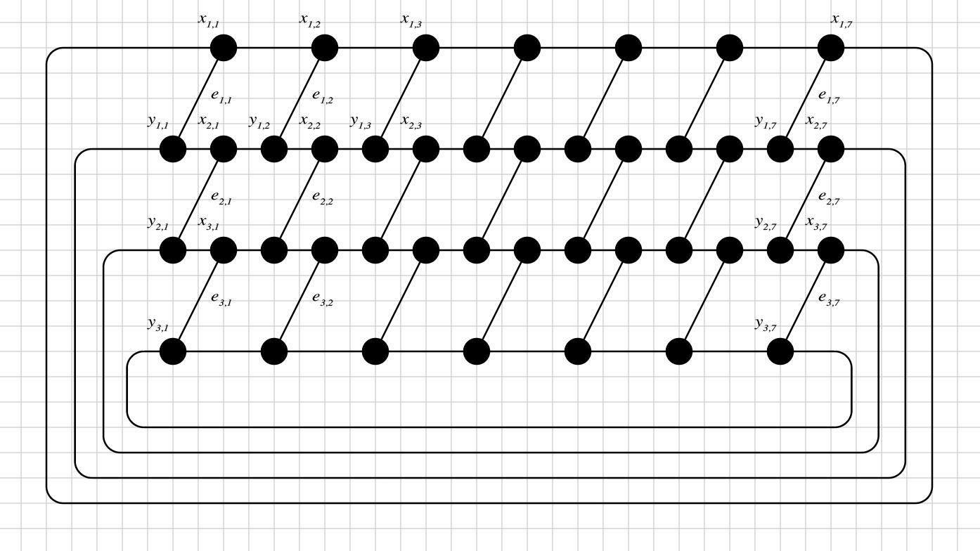
Figure 17: Graph $H_{f,k}$ when $k=4$ and $f(k)=2\cdot k-1=7$, with ${{E}\text{-}\mathsf{outerplanarity}}(H_{f,k})=4$, showing the naming conventions on edges and vertices (on some of them only, not to clutter the figure).

Definition 21 (Clusters, Holes in Clusters, Full Clusters).

A non-empty subset $X\subseteq\mathbf{V}(H_{f,k})$ is connected iff between any two vertices of $X$ there is a path. A cluster in graph $H_{f,k}$ is a non-empty connected subset $X\subseteq\mathbf{V}(H_{f,k})$.

Let $X,Y\subseteq\mathbf{V}(H_{f,k})$ be clusters in graph $H_{f,k}$. We say $Y$ is a hole in $X$, or that $X$ contains the hole $Y$, iff all of the following conditions are satisfied:

1. $X\cap Y=\varnothing$, i.e., $X$ and $Y$ are disjoint.

2. ${\partial}_{\,}(X,Y)\neq\varnothing$, i.e., there are edges with one endpoint in $X$ and one endpoint in $Y$.

3. ${\partial}_{\,}\bigl{(}\mathbf{V}(H_{f,k})-(X\cup Y),Y\bigr{)}=\varnothing$, i.e., there is no edge with one endpoint in $\mathbf{V}(H_{f,k})-(X\cup Y)$ and one endpoint in $Y$.

We say a cluster $X\subseteq\mathbf{V}(H_{f,k})$ is full iff $X$ contains no holes. An example of a cluster $X$ with a hole $Y$ is shown in Figure 18, and a full cluster is $X\cup Y$. $\square$

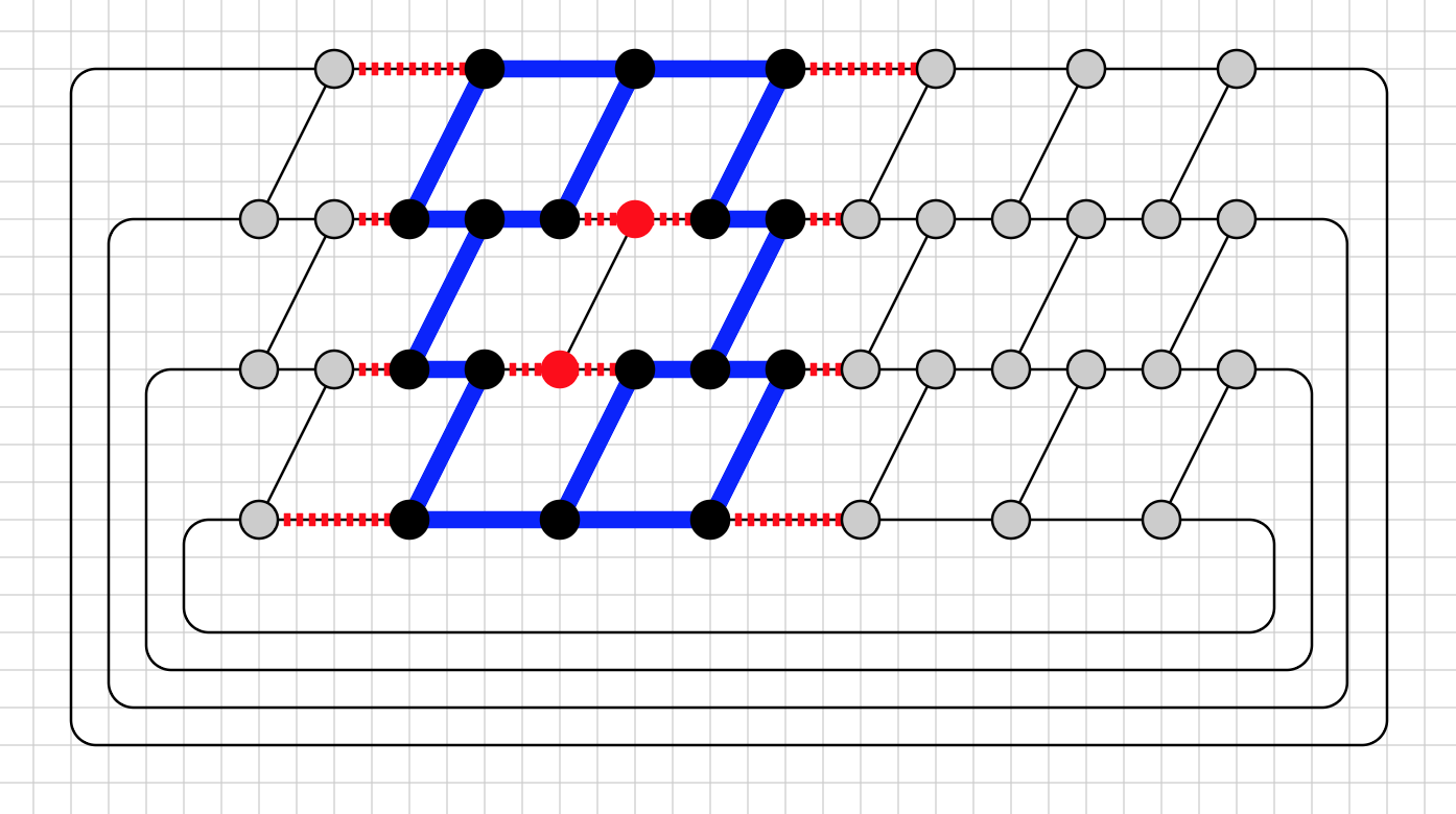
Figure 18: Example for Definition 21: Graph $H_{f,k}$ is the same as in Figure 17. The black vertices form a cluster $X$ in $H_{f,k}$, the red vertices form a hole $Y$ in $X$. The union $Z=X\cup Y$ is a full cluster.

Lemma 22.

Let $X\subseteq\mathbf{V}(H_{f,k})$ be a cluster in $H_{f,k}$. If $X$ contains holes, then there is a cluster $Z\subseteq\mathbf{V}(H_{f,k})$ without holes such that:

1. $\overline{\partial}_{\,}\bigl{(}Z\bigr{)}\leqslant\overline{\partial}_{\,}\bigl{(}X\bigr{)}\quad\text{and}\quad Z\supseteq X$.

2. For every full cluster $Z^{\prime}\supseteq X$, it holds that $|\,Z\,|\leqslant|\,Z^{\prime}\,|$.

In words, we can minimally augment ${X}$ and eliminate all the holes in it without increasing $\overline{\partial}_{\,}\bigl{(}X\bigr{)}$.

Proof.

Full clusters exist, with $\mathbf{V}(H_{f,k})$ being the largest full cluster. The desired $Z$ in the lemma statement is the smallest full cluster such that $Z\supseteq X$. It is straightforward to see that $\overline{\partial}_{\,}\bigl{(}X\bigr{)}\geqslant\overline{\partial}_{\,}\bigl{(}Z\bigr{)}$, since each hole in $X$ delete some vertices from $X$ and increases $\overline{\partial}_{\,}\bigl{(}X\bigr{)}$. ∎

The situation described in the statement of Lemma 22 is illustrated in Figure 18: For the full cluster $Z=X\cup Y$, we have $8=\overline{\partial}_{\,}\bigl{(}Z\bigr{)}\leqslant\overline{\partial}_{\,}\bigl{(}X\bigr{)}=12$.

Definition 23 (Frontiers of Full Clusters).

Other than its outermost face and its innermost face, every other face of $H_{f,k}$ is bounded by $5$ or $6$ edges. Call the outermost and innermost faces the large faces of $H_{f,k}$ (there are only two of them), and all the other faces the small faces of $H_{f,k}$ (there are $(k-1)\cdot f(k)$ of them).

Let $X\subseteq\mathbf{V}(H_{f,k})$ be a full cluster in graph $H_{f,k}$. Every face of $H_{f,k}$ is either inside or outside $X$. We say a face of $H_{f,k}$ is inside (resp. outside) $X$ iff all of the vertices (resp. one or more of the vertices) on the bounding edges of the face are in $X$ (resp. not in $X$). The frontier of $X$ is a set of edges defined as follows:

$$\text{\em frontier}(X)\triangleq\ \{\,e\in\mathbf{E}(H_{f,k})\;|\;\text{$e=\overline{x\ y}$ \ \ bounds a face outside $X$ and $\{x,y\}\subseteq X$}\,\}.$$

Note that if $e\in\text{\em frontier}(X)$, it does not necessarily follow that $e$ bounds a face inside $X$, even though the two endpoints of $e$ are in $X$; this is illustrated in Figure 19. And if $X$ is a face of $H_{f,k}$, large or small, then $\text{\em frontier}(X)$ coincides with the boundary of $X$. $\square$

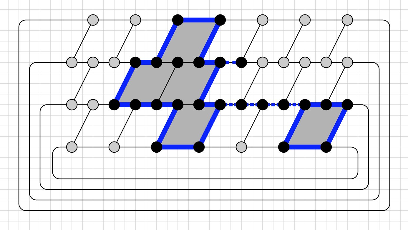
Figure 19: Example for Definitions 23 and 25: Graph $H_{f,k}$ is the same as in Figure 17. The black vertices form a full cluster $X$ in $H_{f,k}$. The faces in light gray are inside $X$; all the other faces are outside $X$. The edges in boldface form $\text{\em frontier}(X)$; not all edges in $\text{\em frontier}(X)$ bound a face inside $X$ (the dashed boldface edges) .

Lemma 24.

If $X\subseteq\mathbf{V}(H_{f,k})$ be a full cluster in $H_{f,k}$, then the set of vertices $\mathbf{V}\big{(}\text{\em frontier}(X)\big{)}$ forms a cluster, i.e., it is a non-empty connected subset of $\mathbf{V}(H_{f,k})$.

It is worth noting that, unless the vertices of the outermost cycle $C_{0}$ and/or the vertices of the innermost cycle $C_{k-1}$ are all in $X$, the vertices in $\mathbf{V}\big{(}\text{\em frontier}(X)\big{)}$ form a connected cactus.

Proof.

Straightforward from the definition. Details omitted. ∎

Definition 25 (Cut Edges, Dangling Edges, and Regular Clusters).

Let $X\subseteq\mathbf{V}(H_{f,k})$ be a full cluster in graph $H_{f,k}$, and consider $\text{\em frontier}(X)$. If $e\in\text{\em frontier}(X)$ does not bound a face inside $X$, then $e$ is one of two kinds:

• $e$ is a cut edge of $\text{\em frontier}(X)$,

• $e$ is a dangling edge of $\text{\em frontier}(X)$.

If the deletion of $e\in\text{\em frontier}(X)$ disconnects $\text{\em frontier}(X)$ into two components, then $e$ is a cut edge; otherwise, $e$ is a dangling edge. See Figure 19 for an illustration: it shows one dangling edge and three cut edges.

If $X$ is a full cluster and $\text{\em frontier}(X)$ contains no cut edges and no danling edges, then we say $X$ is a regular cluster; this is illustrated in Figure 20. Observe that a regular cluster is constructed from ‘piling on top of each other’ $5$-edge faces and $6$-edge faces. The $5$-edge faces are those adjacent to the outer face (bounded by $C_{0}$) and the innermost face (bounded by $C_{k-1}$). $\square$

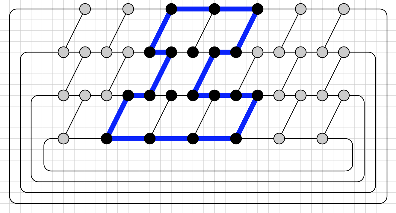
Figure 20: Example for Definition 25: Graph $H_{f,k}$ is the same as in Figure 17. The black vertices form a regular (full) cluster $X$ in $H_{f,k}$. There are no dangling edges and no cut edges in $\text{\em frontier}(X)$ .

Lemma 26.

Let $X\subseteq\mathbf{V}(H_{f,k})$ be a full cluster with $|\,X\,|\geqslant 3$. If $\text{\em frontier}(X)$ contains cut edges and/or dangling edges, then there is a regular cluster $Z\subseteq\mathbf{V}(H_{f,k})$ such that:

1. $\overline{\partial}_{\,}\bigl{(}Z\bigr{)}\leqslant\overline{\partial}_{\,}\bigl{(}X\bigr{)}\quad\text{and}\quad|\,Z\,|\geqslant|\,X\,|$.

2. For every regular cluster $Y$ such that $|\,Y\,|\geqslant|\,X\,|$, it holds that $|\,Z\,|\leqslant|\,Y\,|$.

In words, we can minimally augment the size $|\,X\,|$ and eliminate all cut edges and dangling edges from $\text{\em frontier}(X)$ without incrasing $\overline{\partial}_{\,}\bigl{(}X\bigr{)}$.

Proof.

The proof is an exhaustive case analysis. We proceed repeatedly to eliminate cut edges and dangling edges, one by one. There is no loss of generality in assuming that $X$ satisfies one of two conditions (or both):

1. $X\cap\mathbf{V}(C_{0})\neq\varnothing$ and $X\cap\mathbf{V}(C_{1})\neq\varnothing$,

2. $X\cap\mathbf{V}(C_{k-2})\neq\varnothing$ and $X\cap\mathbf{V}(C_{k-1})\neq\varnothing$.

In words, $X$ overlaps with the two outermost cycles (condition 1) and/or the two innermost cycles of $H_{f,k}$ (condition 2).

Consider a particular $e_{0}\in\text{\em frontier}(X)$ which is a cut edge or a dangling edge. Keep in mind that the two large faces of $H_{f,k}$ do not have a common boundary, that every small face of $H_{f,k}$ is bounded by $5$ or $6$ edges, and that every edge bounds exactly two faces.

Because $e_{0}\in\text{\em frontier}(X)$, there is a small face $F$ of $H_{f,k}$ outside $X$ which is bounded by $e_{0}$. Because $\text{\em frontier}(X)$ is connected, we can choose the face $F$ to be bounded by at least two edges of $\text{\em frontier}(X)$, say $e_{1}$ in addition to $e_{0}$. Let the set of edges bounding the small face $F$ be $\{e_{0},e_{1},e_{2},e_{3},e_{4}\}$ or $\{e_{0},e_{1},e_{2},e_{3},e_{4},e_{5}\}$.

In all cases satisfying one of the two following conditions:

• $F$ is bounded by $5$ edges, with at least two of them $\{e_{0},e_{1}\}\subseteq\text{\em frontier}(X)$,

• $F$ is bounded by $6$ edges, with at least three of them $\{e_{0},e_{1},e_{2}\}\subseteq\text{\em frontier}(X)$,

it is straightforward to add all the vertices of $\mathbf{V}(F)$ to $X$, thus increasing $|\,X\,|$ and making $F$ a face inside $X$, without increasing $\overline{\partial}_{\,}\bigl{(}X\bigr{)}$. All details of this straighforward case analysis are omitted.

The remaining cases satisfy the following condition:

• $F$ is bounded by $6$ edges, with exactly two of them $\{e_{0},e_{1}\}\subseteq\text{\em frontier}(X)$.

Because $F$ is bounded by $6$ edges, $F$ is not adjacent to the outer face (bounded by cycle $C_{0}$) nor to the innermost face (bounded by cycle $C_{k-1}$).

We eliminate cut edges of $\text{\em frontier}(X)$ first, by starting from cut edges of lowest level (those that are closest to cycle $C_{0}$), and we then proceed inward until we reach cut edges of highest level (closest to cycle $C_{k-1}$). In this order, it is easy to see that we only need to eliminate cut edges that satisfy condition 3 of condition 4 above.

We are left with the case when there are only dangling edges and condition $5$ is satisfied. Let therefore $e_{0}$ be a dangling edge of $\text{\em frontier}(X)$, which implies that $F$ is a $6$-edge face outside $X$ which shares $e_{1}$ as a bounding edge with another face inside $X$.

Let $e_{0}=\overline{v_{0}\ v_{1}}$ and $e_{1}=\overline{v_{1}\ v_{2}}$. Let $Y=X-\{v_{0}\}$, so that $\overline{\partial}_{\,}\bigl{(}Y\bigr{)}=\overline{\partial}_{\,}\bigl{(}X\bigr{)}-1$ and $|\,Y\,|=|\,X\,|-1$. Then $Y$ is a full cluster, such that $\text{\em frontier}(Y)$ contains no cut edges and one dangling edge less than $\text{\em frontier}(X)$. The desired full cluster $Z$ in the conclusion of the lemma is obtained by appropriately adding two or more vertices to $Y$ and by increasing $\overline{\partial}_{\,}\bigl{(}Y\bigr{)}$ by at most $1$.

Cluster $Y$ satisfies condition 1 or condition 2. Assume $Y$ satisfies condition 1. This implies there is a face $F^{\prime}$ with $5$ bounding edges, say $\{e^{\prime}_{0},e^{\prime}_{1},e^{\prime}_{2},e^{\prime}_{3},e^{\prime}_{4}\}$, such that edge $e^{\prime}_{0}$ is an ICE in $\text{\em frontier}(Y)$, edge $e^{\prime}_{1}$ is an edge of $C_{0}$ and also in $\text{\em frontier}(Y)$, edge $e^{\prime}_{2}$ is an ICE which may or may not be in $\text{\em frontier}(Y)$, and $\{e^{\prime}_{3},e^{\prime}_{4}\}$ are consecutive edges of cycle $C_{1}$ which may or may not be in $\text{\em frontier}(Y)$. It is now easy to see that we can add two (or more) vertices to $Y$ such that: (i) $\overline{\partial}_{\,}\bigl{(}Y\bigr{)}$ is increased by at most $1$ and (ii) no cut edge and dangling edge are added to $\text{\em frontier}(Y)$. The resulting cluster is the desired $Z$. ∎

Definition 27 ($\prec$-Sequences).

A maximal $\prec^{r}$-sequence $S$ of ICE’s in the graph $H_{f,k}$ is a sequence of the form:

$$S\ \triangleq\ e_{1,j}\ \prec^{r}\ e_{2,j}\ \prec^{r}\ \cdots\ \prec^{r}\ e_{k-1,j}$$

where $j\in\{1,\ldots,f(k)\}$. A maximal $\prec^{\ell}$-sequence $S$ of ICE’s in the graph $H_{f,k}$ is a sequence of the form:

$$S\ \triangleq\ e_{1,j_{1}}\ \prec^{\ell}\ e_{2,j_{2}}\ \prec^{\ell}\ \cdots\ \prec^{\ell}\ e_{k-1,j_{k-1}}$$

where $j_{1}\in\{1,\ldots,f(k)\}$ and:

$$j_{2}\ =\ 1+\big{(}(j_{1}-2)\!\!\!\mod f(k)\big{)},$$

$$j_{3} = 1+\big{(}(j_{1}-3)\!\!\!\mod f(k)\big{)},$$

$$\cdots$$

$$j_{k-1} = 1+\big{(}(j_{1}-k+1)\!\!\!\mod f(k)\big{)}.$$

A maximal $\prec$-sequence $S$ of ICE’s in the graph $H_{f,k}$ is a sequence of the form:

$$S\ \triangleq\ e_{1,j_{1}}\ \prec^{?}\ e_{2,j_{2}}\ \prec^{?}\ \cdots\ \prec^{?}\ e_{k-1,j_{k-1}}$$

where every pair $e_{p,j_{p}}\prec^{?}e_{p+1,j_{p+1}}$ in the sequence, with $1\leqslant p\leqslant k-1$, is:

$$\text{either}\quad e_{p,j_{p}}\ \prec^{r}\ e_{p+1,j_{p+1}}\quad\text{or}\quad e_{p,j_{p}}\ \prec^{\ell}\ e_{p+1,j_{p+1}},$$

i.e., in a maximal $\prec$-sequence it does not matter whether $e_{p+1,j_{p+1}}$ is a clockwise successor or counter-clockwise successor of $e_{p,j_{p}}$, as we traverse the sequence from the outermost cycle to the innermost cycle.

For graph $H_{f,k}$ with $k=4$ and $f(k)=8$, there are four possible shapes of maximal $\prec$-sequences; these are shown in boldface in Figure 21, with interleaving cycle edges inserted in dashed boldface.

Figure 21: Four possible shapes of maximal $\prec$-sequences in graph $H_{f,k}$ when $k=4$ and $f(k)=2\cdot k=8$ (slightly different from the graph in Figure 17). The leftmost above is a maximal $\prec^{r}$-sequence, the rightmost is a maximal $\prec^{\ell}$-sequence, and the two in the middle are neither maximal $\prec^{r}$ nor maximal $\prec^{\ell}$.

A $\prec^{r}$-sequence is a subsequence of a maximal $\prec^{r}$-sequence, i.e., the former is obtained by omitting a prefix and/or a suffix from the latter.

Similarly, a $\prec^{\ell}$-sequence is a subsequence of a maximal $\prec^{\ell}$-sequence, and a $\prec$-sequence is a subsequence of a maximal $\prec$-sequence. $\square$

Definition 28 (Strongly Regular Clusters).

Let $X\subseteq\mathbf{V}(H_{f,k})$ be a regular cluster with $|\,X\,|\geqslant 3$. We say $X$ is a strongly regular cluster bounded by the outermost cycle $C_{0}$ iff $\text{\em frontier}(X)$ can be partitioned into $4$ disjoint subsets:

• a subsequence of $n$ consecutive edges in $C_{0}$,

• a prefix of $p$ ICE’s in a maximal $\prec^{r}$-sequence together with their $(p-1)$ intermediate cycle edges,

• a subsequence of $q$ consecutive edges in $C_{p}$,

• a prefix of $p$ ICE’s in a maximal $\prec^{\ell}$-sequence together with their $(p-1)$ intermediate cycle edges,

for some $n,p,q\geqslant 1$. Symmetrically, we say $X$ is a strongly regular cluster bounded by the innermost cycle $C_{k-1}$ iff $\text{\em frontier}(X)$ can be partitioned into $4$ disjoint subsets:

• a subsequence of $n$ consecutive edges in $C_{k-1}$,

• a suffix of $p$ ICE’s in a maximal $\prec^{r}$-sequence together with their $(p-1)$ intermediate cycle edges,

• a subsequence of $q$ consecutive edges in $C_{k-1-p}$,

• a suffix of $p$ ICE’s in a maximal $\prec^{\ell}$-sequence together with their $(p-1)$ intermediate cycle edges,

for some $n,p,q\geqslant 1$. We call $n$, $p$, and $q$ the parameters of the strongly regular cluster $X$, the values of which are not totally arbitrary, as stated in the next lemma; $p$ is the height of $X$, and $n$ and $q$ its bases. Figure 22 shows an example of a strongly regular cluster bounded by the outermost cycle $C_{0}$ and Figure 23 shows an example of a strongly regular cluster bounded by the innermost cycle $C_{k-1}$. $\square$

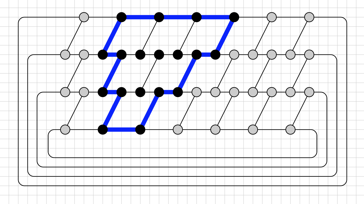
Figure 22: Example for Definition 28: Graph $H_{f,k}$ is the same as in Figure 17. The black vertices form a strongly regular cluster bounded by the outermost cycle $C_{0}$ .

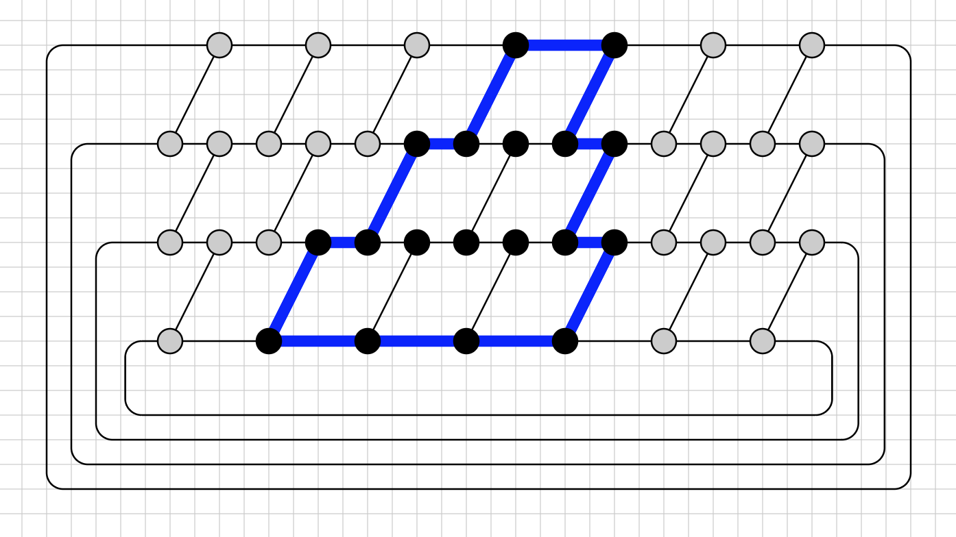
Figure 23: Example for Definition 28: Graph $H_{f,k}$ is the same as in Figure 17. The black vertices form a strongly regular cluster bounded by the innermost cycle, which is here $C_{3}$ .

Lemma 29.

If $X$ is a strongly regular cluster in $H_{f,k}$ with parameters $n$, $p$, and $q$, then:

1. $1\leqslant n\leqslant f(k)-1$ and $1\leqslant p\leqslant k-1$.

2. If $p<k-1$, then $q=2i$ for some $1\leqslant i\leqslant f(k)-p$,
   $p+(q/2)=n+1$,   $\overline{\partial}_{\,}\bigl{(}X\bigr{)}=2(p+1)+(q/2)$,  and $|\,X\,|=p^{2}+pq+p+(q/2)$.

3. If $p=k-1$, then $q=i$ for some $1\leqslant i\leqslant f(k)-p$,
   $p+q=n+1$,   $\overline{\partial}_{\,}\bigl{(}X\bigr{)}=2k$, and  $|\,X\,|=p^{2}+2pq+p$.

Proof.

Let $X$ be a strongly regular cluster bounded by the outermost cycle $C_{0}$. (The argument applies again symmetrically if $X$ is bounded by the innermost cycle $C_{k-1}$.)

For part 1, note that $n$ is restricted to be at most $f(k)-1$, it cannot be $f(k)$, because Definition 28 requires that the two bounding $\prec$-sequences be disjoint. Parts 2 and 3 follow from straightforward calculations (all details omitted). ∎

Lemma 30.

Let $X\subseteq\mathbf{V}(H_{f,k})$ be a regular cluster with $f(k)\gg k$. Let $N=|\,\mathbf{V}(H_{f,k})\,|$, the total number of vertices in $H_{f,k}$. If $|\,X\,|<N/2$ and $\overline{\partial}_{\,}\bigl{(}X\bigr{)}\leqslant 2k-1$, then there is a strongly regular cluster $Z\subseteq\mathbf{V}(H_{f,k})$ such that:

$$\overline{\partial}_{\,}\bigl{(}Z\bigr{)}\leqslant\overline{\partial}_{\,}\bigl{(}X\bigr{)}\quad\text{and}\quad|\,X\,|\leqslant|\,Z\,|<N/2.$$

Proof.

There is no loss of generality in assuming that $X$ satisfies condition 1 or condition 2 in the proof of Lemma 26. Since $\overline{\partial}_{\,}\bigl{(}X\bigr{)}\leqslant 2k-1$, it is only one of these two conditions that $X$ can satisfy, not both. We assume that $X$ satisfies condition 2 and thus view that $X$ has one or more consecutive $5$-edge faces at the bottom (all adjacent to the innermost face), on top of which there are $6$-edge faces, piled upward no higher than cycle $C_{1}$ in order not to violate the restriction $\overline{\partial}_{\,}\bigl{(}X\bigr{)}\leqslant 2k-1$. Moreover, because $|\,X\,|<N/2$ and $\overline{\partial}_{\,}\bigl{(}X\bigr{)}\leqslant 2k-1$, not all the vertices of the innermost cycle $C_{k-1}$ are in $X$, and because $X$ is full, there are paths connecting vertices in $C_{0}$ and $C_{k-1}$ whose vertices are all not in $X$.

Let $h\geqslant 1$ be the height of $X$, which is necessarily $\leqslant k-2$, otherwise we would have $\overline{\partial}_{\,}\bigl{(}X\bigr{)}\geqslant 2k$ contradicting the hypothesis. There are two kinds of edges connecting $X$ to $\big{(}\mathbf{V}(H_{f,k})-X\big{)}$ contributing to the total in $\overline{\partial}_{\,}\bigl{(}X\bigr{)}$: ICE’s and cycle edges. Consider all the ICE’s in the set ${{\partial}_{\,}(X)}$ at height $h$, say, these are $e_{1},e_{2},\ldots,e_{r}$ for some $r\geqslant 1$. These ICE’s are not necessarily consecutive, as there may be “dips” along $\text{\em frontier}(X)$.

The construction of the desired cluster $Z$ in the lemma conclusion proceeds in two stages. First, we remove all the “dips” between the top-level ICE’s $e_{1},e_{2},\ldots,e_{r}$ in ${{\partial}_{\,}(X)}$, to obtain an intermediate full cluster $X^{\prime}$ of the same height $h$ and where all the top-level ICE’s $e^{\prime}_{1},e^{\prime}_{2},\ldots,e^{\prime}_{s}$ in ${{\partial}_{\,}(X^{\prime})}$ are now consecutive and such that $\overline{\partial}_{\,}\bigl{(}X\bigr{)}\geqslant\overline{\partial}_{\,}\bigl{(}X^{\prime}\bigr{)}$ and $|\,X\,|\leqslant|\,X^{\prime}\,|$. By a ‘top-level ICE’ in ${{\partial}_{\,}(X)}$ we mean an ICE which is closest to the outermost cycle $C_{0}$. Note that

$$2k-1\ \geqslant\ \overline{\partial}_{\,}\bigl{(}X\bigr{)}\ \geqslant\ \overline{\partial}_{\,}\bigl{(}X^{\prime}\bigr{)}\ \geqslant 2(h+1)+s$$

In the last term, $2(h+1)$ is the number of cycle edges in ${{\partial}_{\,}(X^{\prime})}$ and $s$ is the number of ICE’s in ${{\partial}_{\,}(X^{\prime})}$ at height $h$. In general, there may be other ICE’s in ${{\partial}_{\,}(X^{\prime})}$ at heights lower than $h$.

Second, we obtain the desired regular cluster $Z$ by setting its parameters $p$ and $q$, as specified in Definition 28, and by Lemma 29, we do not need to also set its parameter $n$. We set $p=h$ and $q=2s$. By part 2 of Lemma 29, we have $\overline{\partial}_{\,}\bigl{(}Z\bigr{)}=2(h+1)+s$ and also $|\,Z\,|\leqslant|\,X^{\prime}\,|$. ∎

Lemma 31.

Let $X\subseteq\mathbf{V}(H_{f,k})$ be a strongly regular cluster with parameters $n$, $p$, and $q$, as specified in Definition 28. If $\overline{\partial}_{\,}\bigl{(}X\bigr{)}<2k$, then $|\,X\,|\leqslant\lceil(16k^{2}-32k+13)/12\rceil$.

Proof.

By part 3 of Lemma 29, if $\overline{\partial}_{\,}\bigl{(}X\bigr{)}<2k$ and therefore $\overline{\partial}_{\,}\bigl{(}X\bigr{)}\neq 2k$, then $p\neq k-1$. Because $X$ is strongly regular, it follows that $p<k-1$, by part 1 of Lemma 29. Hence, by part 2 of Lemma 29, we have:

$$|\,X\,|\ =\ p^{2}+pq+p+(q/2)\quad\text{and}\quad\overline{\partial}_{\,}\bigl{(}X\bigr{)}\ =\ 2(p+1)+(q/2).$$

Let $c$ be a constant such that $\overline{\partial}_{\,}\bigl{(}X\bigr{)}=c$ which we keep fixed throughout the proof. Relative to $c$, we determine how to set the values of the parameters $p$ and $q$ in order to maximize $|\,X\,|$. We first express $p$ in terms of $q$ and $c$, namely, if $2(p+1)+(q/2)=c$ then:

$$p\ =\ \frac{2c-q-4}{4}$$

which we substitute in $|\,X\,|=p^{2}+pq+p+(q/2)$ to obtain a function $f_{c}(q)$ depending on $q$ as a variable and $c$ as a constant:

$$f_{c}(q)\ \triangleq\ \ p\cdot(p+q+1)+\frac{q}{2}$$

$$= \Big{(}\frac{2c-q-4}{4}\Big{)}\cdot\Big{(}\frac{2c-q-4}{4}+q+1\Big{)}+\frac{q}{2}$$

$$= \frac{(2c-q-4)\cdot(2c+3q)+8q}{16}$$

$$= -(3/16)q^{2}+(1/4)(c-1)q+(1/4)(c^{2}-2c)$$

where the last expression is obtained from the preceding one by straightforward calculations. In the argument to follow, even though possible values of $c=2(p+1)+(q/2)$ are integers $\geqslant 5$, we deal with $q$ and $c$ as real numbers and we use the derivative of $f_{c}(q)$ relative to $q$ as such.

The function of $f_{c}(q)$ defines a parabola which is maximized at its vertex, i.e., at the value of $q$ for which the derivative:

$$f^{\prime}_{c}(q)\ \triangleq\ \frac{\text{d}f}{\text{d}q}=-(6/16)q+(1/4)(c-1)$$

is zero. Hence, $f_{c}(q)$ as a function over the reals is maximized at $\hat{q}$ given by:

$$\hat{q}\triangleq(2/3)(c-1).$$

After substituting $\hat{q}$ in $f_{c}(q)$ and carrying out straightforward calculations, we obtain:

$$f_{c}(\hat{q})\ =\ \frac{4c^{2}-8c+1}{12}$$

It is easily checked that $f_{c}(\hat{q})$ is monotonically increasing for all $c\geqslant 1$. By the lemma hypothesis, $c$ cannot exceed $2k-1\geqslant 1$. Substituting $2k-1$ for $c$ in $f_{c}(\hat{q})$, we obtain after simple calculations:

$$f_{2k-1}(\hat{q})\ =\ \frac{16k^{2}-32k+13}{12}.$$

We conclude that $|\,X\,|$ is an integer which cannot exceed the real number $(16k^{2}-32k+13)/12$. ∎

In the graph $H_{f,k}$ there are $k$ concentric cycles, such that two consecutive cycles are connected by $f(k)$ ICE’s. There is therefore a total of $(k-1)\cdot f(k)$ ICE’s in $H_{f,k}$, and since each ICE contributes two vertices, a total of $2(k-1)\cdot f(k)$ vertices. Hence, $|\,\mathbf{V}(H_{f,k})\,|=2(k-1)\cdot f(k)$.

Lemma 32.

Consider the family ${{\cal H}}_{f}=\{H_{f,k}\}$ where $k\geqslant 2$ and $f$ is any function such that the inequality:

$$\ 2(k-1)\cdot f(k)\ >\ 4\cdot\Big{(}\frac{16k^{2}-32k+13}{12}\Big{)}=\frac{16k^{2}-32k+13}{3}$$

is satisfied. Given any $H_{f,k}\in{{\cal H}}_{f}$ there is no binary reassembling ${\cal B}$ of $H_{f,k}$ such that $\alpha(H_{f,k},{\cal B})<2k$.

Proof.

If ${\cal B}$ is a binary reassembling of $H_{f,k}$ such that $\alpha(H_{f,k},{\cal B})<2k$, then for every node/cluster $X\in{\cal B}$ it holds that $\overline{\partial}_{\,}\bigl{(}X\bigr{)}<2k$. Let $N=|\,\mathbf{V}(H_{f,k})\,|$. To prove that no such ${\cal B}$ can exist, it suffices to show that for every cluster $X\in{\cal B}$, it must be that $|\,X\,|<N/2$, i.e., $X$ contains fewer than half the vertices of $H_{f,k}$, contradicting that ${\cal B}$ is a binary reassembling of $H_{f,k}$.

Given any two disjoint clusters $X_{1},X_{2}\in{\cal B}$ such that $\overline{\partial}_{\,}\bigl{(}X_{i}\bigr{)}<2k$ and $|\,X_{i}\,|<N/2$, with $i=1,2$, we show that if $\overline{\partial}_{\,}\bigl{(}X_{1}\cup X_{2}\bigr{)}<2k$, then again $|\,X_{1}\cup X_{2}\,|<N/2$. By Lemma 31, every strongly regular cluster $X$ with $\overline{\partial}_{\,}\bigl{(}X\bigr{)}<2k$ cannot include more than:

$$\frac{16k^{2}-32k+13}{12}$$

vertices. Hence, by Lemmas 22, 24, 26, 29, and 30, any cluster $X$, strongly regular or not, with $|\,X\,|<N/2$ and $\overline{\partial}_{\,}\bigl{(}X\bigr{)}<2k$ cannot include more than $(16k^{2}-32k+13)/12$ vertices. Hence,

$$|\,X_{1}\cup X_{2}\,|\ <\ \frac{16k^{2}-32k+13}{6}\ <\ \frac{N}{2}$$

The desired conclusion follows. ∎

Remark 33.

The inequality in the hypothesis of Lemma 32 can be simplified as follows. First, observe that:

$$(k-1)\cdot(16k-13)=16k^{2}-29k+13>16k^{2}-32k+13$$

for all $k\geqslant 2$. Hence, if $f$ satisfies the inequality:

$$\ 2(k-1)\cdot f(k)\ >\ \frac{(k-1)\cdot(16k-13)}{3}>\frac{16k^{2}-32k+13}{3}$$

then the hypothesis of Lemma 32 is satisfied. Hence, it suffices to require that $f$ is any number-theoretic function such that $f(k)>(16k-13)/6$. $\square$

Lemma 34.

For every graph $H_{f,k}\in{{\cal H}}_{f}$ where $f$ is any monotonically increasing or constant function $\geqslant 3$, algorithm $\mathsf{KS}$ on input $H_{f,k}$ returns a binary reassembling ${\cal B}=\mathsf{KS}(H_{f,k})$ such that $\alpha(H_{f,k},{\cal B})=2k$.

Proof.

The function $f$ plays no role in this proof. Assuming that $f(k)\geqslant 3$ for all $k$, it is easy to see that the binary reassembling ${\cal B}=\mathsf{KS}(H_{f,k})$ returned by algorithm $\mathsf{KS}$ is such that $\alpha(H_{f,k},{\cal B})=2k$. ∎

Theorem 35 (Optimality of Algorithm $\mathsf{KS}$).

For every graph in the family ${{\cal H}}_{f}$ where $f(k)>(16k-13)/6$, algorithm $\mathsf{KS}$ is an $\alpha$-optimal reassembling algorithm.

Proof.

Immediate consequence of Lemma 32, Remark 33, and Lemma 34. ∎

For the preceding theorem to hold, the number of ICE’s must increase as the edge-outerplanarity $k$ increases – this is the “density condition” mentioned in the opening paragraph of Section 5 – otherwise our algorithm $\mathsf{KS}$ is not an $\alpha$-optimal reassembling algorithm as we explain next.

We define a family of $3$-regular plane graphs, called ${{\cal G}}_{\ell}$ where $\ell\geqslant 3$, which exhibits a low “density of ICT’s” (or “inter-cycle density”) in the sense that their number is bounded by $\ell$ at every level. For every graph $G\in{{\cal G}}_{\ell}$:

• there is no restriction on $n=|\,\mathbf{V}(G)\,|$ or $k={{E}\text{-}\mathsf{outerplanarity}}(G)$, and both can be unboundedly large,

• at every level of $G$, the number of ICT’s is $\leqslant\ell$.

The second bullet point formalizes what we mean by low “inter-cycle density”. For the definition of level in $3$-regular plane graphs, review Definition 7.

It is possible to show (not in this report) that there is linear-time reassembling algorithm which, given an arbitrary $G\in{{\cal G}}_{\ell}$, returns an $\alpha$-optimal reassembling $(G,{\cal B})$ such that $\alpha(G,{\cal B})\in{\cal O}(\ell)$. A consequence of this fact is that our algorithm $\mathsf{KS}$ is not $\alpha$-optimal for the family ${{\cal G}}_{\ell}$. In the next proposition, we prove a particular case: We consider the family ${{\cal H}}_{f}$ as defined in the opening paragraphs of Section 5, where every ICT is an inter-cycle edge (ICE), and choose a particular function $f$, called $\bar{f}$, which makes ${{\cal H}}_{\bar{f}}$ a proper subclass of ${{\cal G}}_{\ell}$ for sufficiently large $\ell$, i.e., ${{\cal H}}_{\bar{f}}\subsetneq{{\cal G}}_{\ell}$. The $\bar{f}$ in question is a constant function, specifically here: $\bar{f}(k)=c$ for some constant $c\geqslant 3$ which makes ${{\cal H}}_{\bar{f}}\subsetneq{{\cal G}}_{c}$. Thus, for every $H_{\bar{f},k}\in{{\cal H}}_{\bar{f}}$, the number of inter-cycle one-edge trees at every level of $H_{\bar{f},k}$ is $c$ and independent of $k$

Proposition 36.

Let $c$ be a constant $\geqslant 3$. There is linear-time $\alpha$-optimal reassembling algorithm ${\cal A}$ for the family ${{\cal H}}_{\bar{f}}$ where $\bar{f}(k)=c$. Specifically, given an arbitrary $H_{\bar{f},k}\in{{\cal H}}_{\bar{f}}$, algorithm ${\cal A}$ returns in time ${\cal O}(|\,\mathbf{V}(H_{\bar{f},k})\,|)$ an $\alpha$-optimal reassembling ${\cal B}$ of $H_{\bar{f},k}$ such that $\alpha(H_{\bar{f},k},{\cal B})=c+2$.

By contrast, given an arbitrary $H_{\bar{f},k}\in{{\cal H}}_{\bar{f}}$ as input, algorithm $\mathsf{KS}$ returns a reassembling ${\cal B}$ of $G$ such that $\alpha(H_{\bar{f},k},{\cal B})=2\cdot{{E}\text{-}\mathsf{outerplanarity}}(H_{\bar{f},k})=2k$. Hence, $\mathsf{KS}$ is not an $\alpha$-optimal reassembling algorithm for the family ${{\cal H}}_{\bar{f}}$.

Proof Sketch. We restrict the proof to the case $c=3$, so that $\bar{f}(k)=3$ for every $k={{E}\text{-}\mathsf{outerplanarity}}(H_{\bar{f},k})$; the proof is easily generalized for any $c\geqslant 3$. With this restriction, there is a total of $6k^{\prime}$ vertices in $H_{\bar{f},k}\in{{\cal H}}_{\bar{f}}$ where we pose $k^{\prime}=k-1$. Let $\mathbf{V}(H_{\bar{f},k})=\{a_{1},a_{2},\ldots,a_{6k^{\prime}}\}$, with “$a_{1}\;a_{2}\;a_{3}$” be the clockwise sequence of vertices of the innermost cycle $L_{k-1}$. (We use the naming conventions for the nested cycles introduced in Definition 4.) Continuing inside-out, “$a_{4}\ \cdots\ a_{9}$” is the clockwise sequence of vertices of the next cycle $L_{k-2}$, etc., and “$a_{6k^{\prime}-2}\;a_{6k^{\prime}-1}\;a_{6k^{\prime}}$” is the clockwise sequence of vertices of the outermost cycle $L_{0}$. See the top of Figure 24 for the case $k=5$.

It is easy to check that an $\alpha$-optimal reassembling of $H_{\bar{f},k}$ (not the only one) proceeds as follows:

$$\bigl{\{}\bigl{\{}\bigl{\{}\bigl{\{}\ldots\{\{\{\{\{\{\{\{a_{1},a_{2}\}^{4},a_{3}\}^{3},a_{4}\}^{4},a_{5}\}^{5},a_{6}\}^{4},a_{7}\}^{5},a_{8}\}^{4},a_{9}\}^{3}\ldots a_{6k^{\prime}-3}\bigr{\}}^{3},a_{6k^{\prime}-2}\bigr{\}}^{4},a_{6k^{\prime}-1}\bigr{\}}^{3},a_{6k^{\prime}}\bigr{\}}^{0}$$

where the superscript of every cluster is its edge-boundary degree. For example, the contraction of the edge $\overline{a_{1}\;a_{2}}$ produces a super vertex/cluster of degree $4$, i.e., $\overline{\partial}_{\,}\bigl{(}\{a_{1},a_{2}\}\bigr{)}=4$, and then the contraction of the edge $\overline{\overline{a_{1}\;a_{2}}\;a_{3}}$ produces a super vertex/cluster of degree $3$, i.e., $\overline{\partial}_{\,}\bigl{(}\{a_{1},a_{2},a_{3}\}\bigr{)}=3$, etc. The first three contractions of this reassembling are depicted in the bottom of Figure 24 for the case $k=5$.

The resulting reassembling tree ${\cal B}$, as just described, is such that $\alpha(H_{\bar{f},k},{\cal B})=5$, whereas algorithm $\mathsf{KS}$ on input $H_{\bar{f},k}$ returns a reassembling tree $\mathsf{KS}(H_{\bar{f},k})={{\cal B}}^{\prime}$ such that $\alpha(H_{\bar{f},k},{{\cal B}}^{\prime})=2k$. $\square$

Whereas algorithm $\mathsf{KS}$ proceeds in an ‘outside-in’ fashion (starting from the outermost cycles), the reassembling in the preceding proof proceeds ‘inside-out’ (starting from the innermost cycle). However, the order of the latter can be reversed to work ‘outside-in’ optimally too.

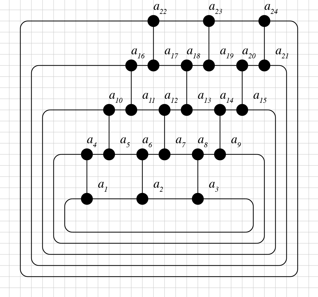
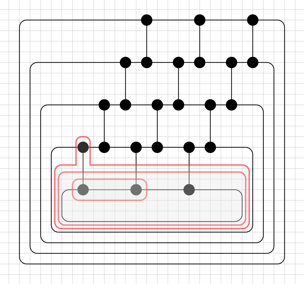
Figure 24: For Proposition 36: Graph $H_{\bar{f},k}$ when $k=4$ and $\bar{f}(k)=3$.
The lower figure depicts the first three contractions of an $\alpha$-optimal reassembling:
$\overline{a_{1}\;a_{2}}$,  $\overline{\overline{a_{1}\;a_{2}}\;a_{3}}$,  and $\overline{\overline{\overline{a_{1}\;a_{2}}\;a_{3}}\;a_{4}}$.

6 Conclusion

We developed a linear-time algorithm $\mathsf{KS}$ for the reassembling of $3$-regular plane graphs. Given such a graph $G$ as input, with ${{E}\text{-}\mathsf{outerplanarity}}(G)=k\geqslant 2$, algorithm $\mathsf{KS}$ returns a binary reassembling ${\cal B}=\mathsf{KS}(G)$ of $G$ such that $\alpha(G,{\cal B})=2k$.

In Section 4 we proved the correctness of algorithm $\mathsf{KS}$ and its time complexity, preceded by several examples illustrating the progression of $\mathsf{KS}$ on several graphs exhibiting different peculiarities (Section 4.5). In Section 5 we showed that our algorithm is optimal for the class of $3$-regular plane graphs that have a sufficiently high “inter-cycle density” which increases as the edge-outerplanarity increases (this informal description is made precise in Section 5).

6.1 Related Work

In Section 2.1 we spelled out the connection between graph carving and graph reassembling. The first of these two notions has been studied for many years. A number of results about graph carving are readily translated into results about graph reassembling. We mention two of the most salient.

Proposition 37.

There exists an algorithm which, given a plane graph $G$ (not necessarily $3$-regular) as input with $n$ vertices, returns in time ${\cal O}\bigl{(}n^{3}\bigr{)}$ a binary reassembling ${\cal B}$ of $\mathbf{V}(G)$ such that $(G,{\cal B})$ is $\alpha$-optimal.

Proof.

This is an immediate consequence of Proposition 1 in this report and Theorem 2.1 in [3]. ∎

The next proposition is about the existence of a fixed-parameter linear-time algorithm where the parameter-bound not to be exceeded is the $\alpha$-measure. This is to be contrasted with our algorithm $\mathsf{KS}$, which can be recast (not here) as a fixed-parameter linear-time algorithm where the parameter-bound not to be exceeded is the edge-outerplanarity. As usual, ‘linear time’ means ‘linear as a function of the number $n$ of vertices’.

Proposition 38.

Let $p\geqslant 1$ be fixed. There exists a linear-time algorithm that checks whether an input graph $G$ (not necessarily plane) has a binary reassembling ${\cal B}$ of its vertices $\mathbf{V}(G)$ such that $\alpha(G,{\cal B})\leqslant p$ and, if this is the case, the algorithm returns a reassembling ${\cal B}$ such that $(G,{\cal B})$ is $\alpha$-optimal.

Proof.

This is a straightforward consequence of Proposition 1 in this report and the main result in [15] (Theorem 1 and Theorem 2 in Section 6). ∎

We can also state, in reverse, implications from results on graph reassembling to results on graph carving, illustrated by the following proposition. Review the definitions related to graph carving in Section 2.1.

Proposition 39.

There exists a linear-time algorithm which, given an arbitrary $3$-regular plane graph $G$ as input with ${{E}\text{-}\mathsf{outerplanarity}}(G)=k\geqslant 2$, returns a routing tree $T$ for $G$ such that $0pt{G,T}\leqslant 2k$.

Note, in particular, the value of $0pt{G,T}$ in the returned routing tree $T$ is independent of $n=|\,\mathbf{V}(G)\,|$.

Moreover, for the family of graphs ${{\cal H}}_{f}$ defined at the beginning of Section 5, the bound $2k$ in Proposition 39 is an optimal carving width, by Theorem 35.

Proof.

Straightforward consequence of Proposition 1, Theorem 9, and Corollary 20, in this report. ∎

6.2 Future Research

One obvious task for the future is to extend our method for $3$-regular plane graphs to arbitrary plane graphs. However, short of such an extension (which seems to require a considerable effort to formulate with an equal loss in transparency), we know there is at least one important application, discussed next, for which there is no explicit need for extending our method beyond its current form. Other applications are yet to be identified.

Consider an application involving the computation of maximum flows in networks. We take a flow network to be a capacited directed graph $G$ with no self-loops and two distinguished vertices, a source vertex $s$ and a sink vertex $t$, which we identify by the quadruple $(G,c,s,t)$ where $c:\mathbf{E}(G)\to\mathbb{R}_{+}$ is the (non-negative) capacity function. A flow $f:\mathbf{E}(G)\to\mathbb{R}_{+}$ is feasible if $f(e)\leqslant c(e)$ for every $e\in\mathbf{E}(G)$ and $f$ satisfies the usual flow-conservation condition at every vertex $v\in\mathbf{V}(G)-\{s,t\}$. We write $|\,f\,|$ to denote the value of the flow $f$, which is the excess flow exiting $s$ or, equivalently, the excess flow entering $t$.

Given a network $(G,c,s,t)$, we can transform it into an equivalent $(G^{*},c^{*},s^{*},t^{*})$ in time ${\cal O}(n)$ where $n=|\,\mathbf{V}(G)\,|$ and every vertex $v\in\mathbf{V}(G^{*})$ has degree $=3$. Moreover, if $G$ is plane, then so is $G^{*}$ such that ${{E}\text{-}\mathsf{outerplanarity}}(G)={{E}\text{-}\mathsf{outerplanarity}}(G^{*})$. The crux of the transformation $(G,c,s,t)\mapsto(G^{*},c^{*},s^{*},t^{*})$ is an expansion of every $v\in\mathbf{V}(G^{*})$ of degree $\geqslant 4$; Figure 25 shows the expansion of a degree-$5$ vertex.

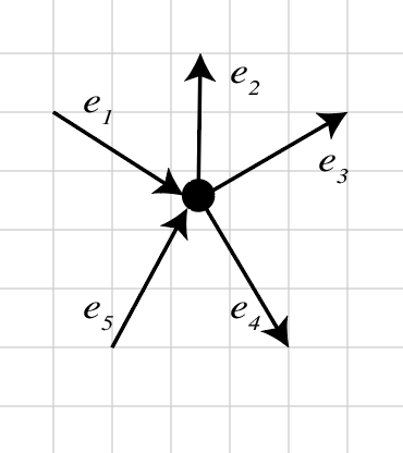
Figure 25: A vertex of degree $=5$ (on the left) which is transformed into a cycle (on the right),
with $5$ vertices each of degree $=3$ and the same incident edges $\{e_{1},e_{2},e_{3},e_{4},e_{5}\}$.

The details of the transformation $(G,c,s,t)\mapsto(G^{*},c^{*},s^{*},t^{*})$ will be in a separate report [9], which will also include a proof of the following result.

Proposition 40.

There is a fixed-parameter linear-time algorithm to compute max flow in planar flow networks $(G,c,s,t)$, where the parameter-bound not to be exceeded is $k={{E}\text{-}\mathsf{outerplanarity}}(G)$.

We conclude with a conjecture which, we believe, can be examined using the methodology developed in this paper. To make sense of the conjecture statement, review how we classify and define the level of inter-cycle trees (ICT’s) in Definition 4, Propositions 5 and 6, and the Remark. on page 4.3.

Conjecture 41.

There is a function $f:\mathbb{N}\to\mathbb{N}$ such that, for every $3$-regular plane graph $G$, if for every level $j\in\{0,\ldots,k-1\}$ where $k={{E}\text{-}\mathsf{outerplanarity}}(G)$ the number of level-$j$ ICT’s is $\geqslant f(k)$, then $\mathsf{KS}$ is an $\alpha$-optimal reassembling algorithm for $G$, i.e., $\mathsf{KS}$ returns a reassembling ${\cal B}=\mathsf{KS}(G)$ such that $\alpha(G,{\cal B})=2k$ is optimal. $\square$

If Conjecture 41 is true, it defines a larger class of $3$-regular plane graphs than Theorem 35 for which $\mathsf{KS}$ is an $\alpha$-optimal reassembling algorithm. (Theorem 35 is about $3$-regular plane graphs where every ICT is an ICE, an inter-cycle edge.)

A final open problem is: Characterize the class of all $3$-regular plane graphs for which $\mathsf{KS}$ is an $\alpha$-optimal reassembling algorithm.

Appendix A Appendix: Pseudocode of Algorithm $\mathsf{KS}$

Below is the pseudocode of algorithm $\mathsf{KS}$, of which the full Python code is an elaboration. The latter can be dowloaded from the website Graph Reassembling. The pseudocode is based on the description in Sections 4.1 4.2, 4.3, and 4.4. For easier cross-referencing, we use the following conventions in the pseudocode:

1. Lines in black blodface appear verbatim in the Python code; these are headings of function definitions.

2. Lines in black Roman characters, which do not start with a hash #, describe each an action that is implemented with several Python instructions; they are inserted as comments throughout the Python code in order to make the Python code more readable.

3. Lines in grey Roman characters, which start with a hash #, are inserted as comments in the Python code; they describe the state of the execution at the points where they are inserted.

4. Lines in red are related to the collapse operation, lines in green are related to the merge operation. We follow the same color convention in our examples in Section 4.5.

def pre-process():
    let the current E-outerplanarity level be 0

    # by marking edges at each E-outerplanarity layer one at a time
    # the trees and cycles can be differentiated
    initialize every vertex such that all vertices are unmarked
    while the graph has edges left unmarked
        starting at the upper leftmost unmarked vertex,
        traverse the graph by taking the next clockwise edge at each vertex encountered,
        marking each time a vertex is visited,
        until the traversal returns to the original vertex

        the edge of this particular E-outerplanarity are now
        defined to be all the edges traversed

        for all edges traversed
            if the edge was traversed once
                the edge is part of a cycle
            otherwise
                # the edge has been marked exactly twice
                the edge is part of a cycle

        for all vertices that have two incident cycle edges
            # the vertex will have exactly one incident tree edge
            if the tree edge is on the same E-outerplanarity as the vertex
                then it is an outward cycle vertex
            otherwise
                then it is an inward cycle vertex

        to determine the vertices of a particular cycle or tree
            begin a depth-first search at both endpoints of a tree or cycle edge
            and traverse every edge adjacent of the same type
            two cycles or two trees will never share the same vertex,
            so the depth-first search will traverse the entire tree or cycle and then end
            # the entire graph will be traversed once as a whole
            # all leaf vertices will be visited twice
            # while other vertices will be visited once

        increment the E-outerplanarity by 1

def process():
    at each E-outerplanarity level in the graph
        define a queue that holds trees to be collapsed and merged

    prepare_cycle(outermost cycle enclosing the whole graph)

    while any queue is not empty
        pop the oldest tree in the queue at the deepest E-outerplanarity level
        if the tree has not collapsed
            collapse the tree
        otherwise
            merge the tree

def collapse˙type˙a(tree):
    refer to the upper left most vertex of tree as v
    collapse_tree(tree,v)
    add tree to the queue for this layer so it merges as a type A tree

def collapse˙type˙b(v):
    refer to the tree v is part of as tree

    refer to the root of tree as u
    # note that u and v will never be the same vertex

    collapse_tree(tree,v)
    add tree to the queue for this layer so it merges as a type B tree


def merge˙type˙a(tree):
    refer to the cycle enclosing tree as the outer cycle
    refer to the super node that tree is part of as super

    if the outer cycle has no incident trees left uncollapsed
        merge_cycle(the outer cycle, super)
        return

    otherwise, if the outer cycle has a single incident tree left uncollapsed
        prep_incident_tree(the outer cycle, super)
        return

    find a vertex adjacent to tree on the outer cycle that
        is part of a tree on the same layer as tree
        and is not in the same super vertex as tree

    if that vertex does not exist
        # there is nothing to do until the outer cycle is ready to merge
        because the outer cycle is waiting on a tree that is not adjacent to this tree
        return

    refer to that vertex as the successor vertex
    refer to the tree that the successor vertex is part of as the successor tree

    if the successor tree is Type-B
        if the successor tree has merged
            # there is nothing to do because there is nowhere for us to merge
            that has not already merged
            return
        # the successor vertex will never be the root vertex of the successor tree
        merge super and the super node of which the successor vertex is a part

    otherwise, if the successor tree is Type-B or it has not collapsed yet
        merge super and the successor vertex
        if successor tree is ready to collapse
# the successor tree may be either type A or type B
            add the successor tree to the queue for this layer
            so it merges with the proper type

    otherwise,
        # the successor tree is a type A tree that has collapsed but not yet merged
        merge super and the super node of which the successor tree is a part

def merge˙type˙b(v):
    refer to the super node that v is part of as the super
    refer to the cycle v is a on as cycle
    refer to the clockwise successor of v on cycle as the successor vertex
    refer to the tree v is part of as tree

    marked v as collapsed as it was not marked as collapsed earlier

    if the successor vertex is an outer vertex
        if there is nothing stored with the successor vertex
            refer to the tree that the successor vertex is part of
            as the successor tree
            merge the super and the successor vertex
            if the successor tree is the only tree left on cycle uncollapsed
            and it is ready to collapse
                add the successor tree to the queue for this layer
                so it merges as a type B tree

        otherwise, if there are any trees on cycle left uncollapsed
            merge super and the super node of which the successor vertex is a part


        otherwise,
            # cycle has been entirely collapsed and is ready to merge
            merge_cycle(layer_states, layer, rs, c, super)

    otherwise
        merge super and the successor vertex
        if cycle has 0 or 1 incident trees left uncollapsed
        and it has not been prepared
            prep_cycle(cycle)

def merge˙cycle(cycle, super):
    refer to the cycle enclosing cycle as the outer cycle

    find the clockwise successor tree of this cycle on the layer of the outer cycle

    if there is such a tree
        merge super and the vertex closest to this cycle

    otherwise, if the outer cycle is the outermost cycle
        the graph has been fully collapsed and no more work is left

    otherwise, if the outer cycle has any incident trees left uncollapsed
        # it will have exactly one incident tree left uncollapsed
        prepare_incident_tree(the outer cycle, super)

    otherwise,
        # we must recurse upwards to continue
        merge_cycle(the outer cycle, super)

def prep˙incident˙tree(cycle, super):
    # there is exactly one tree uncollapsed incident to this cycle
    merge cycle and the root vertex of the incident tree on cycle
    if the incident tree is ready to collapse
        add the incident tree to the queue for this layer so it as a type B tree

def collapse˙tree(tree,x):
    refer to the vertex adjacent to x as v
    note that x will always be leaf vertex of tree

    if v is a leaf vertex of tree
        assign an index to x
        assign an index to v
        tree is a tree consisting of two vertices
        return the super vertex of x and v

    while v != x:
        if v is a leaf vertex
            assign an index to v
            set v to the predecessor of v
            continue

        refer to the left child of v as l
        refer to the right child of v as l

        if l does not have an index
            v is the predecessor of l
            set v to l
            continue

        if r does not have an index
            v is the predecessor of l
            set v to l
            continue

        note that at this point, l and r may be super vertices,
        but v is definitely not
        assign an index to v
        collapse l and v into a super vertex
        collapse the result with r and store it under v
        set v to the predecessor of v

    assign an index to x
    return the super vertex of x and v

References

- [1] Cedric Bentz. Disjoint paths in sparse graphs. Discrete Applied Mathematics, 157(17):3558–3568, 2009.
- [2] Azer Bestavros and Assaf Kfoury. A Domain-Specific Language for Incremental and Modular Design of Large-Scale Verifiably-Safe Flow Networks. In Proc. of IFIP Working Conference on Domain-Specific Languages (DSL 2011), EPTCS Volume 66, pages 24–47, Sept 2011.
- [3] Qian-Ping Gu and Hisao Tamaki. Optimal Branch-Decomposition of Planar Graphs in Time. ACM Transactions on Algorithms, 4(3), June 2008.
- [4] Dorit S. Hochbaum. Why Should Biconnected Components Be Identified First. Discrete Appl. Math., 42(2-3):203–210, April 1993.
- [5] John Hopcroft and Robert Tarjan. Algorithm 447: Efficient Algorithms for Graph Manipulation. Communications of the ACM, 16(6):372–378, June 1973.
- [6] Frank Kammer. Determining the Smallest Such That Is -Outerplanar. In Lars Arge, Michael Hoffmann, and Emo Welzl, editors, Proc. of 15th Annual European Symposium on Algorithms, ESA 2007, pages 359–370. LNCS 4698, Springer Verlag, September 2007.
- [7] Assaf Kfoury. The Denotational, Operational, and Static Semantics of a Domain-Specific Language for the Design of Flow Networks. In Proc. of SBLP 2011: Brazilian Symposium on Programming Languages, Sept 2011.
- [8] Assaf Kfoury. The Syntax and Semantics of a Domain-Specific Language for Flow-Network Design. Science of Computer Programming, 93(Part A):19–38, November 2014.
- [9] Assaf Kfoury. A Fixed-Parameter Linear-Time Algorithm for Maximum Flow in Planar Flow Networks. Uploaded to arxiv.org, July 2018.
- [10] Assaf Kfoury and Saber Mirzaei. Efficient Reassembling of Graphs, Part 1: The Linear Case. J. of Combinatorial Optimization, 33(3):1057–1089, April 2017.
- [11] Saber Mirzaei and Assaf Kfoury. Efficient Reassembling of Graphs, Part 2: The Balanced Case. CoRR, abs/1602.02863, 2016. preprint, http://arxiv.org/abs/1602.02863v1.
- [12] Maurizio Patrignani. Planarity Testing and Embedding. In Roberto Tamassia, editor, Hanbook of Graph Drawing and Visualization, pages 1–42. CRC Press, Baton Rouge, FL, 2013.
- [13] Paul D. Seymour and Robin Thomas. Call Routing and the Ratcatcher. Combinatorica, 14(2):217–241, 1994.
- [14] Nate Soule, Azer Bestavros, Assaf Kfoury, and Andrei Lapets. Safe Compositional Equation-based Modeling of Constrained Flow Networks. In Proc. of 4th Int’l Workshop on Equation-Based Object-Oriented Modeling Languages and Tools, Zürich, September 2011.
- [15] Dimitrios M. Thilikos, Maria J. Serna, and Hans L. Bodlaender. Constructive Linear-Time Algorithms for Small Cutwidth and Carving-Width. In Gerhard Goos, Juris Hartmanis, Jan van Leeuwen, D. T. Lee, and Shang-Hua Teng, editors, Algorithms and Computation: 11th International Conference, ISAAC 2000 Taipei, Taiwan, December 18–20, 2000 Proceedings, pages 192–203. Springer Berlin Heidelberg, Berlin, Heidelberg, 2000.