Phase reconstruction from amplitude spectrograms
based on von-Mises-distribution deep neural network

Abstract

This paper presents a deep neural network (DNN)-based phase reconstruction from amplitude spectrograms. In audio signal and speech processing, the amplitude spectrogram is often used for processing, and the corresponding phase spectrogram is reconstructed from the amplitude spectrogram on the basis of the Griffin-Lim method. However, the Griffin-Lim method causes unnatural artifacts in synthetic speech. Addressing this problem, we introduce the von-Mises-distribution DNN for phase reconstruction. The DNN is a generative model having the von Mises distribution that can model distributions of a periodic variable such as a phase, and the model parameters of the DNN are estimated on the basis of the maximum likelihood criterion. Furthermore, we propose a group-delay loss for DNN training to make the predicted group delay close to a natural group delay. The experimental results demonstrate that 1) the trained DNN can predict group delay accurately more than phases themselves, and 2) our phase reconstruction methods achieve better speech quality than the conventional Griffin-Lim method.

Index Terms—  speech analysis, phase reconstruction, deep neural network, von Mises distribution, group delay

1 Introduction

A variety of audio signal processing and machine learning-based methods, such as audio source separation and speech enhancement, involve processing the amplitude spectrogram obtained via short-term Fourier transform (STFT). Also, statistical parametric text-to-speech synthesis [1] is shifting from vocoder-based (source filter model-based) to STFT-based frameworks [2, 3, 4]. To produce synthetic speech, we require the corresponding phase spectrogram, but it is often unavailable. The Griffin-Lim method [5] is a well-known example that iteratively estimates of the phase spectrogram through STFT and inverse STFT while fixing the amplitude spectrogram. This signal-processing-based method has high portability without a priori training but causes unnatural artifacts in synthetic speech. Therefore, this paper proposes building a trainable phase reconstruction method using generative models.

A deep neural network (DNN) is a powerful generative model. There are two types of distributions: non-parametric [6, 7, 8, 9] and parametric ones. This paper addresses the latter. There are many types of the parametric approaches related to the Gaussian distribution, e.g., isotropic multivariate Gaussian [10] and temporal-delta-constrained Gaussian [11, 12] (a.k.a., trajectory DNN in statistical parametric speech synthesis). The loss function (e.g., mean squared error) for training DNNs is often derived to minimize the negative log-likelihood of the distribution. The straightforward way to predict a phase spectrogram from an amplitude spectrogram is to use these models. However, the Gaussian distribution is inappropriate for modeling distributions of a phase that is a periodic variable with a period of $2\pi$.

This paper proposes phase reconstruction from amplitude spectrograms based on the von-Mises-distribution DNN. The von Mises distribution is a probability distribution on the circle [13], which is suitable for modeling periodic variables. The von-Mises-distribution DNN is a generative model that has the von Mises distribution as a conditional probability distribution. The von-Mises-distribution shallow neural network was originally proposed by Nabney et al. [14], and this paper utilizes it for predicting the phase spectrogram from the amplitude spectrogram. The loss function for DNN training, named the phase loss (see Fig. 1), is defined by minimizing likelihoods of the von Mises distribution. Also, we propose another loss function named group-delay loss, which has a stronger connection to the amplitude spectrum [15]. The group-delay loss is used to make group delay of the predicted phase close to that of the target phase. Since the group delay and group-delay loss are differentiable by the phase, the DNN can be trained by a standard backpropagation algorithm. We conduct objective and subjective evaluations to evaluate the effectiveness of the proposed methods. The results demonstrate that 1) the trained DNN can predict group delay accurately more than phases themselves, and 2) our phase reconstruction method outperforms the conventional Griffin-Lim method in terms of quality of synthesized speech.

Fig. 1: Overview of proposed phase reconstruction method. This figure shows frame-by-frame phase prediction rather than multi-frame or sequence-wise prediction for clear illustration.

2 Griffin-Lim phase reconstruction

This section briefly describes the conventional Griffin-Lim method [5]. The Griffin-Lim method is a signal-processing-based iterative algorithm to reconstruct a phase spectrogram from the amplitude spectrogram. Let $\textrm{\boldmath$x$}=\left[\textrm{\boldmath$x$}_{1},\cdots,\textrm{\boldmath$x$}_{t},\cdots,\textrm{\boldmath$x$}_{T}\right]$ and $\textrm{\boldmath$y$}=\left[\textrm{\boldmath$y$}_{1},\cdots,\textrm{\boldmath$y$}_{t},\cdots,\textrm{\boldmath$y$}_{T}\right]$ be amplitude and phase spectrograms, respectively. $\textrm{\boldmath$x$}_{t}=\left[x_{t,0},\cdots,x_{t,f},\cdots,x_{t,F}\right]$ and $\textrm{\boldmath$y$}_{t}=\left[y_{t,0},\cdots,y_{t,f},\cdots,y_{t,F}\right]$ are the amplitude and phase at frame $t$, respectively. $f$ is the frequency index, and $F$ corresponds to the Nyquist frequency. Both $x_{t,f}$ and $y_{t,f}$ are real-valued variables, but only $y_{t,f}$ is a variable with a period of $2\pi$. The Griffin-Lim method randomly initializes $y$ first. 1) Then it takes inverse STFT to obtain a waveform from $x$ and $y$. 2) The method takes STFT to re-obtain $y$ from the waveform. 3) We substitute the original $x$ for the re-obtained $x$ and then go back to step 1). These inverse STFT and STFT are iteratively performed until they have converged. The method can reconstruct the phase spectrogram consistent with the given amplitude spectrogram but makes some artifacts in the synthesized speech, e.g., extra reverberation and phasiness owing to inappropriate initialization of $y$.

3 Phase reconstruction based on von-Mises-distribution DNNs

This section introduces the von-Mises-distribution DNN and proposes loss functions for the DNN training.

3.1 von Mises distribution

The von Mises distribution $P^{(\rm vM)}\left(\cdot\right)$ [13] is a probability distribution for a periodic variable $y_{t,f}$, given as

$$P^{(\rm vM)}\left(y_{t,f};\mu,\kappa\right)=\frac{\exp\left(\kappa\cos\left(y_{t,f}-\mu\right)\right)}{2\pi I_{0}\left(\kappa\right)},$$ (1)

where $\mu$ is the mean direction of the distribution (analogous to the mean of the Gaussian distribution), $\kappa$ is the shape parameter (analogous to the precision of the Gaussian distribution), and $I_{0}\left(\cdot\right)$ is the modified Bessel function of the first kind of order 0. The negative log likelihood given $\textrm{\boldmath$y$}_{t}$ is:

$$-\log{P^{(\rm vM)}\left(\textrm{\boldmath$y$}_{t};\mu,\kappa\right)}\propto-\sum\limits_{f=0}^{F}\cos\left(y_{t,f}-\mu\right)+\textrm{Const.},$$ (2)

where Const. is a value constant to $\mu$. Not only $y_{t,f}$ but also a maximum likelihood estimate of $\mu$ has a period of $2\pi$.

3.2 DNN training

We train a DNN that has the von Mises distribution as a conditional probability distribution. The mean direction is predicted from $x$ at each frame and frequency. Here, let $\textrm{\boldmath$G$}\left(\cdot\right)$ be the DNN. The predicted phase (mean direction) $\textrm{\boldmath$\hat{y}$}=\left[\textrm{\boldmath$\hat{y}$}_{1},\cdots,\textrm{\boldmath$\hat{y}$}_{t},\cdots,\textrm{\boldmath$\hat{y}$}_{T}\right]$ is given as $\textrm{\boldmath$\hat{y}$}=\textrm{\boldmath$G$}\left(\textrm{\boldmath$x$}\right)$. The following sections propose two loss functions for estimating model parameters of $\textrm{\boldmath$G$}\left(\cdot\right)$: phase loss $L_{\rm ph}\left(\textrm{\boldmath$y$}_{t},\textrm{\boldmath$\hat{y}$}_{t}\right)$ and group-delay loss $L_{\rm gd}\left(\textrm{\boldmath$y$}_{t},\textrm{\boldmath$\hat{y}$}_{t}\right)$.

3.2.1 Phase loss

The phase loss function is derived from Eq. (2) as follows:

$$L_{\rm ph}\left(\textrm{\boldmath$y$}_{t},\textrm{\boldmath$\hat{y}$}_{t}\right)=\sum\limits_{f=0}^{F}-\cos\left(y_{t,f}-{\hat{y}}_{t,f}\right).$$ (3)

Model parameters of $\textrm{\boldmath$G$}\left(\cdot\right)$ are iteratively updated by backpropagation algorithm to minimize this loss function. The minimum point of ${\hat{y}}_{t,f}$ is periodic, i.e., ${\hat{y}}_{t,f}=y_{t,f}\pm 2\pi N$, where $N$ is an arbitrary integer value.

3.2.2 Group-delay loss

Group delay of speech has a high potential in speech processing, such as speech and speaker recognition [15, 16]. The group delay is defined as the negative derivative of phase by frequency. In general, speech production via a human vocal tract is well modeled as an all-pole filter defined by $A(\omega)\exp(j\phi(\omega))$, where $A(\omega)$ and $\phi(\omega)$ are the amplitude and phase functions, respectively, and $\omega=\pi f/F$ is the angular frequency. If the filter has $P$ complex-valued poles $z_{p}=r_{p}\exp(j\omega_{p})$ ($p=1,...,P$), we have $\log A(\omega)=\log\prod_{p=1}^{P}A_{p}(\omega)=2\sum_{p=1}^{P}\sum_{n=1}^{\infty}r_{p}^{n}/n\cos n(\omega-\omega_{p})$, where $A_{p}(\omega)$ is the amplitude of the single-pole model for the specific $p$-th pole [15]. Then, the group delay can be given by

$$-\frac{d\phi(\omega)}{d\omega}=c\sum_{p=1}^{P}\sum_{n=1}^{\infty}n\cos n(\omega-\omega_{p})\int_{-\pi}^{\pi}\log A_{p}(\omega)\cos(n\omega)d\omega,$$ (4)

where $c$ is a constant value; this shows the strong correlation between the group delay and the amplitude spectrum, which motivates us to utilize the group delay as a regularization term.

In this paper, we approximate the group delay at frame $t$ and frequency bin $f$ with the following equation:

$$\Delta y_{t,f}=-\left(y_{t,f+1}-y_{t,f}\right).$$ (5)

Since $\Delta y_{t,f}$ is also a periodic variable, the group-delay loss is defined as similar to Eq. (3):

$$L_{\rm gd}\left(\textrm{\boldmath$y$}_{t},\textrm{\boldmath$\hat{y}$}_{t}\right)=\sum\limits_{f=0}^{F}-\cos\left(\Delta y_{t,f}-\Delta{\hat{y}}_{t,f}\right).$$ (6)

The group-delay loss makes $\Delta\hat{y}_{t,f}$ close to $\Delta y_{t,f}$. Because Eq. (5) for $\textrm{\boldmath$\hat{y}$}_{t}$ is a linear transformation of $\textrm{\boldmath$y$}_{t}$, the backpropagation algorithm can be used as the same as in 　Section 3.2.1.

3.2.3 Multi-task learning

On the basis of the multi-task learning formulation, the DNN can be trained using both phase loss and group-delay loss. The loss function $L\left(\textrm{\boldmath$y$}_{t},\textrm{\boldmath$\hat{y}$}_{t}\right)$ is:

$$L\left(\textrm{\boldmath$y$}_{t},\textrm{\boldmath$\hat{y}$}_{t}\right)=L_{\rm ph}\left(\textrm{\boldmath$y$}_{t},\textrm{\boldmath$\hat{y}$}_{t}\right)+\alpha L_{\rm gd}\left(\textrm{\boldmath$y$}_{t},\textrm{\boldmath$\hat{y}$}_{t}\right),$$ (7)

where $\alpha$ is the weight of the secondary task (group-delay loss). Note that, since ranges of Eq. (3) and Eq. (6) are the same, no scale normalization factor is required.

3.3 Discussion

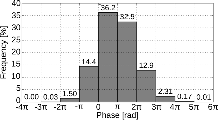
Fig. 2: Histogram of predicted phases. The target phases have a range of $\left[0,2\pi\right]$, but the predicted phases have a range of $\left[-4\pi,6\pi\right]$. All frames and frequency bins of the evaluation data in 　Section 4.1 are represented in this figure.

The generalized version of the von Mises distribution is the generalized cardioid distribution [17] given as

$$P^{(\rm GC)}\left(y_{t,f};\mu,\kappa,\psi\right) =$$

$$\frac{\left(\cosh\left(\kappa\psi\right)\right)^{1/\psi}\left(1+\tanh\left(\kappa\psi\right)\cos\left(y_{t,f}-\mu\right)\right)^{1/\psi}}{2\pi P_{1/\psi}\left(\cosh\left(\kappa\psi\right)\right)},$$ (8)

where $P_{1/\psi}$ is the associated Legendre function of the first kind of degree $1/\psi$ and order 0. The von Mises distribution is the special case ($\psi\rightarrow 0$) of this distribution. Also, this distribution is equivalent to the cardioid distribution and the wrapped Cauchy distribution for $\psi=1$ and $\psi=-1$, respectively. The negative log likelihood for $\mu$ for the cardioid and wrapped Cauchy distributions are equal to Eq. (2). Therefore, DNNs with these two distributions are trained in the same manner. One possible way to extend our work is to model phases using this generalized cardioid distribution. Other possible ways are to use an asymmetric distribution [18] and mixture model.

As described in 　Section 3.2.1, the phase loss is minimized when ${\hat{y}}_{t,f}=y_{t,f}\pm 2\pi N$ for arbitrary $N$. Therefore, von-Mises-distribution DNNs suffer from an exploding value of ${\hat{y}}_{t,f}$. To investigate this, Fig. 2 plots a histogram of the predicted phase spectrograms. We can see that the predicted phase spectrograms have a wider range than the target phase ($\left[0,2\pi\right]$), but the value does not explode.

4 Experimental evaluation

4.1 Experimental setup

Evaluations were performed using the JSUT corpus [19], a free Japanese speech corpus uttered by a female speaker. We used 5,000 utterances (approx. 6 hours) of the subset BASIC5000 for training and 300 utterances of the subset ONOMATOPEE300 for evaluation. Speech signals were downsampled at a rate of 16 kHz. The window length, shift length, and FFT length were set to 400 samples (25 ms), 80 samples (5 ms), and 512 samples, respectively. The Hamming window was used. Features fed to a DNN were the joint vectors of the log amplitude spectra at current and $\pm 2$ frames, and they were normalized to have zero-mean unit-variance. The DNN architectures were Feed-Forward networks that included $3\times 1024$-unit gated linear unit [20] hidden layers. The activation of the output layer was a linear function. We empirically explored DNN architectures within Feed-Forward networks and found that the gated linear unit is significantly better than a rectified linear unit (ReLU) [21] or LeakyReLU [22] hidden units. The DNN parameters were randomly initialized and the AdaGrad algorithm [23] with its learning rate set to 0.001 was used for the optimization algorithm.

We compared the conventional Griffin-Lim and three proposed phase reconstruction methods.

• only phase loss (Eq. (3))

• only group-delay loss (Eq. (6))

• multi-task learning (Eq. (7))

In the Griffin-Lim method, phase spectrograms were randomly initialized. The number of iterations was set to 100. The weight $\alpha$ for multi-task learning was set to $0.1$. In the proposed methods, phases in the low frequency band are first estimated by DNNs, and those in the remaining frequency bins are randomly generated. We used three settings of frequency bands of the predicted phase spectrograms: 0-2 (96 dim.), 0-4 (128 dim.), and 0-8 kHz (257 dim.). After predicting the phase spectrogram by DNNs, we further applied the Griffin-Lim method to refine the phase. The number of iterations of the phase refinement was 100.

4.2 Prediction accuracy

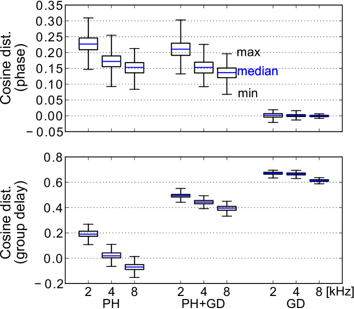
Fig. 3: Box plots of cosine distances between target and predicted phases (upper) and group delays (lower). The box indicates the first and third quartiles.

Table 1: Results of preference tests: conventional Griffin-Lim method vs. proposed methods. Bold indicates preferred method that has a $p$-value smaller than $0.05$

Method A	Scores	$p$-value	Method B
Griffin-Lim	0.497 vs. 0.503	0.871	PH (2 kHz)
Griffin-Lim	0.280 vs. 0.720	$<10^{-9}$	PH (4 kHz)
Griffin-Lim	0.277 vs. 0.723	$<10^{-9}$	PH (8 kHz)
Griffin-Lim	0.453 vs. 0.547	0.022	PH+GD (2 kHz)
Griffin-Lim	0.233 vs. 0.767	$<10^{-9}$	PH+GD (4 kHz)
Griffin-Lim	0.247 vs. 0.753	$<10^{-9}$	PH+GD (8 kHz)
Griffin-Lim	0.447 vs. 0.553	0.009	GD (2 kHz)
Griffin-Lim	0.463 vs. 0.537	0.073	GD (4 kHz)
Griffin-Lim	0.490 vs. 0.510	0.619	GD (8 kHz)

We evaluated prediction accuracies of phases and group delay. Fig. 3 shows cosine distances between target and predicted phases and group delays. The distances were averaged over all frames and frequency bins of the predicted phases (0-2, 0-4, or 0-8 kHz).

The prediction accuracy of “PH (2 kHz)” ranges from $0.15$ to $0.31$, and the distribution seems symmetric. Also, the accuracy becomes smaller as the frequency band widens (“PH (4, 8 kHz)”). This result is natural because phases at higher frequency bins are easily changed by the temporal position of frame analysis. On the other hand, when using only group-delay loss (“GD”), group delay can be predicted more accurately than phase for all settings of frequency bands. This result shows us that the Feed-Forward DNN can predict group delay better than phases themselves. Finally, combined phase loss and group-delay loss (“PH+GD”) predicts phase more accurately than “GD” and group delay more accurately than “PH” for all settings of frequency bands. Therefore, we can demonstrate the effectiveness of the proposed multi-task training.

4.3 Comparison of Griffin-Lim and proposed methods

To evaluate the effectiveness of the proposed methods, we compared the quality of synthetic speech of Griffin-Lim and proposed methods. Preference AB tests (listening tests) on speech quality were performed in our crowdsourcing evaluation system. 30 listeners participated in each test. Approximately $\$0.46$ were paid to each listener. Each listener preferred better-quality speech and answered for ten pairs of samples, i.e., 300 answers were obtained in each evaluation. Speech samples of pairs of methods were randomly presented to the listeners. These settings are also used not only here but also in the following sections.

Table 1 lists the results. The proposed methods outperform the conventional Griffin-Lim method in all settings of loss functions and frequency bands. In particular, “PH+GD” always has significantly better scores than the conventional Griffin-Lim method. These results demonstrate the effectiveness of the proposed methods.

4.4 Effect of phase refinements

Fig. 4: Box plots of cosine distances between predicted and refined phases (upper) and group delays (lower). The box indicates the first and third quartiles.

Table 2: Results of preference tests: proposed methods with different frequency bands. Bold indicates preferred method that has a $p$-value smaller than $0.05$

Method A	Scores	$p$-value	Method B
PH (2 kHz)	0.270 vs. 0.730	$<10^{-9}$	PH (4 kHz)
PH (4 kHz)	0.507 vs. 0.493	0.744	PH (8 kHz)
PH+GD (2 kHz)	0.223 vs. 0.777	$<10^{-9}$	PH+GD (4 kHz)
PH+GD (4 kHz)	0.493 vs. 0.507	0.744	PH+GD (8 kHz)
GD (2 kHz)	0.513 vs. 0.487	0.514	GD (4 kHz)
GD (4 kHz)	0.567 vs. 0.433	0.001	GD (8 kHz)

As explained in 　Section 4.1, after phases were predicted by DNNs, they were refined by the Griffin-Lim method. Here, we evaluated effects of the phase refinements. Fig. 4 shows cosine distances between predicted and refined phases and group delays. Tendencies were almost the same as those in Fig. 3. When phase loss is used in training (“PH” and “PH+GD”), phase information is comparably preserved. Similarly, when group-delay loss is used in training (“GD” and “PH+GD”), the group-delay information is comparably preserved. In the preliminary evaluation, we compared speech quality of refined and unrefined phases (i.e., phases predicted by DNNs were directly used for finally synthesized speech). The results demonstrated that unrefined phases had significantly worse speech quality than refined phases.

4.5 Effect of frequency bands

We compared effects of frequency bands of predicted phases within one loss function (“PH”, “PH+GD”, or “GD”). Table 2 shows the results of preference AB tests on speech quality. In “PH” and “PH+GD,” speech quality for 0-4 kHz frequency bands is significantly better than that for 0-2 kHz, and is comparable with that for 0-8 kHz. These results suggest that at least 0-4 kHz frequency bands needs to be predicted but the spectrograms in the higher frequency bands may be excited by random phases (this tendency is similar to the harmonics plus noise model [24]). A curious point is that “GD” has different tendencies: speech quality for 0-8 kHz frequency bands was significantly worse than that for 0-4 kHz. We will investigate the reason for this.

4.6 Effect of group-delay loss

We investigated the effectiveness of group-delay loss compared with phase loss. First, we evaluated convergence of phase refinements. Fig. 5 shows the log spectral convergence [25] of “PH (4 kHz)” and “PH+GD (4 kHz).” For comparison, results of randomized initialization of phases are also shown as “Random.” The proposed methods (“PH (4 kHz)” and “PH+GD (4 kHz)”) have a smaller value for the spectral convergence than “Random.” Also, “PH+GD (4 kHz)” has a smaller value than “PH (4 kHz)”, i.e., “PH+GD (4 kHz)” is the closest to the perfect reconstruction.

Fig. 5: Log spectral convergence by phase refinements. When the value is $-\infty$, perfect reconstruction through STFT and inverse STFT is achieved. This is the result of one of the evaluation datasets, but the same tendency was observed in all evaluation datasets.

In addition, we compared speech quality of “PH” and “PH+GD.” Table 3 lists the results of the comparison with frequency bands of 0-2, 0-4, and 0-8 kHz. “PH” is preferred more in 0-8 kHz with statistical significance, but “PH+GD” is preferred more in 0-2 and 0-4 kHz (without statistical significance). Therefore, we can demonstrate the effectiveness of group-delay loss in speech quality.

Table 3: Results of preference tests: effects of group-delay loss. Bold indicates preferred method that has a $p$-value smaller than $0.05$

Method A	Scores	$p$-value	Method B
PH (2 kHz)	0.487 vs. 0.513	0.514	PH+GD (2 kHz)
PH (4 kHz)	0.486 vs. 0.514	0.500	PH+GD (4 kHz)
PH (8 kHz)	0.545 vs. 0.455	0.031	PH+GD (8 kHz)

5 Conclusion

This paper presented DNN-based phase reconstruction from an amplitude spectrogram. Based on maximum likelihood estimation of the von Mises distribution, we introduced two loss functions for DNN training: phase loss and group-delay loss. We demonstrated 1) the trained DNNs can predict group delay more accurately than phases, and 2) our proposed phase reconstruction methods achieve better speech quality than the conventional Griffin-Lim phase reconstruction method. For future work, we will implement other probability distributions for periodic variables, propose other approaches for phase refinements, and integrate our method with text-to-speech synthesis that generates amplitude spectrograms [4].

Acknowledgments: Part of this work was supported by SECOM Science and Technology Foundation, and JSPS KAKENHI Grant Number 18K18100.

References

- [1] H. Zen, K. Tokuda, and A. Black, “Statistical parametric speech synthesis,” Speech Communication, vol. 51, no. 11, pp. 1039–1064, 2009.
- [2] S. Takaki, H. Kameoka, and J. Yamagishi, “Direct modeling of frequency spectra and waveform generation based on phase recovery for DNN-based speech synthesis,” in Proc. INTERSPEECH, Stockholm, Sweden, Aug. 2017.
- [3] Y. Wang, RJ Skerry-Ryan, D. Stanton, Y. Wu, Ron J. Weiss, N. Jaitly, Z. Yang, Y. Xiao, Z. Chen, S. Bengio, Q. Le, Y. Agiomyrgiannakis, R. Clark, and R. A. Saurous, “Tacotron: Towards end-to-end speech synthesis,” vol. abs/1609.03499, 2017.
- [4] Y. Saito, S. Takamichi, and H. Saruwatari, “Text-to-speech synthesis using stft spectra based on low-/multi-resolution generative adversarial networks,” in Proc. ICASSP, Calgary, Canada, Apr. 2018, pp. 5299–5303.
- [5] D. W. Griffin and J. S. Lim, “Signal estimation from modified short-time fourier transform,” IEEE Transactions on Acoustics, Speech and Signal Processing, vol. 32, no. 2, pp. 236–243, Apr. 1984.
- [6] I. Goodfellow, J. Pouget-Abadie, M. Mirza, B. Xu, D. WardeFarley, S. Ozair, A. Courville, and Y. Bengio, “Generative adversarial nets,” Proc. NIPS, pp. 2672––2680, 2014.
- [7] Y. Saito, S. Takamichi, and H. Saruwatari, “Statistical parametric speech synthesis incorporating generative adversarial networks,” IEEE/ACM Transactions on Audio, Speech, and Language Processing, vol. 26, no. 1, pp. 755–767, Jun. 2018.
- [8] Y. Li, K. Swersky, and R. Zemel, “Generative moment matching networks,” in Proc. ICML, Lille, France, Jul. 2015, pp. 1718–1727.
- [9] S. Takamichi, K. Tomoki, and H. Saruwatari, “Sampling-based speech parameter generation using moment-matching network,” in Proc. INTERSPEECH, Stockholm, Sweden, Aug. 2017, pp. 3961–3965.
- [10] H. Zen, A. Senior, and M. Schuster, “Statistical parametric speech synthesis using deep neural networks,” in Proc. ICASSP. Vancouver, Canada, May 2013.
- [11] Z. Wu and S. King, “Minimum trajectory error training for deep neural networks, combined with stacked bottleneck features,” in Proc. INTERSPEECH, Dresden, Germany, Sep. 2015, pp. 309–313.
- [12] K. Hashimoto, K. Oura, Y. Nankaku, and K. Tokuda, “The effect of neural networks in statistical parametric speech synthesis,” in Proc. ICASSP, Brisbane, Australia, Apr. 2015, pp. 4455–4459.
- [13] K. V. Mardia and P. E. Jupp, Directional Statistics, John Wiley & Sons Ltd., 1999.
- [14] I.T. Nabney, C.M. Bishop, and C. Legleye, “Modelling conditional probability distributions for periodic variables,” in 1995 Fourth International Conference on Artificial Neural Networks, Calgary, Canada, Jun. 1995, pp. 177–182.
- [15] F. Itakura and T. Umezaki, “Distance measure for speech recognition based on the smoothed group delay spectrum,” in Proc. ICASSP, Dallas, U.S.A., Apr. 1987, pp. 1257–1260.
- [16] R. Padmanabhan, S. H. K. Parthasarathi, and H. A. Murthy, “Robustness of phase based features for speaker recognition,” in Proc. INTERSPEECH, Brighton, U. K., Sep. 2009, pp. 2355–2358.
- [17] M. C. Jones and Arthur Pewsey, “A family of symmetric distributions on the circle,” Journal of the American Statistical Association, vol. 100, no. 472, pp. 1422–1428, Dec. 2005.
- [18] T. Abe and A. Pewsey, “Sine-skewed circular distributions,” Statistical Papers, vol. 52, no. 3, pp. 683–707, Aug. 2011.
- [19] R. Sonobe, S. Takamichi, and H. Saruwatari, “JSUT corpus: free large-scale japanese speech corpus for end-to-end speech synthesis,” vol. abs/1711.00354, 2017.
- [20] Y. N. Dauphin, A. Fan, M. Auli, and D. Grangier, “Language modeling with gated convolutional networks,” vol. abs/1612.08083, 2016.
- [21] X. Glorot, A. Bordes, and Y. Bengio, “Deep sparse rectifier neural networks,” in Proc. AISTATS, Lauderdale, U.S.A., Apr. 2011, pp. 315–323.
- [22] L. A. Maas, Y. A. Hannun, and Y. A. Ng, “Rectifier nonlinearities improve neural network acoustic models,” in Proc. ICML, 2013, vol. 30.
- [23] J. Duchi, E. Hazan, and Y. Singer, “Adaptive subgradient methods for online learning and stochastic optimization,” EURASIP Journal on Applied Signal Processing, vol. 12, pp. 2121––2159, 2011.
- [24] Y. Stylianou, “Applying the harmonics plus noise model in concatenative speech synthesis,” IEEE Transactions on Speech and Audio Processing, vol. 9, no. 1, pp. 21–29, Jun. 2001.
- [25] N. Sturmel and L. Daudet, “Signal reconstruction from STFT magnitude: A state of the art,” in Proc. of 14th International Conference on Digital Audio Effects DAFx-11, Paris, France, Sep. 2011, pp. 177–182.