Wide-field Infrared Survey Explorer (WISE) Catalog of Periodic Variable Stars

Abstract

We have compiled the first all-sky mid-infrared variable-star catalog based on Wide-field Infrared Survey Explorer (WISE) five-year survey data. Requiring more than 100 detections for a given object, 50,282 carefully and robustly selected periodic variables are discovered, of which 34,769 (69%) are new. Most are located in the Galactic plane and near the equatorial poles. A method to classify variables based on their mid-infrared light curves is established using known variable types in the General Catalog of Variable Stars. Careful classification of the new variables results in a tally of 21,427 new EW-type eclipsing binaries, 5654 EA-type eclipsing binaries, 1312 Cepheids, and 1231 RR Lyraes. By comparison with known variables available in the literature, we estimate that the misclassification rate is 5% and 10% for short- and long-period variables, respectively. A detailed comparison of the types, periods, and amplitudes with variables in the Catalina catalog shows that the independently obtained classifications parameters are in excellent agreement. This enlarged sample of variable stars will not only be helpful to study Galactic structure and extinction properties, they can also be used to constrain stellar evolution theory and as potential candidates for the James Webb Space Telescope.

1 Introduction

Periodic variable stars exhibit regular or semi-regular luminosity variations. They are usually discovered through time-domain surveys. The period is usually related to the object’s physical or geometric properties. The masses, luminosities, radii, and ages of variable stars can be partially evaluated on the basis of their periods. Therefore, variables are important objects not only to study Galactic structure, but also for constraining stellar evolution. Among the wide diversity of variable stars, classical Cepheids are the most important distance tracers used to establish the cosmological distance scale.

Before the 1990s, many thousands of periodic variable stars were found and studied, often in individual papers. After the 1990s, large-scale surveys became available and the number of periodic variable stars increased rapidly. The Massive Compact Halo Object survey (MACHO; Alcock et al., 1993) found some 20,000 variable stars in the Large Magellanic Cloud (LMC). Over the course of more than 20 years, the Optical Gravitational Lensing Experiment (OGLE), releases I–IV (Udalski et al., 1994, 2015), detected more than 400,000 variable stars in the Magellanic Clouds and the Galactic bulge. A Fourier method was developed to classify different types of variables (Soszynski et al., 2008a, b; Soszynski et al., 2009). This survey directly led to a better understanding of the distance to and structure of the LMC (Pietrzynski et al., 2013; Inno et al., 2016).

The All Sky Automated Survey (ASAS; Pojmanski et al., 1997) was the first survey to cover almost the entire sky, probing objects down to $V\sim 14$ mag. The resulting catalog contained of order 10,000 eclipsing binaries and 8000 periodic pulsating stars (Pojmanski et al., 2005). Similar surveys in the $R$ band were the Robotic Optical Transient Search Experiment (ROTSE; Akerlof et al., 2000) and, subsequently, the Northern Sky Variability Survey (NSVS; Wozniak et al., 2004); Hoffman et al. (2009) identified 4659 periodic variable objects in the NSVS. Recently, near-Earth object (NEO) surveys have provided new opportunities to find additional periodic variables. Sesar et al (2011) and Palaversa et al. (2013) found and classified 7000 variables in the course of the Lincoln Near-Earth Asteroid Research (LINEAR). Significant progress was made in the context of the Catalina Sky Survey’s Northern (Drake et al., 2014) and Southern (Drake et al., 2017) catalogs, which identified some 110,000 periodic variable stars with magnitudes down to $V\sim 20$ mag. This massively increased the sample of eclipsing binaries and RR Lyrae, which has resulted in a better understanding of both the solar neighborhood and the structure of the Galactic halo (Drake et al., 2013; Chen et al., 2018). Nevertheless, all of these surveys were conducted at optical wavelengths, which prevented detailed studies of the heavily reddened Galactic disk. The VISTA Variables in Vía Láctea (VVV) team conducted a near-infrared (NIR) ${K_{\rm s}}$-band multi-epoch survey of the Galactic bulge and southern disk. They found 404 RR Lyrae in the southern Galactic plane (Minniti et al., 2017).

The study of variables in the infrared has great potential given the current availability of the Spitzer Space Telescope and the Wide-field Infrared Survey Explorer (WISE), and also in view of the soon to be launched James Webb Space Telescope (JWST). Studies of variables in the infrared view can benefit our understanding of infrared extinction, since the universality (or otherwise) of the infrared extinction law is still being debated (e.g. Matsunaga et al., 2018). Studies using the red clump as a diagnostic tool imply a relatively universal extinction law in the NIR but a variable mid-infrared (MIR) extinction law (Wang & Jiang, 2014; Zasowski et al., 2009). Compared to using the red clump, samples of periodic variables can be isolated and identified much better. Cepheids and RR Lyrae, well-understood secondary distance tracers, can also be used to study the structure of and distances to the Galactic arms, bulge, bar, and center. Matsunaga et al. (2011) first detected three classical Cepheids in the Galactic Center’s nuclear stellar disk based on NIR photometry. Feast et al. (2014) traced the flaring of the outer disk based on five classical Cepheids using both optical and NIR photometry. The spiral arm are expected to be delineated by these variables. In addition, the number of stars accompanied by dust shells or disks will increase prominently if selections are based on infrared observations. This provides additional opportunities to better understand the physical properties of Miras, semi-regular variables, Be stars, and many other types of variables.

In this paper, we collect the five-year WISE data to detect periodic variables across the entire sky. More than 50,000 high-confidence variables are found, filling the gaps in the Galactic plane. An all-sky variable census is achieved down to a magnitude $W1\sim 14$ mag ($G\sim 16$ mag). Light-curve and photometric analyses are used to classify the variables. More than 34,000 new variables are found. The data are described in Section 2. The methods adopted to identify and classify variables are discussed in Sections 3 and 4, respectively. Our new variable catalog and a comparison of its properties with previously published parameters are included in Section 5. Section 6 presents the light curves of different variables and Section 7 concludes the paper.

2 WISE multi-epoch data

WISE is a 40 cm (diameter) space telescope with a $47^{\prime}\times 47^{\prime}$ field of view. It was designed to conduct an all-sky survey in four MIR bands, $W1$ (3.35 $\mu$m), $W2$ (4.60 $\mu$m), $W3$ (11.56 $\mu$m), and $W4$ (22.09 $\mu$m). WISE began to operate in survey mode in 2010 January; it covers the full sky once every half a year (Wright et al., 2010). The solid hydrogen cryostat was depleted in 2010 September, upon which a four-month NEOWISE Post-Cryogenic Mission (Mainzer et al., 2011) continued to accomplish the second all-sky coverage. The data resulting from these two epochs were packaged as the ALLWISE Data Release, characterized by an enhanced accuracy and sensitivity compared to the WISE All-Sky Data Release. Next, WISE entered into a hibernating state for two years and was reactivated in 2013 October. WISE operations are currently continuing with a mission called the ‘near-Earth object WISE reactivation (NEOWISE-R) mission’. At present, four years of NEOWISE-R data have been released.

Without cryogen, NEOWISE-R only performs photometry in two bands, $W1$ and $W2$. Therefore, by combining ALLWISE and NEOWISE-R, five whole years and photometric data covering at least 10 epochs are available for each object. During each epoch, some 10–20 images were taken of any one field with intervals of 0.066 or 0.132 days; the total exposure time for a given epoch ranged between 1.1 and 1.4 days. The majority of stars have more than 100 detections and variables with periods in the range of 0.14–10 days can be identified adequately. The zeropoint differences between ALLWISE and NEOWISE-R were discussed in detail by Mainzer et al. (2011); a systematic difference of $\sim$0.01 mag and a statistical scatter of 0.03–0.04 mag for $8<W1<14$ mag and $7<W2<13$ mag were found. The angular resolution of WISE, as a function of passband at increasing wavelengths is $6.1^{\prime\prime},6.4^{\prime\prime},6.5^{\prime\prime}$, and $12.0^{\prime\prime}$, which is much lower than that of the Two Micron All Sky Survey (2MASS; Cutri et al., 2003). To reduce blending, 2MASS photometry was used to assist. The combination of NIR and MIR photometry was also used to select variable stars exhibiting infrared excesses.

The ALLWISE and NEOWISE-R catalogs contain about 100 billion rows of data for 0.7 billion individual objects. This is simply too large a number to access the entire database and perform the analysis. Therefore, we only focused on objects that are high-probability variables, i.e., with AllWISE Source Catalog keyword ‘var_flg’ = 6, 7, 8, or 9. Although this selection could potentially omit a small number of variables, it is indeed helpful to avoid the detection of pseudo-light variations. The total number of candidates is 2.7 million. Data pertaining to multi-epoch photometry was collected by selecting angular distances of less than $1^{\prime\prime}$ for any given object. Detections with ‘null’ magnitude uncertainties were excluded, since their magnitudes were either not measurable or 95% confidence-interval upper limits. This selection criterion also excludes photometry with poor signal-to-noise ratios, $snr=$ ‘null,’ and poor reduced $\chi^{2}$ resulting from the profile fits, $rchi2=$ ‘null.’ $qi\_fact>0,saa\_sep>0,moon\_masked=0$, and $qual\_frame>0$ were adopted to exclude other types of contamination or biases: $qual\_fact$ is the frame quality score, which ranges from 0 to 10 (0 represents the lowest quality, i.e., sources that are spurious detections due to noise noise, or objects affected by transient events or scattered light), $qi\_fact$ is the image quality score (where $qi\_fact=0$ represents the lowest quality), and $saa\_sep$ is the distance to the boundary of the South Atlantic Anomaly, in degrees ($saa\_sep>0$ means that WISE is on the outside). Finally, $moon\_masked=0$ denotes that the frame is not located in the moon-masked area.

3 Identification of periodic variables

To identify periodic variables, the Lomb–Scargle periodogram (Lomb, 1976; Scargle, 1982) method was adopted. The input frequency ranged from 0.01 to 7 day^-1 with a step length of 0.0001 day^-1, so it covered periods between 0.143 and 10 days, with an ideal accuracy of better than 0.01%. Periods were derived from the frequency associated with the maximum power spectral density (PSD). The standard deviation of the frequencies, $\sigma_{50\%}$, and $\sigma_{95\%}$ were estimated based on PSDs greater than 50% and 95% of the maximum PSD, respectively. The preliminary period uncertainty, $\sigma_{1}(P)$, was estimated based on the latter. $\sigma_{50\%}<0.21$ and $\sigma_{1}(P)/P<0.20$ were used to select variable candidates; $\sigma_{50\%}=0.21$ is the boundary where the peak becomes flat. This selection resulted in a rate of false noise of less than 10%. Then, we adopted a fourth-order Fourier analysis $\displaystyle{f=a_{0}+\sum_{i=1}^{4}a_{i}\cos(2\pi it/P+\phi_{i})}$ to fit each light curve, and adjusted $R$-square ($R^{2}>0.7$) and root-mean-squared error (RMSE $<$ 0.05) were combined to select candidates. The phase idleness rate was estimated using a bin size of 0.01, and objects with idleness rates greater than 50% were excluded. In addition, objects with poorly fitting light curves were excluded through higher-order amplitude selection, $a_{3}>0.08$ mag or $a_{4}>0.08$ mag. After application of these selection criteria, 68,034 candidates remained.

Based on a visual check of the light curves of some candidate variables, it became clear that major problems were caused by the imhomogeneous distribution of the data points. This would lead to the derivation of incorrect periods. The data were divided into five bins, by phase, without enforcing a fixed starting point, and the number probability, mean deviation, and scatter around the best-fitting Fourier line in each bin were estimated. Note that the mean deviation and scatter were given in units of total amplitude. These three parameters were used to exclude objects located outside the $3\sigma$ boundaries for any given selection choice and outside $1\sigma$ for all three selection criteria. The objects thus excluded were flagged as suspected variables, since their period could likely be improved with larger numbers of detections.

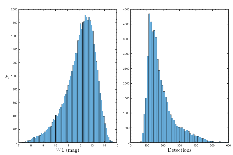
Figure 1: Number distribution of (left) $W1$ magnitudes and (right) $W1$ detections for our 50,296 variables.

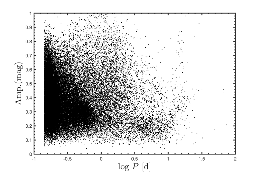
Figure 2: Amplitude versus period diagram for the 50,296 variables.

The final selection step aimed at excluding objects with unstable periods, especially among long-period objects. The best periods were determined using the four- and five-year data separately. Objects with period differences in excess of 10% were also excluded as suspected variables. The remaining objects comprised our sample of high-confidence variables. The period difference was treated as a second period uncertainty, $\sigma_{2}(P)$, and the final period uncertainty was the larger of $\sigma_{1}(P)$ and $\sigma_{2}(P)$. The total number of variables thus obtained was 50,296. The $W1$ magnitude distribution of these variables is shown in the left-hand panel of Figure 1. Most are in the magnitude range $8<W1<14$ mag, where the zeropoint differences between ALLWISE and NEOWISE-R are negligible. The right-hand panel of Figure 1 shows the $W1$-band detection numbers, with a upper limit of 600 (489 variables have more than 600 detections). We can infer that only 2853 variables have fewer than 100 detections, which means that our final sample of 50,296 variables is well-covered in the $W1$ band. Figure 2 is the amplitude versus period diagram, which is used to detect false positives. False signals due to sampling patterns would produce a random distribution in amplitude for a given period (Drake et al., 2014). Based on Figure 2, we assert that no such false signals are detected among our 50,296 variables.

4 Classification of periodic variables

To classify the types of periodic variables, their colors, periods, and shapes of the light curves were used. We tested our classifications using variables with known classifications from the General Catalog of Variable Stars (GCVS). In the magnitude detection range of WISE, 80%, 60%, 49%, 46%, 43%, and 42% of EW-type eclipsing binaries (EWs), classical Cepheids (Cep-Is), Type-ab RR Lyrae (RRab), EA-type eclipsing binaries (EAs), Type-c RR Lyrae (RRc), and Type II Cepheids (Cep-IIs) were confirmed. We did not detect Mira variables because of their long periods. Therefore, we used GCVS Miras to analyze the infrared excesses of our sample Miras. To guide our classification, Figure 3 shows the distributions of variables using different parameters.

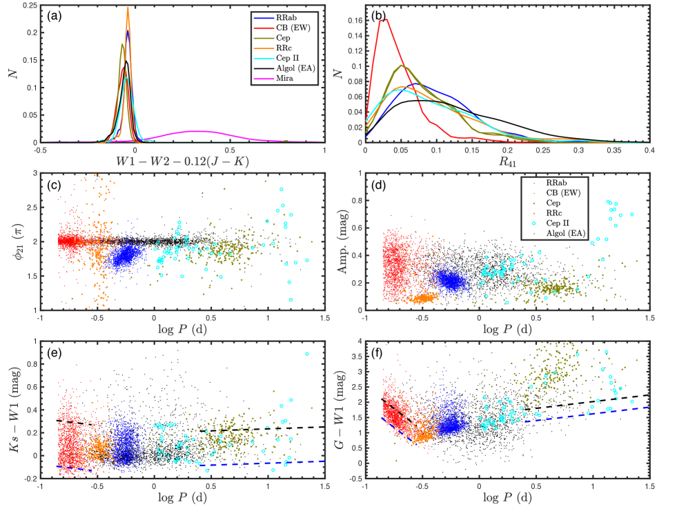
Figure 3: The different colors and symbols denote different types of variables. Blue: RRab; red: EWs; light green: Cep-Is; orange: RRc; cyan: Cep-IIs; black: EAs; magenta: Miras. The six panels show the parameters used to classify our variables: infrared excess index (a), period (b, d, e, f), phase difference (b, c), amplitude ratio (c), full amplitude (d), ${K_{\rm s}}-W1$ color (e), and $G-W1$ color (f). The black and blue dashed lines in panels (e) and (f) are the intrinsic colors of contact binaries and classical Cepheids, respectively (Gaia Collaboration, 2017; Chen et al., 2018; Wang et al., 2018).

Infrared excess. Since the variable stars were selected in the infrared, a number of objects are expected to have intrinsic infrared excesses owing to the presence of circumstellar dust disks or shells. To exclude these objects from normal stars, Flaherty et al. (2007) adopted selection criteria $[3.6]-[4.5]<0.6$ mag and $[5.8]-[8.0]<0.2$ mag based on Spitzer photometry. The effective wavelengths of the WISE $W1$ and $W2$ bands are close to those of the Spitzer $[3.6]$ and $[4.5]$ filters. Because of the low accuracy of our $W3$ and $W4$ photometry, we adopted as selection criterion $W1-W2<0.12\times(J-{K_{\rm s}})$. This is somewhat stricter than Flaherty et al. (2007)’s $[3.6]-[4.5]<0.6$ mag, since most of the variables are characterized by $J-{K_{\rm s}}<5.0$ mag. Figure 3a shows the Gaussian kernel smooth density distributions of several types of variables. EAs, EWs, RRab, RRc, and Cep-Is all satisfy the criterion, while the evolved Miras entirely exceed it. Variables with infrared excess include not only Miras, but also Be stars, young stellar objects, and a small fraction of Cep-II.

Periods. Periods of variables are in part related to their luminosities and masses, so different types of variables have characteristic periods. In Figure 3d, e, and f, different colors and symbols denote the period distribution of these variables (for eclipsing binaries we provide half periods). From short to long periods, we encounter EWs, RRc, RRab, EAs, Cep-Is and Cep-IIs. Although EW-type eclipsing binaries are found with periods ranging from 0.19 days to a few dozen days, the vast majority have periods of less than 1 day. EA-type eclipsing binaries also span a wide period range. However, the majority have periods longer than 1 day. The period ranges of RRc and RRab are relatively concentrated: $0.16<P<0.50$ days and $0.32<P<1.00$ days, respectively (Clementini et al., 2018). Cep-IIs were divided into three subtypes: BL Herculis (BL Her), W Virginis (W Vir), and RV Tauri (RV Tau), with the corresponding period ranges $1.0\leq P<4.0$ days, $4.0\leq P<20.0$ days, and $P\geq 20.0$ days (Soszynski et al., 2008b). In this paper, we could only detect BL Her and W Vir variables. The periods of Cep-Is are usually longer than 2.24 days (Gaia Collaboration, 2017).

Colors. Since the distances to our variables are usually unknown, we adopted their intrinsic colors instead of their absolute magnitudes. EW-type eclipsing binaries are redder than main-sequence stars, and they become bluer for increasing orbital periods. RRab and RRc are bluer still and concentrated in a narrow color range (see also Drake et al., 2014). They become slightly redder for increasing periods, which is caused by changes in the bolometric correction. Cep-Is also become redder with increasing of period. Since Galactic Cep-Is are usually located in the heavily reddened mid-plane, they are often associated with significant extinction and reddening. Figure 3e and f shows the distributions of our variables in ${K_{\rm s}}-W1$ and $G-W1$ color vs. $\log P$ space. The intrinsic colors of contact binaries and Cepheids (Gaia Collaboration, 2017; Chen et al., 2018; Wang et al., 2018) are shown as the black and blue dashed lines, respectively, for reference. Note that Cep-IIs exhibit a wide spread in ${K_{\rm s}}-W1$ color, which is the result of their intrinsic infrared excesses rather than foreground reddening. For variables affected by low reddening, EWs are redder than $G-W1=1.0$ mag, RRcs are bluer than $G-W1=1.0$ mag, while RRab are found in the range of $1.0<G-W1<1.5$ mag. However, for variables affected by significant reddening, no color selection criteria are available, since ${K_{\rm s}}-W1$ is both reddening and temperature insensitive.

Light curves. The shape of the light curve is of key importance to distinguish among variables. In Figure 3c, eclipsing binaries have more symmetric light curves, which is reflected in the phase difference $\phi_{21}=\phi_{2}-2\phi_{1}$. This may deviate from $0$ or $2\pi$ (we adopt $2\pi$ uniformly) because of low photometric accuracy, low amplitude, or complexity in the light curve. In the WISE $W1$ band, 85% of EWs and 93% of EAs in the GCVS have phase differences in the range $|\phi_{21}-2\pi|<0.1\pi$. On the other hand, pulsating stars exhibit asymmetric light curves, which become more symmetric from optical to infrared wavelengths. Nevertheless, in the $W1$ band the asymmetry is still recognizable. The phase differences of RRab increase with period in the range of $[1.5-2.0]\pi$. RRc have a random distribution of $\phi_{21}$ because of their low amplitudes. Cep-Is have a phase difference in the range $\phi_{21}=[1.5-2.1]\pi$ for $2<P<10$ days and a random distribution around $P=10$ days. The global trend is similar to that in the $I$-band Fourier analysis based on the OGLE survey (Soszynski et al., 2008a). Our limited sample of Cep-IIs are more scattered than the classical Cepheids. The amplitude ratio $R_{41}=a_{4}/a_{1}$ could be used to distinguish EAs from other types of variables, since Cep-Is and EWs exhibit a cut-off at $R_{41}=0.25$ and $0.20$, respectively (see Figure 3b). The amplitude is the other characteristic parameter. Figure 3d shows the distribution of the best-fitting amplitudes. Note that the amplitudes were only used to classify the variables; the optimal amplitudes were redetermined after the classification step (see Section 5.4). Eclipsing binaries show a random distribution between 0.05 mag and 0.75 mag while pulsating stars are characterized by a more concentrated distribution. RRc have the lowest amplitudes (mostly less than 0.15 mag); the amplitude distribution of RRab and RRc is comparable to that of Gavrilchenko et al (2014). The amplitude of Cep-Is is usually smaller than 0.3 mag, while Cep-IIs show a wide distribution.

4.1 Variable types

Table 1: Criteria adopted to classify different variables

Type	Selection criteria
infrared excess variable	$W12JK>0$, $P>2.24$ d
RR	$0.316<P<1.0$ d, $\phi_{21}<1.9\pi$
Cep-I	$W12JK<0$, $P>2.24$ d, $\rm{Amp.}<0.5$ mag, $1.6\pi<\phi_{21}<2.1\pi$
Cep-I/Cep-II	$W12JK<0$, $P>2.24$ d, $\rm{Amp.}>0.5$ mag
	$W12JK<0$, $P>2.24$ d, $\rm{Amp.}<0.5$ mag, $|\phi_{21}-1.85\pi|>0.25\pi$
Cep-II/ACep/Cep-I	$1.0<P<2.24$ d, $\phi_{21}<1.9\pi$
Cep-I/EA	$P>2.24$ d, $W12JK<0$, $|\phi_{21}-2.0\pi|<0.12\pi$, $0.15<R_{31}<0.22$
Eclipsing binary	$0.16<P<0.316$ d, $\rm{Amp.}\geq 0.15$ mag
	$P<0.16$ d
	$0.316<P<1.0$ d, $\phi_{21}>2.1\pi$
	$P<2.24$ d, $|\phi_{21}-2.0\pi|<0.1\pi$
	$P>2.24$ d, $W12JK<0$, $|\phi_{21}-2.0\pi|<0.12\pi$, ($R_{21}>0.4$ or $R_{41}>0.15$)
Misc	$0.16<P<0.316$ d, $\rm{Amp.}<0.15$ mag
	$1.0<P<2.24$ d, $\phi_{21}>2.1\pi$
EW	$a_{4}<a_{2}(a_{2}+0.125)$
EA	$a_{4}>a_{2}(a_{2}+0.375)$
	$a_{2}(a_{2}+0.125)<a_{4}<a_{2}(a_{2}+0.375)$, $P>1.0$ d
EW/EA	$a_{2}(a_{2}+0.125)<a_{4}<a_{2}(a_{2}+0.375)$, $P<0.5$ d
EA/RR/EW	$a_{2}(a_{2}+0.125)<a_{4}<a_{2}(a_{2}+0.375)$, $0.5<P<1.0$ d

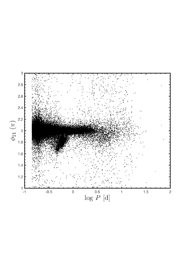
Figure 4: $\phi_{21}-\log P$ diagram defined by our 50,296 variables. The distribution is similar to Figure 3c. Eclipsing binaries are most obvious around $\phi_{21}=2\pi$. RRab and Cep-Is are found in two overdense regions, $-0.5<\log P<0.0$ and $\log P>0.5$, respectively (see also Figure 3c.

Employing the combination of these properties, EW- and EA-type eclipsing binaries, RR Lyrae, Cep-Is, Cep-IIs, and variables exhibiting an infrared excess could be classified (see Figure 4). Note that we did not use any color information, since many of our sample objects were reddened, so that intrinsic colors could not be determined. Table 1 lists the criteria adopted to classify the different types of variables. Infrared-excess variables were selected only for periods longer than 2.24 days, using $W12JK=W1-W2-0.12(J-{K_{\rm s}})>0$. Most were Miras and semi-regular variables (SRs), although small fractions of Cep-IIs, Be stars, and young stellar objects contaminated the selection. We were unable to detect any Miras or SRs with accurate periods, since the periods of these types of objects far exceed 10 days. Therefore, all such candidates were added to the suspected variables catalog.

Given the more symmetric MIR light curves, the boundary between RR Lyrae and eclipsing binaries was less obvious. Therefore, we only selected RR Lyrae exhibiting obvious asymmetries, $\phi_{21}<1.9\pi$, in the period range attributed to RR Lyrae; the remaining objects were classified as ‘EA/RR/EW.’ Compared with RRab, RRc have shorter periods and smaller amplitudes. They could not be easily classified. These latter objects are found mixed in with the EW, RR, and miscellaneous variables (‘Misc’). Cep-Is and Cep-IIs could be distinguished approximately by their amplitude and phase differences. EA-type objects were excluded from the Cep-I/II bin based on their larger amplitude ratio. The light curves of Cepheids were checked by eye to exclude long-period eclipsing binaries, because eclipsing binaries spend less time in the actual eclipse. Some 5–10% of the Cepheid subsample are likely eclipsing binaries. Anomalous Cepheids (ACeps) are mixed with Cep-Is and Cep-IIs in the period range $1.0<P<2.24$ days. The remaining variables were eclipsing binary candidates. Note that the parameter $P$ used in this case is the half-period of the eclipsing binaries. To distinguish between EW- and EA-type eclipsing binaries, we reran our Fourier analysis using the full periods. The curves $a_{4}=a_{2}(a_{2}+0.125)$ and $a_{4}=(a_{2}+0.375)$ were adopted to refine the EA and EW selection (see also Chen et al., 2018); $a_{2}$ and $a_{4}$ are the amplitudes of the second- and fourth-order Fourier series. Objects located near the boundary were classified as ‘EW/EA.’ A few hundred candidates showing asymmetric light curves across their full periods were reclassified as RR Lyrae. EB-type ($\beta$ Lyrae) eclipsing binaries could not be classified and are mixed with the EA and EW types (see also Drake et al., 2017). Variables such as RS CVn, $\delta$ Scuti objects, and rotating stars could not be classified since their MIR light curves did not provide sufficient characteristic features. These latter variables are either mixed with the other types or classified as Misc.

Table 2: WISE variables catalog .

ID	R.A.	Decl.	$<W1>$	Period	err${}_{P}/P$	Num	Amp.F10	Amp.10	Type	$R_{21}$	$\phi_{21}$	…
	∘	∘	mag	days			mag	mag			$\pi$	…
WISEJ094812.4$+$093448	147.05182	9.58021	11.667	0.6664177	0.00001	115	0.278	0.257	EA	0.504	2.041	…
WISEJ130034.1$-$211735	195.14238	$-$21.29326	11.306	0.6489507	0.00179	95	0.320	0.300	EW/EA	0.319	2.035	…
WISEJ125656.5$+$752821	194.23544	75.47264	8.298	1.6809747	0.00464	309	0.263	0.265	EW	0.103	2.139	…
WISEJ162004.0$+$451300	245.01694	45.21670	8.249	0.9836457	0.00269	269	0.163	0.169	EW	0.066	2.223	…
WISEJ164755.1$+$351756	251.97993	35.29889	12.118	0.6838987	0.00190	225	0.244	0.259	EW	0.186	2.076	…
WISEJ141332.8$+$031837	213.38667	3.31038	9.253	0.9079302	0.00002	114	0.175	0.147	EW	0.099	2.170	…
WISEJ113905.7$+$663017	174.77396	66.50495	11.343	1.6719398	0.00001	275	0.121	0.746	EW	0.029	2.703	…
WISEJ095035.2$+$354215	147.64679	35.70417	9.547	0.8519414	0.00165	116	0.196	0.182	EW	0.056	2.457	…
WISEJ151428.7$+$142730	228.61967	14.45854	10.535	1.0650266	0.00293	145	0.245	0.229	EW	0.171	2.049	…
WISEJ142230.6$+$012758	215.62791	1.46638	10.775	0.8127400	0.00001	129	0.204	0.210	EW	0.069	2.228	…
WISEJ145449.0$+$120526	223.70424	12.09083	12.677	0.7269519	0.00003	140	0.306	0.304	EW	0.230	2.103	…
WISEJ161622.5$+$243045	244.09389	24.51251	11.799	0.7506710	0.00001	162	0.254	0.218	EA	0.559	2.098	…
WISEJ102856.8$-$021733	157.23707	$-$2.29270	11.471	1.1148194	0.00004	133	0.296	0.268	EA/RR/EW	0.354	2.038	…
WISEJ102512.0$+$645138	156.30015	64.86075	10.079	0.7137239	0.00197	209	0.163	0.170	EW	0.086	2.288	…
WISEJ131817.1$-$123826	199.57147	$-$12.64065	12.707	0.8287763	0.00230	113	0.234	0.226	EW/EA	0.365	2.025	…
WISEJ125214.2$+$385630	193.05918	38.94193	10.723	0.6424413	0.00177	147	0.289	0.268	EW	0.213	2.034	…
WISEJ120251.4$+$334617	180.71442	33.77155	12.424	1.2186550	0.00335	156	0.341	0.306	EA/RR/EW	0.391	2.072	…
WISEJ101258.6$-$125418	153.24445	$-$12.90523	12.288	0.8111031	0.00157	110	0.249	0.247	EW	0.078	2.106	…
WISEJ141240.9$-$280107	213.17047	$-$28.01873	12.766	0.8297233	0.00228	126	0.237	0.251	EW	0.131	2.058	…
WISEJ095402.2$-$111655	148.50936	$-$11.28209	11.665	0.8831864	0.00245	98	0.204	0.206	EW	0.049	2.019	…
WISEJ170410.6$+$274628	256.04421	27.77450	13.833	0.7093259	0.00195	224	0.523	0.501	EW	0.248	2.024	…
WISEJ171731.0$+$524901	259.37949	52.81721	8.184	0.9313811	0.00180	418	0.210	0.223	EW	0.052	2.253	…
WISEJ122859.8$+$835851	187.24920	83.98096	13.078	0.7773740	0.00214	298	0.227	0.265	EW	0.118	2.048	…
WISEJ172508.1$+$371155	261.28400	37.19883	10.688	0.4412721	0.00242	227	0.222	0.243	RR	0.019	1.890	…
WISEJ123710.2$-$253930	189.29260	$-$25.65853	13.159	0.6405664	0.00247	99	0.319	0.325	RR	0.304	1.897	…
WISEJ092049.3$+$005246	140.20578	0.87956	8.014	1.2632250	0.00004	116	0.184	0.180	EW	0.051	2.016	…
WISEJ142750.2$-$203408	216.95948	$-$20.56915	12.344	0.7971740	0.00439	101	0.148	0.240	RR	0.090	1.933	…
WISEJ104541.0$-$203634	161.42120	$-$20.60958	8.648	0.6751995	0.00003	102	0.170	0.168	EA	0.560	2.060	…
WISEJ154116.9$+$744410	235.32058	74.73617	12.219	0.7267838	0.00003	612	0.158	0.218	EW	0.079	2.080	…
WISEJ171456.7$+$585128	258.73663	58.85789	11.724	0.8399786	0.00231	368	0.172	0.222	EW	0.057	2.926	…
WISEJ163216.0$+$750624	248.06705	75.10689	11.899	0.7972567	0.00155	335	0.141	0.160	EW	0.051	2.342	…
WISEJ151814.3$+$831733	229.55985	83.29276	11.418	1.7499784	0.00478	331	0.157	0.174	EW	0.156	2.167	…
WISEJ092206.6$-$103321	140.52763	$-$10.55590	13.094	0.6951391	0.00001	108	0.320	0.321	EW/EA	0.277	2.068	…
WISEJ072555.4$+$582631	111.48094	58.44205	12.777	0.6412162	0.00101	146	0.290	0.286	EW	0.092	2.146	…
WISEJ180409.2$+$445727	271.03869	44.95756	12.182	0.6664398	0.00129	342	0.127	0.161	EW	0.091	2.235	…
WISEJ052330.6$+$875817	80.87787	87.97140	12.968	0.8472612	0.00002	324	0.264	0.279	EW	0.076	2.172	…
WISEJ081021.7$+$324011	122.59043	32.66983	12.571	0.7071032	0.00001	106	0.349	0.336	EW/EA	0.273	2.071	…
WISEJ170425.6$+$061932	256.10676	6.32564	11.614	0.7263457	0.00199	134	0.233	0.225	EW	0.077	2.026	…
WISEJ163508.1$-$003634	248.78400	$-$0.60956	11.627	0.6934337	0.00134	127	0.368	0.406	EW	0.146	2.043	…
WISEJ180209.3$+$441950	270.53889	44.33074	12.520	1.4118240	0.00273	359	0.222	0.256	EW	0.062	2.122	…
WISEJ083550.2$+$071655	128.95934	7.28196	10.887	0.9797850	0.00002	110	0.271	0.273	EW	0.193	1.908	…
WISEJ081851.3$+$174326	124.71409	17.72396	11.021	0.7834653	0.00001	105	0.282	0.276	EW	0.146	2.125	…
WISEJ073939.5$+$611635	114.91497	61.27659	10.746	0.8453609	0.00188	158	0.304	0.296	EW	0.115	2.095	…
WISEJ174404.2$+$383837	266.01772	38.64386	11.511	1.0740403	0.00208	259	0.271	0.266	EW	0.117	2.059	…
WISEJ173801.7$+$183017	264.50747	18.50482	11.175	0.9878244	0.00191	178	0.213	0.223	EW	0.050	2.214	…
WISEJ174223.8$+$221438	265.59954	22.24398	9.984	1.0230755	0.00282	173	0.357	0.329	EW	0.200	2.039	…
WISEJ173400.2$+$161358	263.50118	16.23280	9.794	0.9762255	0.00188	157	0.224	0.221	EW	0.026	1.944	…
WISEJ075426.3$+$394659	118.60987	39.78321	11.627	1.1033470	0.00214	110	0.405	0.386	EA/RR/EW	0.435	2.054	…
WISEJ181228.7$+$544653	273.11978	54.78151	8.786	1.9013039	0.00518	436	0.090	0.107	EA/RR/EW	0.330	2.204	…
WISEJ173313.4$+$065117	263.30602	6.85493	11.627	0.9092463	0.00248	152	0.159	0.162	EW	0.089	2.425	…
…	…	…	…	…	…	…	…	…	…	…	…	…
…	…	…	…	…	…	…	…	…	…	…	…	…
…	…	…	…	…	…	…	…	…	…	…	…	…

5 The Catalog

The WISE catalog of variables, containing 50,282 periodic variables, is provided in Table 2. Fourteen known RRd-type variables have been excluded (see Section 5.2 and Table 4). Its column designations represent the following. ‘ID’ refers to the instrument and position, ‘SourceID’ is the number associated with the single exposure photometry catalog and ‘num’ is the number of detections. ‘$<W1>$, $<W2>$, Period, err${}_{P}/P$, and Amp._F10’ are the mean magnitudes in two bands, period, period uncertainty, and amplitude, respectively, determined by means of Fourier fitting. The other parameters resulting from the Fourier fits, $R_{21}=a_{2}/a_{1}$, $\phi_{21}=\phi_{2}-2\phi_{1}$, $a_{4}$, and $a_{2}$ are also listed. Amp.₁₀ is the direct amplitude in the 10–90% range of the magnitude distribution (see for details, Section 5.4) and ‘Type’ refers to the variable type. The NIR $J,H,{K_{\rm s}}$ magnitudes and the number of corresponding objects in 2MASS are found under the column headings ‘J,’ ‘H,’ ‘${K_{\rm s}}$,’ and ‘$\rm n_{2MASS}$,’ respectively. The single exposure photometry data and suspected variables catalog are available online, including their ‘SourceID,’ ‘R.A. (J2000),’ ‘Decl. (J2000),’ ‘MJD’ (modified Julian date), ‘W1mag’, ‘W2mag’, ‘e_W1mag’ and ‘e_W2mag’.

5.1 New variables

To validate our catalog, a comparison with known variables is required. The SIMBAD website provides a collection of almost all variables previously found in the Catalina, OGLE, and ASAS surveys, among others. We cross matched our 50,296 variables with SIMBAD positions using a $5^{\prime\prime}$ angular radius and selected those objects identified as variables. The majority of the known variables were found within angular radii of $1-2^{\prime\prime}$. The variables contained in the Catalina, OGLE, and ASAS catalogs were supplemented. We found that 15,527 objects had been found previously; the remaining 34,769 are new variables. Table 3 lists the statistics of the newly found variables. EW- and EA-type eclipsing binaries encompass the majority of the new variables; 1231 new RR Lyrae and 1312 new Cepheids were also found. Contamination levels were estimated based on comparisons of our classified types to the known types. For short-period variables such as EW and RR, the contamination fraction was around 5%, increasing to 10% for long-period variables. In total, 93% of our new classifications matched those previously obtained.

Table 3: Classification statistics of our 34,769 newly found periodic variables.

Type	Count	Fraction	Purity	Contamination
EW	21427	61.63%	95%	RR 2%, Ro 1%, EA 1%
EA	5654	16.26%	85%	EW 14%
RR	1231	3.54%	93%	EW 5% EA 1%
EA/RR/EW	1323	3.81%	71/16/12%
EW/EA	3036	8.73%	65/34%	RR 1%
Cep-I	583	1.68%	89%	Cep-II 3%, EA 3%, EW 2%, LPV 2%, Ro 1%
Cep-I/Cep-II	492	1.42%	57/25%	LPV 8%, EA 3%, EW 3%, Ro 3%
Cep-II/ACep/Cep-I	173	0.50%	40/29/21%	EA 3%, EW 3%, Ro 2%
Cep-I/EA	64	0.18%	74/22%	Cep-II 4%
Misc	786	2.26%
total	34769	100%

Figure 5 shows the distribution of the new variables in Galactic coordinates; 90% are located within $\pm 20^{\circ}$ of the plane, an area obscured in optical surveys. Most of the other new objects are located close to the equatorial poles, regions that were poorly sampled by the Catalina survey. A hole is present at the position of the LMC, where numerous variables were detected by the OGLE survey. The direction to the Galactic Center is also less populated, since the WISE detection efficiency decreases in crowded environments. Figure 6 shows the NIR color–magnitude diagram of these variables; colors denote the number of objects in bins of $0.035\times 0.055$ mag. Approximately 1000 objects have color excesses $E(J-K)>1.0$ mag, which implies that they are affected by $A_{K_{\rm s}}>0.5$ mag of extinction if we adopt the $A_{J}/A_{{K_{\rm s}}}=3.13$ NIR extinction law of Chen et al. (2018).

Figure 5: Distribution of our newly found variables in Galactic coordinates.

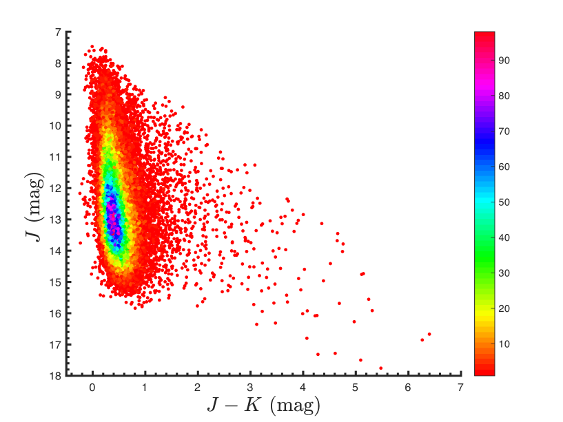
Figure 6: Scatter-density distribution in the NIR color–magnitude diagram. The color bar represents the number of objects per bin.

5.2 Comparison with the Catalina catalog

Compared with SIMBAD, the type classification in the Catalina catalog is more homogeneous and uniform. Therefore, we also performed one-to-one matches with the 110,000 variables in the Catalina catalog, again using a $5^{\prime\prime}$ angular radius for completeness, of which more than 10,000 objects matched. Table 4 reflects the detailed type comparison. The fraction of misclassifications is similar to that listed in Table 3. For EW-type variables, common contamination sources are RRc and rotating stars, since both types exhibit symmetric light curves. Multiple-period RRd-type variables comprise other types of contaminants. We have excluded them from our final sample, since their main periods were not properly determined in our analysis. For EA-type variables, EWs are the main contaminants. The same conclusion was drawn based on matching the Catalina and LINEAR catalogs (see Drake et al., 2014, Table 6). In optical bands, the boundary between RR Lyrae and eclipsing binaries is obvious and the fraction of misclassifications is less than 0.1%. However, in the MIR, approximately 6% of RR Lyrae are classified as eclipsing binaries. Some RR Lyrae show strong phase and amplitude modulations; they are known as RR Lyrae exhibiting the Blazkho effect. The effect is also visible but not obvious in the MIR, so we do not identify these objects separately. ‘EW/EA’ and ‘EA/RR/EW’ types indeed include high fractions of different types of variables, and no further classification refinements are possible. Most Cepheids in the Catalina catalog are Cep-IIs and ACeps, since the survey avoids the Galactic plane. The rate of contamination is a little higher than in the plane because of the smaller population of Cepheids here.

Table 4: WISE Variables matched with the Catalina catalog

Type	EW	EA	RRab	RRc	RRd	Blazkho	Cep-II	ACep	Rot.	$\delta$ Scuti	RS CVn
EW	7437	28	29	84	12	1	2	0	125	5	10
EA	106	640	0	0	0	0	5	1	3	0	1
RR	57	2	1114	10	0	33	1	5	6	0	1
EW/EA	611	218	0	2	1	0	0	0	1	1	0
EA/RR/EW	38	117	63	0	0	1	0	0	1	0	0
Cep	3	0	1	0	1	0	16	14	2	0	2

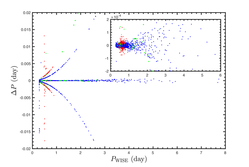
Figure 7: Period comparison with the Catalina catalog and $\Delta P=P_{\rm{Catalina}}-P_{\rm{WISE}}$. The blue, red, and green dots are eclipsing binaries, RRab, and other variables, respectively. Note that 92% of the variables are located on the central zero line. The top right-hand panel is a zoomed-in view of the variables characterized by $-0.0002<\Delta P<0.0002$.

We also compared our independently determined periods to those provided in the Catalina catalog. 98% of the variables have period differences $|\Delta P|<0.02$ days: see Figure 7. The other 2% of variables showing large differences are mainly eclipsing binaries. Their period difference is likely driven by the fact that the harmonic frequency or an adjusted frequency are adopted in the Catalina catalog. 92% of the variables have period differences of less than 0.001 day, and 76% have period differences of less than 0.0002 day. This implies that our MIR periods are as good as the optical periods.

Table 5: Completeness of WISE variables comparing to Catalina variables

Vmag (mag)	Completeness	Completeness (corrected)
$<11$	62.4%	91.4%
$<12$	57.5%	80.4%
$<13$	58.4%	82.0%
$<14$	50.3%	81.5%
$<15$	38.2%	78.6%
$<16$	25.9%	74.2%

5.3 Completeness

We also compared the sample of known Catalina variables with our rediscovered variables sample to evaluate the completeness of our catalog. Variables with amplitudes larger than 0.1 mag and periods in the range $0.28<P<15$ days are considered, since beyond these constraints few variables are detected in our catalog. The completeness for each magnitude range is listed in the second column of Table 5; its level decreases as the variables become fainter. In addition, variables with $V>16$ mag are more incomplete owing to the detection limit. The $\sim$50% completeness levels mean that our variables are highly affected by our selection procedure, which could be improved based on enhanced photometric data or in-depth analysis of the poorest-quality light curves. The corrected completeness levels are listed in the third column, for which we considered suspected variables, non-detections, and low-variability-flag objects in the ALLWISE database. An 80% corrected completeness means that the variables’ identification process is good. The corrected completeness is better than 85% for all variables except for EA-type eclipsing binaries (60%). This is caused by the short time spent in the eclipse phase for EA-type eclipsing binaries, which may not be well-detected by WISE.

5.4 Amplitude comparison

The amplitudes of the light curves can be estimated based on the best Fourier fit or directly from the difference between the $n$% and $100-n$% magnitude range. Note that using different methods or parameters may lead to the determination of different amplitudes. To determine the most suitable amplitude for our MIR light curves, we estimated the amplitudes in a number of ways, by varying our input parameters. The amplitude increases with increasing Fourier-series order for the first method, while it decreases for increasing $n$ when applying the second method. We compared the amplitudes resulting from the two methods and found that the most appropriate amplitudes were given by the combination of the 10^th-order Fourier series, $\rm{Amp.}_{F10}$, and the 10–90% range in magnitude, $\rm{Amp.}_{10}$. Figure 8 shows the comparison of the two amplitudes. For variables with small amplitudes ($\rm{Amp.}_{F10}<0.3$ mag) the directly measured amplitude is larger than that from the Fourier fit. However, for large-amplitude variables ($\rm{Amp.}_{F10}>0.3$ mag), the best-fitting Fourier amplitude is the larger one. We have included both amplitudes in the final catalog.

Figure 8: Comparison of the amplitudes determined using a 10^th-order Fourier fit, $\rm{Amp.}_{F10}$, and the 10–90% range in magnitude, $\rm{Amp.}_{10}$; $\Delta\rm{Amp.}=\rm{Amp.}_{10}-\rm{Amp.}_{F10}$.

Figure 9: Comparison of the $W1$ and $V$-band amplitudes for different variables. Red dots: EW; green dots: EA; blue dots: RRab; grey squares: Cep-I; magenta right-pointing triangles: Cep-II; green upward triangles: ACep; black solid circles: RRc; orange solid circles: Blazkho RR Lyrae. The blue line is the one-to-one line, while the red and yellow dashed lines are the best-fitting lines for RRab and Cep-I, following $A_{W1}=(0.121\pm 0.004)A_{V}+(0.195\pm 0.003)$ mag and $A_{W1}=(0.30\pm 0.01)A_{V}$ mag, respectively.

Figure 9 shows a comparison of $W1$ and $V$-band amplitudes; best-fitting Fourier amplitudes ($\rm{Amp.}_{F10}$) have been adopted. The EW, EA, RRab, and Cep-II variables have the same classifications in both our catalog and the Catalina catalog. RRc and Blazkho RR Lyrae have not been classified separately in our catalog, so we adopted the Catalina types here. Cep-Is were compared with the 446 classical Cepheids studied by Berdnikov et al. (2008). Our comparison shows that amplitude changes caused by geometry, such as eclipse and radius variations, follow the one-to-one line, while amplitude modulation caused by effective temperature variations follow a much shallower trend (see the dashed lines). The two components of EWs have similar temperatures, and the amplitude modulation is mainly caused by eclipses, which result in similar amplitude from the optical to the infrared regime (see also Chen et al., 2016). For EA-type variables, both components have different effective temperatures, and they therefore deviate from the one-to-one line.

Pulsating stars (in their fundamental mode) exhibit obvious effective temperature variations, and they follow the dashed lines. In detail, RRab and Cep-Is follow different relations, $A_{W1}=(0.121\pm 0.004)A_{V}+(0.195\pm 0.003)$ mag and $A_{W1}=(0.30\pm 0.01)A_{V}$ mag, respectively. These are comparable to previously published NIR template light curves: RRab, $A_{K}=(0.108\pm 0.018)A_{B}+(0.168\pm 0.024)$ mag (Jones et al., 1996); Cep-Is, $A_{{K_{\rm s}}}=(0.32\pm 0.01)A_{V}$ mag (Inno et al., 2015). Orange solid circles are RR Lyrae exhibiting the Blazkho effect. They follow the same relation as the RRab. Unlike fundamental-mode pulsating stars, overtone pulsators have similar amplitudes in optical and infrared bands. Black solid circles represent RRc; they are close to the one-to-one line. Eight LMC first-overtone Cepheids (not shown) also have similar $I$- and $W1$-band amplitudes. Cep-IIs are more complicated; long-period Cep-IIs ($P>10$ days) are located close to the one-to-one line, while short-period Cep-IIs are located close to pulsating line, with some exceptions. These features are also visible in the NIR bands (Bhardwaj et al., 2017, Figure 1). This diagram provides another means to classify variables when the number of detections is insufficient for light curve analyses.

The good agreement in terms of classification, period, and amplitude with respect to the Catalina catalog validates that our MIR variable characterization is indeed highly reliable.

6 Light curves and applications

In this section, some light curves of the new variables are shown and a brief discussion of their possible future application is presented.

6.1 Cepheid

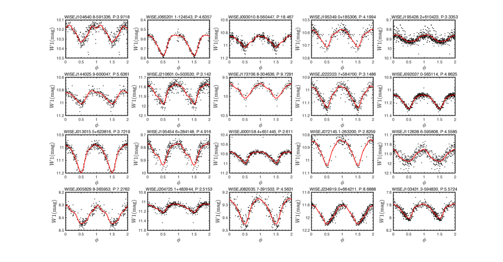
Figure 10: Light curve examples for 20 of the new Cepheids. The black dots and red line are the observed and best-fitting light curves, respectively. The full set of light curves is available online.

Classical Cepheids are the most important and among the most accurate distance indicators used for establishing the astronomical distance scale. Compared with extragalactic Cepheids, Cepheids in our Galaxy are poorly detected. Some 500 of Cepheids with good photometry were listed by Berdnikov et al. (2008). Around 800 Cep-Is are included in the ASAS catalog (Pojmanski et al., 2005). However, contamination of the sample is a problem. To date, only 450 Cepheids are usually used to study Galactic structure (Genovali et al., 2014). Note that these Cepheids are predominantly located in the solar neighborhood. Because of the heavy reddening and crowded environment in the inner plane, only a few to a few dozen Cepheids have been found there (e.g. Matsunaga et al., 2013, 2015; Dékány et al., 2015; Tanioka et al., 2017; Inno et al., 2018). Here, we report 1312 newly discovered Cepheids; the majority are classical Cepheids in the inner plane. This should promote a significantly better understanding of the inner plane’s structure. The huge increase of Galactic Cepheids also offers the possibility to better constrain the scatter and zeropoint of the Cepheid period–luminosity relation (PLR). In addition, Cepheids are usually associated with young open clusters or OB associations. Finding new open cluster Cepheids is valuable (Chen et al., 2015, 2017; Lohr et al., 2018), since it may help us understand the evolution of intermediate-mass stars (Smiljanic et al, 2018). Figure 10 shows 20 randomly selected Cepheid light curves. Our Cepheid sample is contaminated by roughly 10% of objects that are actually eclipsing binaries, rotating stars, and long-period quasi-periodic variables; their nature should be double checked based on their color, extinction, and distance properties.

6.2 RR Lyrae

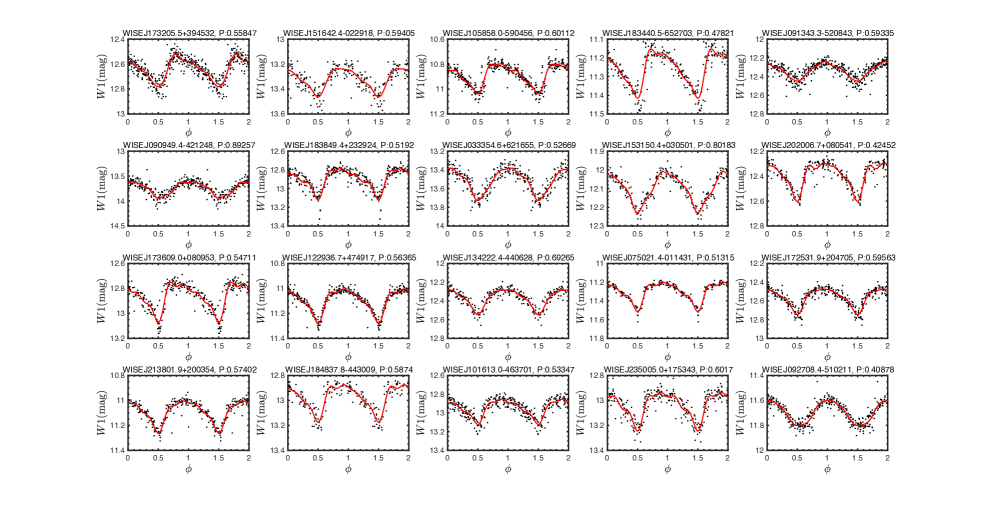
Figure 11: Example light curves of 20 new RR Lyreas. The black dots and red line are the observed and best-fitting light curves, respectively. The full set of light curves is available online.

RR Lyrae comprise another useful distance indicator that could trace old environments with 4–5% distance accuracy (Catelan et al., 2009, and references within). They are advantageous to study the Galactic halo (Vivas & Zinn, 2006; Sesar et al, 2010; Drake et al., 2013), bulge (Gran et al., 2016), as well as the solar neighborhood (Layden, 1994, 1998). The 1231 newly discovered RR Lyrae in our catalog expand the number of known RR Lyrae in the solar neighborhood, especially in reddened regions. Figure 11 shows example light curves of new RR Lyrae. In this period range, 6% of misidentified eclipsing binaries are hard to exclude only based on their light curves. Colors, independent distances, or amplitudes in optical bands would be helpful to improve the sample’s purity.

6.3 Eclipsing binaries

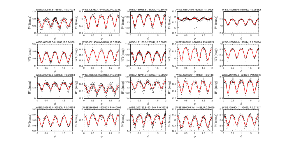
Figure 12: Example light curves of 20 new EW. The black dots and red line are the observed and best-fitting light curves, respectively. The full set of light curves is available online.

Eclipsing binaries are among the most plentiful variables in the periodic variable catalog. Based on their light curves, they are divided into three subtypes: EA, EB, and EW type refer to detached, semi-detached, and contact binaries. The majority of EW types are over-contact, contact, or near-contact eclipsing binaries, which follow the relevant PLR in some period range. In particular, W UMa-type contact binaries in the period range 0.25–0.56 days are important distance indicators. Chen et al. (2018) established their PLRs based on Gaia DR1 parallaxes (Gaia Collaboration, 2016). They could be used to trace distances to an accuracy of 7–8% in $W1$ band. With the updated Gaia DR2 parallaxes, the accuracy could be improved to 6% (0.13 mag) in the $W1$ band. Chen et al. (2018) also studied the structure of the solar neighborhood based on more than 20,000 W UMa-type contact binaries from the Catalina and ASAS catalogs. However, the Galactic plane was not covered. The 20,000 newly discovered EW-type eclipsing binaries fill in the Galactic plane and allow us to construct a complete sample covering distances out to 2–3 kpc from the Sun. Figure 12 shows example light curves of EW-type eclipsing binaries.

Figure 13: Example light curves of 20 new EA-type binaries. The black dots and red line are the observed and best-fitting light curves. The full set of light curves is available online.

Compared to EW, it is easy to identify the eclipse onset in EA light curves (see Figure 13). The majority of EAs are detached eclipsing binaries. Combining the light and radial velocity curves, detached eclipsing binaries are the best objects one can use to determine stellar parameters and accurate distances (Grundahl et al., 2008; Pietrzynski et al., 2013).

7 Conclusions

In this paper, we have collected five-year ALLWISE and NEOWISE-R data to detect periodic variables. Based on 2.7 million high-probability candidates in ALLWISE, we found 50,282 periodic variables and an additional 17,000 suspected variables. With more than 100 detections each, these variables represent a well-observed catalog. A global variable classification scheme based on $W1$-band light curves was established and the first all-sky infrared variable star catalog was constructed. Among the catalog’s 50,282 periodic variables, 34,769 are newly discovered, including 21,427 EW-type eclipsing binaries, 5654 EA-type eclipsing binaries, 1312 Cepheids, and 1231 RR Lyrae. The newly found variables are located in the Galactic plane and the equatorial poles, which where were not well covered in earlier studies. Since the $W1$-band extinction is one-twentieth of that in the $V$ band, these variables can be used to pierce through the heavy dust in the Galactic plane. A careful parameter double check with the literature for the reconfirmed variables was done, resulting in misclassification rates of 5% and 10%, respectively, for short- and long-period variables. Type, period, and amplitude comparisons with the Catalina catalog not only validated our sample of variables, but also implied different optical–infrared properties for different types of variables.

The newly found variables can be used to trace new structures or better study the Galactic plane, the spiral arms, and the solar neighborhood. Especially for Cepheids, the number of known objects has increased by an order of magnitude in the inner plane. The scatter, zero point, and systematics of Cepheid, RR Lyrae, and W UMa-type contact-binary PLRs will also benefit from this expanded sample. These objects are helpful to study stellar evolution based on a more complete sample. In addition, based on some variables located in heavily reddened regions, the infrared extinction law may be better characterized. To avoid the detection of false positives, these 50,282 variables are highly selected variables with completeness levels in excess of 50%. WISE operations are continuing, and an additional 30,000 variables are expected to be found based on the enhanced data. These MIR variables are also interesting candidates for future targeted campaigns with the James Webb Space Telescope.

References

- Akerlof et al. (2000) Akerlof, C., Amrose, S., Balsano, R., et al. 2000, AJ, 119, 1901
- Alcock et al. (1993) Alcock, C., Akerlof, C. W., Allsman, R. A., et al. 1993, Natur, 365, 621
- Bhardwaj et al. (2017) Bhardwaj, A., Macri, L. M., Rejkuba, M., et al. 2017, AJ, 153, 154
- Berdnikov et al. (2008) Berdnikov, L. N. 2008, VizieR On-line Data Catalog: II/285
- Catelan et al. (2009) Catelan, M. 2009, Ap&SS, 320, 261
- Cutri et al. (2003) Cutri R. M. et al., 2003, The 2MASS Catalogue of Point Sources. Univ. Massachusetts & IPAC/Caltech
- Chen et al. (2015) Chen, X., de Grijs, R., Deng, L., 2015, MNRAS, 446, 1268
- Chen et al. (2016) Chen, X., de Grijs, R., Deng, L., 2016, ApJ, 832, 138
- Chen et al. (2017) Chen, X., de Grijs, R., Deng, L., 2017, MNRAS, 464, 1119
- Chen et al. (2018) Chen, X., Deng, L., de Grijs, R., Wang, S., & Feng, Y., 2018a, ApJ, 859, 140
- Chen et al. (2018) Chen, X., Wang, S., Deng, L., & de Grijs, R., 2018b, ApJ, 859, 137
- Clementini et al. (2018) Clementini, G., Ripepi, V., Molinaro, R. et al., 2018, A&A, submitted (arXiv:1805.02079)
- Dékány et al. (2015) Dékány, I., Minniti, D., Majaess, D., et al. 2015, ApJL, 812, L29
- Drake et al. (2013) Drake, A. J., Catelan, M., Djorgovski, S. G., et al., 2013, ApJ, 763, 32
- Drake et al. (2014) Drake, A. J., Graham, M. J., Djorgovski, S. G., el al. 2014, ApJS, 213, 9
- Drake et al. (2017) Drake, A. J., Djorgovski, S. G., Catelan, M., et al. 2017, MNRAS, 469, 3688
- Feast et al. (2014) Feast, M. W., Menzies, J. W., Matsunaga, N., Whitelock, P. A., 2014, Natur, 509, 342
- Flaherty et al. (2007) Flaherty, K. M., Pipher, J. L., Megeath, S. T., et al. 2007, ApJ, 663, 1069
- Gaia Collaboration (2016) Gaia Collaboration, Brown, A. G. A., Vallenari, A., et al. 2016, A&A, 595, A2
- Gaia Collaboration (2017) Gaia Collaboration, Clementini, G., Eyer, L., et al. 2017, A&A, 605, A79
- Gavrilchenko et al (2014) Gavrilchenko, T., Klein, C. R., Bloom, J. S., & Richards, J. W. 2014, MNRAS, 441, 715
- Genovali et al. (2014) Genovali, K., Lemasle, B., Bono, G., et al. 2014, A&A, 566, A37
- Gran et al. (2016) Gran, F., Minniti, D., Saito, R. K., et al. 2016, A&A, 591, A145
- Grundahl et al. (2008) Grundahl, F., Clausen, J. V., Hardis, S., & Frandsen, S. 2008, A&A, 492, 171
- Hoffman et al. (2009) Hoffman, D. I., Harrison, T. E., McNamara, B. J., 2009, AJ, 138, 466
- Inno et al. (2015) Inno, L., Matsunaga, N., Romaniello, M., et al. 2015, A&A, 576, A30
- Inno et al. (2016) Inno, L., Bono, G., Matsunaga, N., et al. 2016, ApJ, 832, 176
- Inno et al. (2018) Inno, L., Urbaneja, M. A., Matsunaga, N., et al. 2018, MNRAS, submitted (arXiv:1805.03212)
- Jones et al. (1996) Jones, R. V., Carney, B. W., & Fulbright, J. P. 1996, PASP, 108, 877
- Layden (1994) Layden, A. C. 1994, AJ, 108, 1016
- Layden (1998) Layden, A. C. 1998, AJ, 115, 193
- Lohr et al. (2018) Lohr, M. E., Negueruela, I., Tabernero, H. M., et al. 2018, MNRAS, 478, 3825
- Lomb (1976) Lomb, N. R. 1976, Ap&SS, 39, 447
- Mainzer et al. (2011) Mainzer, A., Bauer, J., Grav, T., et al. 2011, ApJ, 731, 53
- Mainzer et al. (2014) Mainzer, A., Bauer, J., Cutri, R. M., et al. 2014, ApJ, 792, 30
- Matsunaga et al. (2011) Matsunaga N., Kawadu, T., Nishiyama, S., et al., 2011, Natur, 477, 188
- Matsunaga et al. (2013) Matsunaga, N., Feast, M. W., Kawadu, T., et al. 2013, MNRAS, 429, 385
- Matsunaga et al. (2015) Matsunaga, N., Fukue, K., Yamamoto, R., et al., 2015, ApJ, 799, 46
- Matsunaga et al. (2018) Matsunaga, N., Bono, G., Chen, X., et al., 2018, Space Sci Rev, 214, 74
- Minniti et al. (2010) Minniti, D., Lucas, P. W., Emerson, J. P., et al. 2010, NewA, 15, 433
- Minniti et al. (2017) Minniti, D., Dékány, I., Majaess, D., et al., 2017, AJ, 153, 179
- Palaversa et al. (2013) Palaversa, L., Ivezić, Ž., Eyer, L., et al. 2013, AJ, 146, 101
- Pietrzynski et al. (2013) Pietrzyński, G., Graczyk, D., Gieren, W., et al. 2013, Natur, 495, 76
- Pojmanski et al. (1997) Pojmanski, G., 1997, Acta Astron., 47, 467
- Pojmanski et al. (2005) Pojmanski, G., Pilecki, B., & Szczygiel, D. 2005, AcA, 55, 275
- Scargle (1982) Scargle, J. D. 1982, ApJ, 263, 835
- Sesar et al (2010) Sesar, B., Ivezić, Ž., Grammer, S. H., et al. 2010, ApJ, 708, 717
- Sesar et al (2011) Sesar, B., Stuart, J. S., Ivezić, Ž., et al. 2011, AJ, 142, 190
- Smiljanic et al (2018) Smiljanic, R., Donati, P., Bragaglia, A., Lemasle, B., Romano, D. 2018, A&A, in press (arXiv:1805.03460)
- Soszynski et al. (2008a) Soszyński, I., Poleski, R., Udalski, A., et al., 2008a, Acta Astron., 58, 163
- Soszynski et al. (2008b) Soszyński, I., Udalski, A., Szymański, M. K., et al., 2008b, Acta Astron., 58, 293
- Soszynski et al. (2009) Soszyński I., Udalski, A., Szymański, M. K., et al., 2009, Acta Astron., 59, 1
- Tanioka et al. (2017) Tanioka S., Matsunaga N., Fukue K., et al., 2017, ApJ, 842, 104
- Udalski et al. (1994) Udalski, A., Szymański, M., Kaluzny, J., et al. 1994, ApJ, 426, 69
- Udalski et al. (2015) Udalski, A., Szymański, M. K., Szymański, G., 2015, Acta Astron., 65, 1
- Vivas & Zinn (2006) Vivas, A. K., & Zinn, R. 2006, AJ, 132, 714
- Wang & Jiang (2014) Wang, S., & Jiang, B. W. 2014, ApJ, 788, L12
- Wang et al. (2018) Wang, S., Chen, X. D., de Grijs, R., Deng, L. 2018, ApJ, 852, 78
- Wright et al. (2010) Wright, E. L., Eisenhardt, P. R. M., Mainzer, A. K., et al. 2010, AJ, 140, 1868
- Wozniak et al. (2004) Wozńiak, P. R., Williams, S. J., Vestrand, W. T., Gupta, V., 2004, AJ, 127, 2436
- Zasowski et al. (2009) Zasowski, G., Majewski, S. R., Indebetouw, R., et al. 2009, ApJ, 707, 510