Extraction of the Specific Shear Viscosity of Hot Hadron Gas

Abstract

We extract the specific shear viscosity $\eta/s$ of nuclear matter for various temperatures and chemical potentials in the hadronic phase using data taken in high energy nuclear collisions. We use a blastwave parameterization of the final state of nuclear collisions, including non-equilibrium deformations of particle distributions due to shear stress in the Navier-Stokes approximation. We fit spectra and elliptic flow of identified hadrons for a variety of collision energies and impact parameters at the Relativistic Heavy Ion Collider (RHIC) and the Large Hadron Collider (LHC). The systems analyzed cover a temperature range from about 110 to 140 MeV and vary in their chemical potentials for stable hadrons. We attempt to assign meaningful systematic uncertainties to our results. This work is complementary to efforts using viscous fluid dynamics to extract the specific shear viscosity of quark gluon plasma at higher temperatures. We put our work in context with existing theoretical calculations of the specific shear viscosity.

I Introduction

Quark gluon plasma (QGP) and hot hadron gas are routinely created in nuclear collisions at the Relativistic Heavy Ion Collider (RHIC) and the Large Hadron Collider (LHC). Soon after the start of the RHIC program it was realized that experimental data from this machine required a new paradigm. Although the original motivation for postulating the existence of quark gluon plasma came from the known weakening of the strong coupling constant with temperature Collins:1974ky ; Shuryak:1978ij , it turned out that QGP close to the pseudo-critical temperature $T_{c}$, i.e. at temperatures probed by the experimental programs at RHIC and LHC, rather behaves like a strongly coupled liquid Gyulassy:2004zy ; Shuryak:2008eq . The first hint came from the great success enjoyed by ideal fluid dynamics in describing the flow of hadrons measured at RHIC Kolb:2000fha ; Huovinen:2001cy . As it turns out, the process of cooling and expansion of the fireball of QGP and hadron gas behaves hydrodynamically from very early times in the collision onward. Subsequently, relativistic viscous fluid dynamic simulations compared to data allowed the quantitative extraction of $\eta/s$ from data Romatschke:2007mq ; Dusling:2007gi ; Schenke:2011tv ; Heinz:2013th . Around the same time, Kovtun, Son and Starinets hypothesized that there might be a universal lower bound of $\eta/s=1/(4\pi)$ for the specific shear viscosity, based on their study of strongly interacting systems using AdS/CFT correspondence Kovtun:2004de . Quark gluon plasma quickly became a celebrated example of an ideal liquid.

Measurements of the specific shear viscosity $\eta/s$ utilize viscous fluid dynamic simulations compared to experimental data. Collective flow observables are particularly sensitive to shear viscosity. The first generation of calculations used relativistic fluid dynamics with a fixed, temperature-independent $\eta/s$ as a parameter. Fluid dynamics was run all the way to kinetic freeze-out in the hadronic phase which was modeled very similar to the approach discussed further below here. Obviously the value of $\eta/s$ extracted from this method is averaged over the entire temperature evolution of the QGP and the hot hadron gas below $T_{c}$, a range of several hundred MeV at top RHIC and LHC energies. $\eta/s$ extracted through this method also includes the effects of deformations of particle distributions at freeze-out that are present at finite shear stress Teaney:2003kp ; Dusling:2007gi .

Subsequently, several groups argued that the hadronic phase should be rather described by hadronic transport models because the specific shear viscosity in the hadronic phase could be too large for the evolution to be described accurately in second order viscous fluid dynamic codes Song:2010aq ; Song:2011hk . This argument was aided by estimates of $\eta/s$ for hadron gas from chiral perturbation theory, effective theories and hadronic transport by various groups Prakash:1993bt ; Muroya:2004pu ; Dobado:2003wr ; Chen:2006iga ; Itakura:2007mx ; Dobado:2008vt ; Demir:2008tr ; FernandezFraile:2009mi ; Romatschke:2014gna ; Rose:2017bjz . While these calculations do not agree quantitatively, they generally find rather large specific shear viscosity for a hot hadron gas, $\eta/s\gtrsim 4/(4\pi)$ even very close to $T_{c}$, see Fig. 8. Thus fluid dynamic calculations were matched to hadronic transport models just below $T_{c}$ while $\eta/s$ was retained as a parameter only for the QGP phase and the crossover region around $T_{c}$. Even more recently, fluid dynamic calculations using simple parameterizations have also been used to constrain the functional form of the temperature dependence of $\eta/s$, mostly for the QGP case Song:2010aq ; Niemi:2012ry ; Bernhard:2015hxa . We refer the reader to Gale:2013da ; Heinz:2013th ; Romatschke:2017ejr for reviews of fluid dynamic simulations of nuclear collisions, including the extraction of shear viscosity.

Lattice calculations of $\eta/s$ in the QGP phase have been attempted but are challenging Meyer:2007ic ; Meyer:2009jp ; Haas:2013hpa ; Mages:2015rea ; Astrakhantsev:2017nrs . They generally find $\eta/s$ to be close to the conjectured lower bound around $T_{c}$ with a rather slow rise towards higher temperatures. Perturbative QCD calculations at leading order have indicated large values of $\eta/s$ at temperatures well above $T_{c}$ Arnold:2000dr ; Arnold:2003zc , but a recent next-to-leading order calculation predicts a significant drop towards $T_{c}$ which makes the perturbative results comparable to lattice QCD Ghiglieri:2018dib .

From general arguments one expects a minimum of $\eta/s$ around $T_{c}$ which has been found to be the case for a large variety of systems Csernai:2006zz . How fast the specific shear viscosity is rising towards lower temperatures below $T_{c}$ can not be seen as settled from either data nor first principle calculations. Features should be continuous as a function of temperature but could be changing quickly. Progress has been made in undestanding the large values of $\eta/s$ in hadronic transport Rose:2017bjz . However, these effective theories mostly do not incorporate the existence of a pseudo-critical temperature and their predictions close to this temperature should be viewed with caution. The question of the specific shear viscosity of hadron gas is an important one. In any conceivable experiment information on specific shear viscosity in the QGP phase is always convoluted with contributions from the hadronic phase. Thus uncertainties in hadronic $\eta/s$ are directly responsible for increased uncertainties of QGP shear viscosities extracted from data.

It is clear that an independent assessment of the hadronic specific shear viscosity is necessary to improve the situation. As a reasonable minimum requirement, theoretical uncertainties coming from incomplete knowledge of the hadronic phase should inform realistic contributions to error bars for quantities extracted for the QGP phase. For this reason we attempt a realistic uncertainty estimate in this work, Moreover, the specific shear viscosity of a hot hadron gas is by itself a compelling question.

Here, we argue that it is possible to use experimental data to estimate the specific shear viscosity of the hot hadron gas at the kinetic freeze-out independently. The main effect of the time evolution of the system before freeze-out is the build-up of a flow field $u^{\mu}$ which leads to the system expanding and cooling. Viscous corrections to first order are given by gradients of the flow field (Navier-Stokes approximation). Computing the flow field in fluid dynamics, introduces additional dependences on initial conditions and the equation of state. We take a complementary approach and fit the final flow field, together with the temperature and system size at kinetic freeze-out. The specific shear viscosity is then a parameter at just one fixed temperature $T=T_{\mathrm{fo}}$, the kinetic freeze-out temperature, and a set of chemical potentials ${\mathbf{\mu}}_{\mathrm{fo}}=(\mu_{B},\mu_{\pi},\ldots)$ for baryon number $B$, and abundances of stable hadrons like pions, kaons and nucleons. Of course, such fits of flow fields and temperatures at freeze-out are well established and generally known as blastwave parameterizations Westfall:1976fu ; Schnedermann:1993ws ; Retiere:2003kf . We will use such a blastwave, with $\eta/s$ added as a parameter, to extract $\eta/s(T_{\mathrm{fo}},{\mathbf{\mu}}_{\mathrm{fo}})$ for a variety of points ($T_{\mathrm{fo}}$,${\mathbf{\mu}}_{\mathrm{fo}}$) in different collision systems. Here we present the results for Au+Au collisions at top RHIC energies and Pb+Pb collisions at LHC where the baryon chemical potential vanishes $\mu_{B}\approx 0$. However, non-vanishing chemical potentials $\mu_{\pi}$, $\mu_{K}$ and $\mu_{p}$ are present at kinetic freeze-out, determined by the chemical freeze-out at higher temperatures. Our extraction is complementary to fluid dynamics, which integrates over the effects of shear viscosity over a wide temperature range. Some of the uncertainties in both approaches are the same. For example the assumption of a sharp kinetic freeze-out at a fixed temperature is common to both approaches and is only an approximation, although it can be improved in the case of fluid dynamics by matching to hadronic transport. Other uncertainties are different in both approaches. For example the dependence of fluid dynamic calculations on initial conditions, which themselves are not well constrained experimentally, is not present in our approach. We will discuss uncertainties in the blastwave extraction in more detail below. This paper is organized as follows: In section 2 we present our blastwave parameterization, especially the viscous correction term. In section 3 we discuss the simulation and data selection. In section 4 we show fit results and carry out an analysis of uncertainties. We conclude with a discussion and outlook in section 5.

II A Viscous Blast Wave

Viscous corrections to blastwaves have been studied in Teaney:2003kp ; Jaiswal:2015saa . Both of these previous works assume spatial spherical symmetry in the transverse plane and free streaming for simplicity. We will generalize these assumptions here. We choose the blastwave of Retiere and Lisa (RL) Retiere:2003kf as our starting point. In this section we discuss the Retiere-Lisa blastwave and compute the Navier-Stokes corrections.

We have to make two major assumptions in our analysis, both of which have been routinely used and studied in the literature. The first is that at freeze-out the system of hadrons is close enough to kinetic equilibrium so that at any position $r^{\mu}=(t,x,y,z)$ there exist a local rest frame with a local temperature $T_{\mathrm{fo}}(r)$ and a set of chemical potentials ${\mathbf{\mu}}_{\mathrm{fo}}(r)$ such that the particle distribution in the local rest frame can be written as

$$f(r,p)=f_{0}(r,p)+\delta f(r,p)$$ (1)

where $f_{0}$ is the equilibrium Bose/Fermi-distribution with the local temperature and chemical potentials,

$$f_{0}(r,p)=\frac{1}{e^{(E-\mu(r,p))/T_{\mathrm{fo}}(r,p)}\mp 1}\,,$$ (2)

and $\delta f$ is a gradient correction of Navier-Stokes type. Here we use the general form

$$\delta f(r,p)=\frac{\eta}{s}\frac{\Gamma(6)}{\Gamma(4+\lambda)}\left(\frac{E}{T_{\mathrm{fo}}}\right)^{2-\lambda}\frac{p^{\mu}p^{\nu}}{T_{\mathrm{fo}}^{3}}\sigma^{\mu\nu}f_{0}(r,p)$$ (3)

which follows from a generalized Grad ansatz Damodaran:2017ior . In the Navier-Stokes approximation the viscous correction is proportional to the traceless shear gradient tensor, defined as

$$\sigma^{\mu\nu}=\frac{1}{2}\left(\nabla^{\mu}u^{\nu}+\nabla^{\nu}u^{\mu}\right)-\frac{1}{3}\Delta^{\mu\nu}\nabla_{\lambda}u^{\lambda}\,.$$ (4)

Here $\nabla^{\mu}=\Delta^{\mu\nu}\partial_{\nu}$, with $\Delta^{\mu\nu}=g^{\mu\nu}-u^{\mu}u^{\nu}$, is the derivative perpendicular to the flow field vector $u^{\mu}$. The gradient corrections need to be small and we will ensure that numerically $\delta f\lesssim f$ for all relevant momenta in this analysis. The power $\lambda$ parameterizes further details of the underlying microscopic physics. Here we restrict ourselves to the original Grad ansatz $\lambda=2$ which is widely used. We reserve a more detailed analysis including $\lambda$ as a tunable parameter for future work.

The second major assumption in our analysis pertains to the simplified shape of the freeze-out hypersurface and flow field. In longitudinal direction (along the colliding beams) we assume boost-invariance, which is a good approximation for particles measured around midrapidity at LHC and top RHIC energies. Blast wave parameterizations assume that freeze-out happens at constant $T_{\mathrm{fo}}$ and ${\mathbf{\mu}}_{\mathrm{fo}}$ which is approximated by a constant (longitudinal) proper time $\tau=\tau_{\mathrm{fo}}$. In the RL parameterization the transverse shape of the fireball at freeze-out is assumed to be an ellipse with semi axes $R_{x}$ and $R_{y}$ in $x$- and $y$-directions respectively. We define the coordinate axes such that the impact parameter $b$ of the collision is measured along the $x$-axis. In the following we use the reduced radius $\rho=\sqrt{x^{2}/R_{x}^{2}+y^{2}/R_{y}^{2}}$. The flow field can be parameterized as

$$u^{\mu}=\left(\cosh\eta_{s}\cosh\eta_{T},\sinh\eta_{T}\cos\phi_{u},\sinh\eta_{T}\sin\phi_{u},\sinh\eta_{s}\cosh\eta_{T}\right)$$ (5)

where $\eta_{T}$ is the transverse rapidity in the $x-y$-plane, and $\phi_{u}$ is the azimuthal angle of the flow vector in the transverse plane. Boost invariance fixes the longitudinal flow rapidity to be equal to the space time rapidity $\eta_{s}=1/2\log[(t+z)/(t-z)]$. For the transverse flow velocity $v_{T}=\tanh\eta_{T}$ we make the assumption Retiere:2003kf

$$v_{T}=\rho^{n}\left(\alpha_{0}+\alpha_{2}\cos(2\phi_{u})\right)$$ (6)

which encodes a Hubble-like velocity ordering with an additional shape parameter $n$. $\alpha_{0}$ is the average velocity on the boundary $\rho=1$, and $\alpha_{2}$ parameterizes an elliptic deformation of the flow field coming from the original elliptic spatial deformation of systems with finite impact parameters. The time evolution of pressure gradients in the expansion leads to flow vectors tilted towards the smaller axis of the ellipse. This is accomplished by demanding that the transverse flow vector is perpendicular to the elliptic surface at $\rho=1$, i.e. $\tan\phi_{u}=R_{x}^{2}/R_{y}^{2}\tan\phi$, where $\phi=\arctan y/x$ is the azimuthal angle of the position $r^{\mu}$. Higher order deformations could be present Jaiswal:2015saa , but the two main observables chosen for our analysis are not particularly sensitive to them.

Using the assumptions laid out here we can write the spectrum of hadrons emitted from freeze-out as Cooper:1974mv

$$\frac{dN}{dyd^{2}P_{T}}=g\int\frac{p\cdot d\Sigma}{(2\pi)^{3}}f(r,u\cdot p)$$ (7)

where $g$ is the degeneracy factor for a given hadron. The momentum vector in the laboratory frame is written in standard form as $p^{\mu}=(M_{T}\cosh y,P_{T}\cos\psi,$ $P_{T}\sin\psi,M_{T}\sinh y)$ in terms of the transverse momentum $P_{T}$, the longitudinal momentum rapidity $y$ and the azimuthal angle $\psi$ in the transverse plane. $M_{T}^{2}=P_{T}^{2}+M^{2}$ defines the transverse mass $M_{T}$ for a hadron of mass $M$. $d\Sigma^{\mu}$ is a parameterization of the $T=T_{\mathrm{fo}}$ hypersurface and its outbound normal vector. With our assumptions we have $d\Sigma^{\mu}=\tau_{\mathrm{fo}}R_{x}R_{y}d\eta_{s}\rho d\rho d\theta(\cosh\eta_{s},0,0,\sinh\eta_{s})$. Hence, for hadrons measured around midrapidity ($y=0$) the spectrum takes the standard form

$$\frac{dN}{dyd^{2}P_{T}}=g\tau_{\mathrm{fo}}R_{x}R_{y}M_{T}\int_{0}^{1}d\rho\int_{0}^{2\pi}d\theta\int_{-\infty}^{\infty}d\eta_{s}\frac{\rho\cosh\eta_{s}}{(2\pi)^{3}}f_{0}(\rho,\theta,\eta_{s};u\cdot p)\left[1+\frac{\eta}{s}\frac{1}{T_{\mathrm{fo}}^{3}}p^{\mu}p^{\nu}\sigma^{\mu\nu}\right]$$ (8)

where $\tan\theta=R_{x}/R_{y}\tan\phi$. The set of parameters in this ansatz is $\tilde{\mathcal{P}}=(\tau_{\mathrm{fo}},R_{x},R_{y},T_{\mathrm{fo}},{\mathbf{\mu}}_{\mathrm{fo}},n,\alpha_{0},\alpha_{2},\eta/s)$.

We can now determine the shear gradient tensor $\sigma^{\mu\nu}$ for the RL blastwave, following the example of Teaney:2003kp ; Jaiswal:2015saa . Without azimuthal symmetry the spatial derivatives in $\sigma^{\mu\nu}$ are still straight forward to obtain, starting from the explicit expression in Eq. (5), but the results are somewhat lengthy. We delegate a discussion of details of these expressions to another work. The task of determining the time-derivatives in $\sigma^{\mu\nu}$ can be reduced to the question of computing $\partial_{\tau}\eta_{T}$ and $\partial_{\tau}\phi_{u}$. We start from the relativistic fluid dynamic equations of motion $\partial_{\mu}T^{\mu\nu}=0$, where $T^{\mu\nu}=eu^{\mu}u^{\nu}-p\Delta^{\mu\nu}$ is the ideal energy momentum tensor. We can restrict ourselves to ideal fluid dynamics to obtain the leading order expressions in a gradient expansion for the time derivatives. Dissipative corrections in the determination of the time derivatives would lead to terms of order $\eta^{2}\times\text{(second order spatial gradients)}$ in $\delta f$ which we neglect. Here $e$ is the local energy density and $p$ the pressure. The ideal fluid dynamics equations can be rewritten more instructively as the set of equations

$$De= -(e+p)\partial_{\mu}u^{\mu}=-(e+p)\nabla_{\mu}u^{\mu}$$ (9)

$$Du^{\mu}= \frac{\nabla^{\mu}p}{e+p}$$ (10)

where the co-moving time derivative is $D=u_{\mu}\partial^{\mu}$.

Freeze-out is the process of decoupling of particles where the mean free path rapidly grows beyond the system size. In fluid dynamics this process is modeled through a sudden transition during which the mean free path goes from very small values to infinity instantaneously at $T=T_{\mathrm{fo}}$. The system is free streaming, $Du^{\mu}=0$, after the transition, i.e. from $T=T_{\mathrm{fo}}-\epsilon$ on (with small $\epsilon>0$). Thus the assumption of free streaming has been used in some previous work on viscous blastwaves Teaney:2003kp ; Jaiswal:2015saa . However, it seems more physical to assume that the local particle distributions $f(r,p)$ remain frozen across the $T=T_{\mathrm{fo}}$ hypersurface and that $\sigma^{\mu\nu}$, including time derivatives, should be set at temperature $T=T_{\mathrm{fo}}+\epsilon$. This is consistent with the treatment in fluid dynamics. Eqs. (9), (10) can be solved for the blast wave geometry and flow field assumed here to obtain the time derivatives we seek.

Using (9) together with the first or fourth equation ($\mu=0,3$; the two equations are equivalent) in (10) we obtain the time derivative of the transverse flow rapidity,

$$(1-c_{s}^{2}\tanh^{2}\eta_{T})\partial_{\tau}\cosh\eta_{T}=c_{s}^{2}\tanh^{2}\eta_{T}(\partial_{1}u^{1}+\partial_{2}u^{2}+\frac{\cosh\eta_{T}}{\tau})-\frac{u^{1}\partial_{1}u^{0}}{u^{0}}-\frac{u^{2}\partial_{2}u^{0}}{u^{0}}\,,$$ (11)

in terms of known spatial derivatives. $c_{s}^{2}=\partial p/\partial e$ is the speed of sound squared, given by the equation of state of the system at $T=T_{\mathrm{fo}}$. The time derivative of the direction of the transverse flow field can be computed by using (11) in the second and third equation ($\mu=1,2$) in (10).

This completes the brief introduction of the blastwave model used in our analysis. We can in principle validate the blastwave by comparison with established fluid dynamics calculations. Here we will use the viscous fluid code MUSIC Schenke:2010nt ; Ryu:2015vwa for this purpose. Since the blastwave, for simplicity, ignores the effects of feed-down from hadronic resonances as well as bulk stress, we can quantify the uncertainty and bias from these simplifications by comparing to MUSIC calculations with resonance decays and bulk stress included. This comparison is important to estimate uncertainties in the extraction of $\eta/s$ and will be discussed in some detail below.

Centrality	proton (GeV/$c$)	kaon (GeV/$c$)	pion (GeV/$c$)	$b$ (fm)	$c_{s}^{2}$	$c_{\tau}$
ALICE 2.76 TeV
10-20%	0.325-3.3	0.225-2.55	0.525-1.85	6.05	0.158	0.783
20-30%	0.325-3.1	0.225-2.35	0.525-1.75	7.81	0.162	0.756
30-40%	0.325-3.1	0.225-2.25	0.525-1.65	9.23	0.166	0.720
40-50%	0.325-2.95	0.225-2.15	0.525-1.45	10.47	0.170	0.679
50-60%	0.325-2.55	0.225-1.85	0.525-1.25	11.58	0.174	0.633
PHENIX 0.2 TeV
10-20%	0.55-2.9	0.55-1.85	0.55-1.65	5.70	0.164	0.780
20-40%	0.55-2.7	0.55-1.75	0.55-1.55	8.10 (7.4, 8.7)	0.170	0.739
40-60%	0.55-2.5	0.55-1.65	0.55-1.45	10.5 (9.9, 11,0)	0.178	0.660
MUSIC 0.2 TeV
spectra ($v_{2}$)	0.25-2.34 (3.0)	0.31-2.0 (3.0)	0.38-1.77 (3.0)	7.5	0.178	0.60

Table 1: Regular fit range (RFR) selected for each ALICE and PHENIX centrality bin for the spectra of all three particle species. The bins for elliptic flow data are chosen consistently. We also show the average impact parameter $b$ from Glauber Monte Carlo calculations quoted by the experiments, the speed of sound squared $c_{s}^{2}$ and the expansion parameter $c_{\tau}$ determined for each data set. For PHENIX data the average impact parameter for the two 10% bins included in a given 20 % bin are quoted in parentheses. The bottom part of the table shows out choice of fit range for the spectra obtained from the MUSIC hydro code, see Sec. IV. MUSIC $v_{2}$ output is fit up to 3 GeV/$c$.

III Simulation and Data Selection

With $\sigma^{\mu\nu}$ known it is straightforward to evaluate Eq. (8) numerically, dependent on the set of parameters $\tilde{\mathcal{P}}$ which can be determined from the fits to data or other methods. We carry out this analysis using data on identified protons and antiprotons, kaons and pions from LHC and RHIC. We utilize both transverse momentum spectra around mid-rapidity, and elliptic flow $v_{2}$, the leading harmonic deformation of the spectrum in azimuthal momentum space angle $\psi$, as functions of hadron transverse momentum $P_{T}$. They are calculated from (8) as

$$\frac{dN}{2\pi P_{T}dP_{T}dy} =\frac{1}{2\pi}\int d\psi\frac{dN}{dyd^{2}P_{T}}\,,$$ (12)

$$v_{2}(P_{T}) ={\left(\frac{dN}{2\pi P_{T}dP_{T}dy}\right)}^{-1}\frac{1}{2\pi}\int d\psi\cos(2\psi)\frac{dN}{dyd^{2}P_{T}}\,,$$ (13)

respectively. Note that the blastwave does not incorporate fluctuations. This is one reason why we will not analyze the most central and peripheral centrality bins available which are known to exhibit large effects due to fluctuations. All expressions in the blast wave are taken at rapidity $y=0$ and we have utilized matching data sets that have been taken around midrapidity.

We use data from the ALICE collaboration for Pb+Pb collisions at 2.76 TeV Adam:2015kca ; Abelev:2014pua , in 10% centrality bins, and from the PHENIX collaboration for Au+Au collisions at 200 GeV Adare:2013esx ; Adare:2014kci . The PHENIX data is binned in 10 or 20% centrality bins for the spectra and 10% centrality bins for elliptic flow. For this analysis, if the PHENIX spectrum is only availabe in a coarser bin we combine a given 10% bin for elliptic flow together with the overlapping 20% bin for the spectrum. We find that centralities that share the coarser spectrum bins give results for temperature and specific shear viscosity that agree very well with each other within estimated uncertainties.

The selection of data points for the fit can introduce a bias that we try to quantify as an uncertainty. The following general principles were applied in the selection. We expect the blastwave parameterization to extract inaccurate parameters at too low momenta where resonance decays dominate the spectrum Sollfrank:1991xm . We also expect it to fail at too large momentum where gradient corrections become large, and hadrons from other production channels, like hard processes, start to dominate soft particles from the bulk of the fireball. The maximum momentum $P_{T}$ described by the blastwave increases from peripheral to more central collisions, since particles are expected to be more thermalized when volumes and lifetimes are larger. In addition, flow pushes particles with the same velocity to higher momentum if their mass is larger. Thus fit ranges for heavier particles can extend farther.

Using these guiding principles we choose a preferred fit range in transverse momentum for each centrality, collision energy and particle species. We call this selection the regular fit range (RFR). For example, the regular fit range for the ALICE data in the 30-40% centrality bin uses data points for the spectra in the $P_{T}$-intervals 0.325-3.10 GeV/$c$, 0.225-2.25 GeV/$c$ and 0.525-1.65 GeV/$c$ for protons, kaons and pions, respectively. The RFR for all data sets used here is shown in Tab. 1. The $v_{2}$ data points included in this analysis are chosen to be consistent with the spectrum data points. We note that our fit ranges for ALICE data extend to higher momentum compared to the fit ranges previously used by the ALICE collaboration for their blastwave fits without viscous corrections Abelev:2013vea . For each data set we supplement the regular fit ranges with lower (LFR) and higher (HFR) fit ranges in an attempt to quantify uncertainties from fit range selection. This will be discussed in detail in the next section.

centrality	$\mu_{\pi}$ (MeV)	$\mu_{K}$ (MeV)	$\mu_{p}$ (MeV)	$T$ (MeV)
ALICE 2.76 TeV
10-20%	70	100	245	113
20-30%	64	85	220	118
30-40%	61	73	203	121
40-50%	58	63	190	126
50-60%	55	47	170	130
PHENIX 0.2 TeV
10-20%	65	62	200	121
20-40%	61	51	188	124
40-60%	53	22	138	134

Table 2: Chemical potentials for pion, kaon and proton for each ALICE and PHENIX data set in its regular fit range, together with the extracted freeze-out temperatures.

We use the statistical analysis package from the Models and Data Analysis Initiative (MADAI) project MADAI 2013 ; Bass 2016 to determine fit parameters. The MADAI package includes a Gaussian process emulator and a Bayesian analysis tool. A single computation of Eq. (8) is quite fast. The Gaussian process emulator allows us to carry out the full statistical analysis easily on a single CPU. We choose appropriate prior ranges for each parameter (see Fig. 1 for an example) with flat probabilities within each range. We use 500 training points for the Gaussian process emulator (800 for the 10-20% PHENIX bin). We check that the results of the Gaussian emulator are within a few percent of the true blast wave result. Finally a Markov Chain Monte Carlo provides a likelihood analysis and gives the maximum likelihood parameters and uncertainties.

As discussed above, for the analysis here we will set $\lambda=2$. We will further restrict the set of simultaneously fitted parameters to seven, choosing $\mathcal{P}=(\tau_{\mathrm{fo}},T_{\mathrm{fo}},R_{y}/R_{x},n,\alpha_{0},\alpha_{2},\eta/s)$ from the full set $\tilde{\mathcal{P}}$. Two considerations guide our choice to restrict the number of parameters. Some of the parameters we have removed are highly correlated with remaining ones. Sometimes the correlation can be more easily resolved by additional theoretical considerations. For example, our chosen observables depend on $R_{x}$, $R_{y}$ and $\tau_{\mathrm{fo}}$ primarily through the ratio $R_{y}/R_{x}$, which is a main driver for elliptic flow, and through the overall volume $\sim R_{x}R_{y}\tau_{\mathrm{fo}}$ which determines the normalization of spectra. Dependences on the individual size parameters are absent in the ideal blast wave, but enter in a sub-leading way through the viscous correction terms. We constrain $R_{x}$, $R_{y}$ and $T_{\mathrm{fo}}$ by fitting the ratio $R_{y}/R_{x}$, and the time $\tau_{\mathrm{fo}}$ and by adding in addition the simple geometric estimate

$$R_{x}\approx(R_{0}-b/2)+\tau_{\mathrm{fo}}c_{\tau}(\alpha_{0}+\alpha_{2})\,,\\$$ (14)

for the propagation of the fireball boundary in $x$-direction. Here the radius of the colliding nucleus is $R_{0}$, and the impact parameter is denoted as $b$. The expansion parameter $c_{\tau}=\bar{\alpha}_{0}/\alpha_{0}$ relates the time-averaged surface velocity $\bar{\alpha}_{0}$ with its final value $\alpha_{0}$ at freeze-out. The boundary velocity parameters $\alpha_{0}$ and $\alpha_{2}$ at freeze out are fitted to data. $c_{\tau}$ can be estimated to be between 0.6 and 0.8 going from the most peripheral bin to the most central bin in the analysis. This can be inferred from typical radial velocity-vs-time curves obtained in fluid dynamic simulations Song:2009rh . As this is a simple model we vary $c_{\tau}$ in the next section to explore the uncertainties from this choice of parameter reduction. The impact parameter $b$ used for each centrality bin is taken from Glauber Monte Carlo simulations used by the corresponding experiment Abelev:2013vea ; Adler:2003qi .

The speed of sound squared $c_{s}^{2}$ for a hadronic gas is discussed e.g. in Teaney:2002aj ; Huovinen:2010cs2 . We use Teaney:2002aj to adjust $c_{s}^{2}$ iteratively with the temperature found for each fitted centrality and collision system. The values we find are given in Tab. 1 for quick reference. Further below we will explore the dependence of the extracted shear viscosity and temperature on our choice of speed of sound by varying $c_{s}^{2}$. The relevant chemical potentials are not quite settled in the literature. We find good fits for chemical potentials for pions roughly consistent with Hirano:2002qj ; Teaney:2002aj . The values for ($\mu_{\pi},\mu_{K},\mu_{p})$ for each data set are summarized in Tab. 2. Again we account for the uncertainties by varying the chose values in the uncertainty analysis in the next section.

Total error	ALICE	PHENIX			MUSIC
	30-40%	10-20%	20-40%	40-60%
spectra(%)	5.65	1.23	0.89	0.92	4.0
$v_{2}$(%)	3.24	6.71	3.13, 3.29	3.27, 3.80	2.0

Table 3: Typical error percentage, defined as the median for all bins in the RFR, for PHENIX data. The statistical error only is shown for the spectra. For comparison we also show one centrality bin of ALICE data. When two values for the error on $v_{2}$ are given they refer to the values in the smaller 10%-wide centrality bins covered. We also show the error assumed for the fit to fluid dynamic simulation (MUSIC), see text for details.

Error bars for experimental data are crucial input for the statistical analysis. In absence of further details about correlations between error bars we use the statistical and systematic errors quoted by experiments, summed in quadrature, for each momentum bin. This is the main uncertainty input to the MADAI analysis. This procedure works well for ALICE data. Systematic errors for PHENIX identified hadron $P_{T}$-spectra are discussed in Adare:2013esx but numbers are not included in the published data files. We thus start with the provided statistical errors and scale them up. Interestingly, the statistical analysis itself also suggests that statistical error bars alone for the PHENIX $P_{T}$-spectra are insufficient in the presence of much larger uncertainties for elliptic flow. This comes about because there is a competition between fits to $P_{T}$-spectra and $v_{2}$ regarding the best value of $\eta/s$. Momentum spectra prefer small viscous corrections, while $v_{2}$ data typically prefers large viscous corrections. The optimized $\eta/s$ will be a balance between these constraints. If error bars are unbalanced between spectra and $v_{2}$ we see large likelihoods but nevertheless ill-fitting approximations for the quantity with larger error bars. We have to assume that the extraction of $\eta/s$ is then biased in one direction. It is suggestive to accept an overall larger uncertainty for possibly less bias in the analysis. As a result of these considerations we multiply the statistical error given for PHENIX spectra by factors of 1.5, 3 and 4 for the 10-20%, 20-40% and 40-60% centrality bins, respectively. Similar considerations apply for the fit to fluid dynamic simulations discussed below. Table 3 shows the typical relative error in some data sets in the regular fit range (RFR), before adjustments are made. The typical value is defined as the median value within the RFR for all three hadron species.

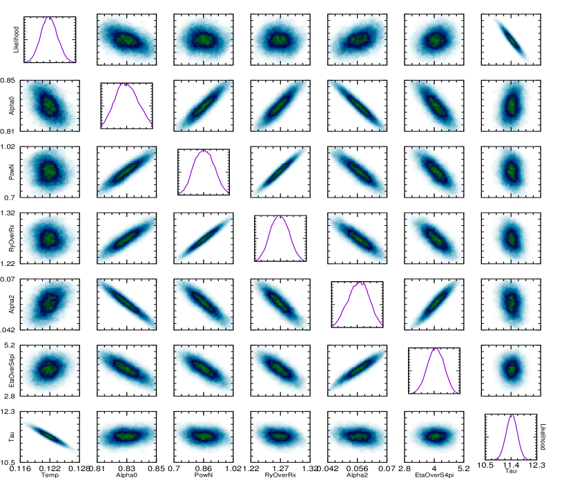
Figure 1: Likelihood analysis for ALICE data in the 30-40 $\%$ centrality bin provided by the MADAI package. The horizontal and vertical axes show the chosen prior ranges for the parameters $\mathcal{P}$. From left to right (bottom to top): $T$ (MeV), $\alpha_{0}$, $n$, $R_{y}/R_{x}$, $\alpha_{2}$, $\eta/s$, $\tau$ (fm/$c$). Plots on the diagonal show posterior likelihood distributions. The off-diagonal plots show correlations between parameters.

IV Fit Results and Uncertainty Analysis

With the preparations from the previous sections in place we go ahead and analyze the available data for each energy and centrality bin. The fit results are generally of good quality despite the relatively large RFR fit range. As an example we discuss here the 30-40% centrality bin for ALICE data in detail. Fig. 1 shows the results for the fit parameter set $\mathcal{P}$ from the statistical analysis for fits in the RFR of this data set. The likelihood plots on the diagonal of Fig. 1 show well defined peaks. The off-diagonal plots show correlations between fit parameters. The preferred (average) values for this ALICE centrality bin are $\tau=11.41$ fm/$c$, $T$=121.9 MeV, $\alpha_{0}$=0.830$c$, $n$=0.87, $R_{y}/R_{x}$=1.270, $\alpha_{2}$=0.0564$c$, $\eta/s$=4.06/4$\pi$. Recall that the values for the external parameters $c_{\tau}$ and $c_{s}^{2}$ as well as for the chemical potentials, and the regular fit range used are given in Tab. 1 and 2, respectively.

Although we have already eliminated some parameters from the blastwave there are still correlations between the remaining parameters in $\mathcal{P}$. Most prominently there is an expected anti-correlation between freeze-out time and temperature which comes from the constraint on the overall number of particles. Surprisingly there is no pronounced anti-correlation between temperature and radial flow parameter $\alpha_{0}$, which means that the choice of three different hadrons to fit, and the sizes of the fit ranges, are sufficient to cleanly separate thermal and collective motion. We note a correlation between the elliptic flow parameter $\alpha_{2}$ and $\eta/s$. As expected, for larger values of $P_{T}$ these two parameters move the elliptic flow in different directions, i.e. an increase in one of these parameters will necessitate an increase in the other one. The correlations seen in this centrality bin are found to be qualitatively true for the other energies and centrality bins as well.

Using the preferred parameters, we calculate the transverse momentum spectra and elliptic flow $v_{2}$ for the 30-40% ALICE centrality bin. We show these calculations together with the data in Fig. 2. The bottom of the figure shows the ratio of calculation over data. For the majority of $P_{T}$-bins the deviation is less than 5%, and it rarely exceeds 20%. If the experimental error bars are included, the ratio is consistent with one almost everywhere in the RFR.

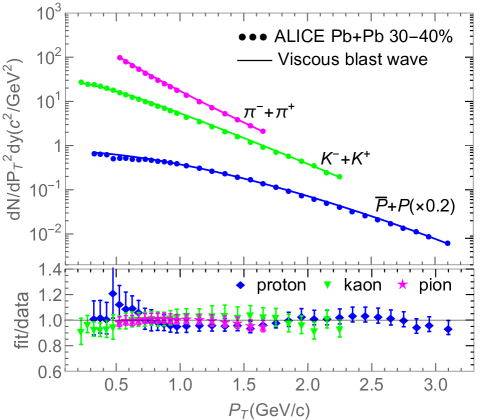
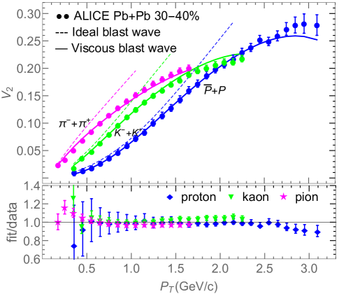
Figure 2: Left panel: Transverse momentum spectra for pions, kaons and protons (solid lines), respectively, using the extracted, preferred fit parameters for the ALICE 30-40 $\%$ centrality bin. We also show the ALICE data used for the fit (circles) with statistical and systematic errors summed in quadrature. Right panel: Elliptic flow $v_{2}$ for pions, kaons and protons (solid lines) for the same parameters, together with ALICE data (circles). We also show the elliptic flow calculated in the ideal case, i.e. without the shear stress term $\delta f$ in the particle distribution (dashed lines). Ratios of calculations to dtata are shown below the panels.

Centrality	$\tau$ (fm/$c$)	$T$ (MeV)	$\alpha_{0}/c$	$n$	$R_{y}/R_{x}$	$\alpha_{2}/c$	$4\pi\eta/s$
ALICE 2.76 TeV
10-20%	14.76	113.3	0.856	0.78	1.143	0.0355	5.89
20-30%	13.05	118.0	0.839	0.80	1.200	0.0517	5.45
30-40%	11.41	121.9	0.830	0.87	1.270	0.0564	4.06
40-50%	9.96	125.5	0.835	1.07	1.362	0.0472	2.46
50-60%	8.72	130.1	0.823	1.27	1.433	0.0427	1.66
PHENIX 0.2 TeV
10-20%	10.9	121.2	0.734	0.80	1.090	0.0463	3.32
20-30%	9.28	123.5	0.742	0.94	1.167	0.0528	1.98
30-40%	9.08	124.2	0.733	0.90	1.227	0.0576	1.64
40-50%	7.15	132.2	0.704	1.03	1.312	0.0631	1.08
50-60%	6.96	135.3	0.689	1.00	1.354	0.0630	0.93
MUSIC 0.2 TeV
$b=7.5$ fm	8.0	131.9	0.768	0.9	1.220	0.0357	1.06

Table 4: Preferred values for the parameter set $\mathcal{P}$ obtained for different centrality bins for ALICE and PHENIX data in the regular fit range. We also show the results of fits to MUSIC pseudo data as discussed in the text.

We analyze other centrality bins of ALICE analogously. The results for all ALICE centrality bins are summarized in Tab. 4. We note that the general trends of parameters as functions of centrality are consistent with expectations. The freeze-out temperature $T_{\mathrm{fo}}$ rises toward smaller systems. The boundary velocity $\alpha_{0}$ reduces slightly at the same time. The (spatially) averaged radial velocity (not shown) drops more significantly due to the concurrent change in the radial shape parameter $n$. These systematic trends give an important qualitative check of the fit results. However, we will not be interested in further interpretation of fit parameters other than the temperature and specific shear viscosity. The ALICE data sets provide us with a range of temperatures from roughly 113 MeV to 130 MeV.

Generally, the azimuthal flow deformation parameter $\alpha_{2}$ and spatial deformation $R_{y}/R_{x}$ as well as the specific shear viscosity $\eta/s$ are most sensitive to the elliptic flow data. We indicate the sensitivity of the calculated elliptic flow on $\eta/s$ at freeze-out by also showing in Fig. 2 the elliptic flow computed with the same parameters but without the correction term $\delta f$. As expected, at large $P_{T}$ the corrections from $\delta f$ are largest, thus extracted values of $\eta/s$ are very sensitive to $v_{2}$ at large $P_{T}$. Note however that despite the $p^{2}$-dependence of $\delta f$ in the local rest frame, the correction to $v_{2}$ due to $\delta f$ does not have to strictly vanish at small transverse momenta $P_{T}$ in the lab frame. We have to be mindful that $\delta f$ can not be too large. As discussed earlier, higher order corrections in shear stress would have to be taken into account if $\delta f\approx f$. We have chosen the RFR such that $v_{2}$ starts to deviate from the equilibrium behavior at large $P_{T}$, but we generally exclude points for which the slope of $v_{2}$ turns negative. In the RFR we find that the viscous correction is largest for protons, topping out at 19% for the largest $P_{T}$-bin in the spectrum for the 40-50% centrality bin. For kaons and pions the largest corrections for the spectra we find are 11% and 4%, respectively. The typical size of viscous corrections is much smaller than the maximum numbers quoted here.

We repeat the analysis with data from PHENIX in 200 GeV Au+Au collisions. The preferred, average values are also summarized in Tab. 4. The fits with preferred parameter values for one centrality bin are shown in Fig. 3 together with PHENIX data. The behavior of parameters as a function of centrality is similar to the one discussed for the ALICE data sets. The extracted temperatues range, roughly 122 MeV to 136 MeV overlaps with ALICE. It is an important consistency check that the extracted values for $\eta/s$ are consistent between ALICE data taken at $\sqrt{s_{NN}}=2.76$ TeV and PHENIX data taken at $\sqrt{s_{NN}}=0.2$ TeV, within uncertainties. We summarize the results for $\eta/s$ vs temperature $T$ from all data sets in Fig. 4. The main qualitative feature is a decrease in $\eta/s$ with increasing temperature, as would be expected from general principles. However, values close to the lower bound are already reached at the upper end of the temperature range.

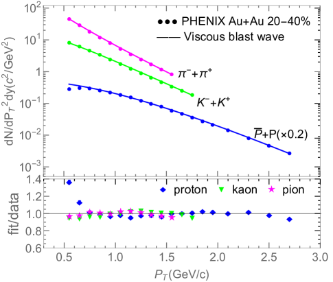
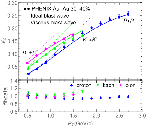
Figure 3: Same as Fig. 2 for the PHENIX 30-40 $\%$ centrality bin (20-40% for the spectrum). Statistical errors only are shown for PHENIX spectra.

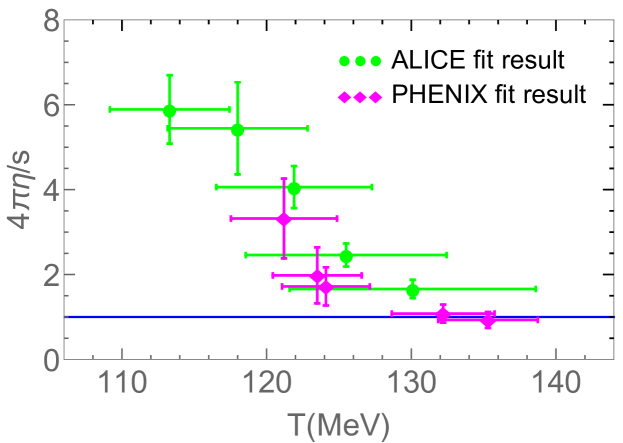
Figure 4: Specific shear viscosity $\eta/s$ at corresponding kinetic freeze-out temperature $T$ extracted from the available ALICE and PHENIX centrality bins. Uncertainties shown are combined uncertainties of type (III) and (IV) explained in the text. Note that the values of the chemical potentials for stable hadrons are non-zero for all of these points.

Let us now turn to a discussion of the uncertainties in our analysis. We can group them into four categories, ranging from basic statistical errors to rather fundamental in nature: (I) Fundamental limitations in our freeze-out ansatz that are shared between blastwave and fluid dynamics, e.g. from the validity of the Navier-Stokes approximation, and the assumption of a sharp freeze-out hypersurface. (II) Uncertainties and biases from assumptions made specifically in our blastwave model, e.g. the simple ansatz for the freeze-out hypersurface and the flow field, and the lack of resonance decays and bulk stress effects. (III) Uncertainties from our choice of external parameters and choice of fit ranges. (IV) Uncertainties from the errors in experimental data and the quality of the Gaussian emulator. A thorough analysis of item (I) is beyond the scope of this paper and can not be achieved within the blastwave model. However we will attempt to analyze the other three sources of uncertainty.

Fit range (GeV/c)	proton	kaon	pion	$T$ (MeV)	$4\pi\eta/s$
Low (LFR)	0.325-2.05	0.225-1.25	0.19-0.825	113.4	3.85
Regular (RFR)	0.325-3.1	0.225-2.25	0.525-1.65	121.9	4.06
High (HFR)	1.25-3.1	0.725-2.25	0.825-1.65	125.2	3.43

Table 5: Definitions of different fit ranges for ALICE spectrum data in the 30-40 $\%$ centrality bin. The ranges for $v_{2}$ data are chosen commensurately. Also shown are the extracted temperature and specific shear viscosity for each fit range.

Uncertainties in extracted parameters from the error bars in our data sets and statistical analysis (type IV), are provided by the MADAI code. We quote the widths $\sigma_{T}^{\mathrm{stat}}$, $\sigma_{\eta}^{\mathrm{stat}}$ of temperature and specific shear viscosity for each centraliy bin and energy. We estimate uncertainties summarized under (III) by systematically varying the underlying assumptions. E.g., as discussed earlier we choose alternative fit ranges which are shifted to lower (LFR) or larger (HFR) $P_{T}$. Limitations apply as we do not want to push too far into regions where we expect our blastwave to fail, see the discussion of fit ranges in Sec. III. We discuss results once more for the 30-40 $\%$ ALICE centrality bin as an example. For the uncertainty analysis we focus on the results for the extracted temperature and specific shear viscosity. Table 5 shows the three fit ranges, LFR, RFR, HFR for all three particle species for this data set. Both temperature and $\eta/s$ show moderate dependencies on the fit range. This is expected for the temperature, where a change in $P_{T}$ samples different admixtures of resonance decays in spectra with different slopes and thus apparent temperatures. We parameterize the deviations seen from the RFR values as Gaussian fluctuations with widths $\sigma_{k}^{\mathrm{range}}$ ($k=T,\eta$). We repeat this analysis for all other centralities and energies with qualitatively similar results.

	$\mu_{\pi}$ (MeV)	T (MeV)	$4\pi\eta/s$
less	46	121.0	4.01
regular	61	121.9	4.06
more	76	122.7	3.85

Table 6: The freeze-out temperature $T$ and specific shear viscosity $\eta/s$ extracted for different values of pion chemical potential $\mu_{\pi}$ as explained in the text, for the ALICE 30-40$\%$ centrality bin.

	$c_{s}^{2}(c^{2})$	$T$ (MeV)	$4\pi\eta/s$
small	0.15	121.8	4.27
regular	0.166	121.9	4.06
large	0.182	122.0	3.85

Table 7: The same as Tab. 6 for a variation of the speed of sound squared $c_{s}^{2}$ for the ALICE 30-40$\%$ centrality bin.

	$c_{\tau}$	$T$ (MeV)	$4\pi\eta/s$
small	0.666	121.6	3.82
regular	0.720	121.9	4.06
large	0.781	121.2	4.12

Table 8: The same as Tab. 6 for a variation of time-averaged surface velocity parameter $c_{\tau}$ for the ALICE 30-40$\%$ centrality bin.

Origin of uncertainty	Stat. analysis	fit range	$\mu_{\pi}$	$c_{s}^{2}$	$c_{\tau}$	total $\sigma$
$T$ (MeV)	1.90	4.97	0.69	0.08	0.29	5.38
$4\pi\eta/s$	0.35	0.26	0.10	0.17	0.13	0.50

Table 9: A summary of uncertainties $\sigma_{T}^{i}$ and $\sigma_{\eta}^{i}$ for temperature and specific shear viscosity, respectively, for the 30-40% ALICE centrality bin. Here $i$ refers to the different contributions discussed in the text.

As discussed earlier we also study the effects of variations in the chemical potential, speed of sound squared, and the expansion parameter $c_{\tau}$. Table 6 shows the values for $T$ and $\eta/s$ extracted for the 30-40% ALICE centrality bin for $\pm 15$ MeV variations in the pion chemical potential. We find that the temperature is rather insensitive to variations of $\mu_{\pi}$ while $\eta/s$ displays moderate sensitivity. We again assign Gaussian widths $\sigma_{k}^{\mu}$ ($k=T,\eta$) for the uncertainty from this source. We proceed similarly with variations in $c_{s}^{2}$, see Tab. 7 and $c_{\tau}$ (Tab. 8). In both cases we find again very little influence on the extracted temperature. Finally we combine the uncertainties of types (III) and (IV) by adding the individual widths $\sigma^{i}_{T}$ and $\sigma^{i}_{\eta}$ in quadrature. Note that this assumption of Gaussian behavior here is simply an approximation. The error bars in $T$ and $\eta/s$ shown in Fig. 4 are the result of this analysis. Table 9 summarizes the uncertainties for the ALICE 30-40% centrality bin.

Finally we make an attempt to quantify uncertainties of type (II). To this end we use particle spectra and $v_{2}$ created with the viscous fluid dynamic code MUSIC Ryu:2015vwa , and apply the same analysis that we have used for ALICE and PHENIX data. In this case we know the precise temperature of freeze-out (set to 135 MeV) and the specific shear viscosity (set to $\eta/s=1/4\pi$ at freeze-out and throughout the evolution), and we can compare to the result of our analysis. We use an average (i.e. smooth) Au+Au collision system with impact parameter $b=7.5$ fm. The key difference between the fluid dynamic system at freeze-out and the blastwave are the more realistic freeze-out hypersurface, more complex shape of the flow field, and the presence of both bulk stress at freeze-out and hadronic decays after freeze-out in MUSIC. By comparing our extracted temperature and specific shear viscosity with the one set in the fluid dynamic system we can gain insights what deviations we have to expect through the absence of these features in the blastwave.

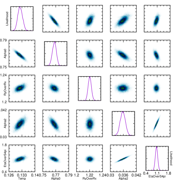
Figure 5: Likelihood and correlations for the parameter set $\mathcal{P}$, reduced by $n$, for a fit to MUSIC pseudo data.

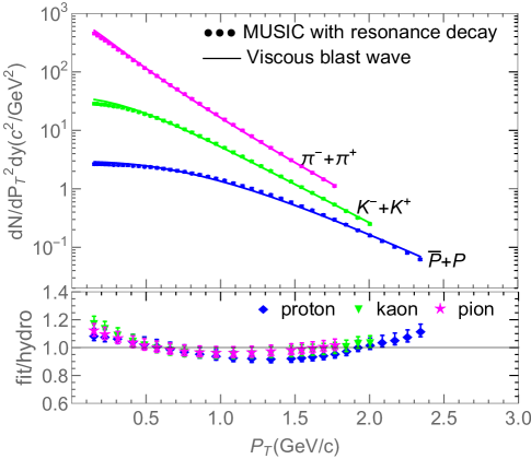
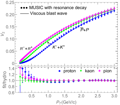
Figure 6: Same as Fig. 2 but for a fit to spectra and elliptic flow generated by the MUSIC code as described in the text.

We need to specify a fit range and error bars for the MUSIC pseudo data. We choose them to be roughly consistent with the fit ranges used in the actual data analysis. These values can be found in Tables 1 and 3. The relative error of 2% mentioned for $v_{2}$ in the latter table is supplemented by a pedestal of 0.001 which needs to be added to give data points very close to zero reasonably sized errors. In our analysis we find that the MUSIC pseudo data leads to a larger degree of degeneracy coming from correlations between fit parameters. We have made the choice to remove the parameter $n$ from the fit parameter tuple $\mathcal{P}$ and to set its value to $n=0.9$, commensurate with values found from RHIC data for similar impact parameter. This reduction leads to crisply defined fits for the remaining parameters. We show the likelihood and correlation plot for the MUSIC analysis in Fig. 5, and the preferred values extracted at the bottom of Tab. 4. We find $T=131.9$ MeV and $\eta/s=1.06$. Fig. 6 shows calculations with our blastwave using the extracted parameters together with the MUSIC pseudo data and assigned error bars.

$n$ was chosen to be removed from the fit as a somewhat obscure parameter that we have no further interest in. In fact such a shape parameter for the flow field is absent in many simpler blastwave parameterizations on the market. Nevertheless one might worry what this choice means for our uncertainty analysis. The same can be said about our choice or error bars for the pseudo data. We have varied both $n$ and the error bars of the MUSIC pseudo data. We find that the extracted value of the temperature is rather stable, at about $3$ MeV below the value set in MUSIC. The extracted value for the specific shear viscosity can change by up to 30%, for reasonable variations of $n$. In conclusion, our exploration of uncertainties of type (II) for this data set suggest that temperatures extracted with the blastwave are likely biased to find lower than actual temperatures, but this bias is only about 3 MeV. There is also an additional uncertainly on $\eta/s$ of up to 30% which could be added to the total tally of uncertainties. Note again that Fig. 4 only shows the uncertainty in $T$ and $\eta/s$ from type (III) and (IV). Our analysis of type (II) uncertainties could certainly be made more quantitative. In principle we have to run the same analysis described here for every ($T$-$\eta/s$) point that we have extracted from data. We keep this discussion for a future publication.

V Discussion

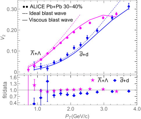
Figure 7: Left panel: Transverse momentum spectra for $\Lambda$s and deuterons (solid lines), respectively, calculated for the 20-40 $\%$ centrality bin in Pb+Pb collisions together with ALICE data (symbols). Right panel: Elliptic flow $v_{2}$ for $\Lambda+\bar{\Lambda}$ and $d+\bar{d}$ (solid lines) in the 30-40% centrality bin together with ALICE data (circles). We agin show the elliptic flow calculated in the ideal case as well. In both cases the preferred parameters for the 30-40% centrality bin extracted for stable charged hadrons has been used.

We have introduced a blastwave model with viscous corrections due to shear stress in the Navier-Stokes approximation. The blastwave model can obtain excellent fits to hadron spectra and $v_{2}$ over a large range of $P_{T}$. The viscous correction term helps to describe the slow down of the growth of $v_{2}$ with $P_{T}$. This model provides a reliable instrument that can give useful snapshots of the dynamically evolving fireball.

To further demonstrate the usefulness we plot predictions for the spectra and $v_{2}$ for two more particles, the $\Lambda$ baryon and the deuteron $d$, in a mid-central bin as examples. The results are shown in Fig. 7 together with ALICE data Acharya:2017dmc ; ABELEV:2013zaa ; Abelev:2014pua . Note that our calculation is a prediction in the sense that $\Lambda$ and deuteron data have not been used to fix the blastwave parameters. Chemical potentials for both species have been fixed to 344 and 314 MeV respectively. We find overall good agreement for this centrality bin. This is interesting since there have been questions in both cases about the validity of a common freeze-out with stable hadrons. In particular the deuteron is often thought to be emerging from coalescence processes after freeze-out Acharya:2017dmc ; Adamczyk:2016gfs ; Zhu:2017zlb . We find that, whatever the detailed mechnism of deuteron creation, the spectra and elliptic flow are described reasonably well by the same temperature and flow field that also describes stable hadrons, at least in mid-central collisions.

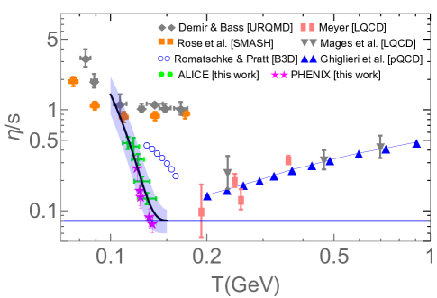
Figure 8: The results of this paper compared to various calculations of the specific shear viscosity $\eta/s$ as a function of temperature. A line and uncertainty band have been drawn through our points to guide the eye. Details in the text.

Let us now turn to a discussion of the particular application of our blastwave we have focused on here. From two different collision systems, Pb+Pb at LHC energy and Au+Au at top RHIC energy we have extracted several $\eta/s$-vs-$T$ points that are consistent with each other within estimated uncertainties. They give us a band, indicated in the figure, that roughly stretches from 110 MeV to 140 MeV. The center line of the band can be approximately parameterized as $\eta/s=1.47\times 10^{5}\times(0.155-T)^{4}+0.08$ where $T$ is measured in GeV. Note again that uncertainties of type (II) are not included here. The bias discussed at the end of the last section indicates that points might have to be shifted up in temperature by about 3 MeV. We also show results for the hadronic phase from hadronic cascades URQMD Demir:2008tr , B3D Romatschke:2014gna and SMASH Rose:2017bjz . They generally show larger values of $\eta/s$ above $T\sim 100$ MeV. One could speculate that below $T\sim 100$ MeV the results might converge within uncertainties, as the URQMD and SMASH results switch their behavior to a temperature slope similar to our results. Unfortunately we do not have the data points to confirm this. We also show several calculations of the specific shear viscosity in the QGP phase, from lattice QCD Meyer:2007ic ; Meyer:2009jp ; Mages:2015rea and using next-to-leading perturbative QCD Ghiglieri:2018dib . Overall these results together are consistent with the idea of a minimum of the specific shear viscosity around the pseudocritical temperature $T_{c}$. Our result specifically would indicate a rather broad minimum where interactions in the hadronic phase continue to be strong just below $T_{c}$ while hadronic transport suggests a more abrupt change below $T_{c}$.

However, we need to keep in mind that relatively large chemical potentials for stable hadrons build up in the collision systems that we have analyzed here. E.g. the chemical potential for pions is as large as 70 MeV at the lowest temperature points we have extracted. Thus Fig. 8 is a projection of a more complicated plot with additional chemical potential axes. Studies with hadronic transport have indicated that finite chemical potentials can indeed lead to smaller values of $\eta/s$ Demir:2008tr in this picture.

The fate of $\eta/s$ in the hadronic phase continues to be intriguing. We have added a scenario, based on extraction from data, that predicts a steep rise of $\eta/s$ while the temperature drops from 140 and 110 MeV and chemical potentials increase. Our approach is rooted in data taken in heavy ion collisions but has built in uncertainties. We have quantified the more accessible uncertainties (IV) and (III) related to the analysis itself and to systemic uncertainties from choices made during the analysis. We have also made a first attempt to estimate the weaknesses of the blastwave compared to a full fluid dynamic simulation, i.e. uncertainties of type (II). More fundamental uncertainties remain which may be quantified elsewhere. Certain aspects of the current analysis will be improved in the near term future. For example the detailed energy dependence of the shear stress term, parameterized by $\lambda$, and the effects of bulk stress could be included, albeit at the expense of adding two parameters to the analysis. One could also include an analysis of the asymmetry coefficient $v_{4}$, which requires a generalization of both hypersurface and flow field of the blastwave. Lastly, resonances and their decays could in principle be included in the calculation.

- (1) J. C. Collins and M. J. Perry, “Superdense Matter: Neutrons Or Asymptotically Free Quarks?”, Phys. Rev. Lett. 34, 1353 (1975).
- (2) E. V. Shuryak, “Quark-Gluon Plasma and Hadronic Production of Leptons, Photons and Psions”, Phys. Lett. 78B, 150 (1978).
- (3) M. Gyulassy and L. McLerran, “New forms of QCD matter discovered at RHIC”, Nucl. Phys. A 750, 30 (2005).
- (4) E. Shuryak, “Physics of Strongly coupled Quark-Gluon Plasma”, Prog. Part. Nucl. Phys. 62, 48 (2009).
- (5) P. F. Kolb, P. Huovinen, U. W. Heinz and H. Heiselberg, “Elliptic flow at SPS and RHIC: From kinetic transport to hydrodynamics”, Phys. Lett. B 500, 232 (2001).
- (6) P. Huovinen, P. F. Kolb, U. W. Heinz, P. V. Ruuskanen and S. A. Voloshin, “Radial and elliptic flow at RHIC: Further predictions”, Phys. Lett. B 503, 58 (2001).
- (7) P. Romatschke and U. Romatschke, “Viscosity Information from Relativistic Nuclear Collisions: How Perfect is the Fluid Observed at RHIC?”, Phys. Rev. Lett. 99, 172301 (2007).
- (8) K. Dusling and D. Teaney, “Simulating elliptic flow with viscous hydrodynamics”, Phys. Rev. C 77, 034905 (2008).
- (9) B. Schenke, S. Jeon and C. Gale, “Anisotropic flow in TeV Pb+Pb collisions at the LHC”, Phys. Lett. B 702, 59 (2011).
- (10) U. Heinz and R. Snellings, “Collective flow and viscosity in relativistic heavy-ion collisions”, Ann. Rev. Nucl. Part. Sci. 63, 123 (2013).
- (11) P. Kovtun, D. T. Son and A. O. Starinets, “Viscosity in strongly interacting quantum field theories from black hole physics”, Phys. Rev. Lett. 94, 111601 (2005).
- (12) D. Teaney, “The Effects of viscosity on spectra, elliptic flow, and HBT radii”, Phys. Rev. C 68, 034913 (2003).
- (13) H. Song, S. A. Bass and U. Heinz, “Viscous QCD matter in a hybrid hydrodynamic+Boltzmann approach”, Phys. Rev. C 83, 024912 (2011).
- (14) H. Song, S. A. Bass, U. Heinz, T. Hirano and C. Shen, “Hadron spectra and elliptic flow for 200 A GeV Au+Au collisions from viscous hydrodynamics coupled to a Boltzmann cascade”, Phys. Rev. C 83, 054910 (2011) Erratum: [Phys. Rev. C 86, 059903 (2012)].
- (15) M. Prakash, M. Prakash, R. Venugopalan and G. Welke, “Nonequilibrium properties of hadronic mixtures”, Phys. Rept. 227, 321 (1993).
- (16) S. Muroya and N. Sasaki, “A Calculation of the viscosity over entropy ratio of a hadronic gas”, Prog. Theor. Phys. 113, 457 (2005).
- (17) A. Dobado and F. J. Llanes-Estrada, “The Viscosity of meson matter”, Phys. Rev. D 69, 116004 (2004).
- (18) J. W. Chen and E. Nakano, “Shear viscosity to entropy density ratio of QCD below the deconfinement temperature”, Phys. Lett. B 647, 371 (2007).
- (19) K. Itakura, O. Morimatsu and H. Otomo, “Shear viscosity of a hadronic gas mixture”, Phys. Rev. D 77, 014014 (2008).
- (20) A. Dobado, F. J. Llanes-Estrada and J. M. Torres-Rincon, “eta/s and phase transitions”, Phys. Rev. D 79, 014002 (2009).
- (21) N. Demir and S. A. Bass, “Shear-Viscosity to Entropy-Density Ratio of a Relativistic Hadron Gas”, Phys. Rev. Lett. 102, 172302 (2009).
- (22) D. Fernandez-Fraile and A. Gomez Nicola, “Transport coefficients and resonances for a meson gas in Chiral Perturbation Theory”, Eur. Phys. J. C 62, 37 (2009).
- (23) P. Romatschke and S. Pratt, “Extracting the shear viscosity of a high temperature hadron gas”, arXiv:1409.0010 [nucl-th].
- (24) J.-B. Rose, J. M. Torres-Rincon, A. Schäfer, D. R. Oliinychenko and H. Petersen, “Shear viscosity of a hadron gas and influence of resonance lifetimes on relaxation time”, arXiv:1709.03826 [nucl-th].
- (25) H. Niemi, G. S. Denicol, P. Huovinen, E. Molnar and D. H. Rischke, “Influence of a temperature-dependent shear viscosity on the azimuthal asymmetries of transverse momentum spectra in ultrarelativistic heavy-ion collisions”, Phys. Rev. C 86, 014909 (2012).
- (26) J. E. Bernhard, P. W. Marcy, C. E. Coleman-Smith, S. Huzurbazar, R. L. Wolpert and S. A. Bass, “Quantifying properties of hot and dense QCD matter through systematic model-to-data comparison”, Phys. Rev. C 91, no. 5, 054910 (2015).
- (27) C. Gale, S. Jeon and B. Schenke, “Hydrodynamic Modeling of Heavy-Ion Collisions”, Int. J. Mod. Phys. A 28, 1340011 (2013).
- (28) P. Romatschke and U. Romatschke, “Relativistic Fluid Dynamics In and Out of Equilibrium – Ten Years of Progress in Theory and Numerical Simulations of Nuclear Collisions”, arXiv:1712.05815 [nucl-th].
- (29) H. B. Meyer, “A Calculation of the shear viscosity in SU(3) gluodynamics”, Phys. Rev. D 76, 101701 (2007).
- (30) H. B. Meyer, “Transport properties of the quark-gluon plasma from lattice QCD”, Nucl. Phys. A 830, 641C (2009).
- (31) S. W. Mages, S. Borsányi, Z. Fodor, A. Schäfer and K. Szabó, “Shear Viscosity from Lattice QCD”, PoS LATTICE 2014, 232 (2015).
- (32) M. Haas, L. Fister and J. M. Pawlowski, “Gluon spectral functions and transport coefficients in Yang–Mills theory”, Phys. Rev. D 90, 091501 (2014).
- (33) N. Astrakhantsev, V. Braguta and A. Kotov, “Temperature dependence of shear viscosity of –gluodynamics within lattice simulation”, JHEP 1704, 101 (2017).
- (34) P. B. Arnold, G. D. Moore and L. G. Yaffe, “Transport coefficients in high temperature gauge theories. 1. Leading log results”, JHEP 0011, 001 (2000).
- (35) P. B. Arnold, G. D. Moore and L. G. Yaffe, “Transport coefficients in high temperature gauge theories. 2. Beyond leading log”, JHEP 0305, 051 (2003).
- (36) J. Ghiglieri, G. D. Moore and D. Teaney, “QCD Shear Viscosity at (almost) NLO”, JHEP 1803, 179 (2018).
- (37) L. P. Csernai, J. I. Kapusta and L. D. McLerran, “On the Strongly-Interacting Low-Viscosity Matter Created in Relativistic Nuclear Collisions”, Phys. Rev. Lett. 97, 152303 (2006).
- (38) G. D. Westfall, J. Gosset, P. J. Johansen, A. M. Poskanzer, W. G. Meyer, H. H. Gutbrod, A. Sandoval and R. Stock, “Nuclear Fireball Model for Proton Inclusive Spectra from Relativistic Heavy Ion Collisions”, Phys. Rev. Lett. 37, 1202 (1976).
- (39) E. Schnedermann, J. Sollfrank and U. W. Heinz, “Thermal phenomenology of hadrons from 200-A/GeV S+S collisions”, Phys. Rev. C 48, 2462 (1993).
- (40) F. Retiere and M. A. Lisa, “Observable implications of geometrical and dynamical aspects of freeze out in heavy ion collisions”, Phys. Rev. C 70, 044907 (2004).
- (41) A. Jaiswal and V. Koch, “A viscous blast-wave model for relativistic heavy-ion collisions”, arXiv:1508.05878 [nucl-th].
- (42) M. Damodaran, D. Molnar, G. G. Barnaföldi, D. Berényi and M. Ferenc Nagy-Egri, “Testing and improving shear viscous phase space correction models”, arXiv:1707.00793 [nucl-th].
- (43) F. Cooper and G. Frye, “Comment on the Single Particle Distribution in the Hydrodynamic and Statistical Thermodynamic Models of Multiparticle Production”, Phys. Rev. D 10, 186 (1974).
- (44) B. Schenke, S. Jeon and C. Gale, “(3+1)D hydrodynamic simulation of relativistic heavy-ion collisions”, Phys. Rev. C 82, 014903 (2010).
- (45) S. Ryu, J.-F. Paquet, C. Shen, G. S. Denicol, B. Schenke, S. Jeon and C. Gale, “Importance of the Bulk Viscosity of QCD in Ultrarelativistic Heavy-Ion Collisions”, Phys. Rev. Lett. 115, no. 13, 132301 (2015).
- (46) J. Adam et al. [ALICE Collaboration], “Centrality dependence of the nuclear modification factor of charged pions, kaons, and protons in Pb-Pb collisions at TeV”, Phys. Rev. C 93, no. 3, 034913 (2016).
- (47) B. B. Abelev et al. [ALICE Collaboration], “Elliptic flow of identified hadrons in Pb-Pb collisions at TeV”, JHEP 1506, 190 (2015).
- (48) A. Adare et al. [PHENIX Collaboration], “Spectra and ratios of identified particles in Au+Au and +Au collisions at GeV”, Phys. Rev. C 88, no. 2, 024906 (2013).
- (49) A. Adare et al. [PHENIX Collaboration], “Measurement of the higher-order anisotropic flow coefficients for identified hadrons in AuAu collisions at = 200 GeV”, Phys. Rev. C 93, no. 5, 051902 (2016).
- (50) J. Sollfrank, P. Koch and U. W. Heinz, “Is there a low p(T) ’anomaly’ in the pion momentum spectra from relativistic nuclear collisions?”, Z. Phys. C 52, 593 (1991).
- (51) B. Abelev et al. [ALICE Collaboration], “Centrality dependence of , K, p production in Pb-Pb collisions at = 2.76 TeV”, Phys. Rev. C 88, 044910 (2013).
- (52) MADAI collaboration, https://madai-public.cs.unc.edu/, accessed June 20, 2016.
- (53) J. E. Bernhard, J. S. Moreland, S. A. Bass, J. Liu and U. Heinz, “Applying Bayesian parameter estimation to relativistic heavy-ion collisions”, Phys. Rev. C 94, 024907 (2016).
- (54) H. Song and U. W. Heinz, “Interplay of shear and bulk viscosity in generating flow in heavy-ion collisions”, Phys. Rev. C 81, 024905 (2010).
- (55) S. S. Adler et al. [PHENIX Collaboration], “Suppressed pi0̂ production at large transverse momentum in central Au+Au collisions at S(NN)**1/2 = 200 GeV”, Phys. Rev. Lett. 91, 072301 (2003).
- (56) D. Teaney, “Chemical freezeout in heavy ion collisions”, preprint arxiv:nucl-th/0204023.
- (57) Pasi Huovinen and Peter Petreczky “QCD Equation of State and Hadron Resonance Gas”, Nucl. Phys. A837:26-53 (2010).
- (58) T. Hirano and K. Tsuda, “The Effect of early chemical freezeout on radial and elliptic flow from a full 3-D hydrodynamic model”, preprint arxiv:nucl-th/0202033.
- (59) S. Acharya et al. [ALICE Collaboration], “Measurement of deuteron spectra and elliptic flow in Pb–Pb collisions at = 2.76 TeV at the LHC”, Eur. Phys. J. C 77, no. 10, 658 (2017).
- (60) B. B. Abelev et al. [ALICE Collaboration], “Multi-strange baryon production at mid-rapidity in Pb-Pb collisions at = 2.76 TeV”, Phys. Lett. B 728, 216 (2014) Erratum: [Phys. Lett. B 734, 409 (2014)].
- (61) B. B. Abelev et al. [ALICE Collaboration], “Elliptic flow of identified hadrons in Pb-Pb collisions at TeV”, JHEP 1506, 190 (2015).
- (62) L. Adamczyk et al. [STAR Collaboration], “Measurement of elliptic flow of light nuclei at 200, 62.4, 39, 27, 19.6, 11.5, and 7.7 GeV at the BNL Relativistic Heavy Ion Collider”, Phys. Rev. C 94, no. 3, 034908 (2016).
- (63) L. Zhu, H. Zheng, C. M. Ko and Y. Sun, “Light nuclei production in Pb+Pb collisions at TeV”, preprint arXiv:1710.05139 [nucl-th].