Necklaces count polynomial parametric osculants

Abstract.

We consider the problem of geometrically approximating a complex analytic curve in the plane by the image of a polynomial parametrization $t\mapsto(x_{1}(t),x_{2}(t))$ of bidegree $(d_{1},d_{2})$. We show the number of such curves is the number of primitive necklaces on $d_{1}$ white beads and $d_{2}$ black beads. We show that this number is odd when $d_{1}=d_{2}$ is squarefree and use this to give a partial solution to a conjecture by Rababah. Our results naturally extend to a generalization regarding hypersurfaces in higher dimensions. There, the number of parametrized curves of multidegree $(d_{1},\ldots,d_{n})$ which optimally osculate a given hypersurface are counted by the number of primitive necklaces with $d_{i}$ beads of color $i$.

1. Introduction

Given a generic complex analytic curve $\mathcal{C}\subset\mathbb{C}^{2}$ through the origin defined locally by the graph of $g(x_{1})=\sum_{i=1}^{\infty}c_{i}x_{1}^{i}$ it is a common task to approximate $\mathcal{C}$ at the origin by a member of a simpler family of curves. The family we consider are curves which arise as the image of some polynomial map

$${\bf x}(t):\mathbb{C}\to\mathbb{C}^{2}$$

$$t\mapsto(x_{1}(t),x_{2}(t))$$

of bidegree $\textbf{d}:=(d_{1},d_{2})$ and the notion of approximation we use is the degree of vanishing of the univariate power series $f(x_{1},x_{2})=x_{2}(t)-g(x_{1}(t))$ at $t=0$. We call ${\bf x}(t)$ a $k$-fold d-parametrization when it is generically $k$-to-one. Up to reparametrization, there are finitely many $k$-fold d-parametrizations which meet $\mathcal{C}$ to the expected maximal approximation order $d_{1}+d_{2}$ (Corollary 3.7). Images of such parametrizations are curves of bidegree $\frac{\textbf{d}}{k}:=\left(\frac{d_{1}}{k},\frac{d_{2}}{k}\right)$ and are called $\frac{\textbf{d}}{k}$-interpolants. Because $d_{1}+d_{2}$ is the maximal approximation order attainable by a $(d_{1},d_{2})$-parametrization, we may assume that $f(x_{1},x_{2})$ is a polynomial in $\mathbb{C}[x_{1},x_{2}]$ by truncating higher order terms. We show that the number of d-interpolants of a generic curve is the number of primitive necklaces on $d_{1}$ white beads and $d_{2}$ black beads (Corollary 1.2).

When $f\in\mathbb{R}[x_{1},x_{2}]$, and $d_{1}=d_{2}$, Rababah conjectured that there exists at least one real d-interpolant [11]. A similar conjecture was made by Höllig and Koch which includes the case when interpolation points are distinct and also conjectures that local approximation of a curve at a point occurs as the limit of the interpolation of distinct points on that curve [7]. The cubic case was resolved and analyzed thoroughly by DeBoor, Sabin, and Höllig [2]. Scherer showed that there are eight $(4,4)$-interpolants and investigated bounds on the number of those which are real [12]. For a family of curves known as “circle-like curves”, Rababah’s conjecture has been resolved for all $d_{1}=d_{2}$ [9] as well as for generic curves up to $d_{1}=d_{2}\leq 5$ [8]. By enumerating interpolants and recognizing them as solutions to polynomial systems we approach Rababah’s conjecture combinatorially. We show that when $d_{1}=d_{2}$ is squarefree, a real interpolant exists for parity reasons (Theorem 4.3). Computations done in Section 5 provide evidence for Rababah’s conjecture and also suggest that the number of real solutions has interesting lower bounds and upper bounds.

Producing a parametric description of a plane curve with particular derivatives at a point is a useful tool in Computer Aided Geometric Design particularly because these curves can achieve a much higher approximation order than Taylor approximants. For example, a quintic Taylor approximant can meet a generic curve only to order $6$ while a $(5,5)$-interpolant will meet to order $10$. Such applications do not have any preference for the behavior of the interpolating curve near infinity and so only the cases when $d_{1}=d_{2}$ have been considered. The more general problem of finding a polynomial parametrization of multidegree $\textbf{d}:=(d_{1},\ldots,d_{n})$ osculating a hypersurface in $\mathbb{C}^{n}$ to approximation order $|\textbf{d}|:=\sum d_{i}$ places the original problem into a broader theoretical context. This does not complicate the notation or proofs and so all arguments are made in the general setting. We reserve the word d-interpolant for the case $n=2$ and otherwise we call these objects d-osculants.

Theorem 1.1.

Let $\mathcal{H}\subset\mathbb{C}^{n}$ be a generic hypersurface through ${\bf 0}$. The number of d-osculants of $\mathcal{H}$ is equal to the number of primitive d-necklaces.

Corollary 1.2.

The number of d-interpolants to a generic curve in the plane is given by the number of primitive d-necklaces.

Table 1. The number of primitive d-necklaces (Sequence A$24558$ in the Online Encyclopedia of Integer Sequences [14]).

	1	2	3	4	5	6	7	8
1	1	1	1	1	1	1	1	1
2	1	1	2	2	3	3	4	4
3	1	2	3	5	7	9	12	15
4	1	2	5	8	14	20	30	40
5	1	3	7	14	25	42	66	99
6	1	3	9	20	42	75	132	212
7	1	4	12	30	66	132	245	429
8	1	4	15	40	99	212	429	800

2. Necklaces

Let $\textbf{d}:=(d_{1},\ldots,d_{n})\in\mathbb{N}^{n}$. A d-necklace is a circular arrangement of $d_{i}$ beads of color $i$ modulo cyclic rotation. A d-necklace is called $k$-fold if it has $\frac{|\textbf{d}|}{k}$ elements in its orbit under rotation and a $1$-fold necklace is called primitive. We denote the number of $k$-fold d-necklaces by $\mathcal{N}_{\textbf{d},k}$ and we let ${\color[rgb]{0,0,1}\mathcal{M}_{\textbf{d}}}$ be the total number of d-necklaces. Figure 1 displays the four $(3,3)$-necklaces, the first three of which are primitive while the last is $3$-fold. Figure 2 displays the two $(1,1,1)$-necklaces, which are both primitive.

Figure 1. All $(3,3)$-necklaces.

Figure 2. All $(1,1,1)$-necklaces.

Observe that the number of $k$-fold d-necklaces is equal to the number of primitive $\frac{\textbf{d}}{k}:=\left(\frac{d_{1}}{k},\ldots,\frac{d_{n}}{k}\right)$-necklaces. This is illustrated in Figure 1, where the $3$-fold necklace arises as the repetition of the only $(1,1)$-necklace, three times. This fact implies the useful formula $\mathcal{M}_{\textbf{d}}=\sum\limits_{k\mid\gcd(\textbf{d})}\mathcal{N}_{\textbf{d},k}$.

Lemma 2.1.

The numbers $\mathcal{N}_{\textbf{d},1}$ are the unique numbers satisfying the identity

$$\binom{|\textbf{d}|}{\textbf{d}}=\sum_{k\mid\gcd(\textbf{d})}\frac{|\textbf{d}|}{k}\mathcal{N}_{\frac{\textbf{d}}{k},1}.$$

Where $\binom{|\textbf{d}|}{\textbf{d}}$ is the multinomial coefficient $\frac{|\textbf{d}|!}{d_{1}!d_{2}!\cdots d_{n}!}$.

Proof.

Partitioning d-necklaces into their orbit size gives the recursion

$$\binom{|\textbf{d}|}{\textbf{d}} =\sum_{k\mid\gcd(\textbf{d})}\frac{|\textbf{d}|}{k}\mathcal{N}_{\textbf{d},k}$$

$$=\sum_{k\mid\gcd(\textbf{d})}\frac{|\textbf{d}|}{k}\mathcal{N}_{\frac{\textbf{d}}{k},1}.$$

To see that only one sequence satisfies this recursion, observe that when $\gcd(\textbf{d})=1$ the formula becomes

$$\binom{|\textbf{d}|}{\textbf{d}}=|\textbf{d}|\mathcal{N}_{\textbf{d},1}.$$

∎

Remark 2.2.

The identity in Lemma 2.1 induces the recursion

$$\mathcal{N}_{\textbf{d},1}=\binom{|\textbf{d}|}{\textbf{d}}-\sum_{\begin{subarray}{c}k\mid\gcd(\textbf{d})\\ k\neq 1\end{subarray}}\frac{|\textbf{d}|}{k}\mathcal{N}_{\frac{\textbf{d}}{k},1}$$

on the numbers $\mathcal{N}_{\textbf{d},1}$.

There are at least two natural actions on the set of necklaces: reflection and color swaps. A necklace can be reflected to produce another necklace. Those necklaces which are invariant under reflection are called achiral. A color swap is given by a permutation $\sigma\in\mathcal{S}_{n}$ where $\sigma$ acts on a necklace on $n$ colors by recoloring all beads colored $i$ instead by $\sigma(i)$. When the necklace only has two colors, color swapping is an involution whose fixed points are self-complementary necklaces.

The number of necklaces on $N$ beads which are both self-complementary and achiral have been enumerated [10]. Let $N=2^{r}m$ with $m$ odd, and let ${\color[rgb]{0,0,1}\mathcal{A}_{2N}}$ be the number of self-complementary achiral necklaces on $2N$ beads. Then

(1) $$\mathcal{A}_{2N}=\sum_{i=-1}^{r-1}2^{\lceil 2^{i}m\rceil-1}.$$

Lemma 2.3.

The number of self-complementary achiral necklaces on $2N$ beads is even for $N>1$.

Proof.

If $m>1$ then $m$ must be at least three so each summand in Equation (1) is divisible by two. If $m=1$ then $r\geq 1$ and we have

$$\mathcal{A}_{2^{r}}=\sum_{i=-1}^{r-1}2^{\lceil 2^{i}\rceil-1}=2^{0}+2^{0}+\sum_{i=1}^{r-1}2^{\lceil 2^{i}\rceil-1}=2+\sum_{i=1}^{r-1}2^{\lceil 2^{i}\rceil-1}$$

which is also even. ∎

As mentioned in the introduction, we are primarily concerned with the case where $n=2$ and $d_{1}=d_{2}$. We investigate the parity of $\mathcal{N}_{(d,d),1}$.

Lemma 2.4.

The number of $(d,d)$-necklaces is even for all $d>2$.

Proof.

The sequence ${\color[rgb]{0,0,1}B_{2d}}$ is the number of necklaces with $2d$ beads on two colors without any conditions on the number of beads of each color. By the color swapping involution, the parity of the number of $(d,d)$-necklaces, $\mathcal{M}_{(d,d)}$, is the same as the parity of $B_{2d}$. By the reflection involution, the parity of $\mathcal{M}_{(d,d)}$ is the same as the parity of the number of self-complementary achiral necklaces on $2d$ beads which is even by Lemma 2.3. ∎

Theorem 2.5.

The number of primitive $(d,d)$-necklaces is odd if and only if $d$ is squarefree.

Proof.

By Lemma 2.4, the number $\mathcal{M}_{(d,d)}$ is even for $d>2$. We prove the result by induction. The result holds for $d<8$ by the diagonal of Table 1. Suppose that $d$ is squarefree and $\mathcal{N}_{(k,k),1}$ is odd for all squarefree $k$ less than $d$. We write

(2) $$\mathcal{M}_{(d,d)}=\sum_{k\mid d}\mathcal{N}_{(k,k),1}=\mathcal{N}_{(d,d),1}+\left(\sum_{\overset{k\mid d}{1\neq k\neq d}}\mathcal{N}_{(k,k),1}\right)+1.$$

There are an even number of summands inside the parentheses since each divisor $k$ can be paired with the distinct divisor $\frac{d}{k}$ since $d$ is not a square. Moreover, each summand is odd by the induction hypothesis since $d$ being squarefree implies each divisor is squarefree. Thus, the sum inside the parenthesis is even. Since $\mathcal{M}_{(d,d)}$ is also even, Equation (2) implies that $\mathcal{N}_{(d,d),1}$ must be odd.

Conversely, suppose that $d$ is not squarefree. We will prove that $\mathcal{N}_{(d,d),1}$ is even by induction. Note that for $d=p^{2}$ with $p$ a prime, we have $\mathcal{M}_{(p^{2},p^{2})}=\mathcal{N}_{(p^{2},p^{2}),1}+\mathcal{N}_{(p,p),1}+1$ and since $\mathcal{N}_{(p,p),1}$ is odd, and $\mathcal{M}_{(p^{2},p^{2})}$ is even, we see that $\mathcal{N}_{(p^{2},p^{2}),1}$ must be even as well. This serves as our base of induction.

Now, consider the case when $N$ is divisible by a square. Then we may write

$$\mathcal{M}_{(d,d)}=\mathcal{N}_{(d,d),1}+\sum_{k\in K}\mathcal{N}_{(k,k),1}+\sum_{k\in K^{\prime}}\mathcal{N}_{(k,k),1}+1$$

where $K$ is the set of all squarefree divisors of $d$ and $K^{\prime}$ is the set of all non-squarefree divisors of $d$ other than $1$ and $d$ itself. We have by induction hypothesis that the summands in the right sum are even and thus do not alter the parity of $\mathcal{N}_{(d,d),1}$. So it is enough to prove that the number of summands in the left sum is odd. The number of squarefree divisors of $d$ is

$$2^{\omega(d)}=\sum_{k\mid d}|\mu(k)|$$

where $\omega(d)$ is the number of distinct primes dividing $d$ and $\mu$ is the Möbius function, so

$$\sum_{\overset{k\mid d}{1\neq k\neq d}}|\mu(k)|=2^{\omega(d)}-|\mu(d)|-|\mu(1)|=2^{\omega(d)}-1$$

which is odd. ∎

3. Main Definitions and Results

Given a hypersurface $\mathcal{H}\subseteq\mathbb{C}^{n}$, through ${\bf 0}$, we wish to find curves which osculate $\mathcal{H}$ optimally at ${\bf 0}$. We restrict ourselves to curves which arise from d-parametrizations.

Definition 3.1.

Fix $\textbf{d}:=(d_{1},\ldots,d_{n})\in\mathbb{N}^{n}$. A polynomial map

$${\bf x}(t):\mathbb{C}\to\mathbb{C}^{n}$$

$$t\mapsto(x_{1}(t),\ldots,x_{n}(t))$$

such that $x_{i}(t)\in\mathbb{C}[t]$ has degree $d_{i}$ and ${\bf x}(0)={\bf 0}$ is called a d-parametrization. A d-parametrization is said to be $k$-fold if it is generically $k$-to-one.

We write a d-parametrization ${\bf x}(t)$ in coordinates that describe the roots of $x_{i}(t)+1$,

$$x_{i}(t)=\left(\prod_{j=1}^{d_{i}}(\alpha_{i,j}t+1)\right)-1,$$

and denote the space of d-parametrizations by $\mathbb{C}_{\alpha}$.

We define approximation order in the following algebraic way.

Definition 3.2.

Let $\mathcal{H}\subseteq\mathbb{C}^{n}$ be a hypersurface passing through ${\bf 0}$ given by the polynomial

$$f=\sum_{I=(i_{1},\ldots,i_{n})\in\mathbb{N}^{n}}c_{I}x_{1}^{i_{1}}\cdots x_{n}^{i_{n}}\in\mathbb{C}[x_{1},\ldots,x_{n}].$$

A $k$-fold d-parametrization ${\bf x}(t)$ approximates $\mathcal{H}$ at ${\bf 0}$ to order $\gamma\in\mathbb{N}$ if

(3) $$f({\bf x}(t))\equiv 0\pmod{t^{\gamma}}.$$

If $\gamma=|\textbf{d}|:=\sum_{i=1}^{n}d_{i}$, then we say that the image ${\bf x}(\mathbb{C})$ is a $\frac{\textbf{d}}{k}$-osculant of $\mathcal{H}$.

Remark 3.3.

Because we are interested in counting the number of d-osculants (geometric objects) of $\mathcal{H}$ rather than the number of d-parametrizations approximating $\mathcal{H}$ to optimal order (algebraic objects), we must account for when two d-parametrizations yield the same curve. Two d-parametrizations ${\bf x}(t),\hat{{\bf x}}(t)$ are said to be reparametrizations of one another if they have the same image. We remark that since ${\bf x}(0)=\hat{{\bf x}}(0)=0$ and both maps are d-parametrizations, this implies that ${\bf x}(t)=\hat{{\bf x}}(\beta t)$ for some $\beta\in\mathbb{C}^{*}$

Motivated by the definition of approximation order, we define $h_{k}$ to be the coefficient of $t^{k}$ in $f({\bf x}(t))$. That is

$$f({\bf x}(t))=\sum_{I\in\mathbb{N}^{n}}c_{I}{\bf x}(t)^{I}=\sum_{k=1}^{\infty}h_{k}t^{k}$$

so $h_{k}$ is regarded as a polynomial in $\mathbb{C}[{\bf c}][\alpha]$. Thus, the condition for ${\bf x}(t)$ to define a d-parametrization meeting $\mathcal{H}$ to order $|\textbf{d}|$ is given by the vanishing of the $|\textbf{d}|-1$ polynomials $H_{\textbf{d}}:=\{h_{k}\}_{k=1}^{|\textbf{d}|-1}$.

Lemma 3.4.

Fix $\textbf{d}\in\mathbb{N}^{n}$. Then the polynomial $h_{k}\in\mathbb{C}[{\bf c}][\alpha]$ is bihomogeneous of degree $(1,k)$ in the ${\bf c}$ and $\alpha$ variables respectively.

Proof.

Suppose that $f$ and ${\bf x}(t)$ satisfy Equation (3). The composition $f({\bf x}(t))$ is a homogeneous linear form in the $c_{I}$. Note also, that the reparametrization $t\mapsto\beta t$ for some $\beta\in\mathbb{C}^{*}$ does not change whether or not Equation (3) is satisfied, and that $t\mapsto\beta t$ is the same operation as $\alpha_{i,j}\mapsto\beta\alpha_{i,j}$. This shows that scaling the $\alpha_{i,j}$ does not change the solutions to $h_{k}$, so the $h_{k}$ are homogeneous in those variables as well. Finally, it is immediate that every factor of $t$ in the term $h_{k}t^{k}$ must come with a factor of some $\alpha$ variable and so $h_{k}$ is degree $k$ in the $\alpha$ variables. ∎

Lemma 3.4 implies that the incidence variety $V(H_{\textbf{d}})$ is a subvariety of the product of projective spaces $\mathbb{P}_{\alpha}\times\mathbb{P}_{\bf c}$. This agrees with the geometric intuition that the scaling of the equation of $\mathcal{H}$, or the particular parametrization of an osculant ${\bf x}(\mathbb{C})$ should not change the approximation order.

It will prove useful to embed $V(H_{\textbf{d}})$ into a larger projective space by keeping track of the leading coefficient of the product $\prod_{i=1}^{n}x_{i}(t)$. Namely, we write

$$z^{|\textbf{d}|}=\prod_{i=1}^{n}\prod_{j=1}^{d_{i}}\alpha_{i,j}.$$

This gives us the diagram

$$V(H_{\textbf{d}}) \subseteq\mathbb{P}_{\alpha,z}\times\mathbb{P}_{\bf c}$$

$$\bigg{\downarrow}\pi$$

$$\mathbb{P}_{\bf c}$$

and we are interested in the generic properties of the fibres of $\pi$.

We will begin by proving Theorem 1.1 for a particular parameter choice $\tilde{c}$ corresponding to the hypersurface

$$\tilde{\mathcal{H}}:=V\left(\left(\prod_{i=1}^{n}(x_{i}+1)\right)-1\right).$$

For this fibre, Theorem 1.1 can be proven with an explicit bijection. We then argue that the properties of this specific fibre, such as cardinality, extend to almost all fibres.

Lemma 3.5.

The fibre $\pi^{-1}(\tilde{{\bf c}})$ consists of $|\textbf{d}|!$ simple solutions.

Proof.

The equations coming from (3) can be written explicitly for $\tilde{\mathcal{H}}$ as

$$\left(\prod_{i=1}^{n}(x_{i}(t)+1)\right)-1\equiv 0\pmod{t^{|\textbf{d}|}}$$

$$\left(\prod_{i=1}^{n}\left(\prod_{j=1}^{d_{i}}\alpha_{i,j}t+1\right)\right)\equiv 1\pmod{t^{|\textbf{d}|}}$$

(4) $$\left(\prod_{i=1}^{n}\left(\prod_{j=1}^{d_{i}}\alpha_{i,j}t+1\right)\right)=1+\left(zt\right)^{|\textbf{d}|}$$

This equality induces $|\textbf{d}|$ homogeneous polynomial equations to be solved in the coordinates $(\alpha,z)$ of degrees $1,2,\ldots,|\textbf{d}|$.

We note that $z$ cannot be zero, since otherwise all $\alpha_{i,j}$ are zero and there are no projective solutions to $|\textbf{d}|$ equations in $|\textbf{d}|+1$ variables. Because of this, all solutions live in the affine open chart $z\neq 0$ and so to count the number of projective solutions, we count the number of affine solutions with $z=1$. Our condition now becomes

(5) $$\left(\prod_{i=1}^{n}\left(\prod_{j=1}^{d_{i}}\alpha_{i,j}t+1\right)\right)=1+t^{|\textbf{d}|}$$

Note that the roots of the univariate polynomial on the right hand side of Equation (4) are the $|\textbf{d}|$-th roots of $-1$, so the roots on the left hand side must be the same. Thus, assigning the $|d|$-th roots of $-1$ to distinct $\alpha_{i,j}$ produces all solutions to Equation (5). There are exactly $|\textbf{d}|!$ distinct ways to do this so there are $|\textbf{d}|!$ distinct solutions to Equation (5), in particular, there are finitely many solutions. Bézout’s Theorem gives $|\textbf{d}|!$ as an upper bound for the number of solutions so each solution must be simple. ∎

Theorem 3.6.

The d-osculants of $\tilde{\mathcal{H}}$ are in bijection with primitive d-necklaces.

Proof.

We have constructed all solutions to $\pi^{-1}(\tilde{{\bf c}})$ in the proof of Lemma 3.5. We now produce a bijection between d-parametrizations coming from $\pi^{-1}(\tilde{{\bf c}})$ and circular arrangements of $d_{i}$ beads colored $i$. Then a bijection between images of these d-parametrizations and d-necklaces. Finally, a bijection between d-osculants and primitive d-necklaces.

First, we note that we may permute any $\alpha_{i,j}$ with $\alpha_{i,j^{\prime}}$ since this only reorders the factors of $x_{i}(t)$. Pick some solution $\hat{\alpha}$ from Lemma 3.5. Embed the $|\textbf{d}|$-th roots of $-1$ into $\mathbb{C}$ and color such a point $i$ if it appears as $\hat{\alpha}_{i,j}$ for some $j$. Note now that this produces a bijection between d-parametrizations meeting $\tilde{\mathcal{H}}$ to order $|\textbf{d}|$ and circular arrangements of $|\textbf{d}|$ roots of $-1$ (beads) with $d_{i}$ colored $i$.

Reparametrizing $\hat{\alpha}$ so that $z$ remains equal to $1$ corresponds to precomposing a parametrization with $t\mapsto\omega t$ for $\omega^{|\textbf{d}|}=1$, or in other words, rotating the circular arrangement $\frac{2\pi}{|\textbf{d}|}$ radians. This shows that the number of curves parametrized by our d-parametrizations is equal to the number of circular arrangements of $d_{i}$ beads of color $i$, modulo cyclic rotation: d-necklaces.

Finally, some necklaces do not parametrize a d-osculant, but rather a $\frac{\textbf{d}}{k}$-osculant. These parametrizations are those which appear as precompositions with $t\mapsto t^{k}$, or in other words, only have $\frac{|\textbf{d}|}{k}$ distinct reparametrizations. Since reparametrization corresponds to cyclic rotaiton, these are the necklaces whose orbits have size $\frac{|\textbf{d}|}{k}$. Therefore, the parametrizations which give d-osculants are $1$-fold and are in bijection with the primitive necklaces. ∎

Corollary 3.7.

For generic $\hat{\bf c}\in\mathbb{P}_{\bf c}$, the fibre $\pi^{-1}(\hat{{\bf c}})$ is zero dimensional.

Proof.

The set $C_{r}:=\{\hat{{\bf c}}\in\mathbb{P}_{{\bf c}}|\text{dim}(\pi^{-1}(\hat{\bf c}))\leq r\}$ is Zariski open in $\mathbb{P}_{\bf c}$ (Ch 1. Sect. 6 Thm 7. [13]) and so exhibiting one fibre, namely $\pi^{-1}(\tilde{c})$ whose dimension is zero implies that there is an open subset $U\subseteq\mathbb{P}_{\bf c}$ whose fibre dimension is zero or less. The fibre of any element in $\mathbb{P}_{\bf c}$ under $\pi$ is never empty because it corresponds to solving a system of $|\textbf{d}|$ equations in $|\textbf{d}|+1$ variables, and so every fibre of $u\in U$ has dimension $0$. ∎

Corollary 3.8.

For generic $\hat{\bf c}$, the fibre $\pi^{-1}(\hat{{\bf c}})$ consists of $|\textbf{d}|!$ simple points.

Proof.

By Chapter 2 Section 6 Theorem 4 of [13], the set of points of $\pi$ which have fibres of cardinality $|\textbf{d}|!$ is open. Lemma 3.5 implies that it is not empty. ∎

Proof of Theorem 1.1

Let $\hat{\bf c}$ be a generic parameter in $\mathbb{P}_{\bf c}$. Then $\pi^{-1}(\hat{\bf c})$ consists of $|\textbf{d}|!$ simple points each corresponding to a d-parametrization. Two d-parametrizations are the same if and only if their $\alpha$ coordinates are in the same orbit of the action by $S_{d_{1}}\times\cdots\times S_{d_{n}}$ since permuting the set $\{\alpha_{i,j}\}_{j=1}^{d_{i}}$ leaves $x_{i}(t)$ fixed. So there are only $\frac{|\textbf{d}|!}{d_{1}!d_{2}!\cdots d_{n}!}=\binom{|\textbf{d}|}{\textbf{d}}$ distinct parametrizations.

Partitioning these distinct parametrizations into the sets $P_{k}$ containing those which are $k$-fold induces the equation

$$\binom{|\textbf{d}|}{\textbf{d}}=\sum_{k\mid\gcd{\textbf{d}}}|P_{k}|.$$

Note that each parametrization ${\bf x}(t)\in P_{1}$ has $|\textbf{d}|$ reparametrizations which fix $z=1$, namely $\{{\bf x}(\omega^{i}t)\}_{i=1}^{|\textbf{d}|}$ where $\omega^{|\textbf{d}|}=1$. However, a d-parametrization in $P_{k}$ must appear as a $\frac{\textbf{d}}{k}$-parametrization precomposed with $t\mapsto t^{k}$ and so there are only $\frac{|\textbf{d}|}{k}$ reparametrizations fixing $z=1$. Since

$$f({\bf x}(t^{k}))\equiv 0\pmod{t^{|\textbf{d}|}}\iff f({\bf x}(t))\equiv 0\pmod{t^{\frac{|\textbf{d}|}{k}}}$$

we see that the images of the parametrizations in $P_{k}$ are the $\frac{\textbf{d}}{k}$-osculants.

Letting $N_{\textbf{d}}$ equal the number of d-osculants, we see that $|P_{k}|$ is equal to $N_{\frac{\textbf{d}}{k}}$ times the number of reparametrizations of a $\frac{\textbf{d}}{k}$-osculant, so

$$\binom{|\textbf{d}|}{\textbf{d}}=\sum_{k|\gcd{(\textbf{d})}}\frac{|\textbf{d}|}{k}N_{\frac{|\textbf{d}|}{k}}$$

which is the necklace recurrence in Lemma 2.1. $\square$

One desirable property of d-osculants that we have not proven is whether or not all d-osculants of a regular value $\hat{\bf c}\in\mathbb{C}_{\bf c}$ are smooth. The technique of considering the hypersurface $\tilde{\mathcal{H}}$ and arguing that this is generic behavior is unsuccessful because not all d-osculants for $\tilde{\mathcal{H}}$ are smooth. Under the bijection in Theorem 3.6, a singular d-osculant corresponds to a primitive d-necklace embedded into $\mathbb{C}$ via $|\textbf{d}|$-th roots of $-1$ such that the sum of each subset of $|\textbf{d}|$-th roots of $-1$ colored $i$ is zero: these are the linear terms of the $x_{i}(t)$ and ${\bf x}(\mathbb{C})$ is singular whenever the linear terms of each $x_{i}(t)$ are zero. There exists a primitive $(9,9)$-necklace with this property, and thus there exists a singular $(9,9)$-interpolant of $\tilde{\mathcal{H}}$. This necklace is depicted in Figure 3.

Figure 3. A primitive $(9,9)$-necklace corresponding to a singular $(9,9)$-interpolant of $\tilde{\mathcal{H}}$.

4. Real solutions

If there is an odd number of solutions to a polynomial system defined over $\mathbb{R}$, then there must be at least one real solution. However, our solution count in Theorem 1.1 is not a priori the count of a system of real polynomials. In fact, the only such solution count we have determined is that of $H_{\textbf{d}}\cup\{z=1\}$ which has $|\textbf{d}|!$ solutions. Therefore, this does not directly imply that when $\mathcal{N}_{\textbf{d}}$ is odd a real solution must exist. However, we show that this does happen to be the case.

Lemma 4.1.

The $k$-fold solutions of $\pi^{-1}(\hat{\bf c})$ for a parameter $\hat{\bf c}\in\mathbb{R}_{\bf c}$ are fixed as a set under complex conjugation.

Proof.

We prove this using induction on the number of divisors of $\gcd{(\textbf{d})}$. For the base case, suppose that $\gcd{(\textbf{d})}=1$. Then all solutions must correspond to $1$-fold d-parametrizations. Thus, the $|\textbf{d}|!$ solutions are fixed under conjugation as they are solutions to a real system of polynomial equations.

Suppose now that $\gcd{(\textbf{d})}$ has proper divisors. The solutions to $H_{\textbf{d}}\cup\{z=1\}$ are fixed under conjugation as a set because they are the solutions to a real polynomial system. Moreover, the set of d-parametrizations which are not $1$-fold is fixed under conjugation by induction hypothesis, so the solutions left over (namely the $1$-fold d-parametrizations) must be as well. ∎

Lemma 4.2.

If $\mathcal{N}_{\textbf{d}}$ is odd, there is at least one real d-osculant.

Proof.

Partitioning the $|\textbf{d}|!$ solutions to $H_{\textbf{d}}\cup\{z=1\}$ into sets determined by whether or not they are $k$-fold gives the recursion

$$|\textbf{d}|!=\sum_{k|\gcd{\textbf{d}}}\left(\prod_{i=1}^{n}d_{i}!\right)\frac{|\textbf{d}|}{k}\mathcal{N}_{\textbf{d}/k}$$

By Lemma 4.1, we know that the $\left(\prod_{i=1}^{n}d_{i}!\right)|\textbf{d}|\mathcal{N}_{\textbf{d}}$ $1$-fold d-parametrizations are fixed under complex conjugation as a set.

Recall that the factor of $\left(\prod_{i=1}^{n}d_{i}!\right)|\textbf{d}|$ occurs because for each d-osculant, there are $|\textbf{d}|$ reparametrizations, and $\prod_{i=1}^{n}d_{i}!$ ways to relabel the roots of $x_{i}(t)$. Let $p_{1},\ldots,p_{\mathcal{N}_{\textbf{d}}}$ be all d-osculants and let $S_{i}$ denote the class of all solutions which correspond to $p_{i}$.

Let $\alpha\in S_{i}$ and consider a relabeling of the roots via $(\sigma_{1},\ldots,\sigma_{n})\in S_{d_{1}}\times\cdots\times S_{d_{n}}$ so that $\alpha_{i,j}\mapsto\alpha_{i,\sigma_{i}(j)}$. If such a relableing induces complex conjugation (if $\sigma(\alpha)=\overline{\alpha}$) then the roots of all $x_{i}(t)$ are fixed under conjugation and thus $\alpha$ corresponds to a real d-osculant. If any reparametrization $\alpha\mapsto\omega^{k}\alpha$ for $\omega^{|\textbf{d}|}=1$ induces complex conjugation, then

$$\omega^{k}\alpha =\overline{\alpha}$$

$$\implies\overline{\omega^{k/2}\alpha}=\omega^{-k/2}\overline{\alpha} =\omega^{-k/2}\omega^{k}\alpha=\omega^{k/2}\alpha$$

and so the reparametrization $\omega^{k/2}\alpha$ is fixed under complex conjugation, so $p_{i}$ must be real.

Therefore, if $\mathcal{N}_{\textbf{d}}$ is odd, then either (1) there is a real solution, or (2) none of the $\left(\prod_{i=1}^{n}d_{i}!\right)|\textbf{d}|$ solutions corresponding to $p_{i}$ are conjugates of one another. Therefore, the classes $S_{i}$ must be conjugates of eachother set-wise. But that is a contradiction, since there are an odd number of classes. ∎

Theorem 4.3.

Let $\mathcal{C}$ be a generic curve in the plane defined by a real polynomial. For any squarefree integer $d$ there exists at least one real $(d,d)$-interpolant.

Proof.

This follows directly from Lemma 4.2 and Theorem 2.5. ∎

5. Computations

Homotopy continuation, a tool in numerical algebraic geometry, provides an extremely quick way to produce solutions to a particular polynomial system when solutions to a similar system have been precomputed. Briefly, the method constructs a homotopy from the polynomial system whose solutions are known (called the start system) to the target polynomial system, whose solutions are desired. Then the start solutions are tracked using predictor-corrector methods toward the target solutions.

Since we have an explicit description of all d-osculants of $\tilde{H}$ given by necklaces, this method is perfectly suited for the problem of computing d-osculants for a generic $\mathcal{H}$. We outline the process in Algorithm 5.1.

Algorithm 5.1.

(Finding all d-osculants)

Input: $\textbf{d}\in\mathbb{N}^{n}$, $\mathcal{I}\subseteq\mathbb{N}^{n},\{c_{I}\}_{I\in\mathcal{I}}\subseteq\mathbb{C}$ Output: All d-osculants of $V(f)$ where $f=\sum\limits_{I\in\mathcal{I}}c_{I}x^{I}$. 1) Compute all primitive d-necklaces via set partitions of $\{1,\ldots,|\textbf{d}|\}$ so that $b_{i,j}$ is the $j$-th element of the $i$-th part of the set partition. 2) For each primitive d-necklace, compute ${\bf x}(t)=(x_{1}(t),\ldots,x_{n}(t))$ where $x_{i}(t)=(-1)+\prod_{j=1}^{d_{i}}(\omega^{b_{i,j}}t+1).$ 3) Set the starting parameters to be those coming from $\tilde{\mathcal{H}}$. 4) Set the starting points to be the solutions computed in Step 2. 5) Track the solutions of the equations given by (3) by varying the parameters $c_{I}$ from those corresponding to $\tilde{\mathcal{H}}$ towards those corresponding to $f$. 7) Return the solutions given by the homotopy.

The software alphaCertified can certify if a solution is real or not and relies on Smale’s $\alpha$-theory [6, 15]. Algorithm 5.1 computes d-osculants in the $\alpha$ variables and so solutions which correspond to real osculants probably do not have real coordinates. Therefore, to certify that solutions are real, we expand the expressions

$$x_{i}(t)=-1+\prod_{j=1}^{d_{i}}(\alpha_{i,j}t+1)=\sum_{j=1}^{d_{i}}a_{i,j}t^{i}$$

and normalize so that $a_{1,1}=1$. Even though we have not proven that $a_{1,1}$ is generically nonzero, we have only seen this behavior in the computational experiments. After this normalization, real interpolants do correspond to solutions with real coordinates and we can use alphaCertified to certify the number of real solutions.

We implemented Algorithm 5.1 in Macaulay 2 using the Bertini.m2 package to call the numerical software Bertini for the homotopy continuation [1, 4, 5]. Using the implementation, we computed many instances of the problem of finding $(d_{1},d_{2})$-interpolants and we tally the number of real solutions for the problems in Table 2 where the row labeled $k$ indicates that $\mathcal{N}_{(d_{1},d_{2})}\pmod{2}+2k$ real solutions were found. The current certified results can be found on the author’s webpage [3].

As one can see from Table 2 that when $d_{1}=d_{2}$ it seems that Rababah’s conjecture holds. Moreover, in the case of $(4,4)$ and $(5,5)$ there seem to be nontrivial upper bounds to the number of real solutions, namely $6$ and $15$ respectively.

($d_{1}$,$d_{2}$)		(2,3)	(2,4)	(2,5)	(3,3)	(3,4)	(3,5)	(4,4)	(4,5)	(5,5)
$\mathcal{N}_{(d_{1},d_{2})}$		2	2	3	3	5	7	8	14	25
$\text{row}=\frac{\#\text{real sols}-\mathcal{N}_{(d_{1},d_{2})}\pmod{2}}{2}$	0	84247	102629	195490	414314	414314	1925	0	73	0
	1	486533	432605	313559	39985	405142	300265	125841	6344	138
	2			-	-	30358	71383	336261	38692	15795
	3	-	-				12072	62	102139	16309
	4	-	-	-	-	-	-	0	15517	3182
	5	-	-	-	-			-	19	102
	6	-	-	-	-	-	-		0	3
	7	-	-	-	-	-		-	-	5

Table 2. Results of Computational Experiments

Example 5.2 (A curve with six real $(4,4)$-interpolants).

Consider the curve defined by

$$f(x,y)= \left(-586971\right)x+\left(-481753\right)x^{2}+\left(114414\right)x^{3}+\left(-361929\right)x^{4}+$$

$$\left(152011\right)x^{5}+\left(-616310\right)x^{6}+\left(244262\right)x^{7}-1000000y.$$

The eight $(4,4)$-interpolants are given (approximately) by

$$s_{1}:x(t) =(.166+1.601i)t^{4}+(.028-.204i)t^{3}+(-.113-1.053i)t^{2}+t,$$

$$y(t) =(.003-1.219i)t^{4}+(.207+1.134i)t^{3}+(-.415+.618i)t^{2}-.587t$$

$$s_{2}:x(t) =(.166-1.601i)t^{4}+(.028+.204i)t^{3}+(-.113+1.053i)t^{2}+t,$$

$$y(t) =(.003+1.219i)t^{4}+(.207-1.134i)t^{3}+(-.415-.618i)t^{2}-.587t$$

$$s_{3}:x(t) =.031t^{4}-.537t^{3}-.065t^{2}+t,$$

$$y(t) =.113t^{4}+.492t^{3}-.444t^{2}-.587t$$

$$s_{4}:x(t) =-9.902t^{4}+4.516t^{3}+2.234t^{2}+t,$$

$$y(t) =-.538t^{4}-4.689t^{3}-1.793t^{2}-.587t$$

$$s_{5}:x(t) =-.347t^{4}-.787t^{3}+.388t^{2}+t,$$

$$y(t) =.661t^{4}+.203t^{3}-.709t^{2}-.587t$$

$$s_{6}:x(t) =8.902t^{4}+2.333t^{3}-1.772t^{2}+t,$$

$$y(t) =-9.956t^{4}+.452t^{3}+.558t^{2}-.587t$$

$$s_{7}:x(t) =.162t^{4}-.799t^{3}-.349t^{2}+t,$$

$$y(t) =.134t^{4}+.92t^{3}-.277t^{2}-.587t$$

$$s_{8}:x(t) =-.613t^{4}-2.228t^{3}+.031t^{2}+t,$$

$$y(t) =2.155t^{4}+1.392t^{3}-.5t^{2}-.587t.$$

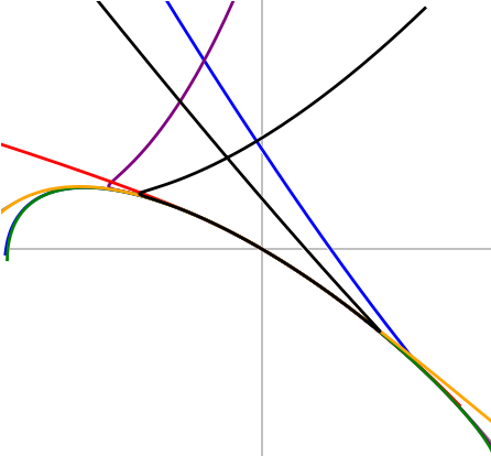
Figure 4. Six real $(4,4)$-interpolants

Here, $s_{3},\ldots,s_{8}$ define real curves. Figure 4 plots their branches near $t=0$.

References

- [1] Daniel J. Bates, Jonathan D. Hauenstein, Andrew J. Sommese, and Charles W. Wampler. Bertini: Software for numerical algebraic geometry. Available at bertini.nd.edu with permanent doi: dx.doi.org/10.7274/R0H41PB5.
- [2] C. de Boor, K. Hollig, and M. Sabin. High accuracy geometric hermite interpolation. Computer Aided Geometric Design, 4:269–278, December 1987.
- [3] Taylor Brysiewicz. Lower bounds on the number of real polynomially parametrized interpolants. Available at http://www.math.tamu.edu/t̃brysiewicz/realInterpolants.
- [4] Daniel R. Grayson and Michael E. Stillman. Macaulay2, a software system for research in algebraic geometry. Available at http://www.math.uiuc.edu/Macaulay2/.
- [5] Elizabeth Gross, Jose Israel Rodriguez, Dan Bates, and Anton Leykin. Bertini: Interface to Bertini. Version 2.1.2.3. Available at https://github.com/Macaulay2/M2/tree/master/M2/Macaulay2/packages.
- [6] Jonathan D. Hauenstein and Frank Sottile. alphacertified. Available at http://www4.ncsu.edu/~jdhauens/alphaCertified/.
- [7] K. Höllig and J. Koch. Geometric hermite interpolation with maximal order and smoothness. Computer Aided Geometric Design, 13(8):681–695, 1996.
- [8] G. Jaklic, J. Kozak, M. Krajnc, and E. Zagar. On geometric interpolation by planar parametric polynomial curves. Mathematics of Computation, 76:1981–1993, 2007.
- [9] G. Jaklic, J. Kozak, M. Krajnc, and E. Zagar. On geometric interpolation of circle-like curves. Computer Aided Geometric Design, 24:241–251, 2007.
- [10] Edgar Palmer and Allen Schwenk. The number of self complementary achiral necklaces. Journal of Graph Theory, 1:309 – 315, 10 2006.
- [11] A. Rababah. Taylor theorem for planar curves. Proceedings American Mathematical Society, page 119(3):803.810, 1993.
- [12] K. Scherer. Parametric polynomial curves of local approximation order 8. Curves and Surface Fitting, pages 375–384, 2003.
- [13] Igor Shafarevich. Basic Algebraic Geometry 1: Varieties in Projective Space. Springer, 3rd edition, 1974.
- [14] N. J. A. Sloane. The on-line encyclopedia of integer sequences. Published electronically at https://oeis.org.
- [15] S. Smale. Newton’s method estimates from data at one point. The merging of disciplines: new directions in pure, applied, and computational mathematics (Laramie, Wyo., 1985), pages 37–51, 1986.