Approximating tau-functions by theta-functions

Abstract

We prove that the logarithm of an arbitrary tau-function of the KdV hierarchy can be approximated, in the topology of graded formal series by the logarithmic expansions of hyperelliptic theta-functions of finite genus, up to at most quadratic terms. As an example we consider theta-functional approximations of the Witten–Kontsevich tau-function.

1 Introduction

Consider the algebra ${\mathcal{W}}=\mathbb{C}[{\bf a},{\bf b},{\bf c}]$ of polynomials in infinite number of variables

$${\bf a}=(a_{1},a_{2},\dots),\quad{\bf b}=(b_{1},b_{2},\dots),\quad{\bf c}=(c_{1},c_{2},\dots).$$

Define a gradation on ${\mathcal{W}}$ by

$$\deg a_{i}=2i+1,\quad\deg b_{i}=\deg c_{i}=2i.$$ (1.1)

Introduce the matrix-valued formal Laurent series in $1/z$

$$W(z)\equiv W({\bf a},{\bf b},{\bf c};z)=\left(\begin{array}[]{cc}0&1\\ z+c_{1}&0\end{array}\right)+\sum_{i\geq 1}\left(\begin{array}[]{cc}a_{i}&b_{i}\\ c_{i+1}&-a_{i}\end{array}\right)\frac{1}{z^{i}}$$ (1.2)

and define a Poisson algebra structure on ${\mathcal{W}}$ by means of the following Poisson bracket

$$\left\{W(z_{1})\underset{,}{\otimes}W(z_{2})\right\}=\left(\left[R(z_{1}-z_{2}),W(z_{1})\otimes{\bf 1}+{\bf 1}\otimes W(z_{2})\right]\right)_{-}+\left[\Delta R,W(z_{1})\otimes{\bf 1}-{\bf 1}\otimes W(z_{2})\right]$$ (1.3)

where

$$R(z)=\frac{P}{z}$$ (1.4)

is the standard $r$-matrix,

$$P:\mathbb{C}^{2}\otimes\mathbb{C}^{2}\to\mathbb{C}^{2}\otimes\mathbb{C}^{2},\quad P(x\otimes y)=y\otimes x$$

and

$$\Delta R=E_{21}\otimes E_{21}\quad\text{with}\quad E_{21}=\left(\begin{array}[]{cc}0&0\\ 1&0\end{array}\right).$$ (1.5)

For any pair of homogeneous elements $f,\,g\in{\mathcal{W}}$ one has

$$\deg\{f,g\}=\deg f+\deg g-3.$$ (1.6)

The annihilator of the Poisson bracket coincides with the subring $\mathbb{C}[b_{1}+c_{1}]$.

We will now introduce an infinite family of derivations on the algebra ${\mathcal{W}}$. Let

$$Q(z)=-\det W(z)=z+\sum_{i\geq 1}\frac{q_{i}}{z^{i-1}}.$$ (1.7)

Define an infinite sequence of polynomials $H_{n}\in{\mathcal{W}}$,  $n\geq-1$ using coefficients of the following series

$$1+\frac{1}{2}\sum_{n\geq-1}\frac{H_{n}}{z^{n+2}}=\sqrt{\frac{Q(z)}{z}}.$$ (1.8)

The polynomial $H_{-1}=b_{1}+c_{1}$ is the Casimir of the Poisson bracket. The derivations $\partial_{n}$ are defined as Hamiltonian vector fields

$$\partial_{n}f=\{H_{n},f\}\quad\forall\,f\in{\mathcal{W}},\quad n\geq 0.$$ (1.9)

Explicitely

$$\partial_{0}=\left(c_{2}-b_{2}+b_{1}^{2}-b_{1}c_{1}\right)\frac{\partial}{\partial a_{1}}-2a_{1}\frac{\partial}{\partial b_{1}}+2a_{1}\frac{\partial}{\partial c_{1}}+$$

$$+\left(c_{3}-b_{3}+b_{2}(b_{1}-c_{1})\right)\frac{\partial}{\partial a_{2}}-2a_{2}\frac{\partial}{\partial b_{2}}+2\left(a_{2}+a_{1}(c_{1}-b_{1})\right)\frac{\partial}{\partial c_{2}}+\dots$$

$$\partial_{1}=\left(c_{3}-b_{3}+\frac{1}{2}b_{2}(3b_{1}-c_{1})-\frac{1}{2}c_{2}(b_{1}+c_{1})-\frac{1}{2}b_{1}(b_{1}^{2}-c_{1}^{2})\right)\frac{\partial}{\partial a_{1}}+\left(-2a_{2}+a_{1}(b_{1}+c_{1})\right)\frac{\partial}{\partial b_{1}}+$$

$$+\left(2a_{2}+a_{1}(b_{1}+c_{1})\right)\frac{\partial}{\partial c_{1}}+\left(c_{4}-b_{4}+\frac{1}{2}(b_{3}+c_{3})(b_{1}-c_{1})-\frac{1}{2}b_{2}(2c_{2}-2b_{2}+b_{1}^{2}-c_{1}^{2}\right)\frac{\partial}{\partial a_{2}}+$$

$$+\left(-2a_{3}+a_{2}(c_{1}-b_{1})+2a_{1}b_{2}\right)\frac{\partial}{\partial b_{2}}+\left(2a_{3}+a_{2}(c_{1}-b_{1})-2a_{1}b_{2}+a_{1}(b_{1}^{2}-a_{1}^{2})\right)\frac{\partial}{\partial c_{2}}+\dots$$

etc. Note that the Hamiltonian $H_{n}$ is a graded homogeneous polynomial of degree $2n+4$. Thus the derivation $\partial_{n}$ increases the degree by $2n+1$.

We will now derive a “commutator representation” for the action of the vector fields $\partial_{n}$ on $W(z)=W({\bf a},{\bf b},{\bf c},z)$. To this end introduce another matrix-valued series

$$M(z)\equiv M({\bf a},{\bf b},{\bf c};z)=\frac{W(z)}{\sqrt{Q(z)/z}}=\left(\begin{array}[]{cc}0&1\\ z&0\end{array}\right)+\sum_{i\geq 0}\left(\begin{array}[]{cc}\tilde{a}_{i}&\tilde{b}_{i}\\ \tilde{c}_{i+1}&-\tilde{a}_{i}\end{array}\right)\frac{1}{z^{i}}$$ (1.14)

$$\tilde{a}_{i},~{}\tilde{b}_{i},~{}\tilde{c}_{i}\in{\mathcal{W}},\quad\tilde{a}_{0}=\tilde{b}_{0}=0,\quad\tilde{c}_{1}=\frac{c_{1}-b_{1}}{2}.$$

Note that

$$\det M(z)=-z.$$

Lemma 1.1

For any $n\geq 0$ the following equation holds true

$$\partial_{n}W(z)=\left[U_{n}(z),W(z)\right],\quad n=0,\,1,\,2,\dots$$ (1.15)

where

$$U_{n}(z)=\left[z^{n+1}M(z)\right]_{+}-\left(\begin{array}[]{cc}0&0\\ \tilde{b}_{n+1}&0\end{array}\right).$$ (1.16)

Corollary 1.2

The derivations $\partial_{n}$ commute pairwise.

Remark 1.3

One can consider in a similar way the graded algebra ${\mathcal{W}}_{g}$ of polynomials in $3g+1$ variables

$${\mathcal{W}}_{g}=\mathbb{C}[a_{1},\dots,a_{g},b_{1},\dots,b_{g},c_{1},\dots,c_{g+1}].$$

A Poisson bracket on ${\mathcal{W}}_{g}$ defined by a formula similar to (1.3) first appeared in [10]. However it differs from the one induced by restriction of (1.3) wrt the natural embedding

$${\mathcal{W}}_{g}\subset{\mathcal{W}},\quad W(z)\mapsto\frac{1}{z^{g}}W(z).$$

Due to the commutativity of derivations $[\partial_{n},\partial_{m}]=0$ for an arbitrary triple of sequences of complex numbers $a_{i}^{0}$, $b_{i}^{0}$, $c_{i}^{0}$, $i\geq 1$ there exists a unique common solution

$$a_{i}({\bf t}),~{}b_{i}({\bf t}),~{}c_{i}({\bf t})\in\mathbb{C}[[t_{0},t_{1},\dots]],\quad i=1,\,2,\dots$$

to the following infinite system of Hamiltonian differential equations

$$\frac{da_{i}}{dt_{k}}=\partial_{k}a_{i},\quad\frac{db_{i}}{dt_{k}}=\partial_{k}b_{i},\quad\frac{dc_{i}}{dt_{k}}=\partial_{k}c_{i},\quad i=1,\,2,\dots,\quad k=0,\,1,\dots$$ (1.17)

satisfying the initial conditions

$$a_{i}(0)=a_{i}^{0},~{}b_{i}(0)=b_{i}^{0},~{}c_{i}(0)=c_{i}^{0},\quad i=1,\,2,\dots$$

We will now establish a relationship between this infinite system of commuting polynomial ODEs with the Korteweg–de Vries (KdV) hierarchy of PDEs

$$u_{t_{0}}=u_{x}$$

$$u_{t_{1}}=3u\,u_{x}+\frac{1}{4}u_{xxx}$$ (1.18)

$$u_{t_{2}}=\frac{15}{2}u^{2}u_{x}+\frac{5}{2}\left(2u_{x}u_{xx}+u\,u_{xxx}\right)+\frac{1}{16}u^{(5)}$$

etc. that can be represented in the Lax form

$$\frac{\partial}{\partial t_{n}}L=\left[\left(L^{\frac{2n+1}{2}}\right)_{+},\,L\right],\quad L=\partial_{x}^{2}+2u.$$

Consider the matrix-valued series

$$W^{0}(z)=\left(\begin{array}[]{cc}0&1\\ z+c_{1}^{0}&0\end{array}\right)+\sum_{i\geq 1}\left(\begin{array}[]{cc}a_{i}^{0}&b_{i}^{0}\\ c_{i+1}^{0}&-a_{i}^{0}\end{array}\right)\frac{1}{z^{i}}.$$

For any $N\geq 2$ define a collection of numbers $F^{0}_{k_{1}\dots k_{N}}$ labelled by indices $k_{1}$, …, $k_{N}=0,\,1,\dots$ by the following generating series

$$\sum_{k_{1},\dots,k_{N}}\frac{F^{0}_{k_{1}\dots k_{N}}}{z_{1}^{k_{1}+1}\dots z_{N}^{k_{N}+1}}=$$ (1.19)

$$=-\frac{1}{N}\frac{1}{\sqrt{\frac{Q(z_{1})}{z_{1}}}\dots\sqrt{\frac{Q(z_{N})}{z_{N}}}}\sum_{s\in S_{N}}\frac{{\rm tr}\left[W^{0}(z_{s_{1}})\dots W^{0}(z_{s_{N}})\right]}{(z_{s_{1}}-z_{s_{2}})\dots(z_{s_{N-1}}-z_{s_{N}})(z_{s_{N}}-z_{s_{1}})}-\delta_{N,2}\frac{z_{1}+z_{2}}{(z_{1}-z_{2})^{2}}.$$

Define a function $F({\bf t})\in\mathbb{C}[[{\bf t}]]$ by its formal Taylor series expansion

$$F({\bf t})=\sum_{N\geq 2}\frac{1}{N!}\sum_{k_{1},\dots,k_{N}}F^{0}_{k_{1}\dots k_{N}}t_{k_{1}}\dots t_{k_{N}}.$$ (1.20)

Theorem 1.4

For arbitrary initial conditions $a_{i}^{0}$, $b_{i}^{0}$, $c_{i}^{0}$ the function

$$u({\bf t})=\frac{\partial^{2}F({\bf t})}{\partial t_{0}^{2}}$$

satisfies equations of the KdV hierarchy. The tau-function of this solution is equal to

$$\tau({\bf t})=e^{F({\bf t})}$$

up to a transformation $\tau({\bf t})\mapsto e^{\alpha+\sum\beta_{i}t_{i}}\tau({\bf t})$ with some constant coefficients $\alpha$, $\beta_{i}$. Any solution $u({\bf t})\in\mathbb{C}[[{\bf t}]]$ of the KdV hierarchy along with its tau-function can be obtained by this procedure.

Remark 1.5

Changing $W(z)$ by a scalar factor

$$W(z)\mapsto f(z)\,W(z),\quad f(z)=1+\sum_{i\geq 1}\frac{f_{i}}{z^{i}}\in\mathbb{C}[[1/z]]$$

does not change the KdV solution.

Note that the polynomial $F_{i_{1}\dots i_{N}}({\bf a},{\bf b},{\bf c})=\partial^{N}\log\tau/\partial t_{i_{1}}\dots\partial t_{i_{N}}$ defined by eq. (1.19) is graded homogeneous of the degree $2(i_{1}+\dots+i_{N})+N$. Therefore it belongs to the subring ${\mathcal{W}}_{g}=\mathbb{C}[a_{1},\dots,a_{g},$ $b_{1},\dots,b_{g},c_{1},\dots,c_{g+1}]$ for

$$g=i_{1}+\dots+i_{N}+\left[\frac{N}{2}\right].$$

We can reformulate this observation in the following way.

Let

$$f({\bf t})=\sum_{n\geq 0}\frac{1}{n!}\sum_{i_{1},\dots,i_{n}}f_{i_{1}\dots i_{n}}t_{i_{1}}\dots t_{i_{n}}\in\mathbb{C}[[{\bf t}]]$$

be a formal series of an infinite number of variables ${\bf t}=(t_{0},t_{1},\dots)$. For a given number $m>0$ denote

$$\left[f({\bf t})\right]_{m}=\sum_{n\geq 0}\frac{1}{n!}\sum_{2(i_{1}+\dots+i_{n})+n\leq m}f_{i_{1}\dots i_{n}}t_{i_{1}}\dots t_{i_{n}}$$ (1.21)

the $m$-truncation of the series.

Corollary 1.6

Let $\tau({\bf t})$ be the tau-function of an arbitrary solution $u({\bf t})\in\mathbb{C}[[{\bf t}]]$ of the KdV hierarchy. Then for any $m>0$ there exists a hyperelliptic curve $C$ of genus less or equal than $\left[\frac{m}{2}\right]$ and a point ${\bf u}_{0}\in J(C)\setminus\left(\Theta\right)$ in the Jacobian such that

$$\left[\log\tau({\bf t})\right]_{m}=\left[\log\theta\left(\sum_{2i+1\leq m}t_{i}{\bf V}^{(i)}-{\bf u}_{0}\right)\right]_{m}+\alpha+\sum_{2i+1\leq m}\beta_{i}t_{i}+\frac{1}{2}\sum_{2(i+j+1)\leq m}\gamma_{ij}t_{i}t_{j}$$

for some constants $\alpha$, $\beta_{i}$, $\gamma_{ij}$.

Remark 1.7

It can happen that the curve $C$ is singular. In that case one has to deal with the generalized Jacobian and the corresponding analogue of theta-function.

Our last remark is about a block-triangular invertible change of variables between the generators of the algebra ${\mathcal{W}}$ and the jet variables $u$, $u_{x}$, …depending on the constants of motion $q_{i}$ (see eq. (1.7))

$$\{a_{1},b_{1},c_{1},\dots,a_{n},b_{n},c_{n}\}\leftrightarrow\{f_{2},\dots,f_{2n+1},q_{1},\dots,q_{n}\}$$ (1.22)

for every $n\geq 1$. Here

$$f_{2}=\frac{1}{2}(b_{1}-c_{1})=\left(\log\tau\right)_{00}=u,\quad f_{3}=\left(\log\tau\right)_{000}=u_{x},\dots,f_{2n+1}=\partial_{0}^{2n+1}\log\tau=u^{(2n-1)}.$$

Explicitly

$$a_{1}=-\frac{1}{2}u_{x},\quad b_{1}=u+\frac{1}{2}q_{1},\quad c_{1}=-u+\frac{1}{2}q_{1}$$

$$a_{2}=-\frac{1}{8}u_{xxx}-\frac{3}{2}u\,u_{x}-\frac{1}{4}q_{1}u_{x},\quad b_{2}=\frac{1}{4}u_{xx}+\frac{3}{2}u^{2}+\frac{1}{2}q_{1}u+\frac{q_{2}}{2}-\frac{q_{1}^{2}}{2},\quad c_{2}=-\frac{1}{4}u_{xx}-\frac{1}{2}u^{2}-\frac{1}{2}q_{1}u+\frac{q_{2}}{2}-\frac{q_{1}^{2}}{2}$$

etc. After such a change the matrix polynomials $U_{n}(z)$ take the familiar form

$$U_{0}=\left(\begin{array}[]{cc}0&1\\ z-2u&0\end{array}\right),\quad U_{1}=\left(\begin{array}[]{cc}-\frac{u_{x}}{2}&z+u\\ z^{2}-u\,z-\frac{u_{xx}}{2}-2u^{2}&\frac{u_{x}}{2}\end{array}\right)$$

etc. Observe that the coefficients of these matrix polynomials depend only on the jet variables but not on the integration constants $q_{i}$.

The constructions of the present paper can be generalized to other spaces of matrix-valued series. Moreover they can be extended to series with coefficients in an arbitrary simple Lie algebra. This will be done in a separate publication.

2 Proofs

We begin with the proof of Lemma 1.1. Let us rewrite the Poisson bracket (1.3) in coordinates,

$$\{a(z),a(w)\}=0,\quad\{a(z),b(w)\}=-\frac{b(z)-b(w)}{z-w},\quad\{a(z),c(w)\}=\frac{c(z)-c(w)}{z-w}-b(z)$$

$$\{b(z),b(w)\}=0,\quad\{b(z),c(w)\}=-2\frac{a(z)-a(w)}{z-w},\quad\{c(z),c(w)\}=2[a(z)-a(w)]$$ (2.1)

where we denote

$$a(z)=\sum_{i\geq 1}\frac{a_{i}}{z^{i}},\quad b(z)=\sum_{i\geq 1}\frac{b_{i}}{z^{i}},\quad c(z)=\sum_{i\geq 1}\frac{c_{i}}{z^{i-1}}.$$

Using (2) obtain

$$\left\{Q(w),W(z)\right\}\equiv\left(\begin{array}[]{lr}\{Q(w),a(z)\}&~{}\{Q(w),b(z)\}\\ \{Q(w),c(z),\}&-\{Q(w),a(z)\}\end{array}\right)=\frac{1}{w-z}\left[W(w),W(z)\right]-b(w)\left[E_{21},W(z)\right].$$

Thus

$$\left\{\sum_{n\geq-1}\frac{H_{n}}{w^{n+1}},W(z)\right\}=2w\left\{\sqrt{\frac{Q(w)}{w}},W(z)\right\}=\frac{1}{w-z}\left[M(w),W(z)\right]-\tilde{b}(w)\left[E_{21},W(z)\right]$$ (2.2)

where

$$\tilde{b}(w)=\sum_{i\geq 1}\frac{b_{i}}{z^{i}}.$$

Collecting the coefficient of $w^{-n-1}$ in eq. (2.2) we obtain (1.15).    

Proof of Corollary 1.2. Due to the commutator structure of the rhs of eq. (2.2) we deduce that

$$\left\{\sum_{n\geq-1}\frac{H_{n}}{w^{n+1}},\det W(z)\right\}=0$$

hence

$$\left\{\sum_{n\geq-1}\frac{H_{n}}{w^{n+1}},\sum_{m\geq-1}\frac{H_{m}}{z^{m+1}}\right\}=0.$$

   

Proof of Theorem 1.4. Introduce a ${\bf t}$-dependent matrix series

$$W({\bf t},z):=W\left({\bf a}({\bf t}),{\bf b}({\bf t}),{\bf c}({\bf t}),z\right)$$

and

$$M({\bf t},z):=M\left({\bf a}({\bf t}),{\bf b}({\bf t}),{\bf c}({\bf t}),z\right)=\frac{W({\bf t},z)}{\sqrt{Q(z)/z}}.$$

Due to Lemma 1.1 the matrix series $W({\bf t},z)$ satisfies

$$\frac{d}{dt_{n}}W({\bf t},z)=\left[U_{n}({\bf t},z),W({\bf t},z)\right],\quad n\geq 0$$

where the matrix polynomials $U_{n}({\bf t},z)$ are obtained from the series $M({\bf t},z)$ by the construction of eq. (1.16). In particular,

$$U_{0}({\bf t},z)=\left(\begin{array}[]{cc}0&1\\ z-2u({\bf t})&0\end{array}\right),\quad u({\bf t}):=\frac{1}{2}(b_{1}({\bf t})-c_{1}({\bf t})).$$ (2.3)

Similar equations hold true for $M({\bf t},z)$

$$\frac{d}{dt_{n}}M({\bf t},z)=\left[U_{n}({\bf t},z),M({\bf t},z)\right],\quad n\geq 0$$

Because of the commutativity of the derivations the matrix polynomials $U_{n}({\bf t},z)$ satisfy the “zero curvature equations”

$$\left[\frac{d}{dt_{n}}-U_{n}({\bf t},z),\frac{d}{dt_{m}}-U_{m}({\bf t},z)\right]=0\quad\forall~{}m,\,n\geq 0$$

that imply equations of the KdV hierarchy (1.18) for the function $u({\bf t})$.

To compute the tau-function of this solution, according to the recipe of [1] we have to find the so-called matrix resolvent, i.e. the unique matrix series $R({\bf t},z)$ of the form

$$R({\bf t},z)=\left(\begin{array}[]{cc}0&1\\ z-u({\bf t})&0\end{array}\right)+{\mathcal{O}}\left(\frac{1}{z}\right)$$

satisfying the equations

$$\frac{d}{dt_{n}}R({\bf t},z)=\left[U_{n}({\bf t},z),R({\bf t},z)\right],\quad n\geq 0$$

along with the normalization

$${\rm tr}\,R({\bf t},z)=0,\quad\det R({\bf t},z)=-z.$$

Then the $N$-th order logarithmic derivatives

$$F_{k_{1}\dots k_{N}}({\bf t}):=\frac{\partial^{N}\log\tau({\bf t})}{\partial t_{k_{1}}\dots\partial t_{k_{N}}}$$

of the tau-function of this solution for any $N\geq 2$ can be determined from the following generating series

$$\sum_{k_{1},\dots,k_{N}}\frac{F_{k_{1}\dots k_{N}}({\bf t})}{z_{1}^{k_{1}+1}\dots z_{N}^{k_{N}+1}}=-\frac{1}{N}\sum_{s\in S_{N}}\frac{{\rm tr}\left[R({\bf t},z_{s_{1}})\dots R({\bf t},z_{s_{N}})\right]}{(z_{s_{1}}-z_{s_{2}})\dots(z_{s_{N-1}}-z_{s_{N}})(z_{s_{N}}-z_{s_{1}})}-\delta_{N,2}\frac{z_{1}+z_{2}}{(z_{1}-z_{2})^{2}}.$$ (2.4)

Clearly the matrix series $M({\bf t},z)$ satisfies all these conditions, so $R({\bf t},z)=M({\bf t},z)$. Therefore the logarithmic derivatives of the tau-function of the solution $u({\bf t})$ are given by

$$\sum_{k_{1},\dots,k_{N}}\frac{F_{k_{1}\dots k_{N}}({\bf t})}{z_{1}^{k_{1}+1}\dots z_{N}^{k_{N}+1}}=$$

$$=-\frac{1}{N}\frac{1}{\sqrt{\frac{Q(z_{1})}{z_{1}}}\dots\sqrt{\frac{Q(z_{N})}{z_{N}}}}\sum_{s\in S_{N}}\frac{{\rm tr}\left[W({\bf t},z_{s_{1}})\dots W({\bf t},z_{s_{N}})\right]}{(z_{s_{1}}-z_{s_{2}})\dots(z_{s_{N-1}}-z_{s_{N}})(z_{s_{N}}-z_{s_{1}})}-\delta_{N,2}\frac{z_{1}+z_{2}}{(z_{1}-z_{2})^{2}},$$

$N\geq 2$. For ${\bf t}=0$ it reduces to eq. (1.20). This completes the proof of the first part of the theorem.

Converesely, let $u({\bf t})\in\mathbb{C}[[{\bf t}]]$ be a solution to the equations of the KdV hierarchy. Let $R({\bf t},z)\in Mat_{2}\left(\mathbb{C}[[{\bf t}]]\right)\otimes z\mathbb{C}[[1/z]]$ be the matrix resolvent of this solution. Put $W^{0}(z):=R(0,z)$. Then $Q(z)=z$ so eq. (2.4) at ${\bf t}=0$ coincides with (1.20).    

3 Examples

3.1 Logarithmic expansions of hyperelliptic theta-functions

Let us briefly revisit the finite-gap case within the general framework. Consider the subspace of matrix series that truncate at the $g$-th term,

$$W(z)\equiv W({\bf a},{\bf b},{\bf c};z)=\left(\begin{array}[]{cc}0&1\\ z+c_{1}&0\end{array}\right)+\sum_{i=1}^{g}\left(\begin{array}[]{cc}a_{i}&b_{i}\\ c_{i+1}&-a_{i}\end{array}\right)\frac{1}{z^{i}}.$$

It corresponds to the subalgebra

$${\mathcal{W}}_{g}=\mathbb{C}[a_{1},\dots,a_{g},b_{1},\dots,b_{g},c_{1},\dots,c_{g+1}]\subset{\mathcal{W}}$$

(we use the same notation as in Remark 1.3). Using the degree counting (1.6) it is easy to verify that ${\mathcal{W}}_{g}$ is a Poisson subalgebra wrt the Poisson bracket (1.3). The annihilator of the restriction of (1.3) onto ${\mathcal{W}}_{g}$ is generated by $g+1$ Casimirs $q_{1}=b_{1}+c_{1}$ and

$$q_{g+k+1}=\sum_{i=k}^{g}(a_{i}a_{g+k-i}+b_{i}c_{g+k+1-i}),\quad k=1,\dots,g.$$

The Darboux coordinates $x_{1},\dots,x_{g}$, $p_{1}$, …, $p_{g}$,

$$\{x_{i},x_{j}\}=\{p_{i},p_{j}\}=0,\quad\{p_{i},x_{j}\}=\delta_{ij}$$

on the symplectic leaves

$$q_{1}=q_{1}^{0},~{}q_{g+2}=q_{g+2}^{0},\dots,q_{2g+1}=q_{2g+1}^{0}$$

are obtained by the standard, see e.g. [11], up to a change $z\mapsto 1/z$ procedure by taking the $z$- and $w$-coordinates of poles of the eigenvector of the matrix $W(z)$. I.e., $x_{1}$, …, $x_{g}$ are roots of the equation

$$1+\frac{b_{1}}{z}+\dots+\frac{b_{g}}{z^{g}}=0$$

and

$$p_{i}=-\left(\frac{a_{1}}{x_{i}}+\dots+\frac{a_{g}}{x_{i}^{g}}\right),\quad i=1,\dots,g.$$

The corresponding solutions to the KdV hierarchy are often called finite-gap or algebro-geometric solutions. For them the tau-function coincides with the hyperelliptic theta-function up to multiplication by exponential of a quadratic polynomial. Let us recall this construction. It is convenient to change

$$W(z)\mapsto z^{g}W(z)$$

in order to deal with matrix polynomials of the form

$$W(z)=\left(\begin{array}[]{cc}a(z)&b(z)\\ c(z)&-a(z)\end{array}\right)$$ (3.3)

$$a(z)=a_{1}z^{g-1}+\dots+a_{g},\quad b(z)=z^{g}+b_{1}z^{g-1}+\dots+b_{g},\quad c(z)=z^{g+1}+c_{1}z^{g}+\dots+c_{g+1}.$$

Assuming the roots of

$$Q(z)=-\det W(z)=z^{2g+1}+q_{1}z^{2g}+\dots+q_{2g+1}$$

to be pairwise distinct we obtain a hyperelliptic curve $C$

$$w^{2}=z^{2g+1}+q_{1}z^{2g}+\dots+q_{2g+1}$$ (3.4)

of genus $g$ with one branch point $P_{\infty}$ at infinity. The fibers of the natural fibration

$$\begin{array}[]{c}\{{\rm space~{}of~{}matrix~{}polynomials}~{}W(z)=\left(\begin{array}[]{cc}0&z^{g}\\ z^{g+1}+c_{1}z^{g}&0\end{array}\right)+\dots+\left(\begin{array}[]{cc}a_{g}&b_{g}\\ c_{g+1}&-a_{i}\end{array}\right)\}\\ \Big{\downarrow}\\ \{{\rm space~{}of~{}hyperelliptic~{}curves}~{}w^{2}=z^{2g+1}+\dots+q_{2g+1}\}\end{array}$$

$$W(z)\mapsto\det(W(z)-w\cdot{\bf 1})=w^{2}-Q(z)$$ (3.5)

are isomorphic to the affine Jacobians $J(C)\setminus(\Theta)$ of the curves. Here $(\Theta)\subset J(C)$ is the theta divisor. For $g=1$ it comes from an easy calculation. For $g\geq 2$ it was first observed in [5], see also the book [9]. The correspondence between the matrices in the fibers of the fibration (3.5) can be established by the map

$$W(z)\mapsto\text{line bundle over}~{}C~{}\text{of eigenvectors of}~{}W(z).$$

The degree of the line bundle equals $g+1$. It is convenient to choose a representative in the class of linear equivalence in the form $D_{0}+P_{\infty}$ where

$$D_{0}=Q_{1}+\dots+Q_{g},\quad Q_{j}=(z_{j},w_{j})\in C\setminus P_{\infty}$$ (3.6)

is a nonspecial positive divisor of degree $g$ defined by the equations

$$b(z_{j})=0,\quad w_{j}=-a(z_{j}),\quad j=1,\dots,g.$$ (3.7)

Applying to the divisor $D_{0}$ the Abel–Jacobi map one obtains a point ${\bf u}_{0}\in J(C)\setminus(\Theta)$. Explicitely,

$${\bf u}_{0}=\sum_{j=1}^{g}\left(\int_{P_{\infty}}^{Q_{j}}\omega_{1},\dots,\int_{P_{\infty}}^{Q_{j}}\omega_{g}\right)-{\boldsymbol{\varpi}}$$ (3.8)

where

$$\omega_{i}=(\alpha_{i1}z^{g-1}+\dots+\alpha_{ig})\frac{dz}{2w},\quad i=1,\dots,g$$ (3.9)

are the normalized holomorphic differentials,

$$\oint_{a_{j}}\omega_{i}=2\pi\sqrt{-1}\,\delta_{ij}$$

for some basis $a_{1}$, …, $a_{g}$, $b_{1}$, …, $b_{g}\in H_{2}(C,\mathbb{Z})$,

$$a_{i}\circ a_{j}=b_{i}\circ b_{j}=0,\quad a_{i}\circ b_{j}=\delta_{ij}.$$

By $B_{ij}$ we will denote the matrix of $b$-periods of the normalized holomorphic differentials

$$B_{ij}=\oint_{b_{j}}\omega_{i},\quad i,\,j=1,\dots,g.$$

Recall that the Jacobi variety (or, simply Jacobian) of $C$ can be realized as a quotient of $\mathbb{C}^{g}$ over the lattice of periods of holomorphic differentials

$$J(C)=\mathbb{C}^{g}/\{2\pi\sqrt{-1}M+BN\,|\,M,\,N\in\mathbb{Z}^{g}\}$$

Finally, the half-period ${\boldsymbol{\varpi}}$, for a suitable choice of the basis of cycles (see details in [6]) has the form

$${\boldsymbol{\varpi}}=\pi\sqrt{-1}(1,0,1,0,\dots)+\frac{1}{2}\sum_{i=1}^{g}\left(B_{1i},B_{2i},\dots,B_{gi}\right).$$ (3.10)

Let

$$\theta({\bf u})=\sum_{{\bf n}\in\mathbb{Z}^{g}}\exp\left\{\frac{1}{2}\langle{\bf n},B{\bf n}\rangle+\langle{\bf n},{\bf u}\rangle\right\}$$ (3.11)

be the Riemann theta-function of the curve $C$ associated with the chosen basis of cycles. Here ${\bf u}=(u_{1},\dots,u_{g})$ is the vector of independent complex variables, ${\bf n}=(n_{1},\dots,n_{g})\in\mathbb{Z}^{g}$,

$$\langle{\bf n},B{\bf n}\rangle=\sum_{j,\,k=1}^{g}B_{jk}n_{j}n_{k},\quad\langle{\bf n},{\bf u}\rangle=\sum_{k=1}^{g}n_{k}u_{k}.$$

Then the tau-function of the solution to the KdV hierarchy corresponding to the the matrix (3.3) reads

$$\tau({\bf t})=e^{\frac{1}{2}\sum_{i,\,j\geq 0}q_{ij}t_{i}t_{j}}\theta\left(\sum t_{k}{\bf V}^{(k)}-{\bf u}_{0}\right)$$ (3.12)

where $\theta({\bf u})$ is the theta-function of the hyperelliptic curve (3.4), the point ${\bf u}_{0}$ is specified by eqs. (3.6)–(3.8), the vector ${\bf V}^{(k)}=\left(V^{(k)}_{1},\dots,V^{(k)}_{g}\right)$, $k\geq 0$ is made of the $b$-periods of the normalized second kind differentials

$$\Omega^{(k)}=\frac{2k+1}{2}\left(z^{g+k}+c_{k\,1}z^{g+k-1}+\dots+c_{k,g+k}\right)\frac{dz}{w}=$$

$$=\frac{1}{2}\left((2k+1)z^{k-\frac{1}{2}}+\sum_{i\geq 0}\frac{q_{k\,i}}{z^{i+\frac{3}{2}}}\right)\,dz,\quad k\geq 0$$ (3.13)

$$\oint_{a_{i}}\Omega^{(k)}=0,\quad V_{i}^{(k)}=\oint_{b_{i}}\Omega^{(k)},\quad i=1,\dots,g$$

and the coefficients $q_{ij}$ come from the regular part of the expansion (3.1). The vectors ${\bf V}^{(k)}$ can also be computed from the expansions of normalized holomorphic differentials

$$\omega_{i}=\frac{1}{2}\sum_{k\geq 0}V_{i}^{(k)}\frac{dz}{z^{k+\frac{3}{2}}},\quad i=1,\dots,g.$$ (3.14)

From Theorem 1.4 we derive

Corollary 3.1

The logarithmic derivatives of the theta-function of the hyperelliptic spectral curve (3.4) of the matrix polynomial $W(z)$ of the form (3.3) for any $N\geq 3$ satisfy the following identities

$$\sum_{k_{1},\dots,k_{N}\geq 0}\frac{\partial^{N}\log\theta\left(\sum t_{k}{\bf V}^{(k)}-{\bf u}_{0}\right)}{\partial t_{k_{1}}\dots\partial t_{k_{N}}}\Big{|}_{{\bf t}=0}\frac{1}{z_{1}^{k_{1}+\frac{3}{2}}\dots z_{N}^{k_{N}+\frac{3}{2}}}=$$

$$=-\frac{1}{N}\frac{1}{w(z_{1})\dots w(z_{N})}\sum_{s\in S_{N}}\frac{{\rm tr}\left[W\left(z_{s_{1}}\right)\dots W\left(z_{s_{N}}\right)\right]}{\left(z_{s_{1}}-z_{s_{2}}\right)\dots\left(z_{s_{N-1}}-z_{s_{N}}\right)\left(z_{s_{N}}-z_{s_{1}}\right)}$$ (3.15)

of formal series in inverse powers of independent variables $z_{1}^{1/2}$, …, $z_{N}^{1/2}$.

As an immediate consequence we obtain

Corollary 3.2

If (3.4) is the spectral curve of a matrix polynomial (3.3) with rational coefficients then the logarithmic derivatives

$$\frac{\partial^{N}\log\theta\left(\sum t_{k}{\bf V}^{(k)}-{\bf u}_{0}\right)}{\partial t_{k_{1}}\dots\partial t_{k_{N}}}\Big{|}_{{\bf t}=0}$$

of its theta-function evaluated at the point (3.6)–(3.8) are rational numbers for any $N\geq 3$.

Generalizations of this Corollary for more general spectral curves will be given in [4].

3.2 Theta-functional approximations of the Witten–Kontsevich tau-function

Let us consider the Airy operator

$$L=\frac{d^{2}}{dx^{2}}+2x.$$ (3.16)

Then the matrix resolvent computed in [1] has the form (1.2) with

$$a^{0}_{3k-2}=-\frac{1}{2}\frac{(6k-5)!!}{24^{k}(k-1)!},\quad b^{0}_{3k}=\frac{(6k-1)!!}{24^{k}k!},\quad c^{0}_{3k-1}=-\frac{6k+1}{6k-1}\frac{(6k-1)!!}{24^{k}k!},$$ (3.17)

all other coefficients vanish. Recall [1] that for this solution of the KdV hierarchy the logarithmic derivatives of the tau-function are related to the intersection numbers of the psi-classes in the cohomologies of the Deligne–Mumford moduli spaces of stable algebraic curves

$$F^{0}_{i_{1}\dots i_{N}}={\prod_{i=1}^{N}(2k_{i}+1)!!}\int_{\overline{M}_{g,N}}\psi_{1}^{k_{1}}\dots\psi_{N}^{k_{N}}$$

assuming

$$i_{1}+\dots+i_{N}-N+3=3g.$$

Let us consider for this particular case the procedure of approximation of $\log\tau({\bf t})$ by logarithms of theta-functions. As an example consider the 9-truncation of $F({\bf t})=\log\tau({\bf t})$

$$\left[F({\bf t})\right]_{9}=\frac{t_{1}}{24}+\frac{t_{4}}{1152}+\frac{t_{1}^{2}}{48}+\frac{t_{0}t_{2}}{16}+\frac{1}{6}t_{0}^{3}+\frac{1}{72}t_{1}^{3}+\frac{1}{12}t_{0}t_{1}t_{2}+\frac{1}{48}t_{0}^{2}t_{3}+\frac{1}{6}t_{0}^{3}t_{1}+\frac{1}{6}t_{0}^{3}t_{1}^{2}+\frac{1}{24}t_{0}^{4}t_{2}.$$ (3.18)

According to the Corollary this polynomial coincides, modulo the linear and quadratic terms with the 9-truncation of the Taylor logarithmic expansion of the genus 4 theta-function

$$\log\theta\left(t_{0}{\bf V}^{(0)}+\frac{1}{3}t_{1}{\bf V}^{(1)}+\frac{1}{15}t_{2}{\bf V}^{(2)}+\frac{1}{105}t_{3}{\bf V}^{(3)}+\frac{1}{945}t_{4}{\bf V}^{(4)}-{\bf u}_{0}\right)$$

of the spectral curve

$$w^{2}+\det W(z)=0,\quad W(z)=\left(\begin{array}[]{cc}-\frac{1}{2}z^{3}-\frac{35}{16}&z^{4}+\frac{5}{8}z\\ \\ z^{5}-\frac{7}{8}z^{2}&\frac{1}{2}z^{3}+\frac{35}{16}\end{array}\right),$$ (3.19)

see Figure 1. This immediately follows from Corollary 3.1. To be on the safe side we have checked this statement by a numerical computation of the theta-function. Some hints from [7] were helpful for us in this computation.

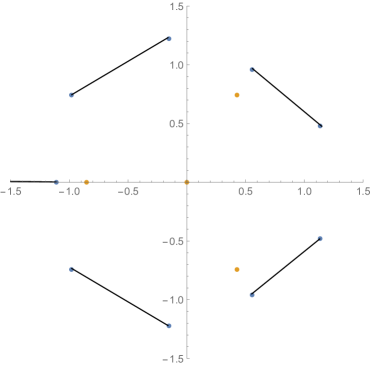
Figure 1: Branchcuts of the spectral curve (3.19). The yellow dots show the points $\left(0,\frac{35}{16}\right)$, $\left(-\frac{5^{1/3}}{2},\frac{15}{8}\right)$, $\left(-e^{2\pi i/3}\frac{5^{1/3}}{2},\frac{15}{8}\right)$, $\left(-e^{-2\pi i/3}\frac{5^{1/3}}{2},\frac{15}{8}\right)$ of the divisor $D_{0}$.

Choose the basis of cycles in the following way. The cycles $a_{1}$, …, $a_{4}$ go around the finite branch cuts. Every cycle $b_{i}$ crosses once the cycle $a_{i}$ and also the infinite branch cut. This yields the following matrix of $b$-periods of normalized holomorphic differentials

$$B=\left(\oint_{b_{j}}\omega_{i}\right)=-\left(\begin{array}[]{cccc}5.800&2.811&1.720&0.895\\ 2.811&7.374&3.263&1.722\\ 1.720&3.263&7.376&2.815\\ 0.895&1.722&2.815&5.807\\ \end{array}\right)+\sqrt{-1}\left(\begin{array}[]{cccc}1.272&1.842&2.376&3.137\\ 1.842&2.116&3.137&3.898\\ 2.376&3.137&4.158&4.431\\ 3.137&3.898&4.431&5.000\\ \end{array}\right)$$

where

$$\omega_{1}=\left[(-0.866+0.572\,i)z^{3}+(1.456\,+0.275\,i)z^{2}-(1.137\,+1.343\,i)z+(0.064\,+1.643\,i)\right]\frac{dz}{w}$$

$$\omega_{2}=\left[(-1.332+0.261\,i)z^{3}-(0.260\,-1.042\,i)z^{2}-(0.316\,-1.270\,i)z+(1.994\,+1.213\,i)\right]\frac{dz}{w}$$

$$\omega_{3}=\left[(-1.332-0.261\,i)z^{3}-(0.260\,+1.042\,i)z^{2}-(0.316\,+1.270\,i)z+(1.994\,-1.213\,i)\right]\frac{dz}{w}$$

$$\omega_{4}=\left[(-0.866-0.572\,i)z^{3}+(1.456\,-0.275\,i)z^{2}-(1.137\,-1.343\,i)z+(0.064\,-1.643\,i)\right]\frac{dz}{w}.$$

With the help of (3.14) we obtain the vectors ${\bf V}^{(k)}$

$${\bf V}^{(0)}=\left(-1.731+1.145\,i,-2.664+0.522\,i,-2.664-0.522\,i,-1.731-1.145\,i\right)$$

$${\bf V}^{(1)}=\left(2.912+0.551\,i,-0.520+2.083\,i,-0.520-2.083\,i,2.912-0.551\,i\right)$$

$${\bf V}^{(2)}=\left(-2.273-2.685\,i,-0.632+2.541\,i,-0.632-2.541\,i,-2.273+2.685\,i\right)$$

$${\bf V}^{(3)}=\left(0.127+3.286\,i,3.987+2.426\,i,3.987-2.426\,i,0.127-3.286\,i\right)$$

and ${\bf V}^{(4)}=0$. Finally, we compute the Abel–Jacobi image

$$\left(4.506+5.841\,i,6.826+1.741\,i,6.826-1.741\,i,4.506-5.841\,i\right)$$

of the divisor $D_{0}$ and the point ${\bf u}_{0}\in J(C)\setminus(\Theta)$

$${\bf u}_{0}=\left(10.119-1.614\,i,14.411-3.756\,i,14.413-11.933\,i,10.126-14.074\,i\right).$$

To avoid computational problems with big real parts it is convenient to shift this point by a vector of the lattice

$${\bf u}_{0}\mapsto{\bf u}_{0}+B(1,1,1,1).$$

Finally, we arrive at the following 9-truncated expansion

$$\left[\log\theta\left(t_{0}{\bf V}^{(0)}+\frac{1}{3}t_{1}{\bf V}^{(1)}+\frac{1}{15}t_{2}{\bf V}^{(2)}+\frac{1}{105}t_{3}{\bf V}^{(3)}+\frac{1}{945}t_{4}{\bf V}^{(4)}-{\bf u}_{0}\right)\right]_{9}=$$

$$=0.447+0.002\,i-(0.577+0.003\,i)t_{0}+0.186\,t_{1}+0.05\,t_{2}$$

$$+0.228\,t_{0}^{2}+0.175\,t_{0}t_{1}+0.07\,t_{1}^{2}+0.091\,t_{0}t_{2}-0.057\,t_{1}t_{2}-0.016\,t_{0}t_{3}$$

$$+0.167\,t_{0}^{3}+0.014\,t_{1}^{3}+0.084\,t_{0}t_{1}t_{2}+0.021\,t_{0}^{2}t_{3}+0.167\,t_{0}^{3}t_{1}+0.167\,t_{0}^{3}t_{1}^{2}+0.042\,t_{0}^{4}t_{2}.$$

We have omitted terms less than $10^{-3}$. Two small imaginary numbers in the first line come from some numerical errors to be settled. The first two lines are of no interest but the third line satisfactory matches the expansion (3.18) (the apparent discrepancy in the coefficient in front of $t_{0}t_{1}t_{2}$ is $\simeq 5\cdot 10^{-4}$).

Let us also make few comments about the theta-functional approximations of the Witten–Kontsevich tau-function for growing order of the truncation. For a given $g>0$ denote

$$W^{0}_{g}(z)=\left(\begin{array}[]{cc}0&1\\ z+c_{1}^{0}&0\end{array}\right)+\sum_{i=1}^{g}\left(\begin{array}[]{cc}a_{i}^{0}&b_{i}^{0}\\ c_{i+1}^{0}&-a_{i}^{0}\end{array}\right)\frac{1}{z^{i}}.$$

In order to compute the $m$-truncated $\log\tau({\bf t})$ with $m=2g$ or $m=2g+1$ according to Corollary one has to deal with the spectral curve of $W^{0}_{g}(z)$. Here we will consider one particular subfamily of spectral curves with $g=3n+1$. In that case there are $6n+3$ zeroes of the equation $\det W^{0}_{3n+1}(z)=0$ that, for large $n$ are distributed in the following way. One of them is on the real axis near $z=1$. Other zeros are located near two circles (see Figure 2 for $n=33$). On the inner circle there are $3n$ zeros and on the outer one there are $3n+2$ zeroes. The inner zeros are close to roots of the equation

$$1+\sum_{i=1}^{3n}\frac{b_{i}^{0}}{z^{i}}=0$$

while the outer poles are close to the roots of

$$z+\sum_{i=1}^{3n+2}\frac{c_{i}^{0}}{z^{i-1}}=0.$$

Taking into account only the leading terms of these equations one obtains the following asymptotics for the radii of these two circles for large $n$

$$\log R_{\rm in}\sim\frac{2}{3}(\log 3n-1)-\frac{\log n}{6n}+{\mathcal{O}}\left(\frac{1}{n}\right),\quad\log R_{\rm out}\sim\frac{2}{3}(\log 3n-1)+\frac{\log n}{18n}+{\mathcal{O}}\left(\frac{1}{n}\right)$$

so

$$\frac{R_{\rm out}}{R_{\rm in}}\sim n^{\frac{2}{9n}}.$$

The structure of the spectral curve for $g=3n+2$ is identical to the above one as $W^{0}_{3n+2}(z)=W^{0}_{3n+1}(z)$. For $g=3n$ the spectral curve has a double point at $z=0$. The branch points are still located near two circles, like for the above case $g=3n+1$ but there is no branch point near $z=1$. Appearance of this exceptional real branch point for $g=3n+1$ requires a better understanding.

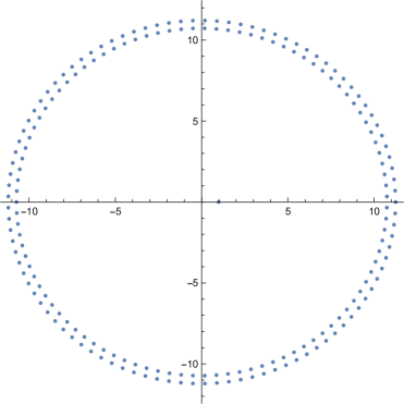
Figure 2: Branch points of the spectral curve of the matrix $W^{0}_{100}(z)$

SISSA, Via Bonomea, 265, Trieste, Italy

References

- [1] M.Bertola, B.Dubrovin, D.Yang (2016). Correlation functions of the KdV hierarchy and applications to intersection numbers over . Physica D: Nonlinear Phenomena, 327, 30–57.
- [2] M.Bertola, B.Dubrovin, D.Yang (2016). Simple Lie algebras and topological ODEs. IMRN rnw285.
- [3] M.Bertola, B.Dubrovin, D.Yang (2016). Simple Lie algebras, Drinfeld–Sokolov hierarchies, and multipoint correlation functions, arXiv:1610.07534.
- [4] B.Dubrovin (to appear). Algebraic spectral curves over and their tau-functions.
- [5] B.Dubrovin, S.P.Novikov, Periodic Korteweg–de Vries and Sturm–Liouville problems. Their connection with algebraic geometry. Sov. Math. Dokl. 219:3 (1974)
- [6] J.Fay. Theta-Functions on Riemann Surfaces. Springer Lecture Notes in Mathematics 352, 1973.
- [7] J.Frauendiener, C.Klein, Computational approach to hyperelliptic Riemann surfaces. Lett. Math. Phys. 105 (2015) 379-400.
- [8] I.M.Krichever, Methods of algebraic geometry in the theory of nonlinear equations. Russ. Math. Surveys 32 (1977) 183-208.
- [9] D.Mumford, Tata Lectures on Theta, vols, I, II. Birkhäuser, Boston (1983).
- [10] A.Nakayashiki, F.Smirnov, Cohomologies of Affine Jacobi Varieties and Integrable Systems, Comm. Math. Phys. 217 (2001) 623-652.
- [11] S.P.Novikov, A.P.Veselov, Poisson brackets compatible with algebraic geometry and Korteweg–de Vries dynamics on the set of finite zone potentials. Soviet Math. Doklady 26 (1982) 533-537.