Modified gravity versus shear viscosity: imprints on the scalar matter perturbations

Abstract

Cosmological scalar perturbation theory studied in the Newtonian gauge depends on two potentials $\Phi$ and $\Psi$. In General Relativity (GR) they must coincide ($\Phi=\Psi$) in the absence of anisotropic stresses sourced by the energy momentum tensor. On the other hand, it is widely accepted in the literature that potential deviations from GR can be parameterized by $\Phi\neq\Psi$. The latter feature is therefore present in both GR cosmologies equipped with shear viscous fluids or modified gravity. We study the evolution of scalar matter density perturbations using the redshift-space-distortion based $f(z)\sigma_{8}(z)$ data as a tool to differentiate and characterize the imprints of both scenarios. We show that in the $f(z)\sigma_{8}(z)$ evolution both scenarios yields to completely different imprints in comparison to the standard cosmology. While the current available data is not sensitive to distinguish modified gravity from viscous shear cosmologies, future precise data can be used to break this indistinguishability.

I Introduction

The several available cosmological observables powerfully constrain the background expansion of the universe as the one dictated by the flat-$\Lambda$CDM model, i.e., a GR based description for gravity composed of baryonic plus dark matter ($\Omega_{m0}\sim 0.3$) and a cosmological constant $\Lambda$ $(\Omega_{\Lambda}\sim 0.7)$. However, the background expansion, which can be characterized by the Hubble term evolution $H_{\Lambda}$ in the $\Lambda$CDM model, can also be achieved in modified gravity scenarios if suitable choices in their degrees of freedom are made. Therefore, investigation of the perturbative cosmological sector is necessary as an additional tool such as to increase our ability to distinguish GR from its possible candidate extensions.

The recent detection of gravitational waves from $GW170817$ Monitor:2017mdv has set the bound on the gravitational wave speed $c_{gw}$ compared to the light speed $c$ as $\left|c^{2}_{gw}/c^{2}-1\right|<5\times 10^{-15}$. This result severely reduces the available parameter space of generic Lorentz-breaking modifications of gravity, as for example some branches of the Horndeski (and Beyond-Horndeski) theory Creminelli:2017sry ; Ezquiaga:2017ekz . Hence, the radiative sector of gravitational theories seems to be tightly close to GR, but the potential sector could still have space to manifest some differences from the standard gravity.

Using the Newtonian gauge for cosmological scalar perturbations in an expanding, homogeneous and isotropic flat Universe, the line element reads

$$ds^{2}=a^{2}(\tau)\left[-(1+2\Phi)d\tau^{2}+(1-2\Psi)\delta_{ij}dx^{i}dx^{j}\right],$$ (1)

where $\tau$ is the conformal time and $\Phi$ and $\Psi$ are the metric perturbations. It is quite usual in the literature to parameterize phenomenological departures from GR in terms of a difference between the scalar potentials, $\Phi\neq\Psi$ (see, e.g., Ref. Ade:2015rim and references therein).

Apart from the perspective given above, the issue we want to stress out in this work is that $\Phi\neq\Psi$ is also naturally achieved in GR cosmologies if the energy-momentum tensor $T^{\mu\nu}$ of some of the energy components possesses anisotropic stresses like, e.g., shear viscosity. Then, we are left with the question: Is the possible inference of $\Phi\neq\Psi$ from observational data actually indicating a manifestation of modified gravity or would it be due to some non-conventional aspect of the universe’s energy content? In order to investigate this question we develop scalar perturbations in two different cosmologies, namely, i) GR gravity equipped with a cosmological constant and viscous (shear) matter and ii) modified gravity theories via usual parameterizations of the Poisson equation. Then, we compare the predictions for the growth of matter perturbations via the redshift-space-distortion based $f(z)\sigma_{8}(z)$ measurements Song:2008qt . In order to probe only the perturbative sector of these two approaches we will assume that both share the same background expansion as the one given by the standard flat-$\Lambda$CDM model. To some extent, similar strategies have been employed in Ref. Ade:2015rim ; Perenon:2015sla .

Shear viscous effects in cosmology are in fact receiving interest in the recent literature as a possible way of understanding different physical phenomena that might be in play both in the late universe Barbosa:2017ojt ; Thomas:2016iav ; Kopp:2016mhm ; Anand:2017wsj as also in the early universe BasteroGil:2011xd ; Bastero-Gil:2014jsa . These recent interests on shear viscous effects show that there are clear motivations for a deeper study of their possible effects and relevance in cosmology, which might eventually also provide relevant information about the nature of the dark matter itself. In the present work, our focus on the shear viscous effects is directly connected on how they contribute at the perturbation level and the issue of having $\Phi\neq\Psi$ for the gravitational perturbed potentials as a consequence of the presence of a nonvanishing shear viscosity. Our main interest then is to understand how this compares with the apparent similar situation in the context of modified gravity models, quantifying the possible differences in the two cases.

Among all possible viscous effects that could also affect the cosmological expansion, bulk viscosity is also very representative in the literature Zimdahl:1996ka . Here, we neglect this effect in a first approximation since it does not lead to $\Phi\neq\Psi$ contribution and this could also add an undesirable degenerescence in the proposed comparison between viscous effects and modified gravity. Also, bulk viscosity modifies the background expansion. This would place some difficulties in the strategy we want to promote here since it would be impossible to set the same background evolution for both scenarios (viscous cosmology and modified gravity). However, in spite of the degeneracy in introducing bulk viscosity, kinetic pressure and baryons effects, we estimate their impact in our analysis in general lines. We reinforce such aspects with the discussion presented in section V.

This paper is organized as follows. In section II we develop the perturbation dynamics of the model with shear viscosity. For this analysis, we take particular advantage of the results obtained in Ref. Barbosa:2017ojt , where we have placed an upper bound on the magnitude of dark matter shear viscosity allowed by the matter clustering observations. In section III, we develop the perturbed scalar equations for the case of modified gravity and present the parameterizations that will be used in this work. In section IV, we give our analysis of the quantitative comparison between the GR plus shear viscosity case and contrast these results with the modified gravity one by making use of the evolution of the $f\sigma_{8}$ observable. Finally, in section VI we give our conclusions.

II Dynamics of the viscous (shear) dark matter model

We start by focusing on the $\Lambda$CDM model and by assuming that matter behaves as a viscous/dissipative component possessing shear viscosity. This type of approach has been used already a number of times in the recent literature (see, e.g., Refs. Barbosa:2017ojt ; Anand:2017wsj ). The general structure of this model is given by the field equations derived from GR,

$$R_{\mu\nu}-\frac{1}{2}g_{\mu\nu}R-\Lambda g_{\mu\nu}=8\pi GT_{\mu\nu},$$ (2)

where $T_{\mu\nu}$ stands for the total energy momentum tensor of the viscous matter. This tensor possesses the dissipative effect in the form of shear viscosity such that Landau:1971 ; Weinberg:1972

$$T^{\mu\nu}=\rho_{v}u^{\mu}u^{\nu}-p_{v}\left(g^{\mu\nu}-u^{\mu}u^{\nu}\right)+\Delta T^{\mu\nu},$$ (3)

where the component $\Delta T^{\mu\nu}$ is the viscous contribution to the fluid in the form of shear viscosity,

$$\Delta T^{\mu\nu} = \eta\left[u^{\mu;\nu}+u^{\nu;\mu}-u^{\rho}\nabla_{\rho}\left(u^{\mu}u^{\nu}\right)\right.$$ (4)

$$- \left.\frac{2}{3}\left(g^{\mu\nu}-u^{\mu}u^{\nu}\right)\nabla_{\rho}u^{\rho}\right],$$

and $\eta$ is the shear viscosity coefficient. Although the above formulation represents a non-causal (Eckart) theory in hydrodynamics Landau:1971 it seems enough for the phenomenological applications we have in mind in this work. The coefficient of shear viscosity, being a transport coefficient, is typically proportional to the particle free mean path as in any microscopic formulation of viscosity effects and it can also depend on the density and temperature of the fluid. This, however, implies on the knowledge of the microscopic physics of the interactions between the dark matter particles. As we do not have in mind specific candidates for dark matter particles, most of the time it is assumed for $\eta$ some simple functional form in terms of the fluid density, like $\eta\propto\rho_{v}^{\alpha}$ Barbosa:2017ojt . This functional form has the advantage of allowing for a completely model independent analysis, where we do not need to specify properties related to the dark matter fluid inherent to its microscopic physics. Alternatively, we can also see $\eta\propto\rho_{v}^{\alpha}$ as a consequence of appropriately choosing the dimensional scale as the fluid density itself and where all microscopic dimensional parameters are expressed in terms of this scale up to appropriate dimensionless constants. In the present work we will not be interested in these details and it will suffice for our objectives of the comparison of the shear viscous effects with those from modified gravity by simply adopting $\eta$ to be a constant parameter. For simplicity, we will also set the dark matter kinetic pressure to $p_{v}=0$. This guarantees a pressureless matter fluid at the background level as in the standard cosmology. Indeed, shear viscosity does not act at the background level.

As already mentioned in the introduction, our starting point is based on setting the line element of a Friedmann-Lemaitre-Robertson-Walker (FLRW) expansion up to first order in scalar perturbation according to Eq. (1). Hence, from Eq. (2), the expansion rate here follows the usual flat-$\Lambda$CDM model with

$$H^{2}=H^{2}_{0}\left[\Omega_{v0}(1+z)^{3}+1-\Omega_{v0}\right]^{1/2},$$ (5)

where the today’s viscous matter density adopted is $\Omega_{v0}=8\pi G\rho/3H^{2}_{0}=0.3$. In the above equation the expansion rate is written in the more familiar form as $H=\dot{a}/a$, where the symbol dot (^.) represents the derivative with respect to the cosmic time ($t$).

Our next step is to review the perturbed equations for shear viscous cosmologies. We have developed it in great detail in Ref. Barbosa:2017ojt , so below we only give the relevant expressions needed for the present study. Applying Eq. (1) to the Einstein equations we obtain, for example, the $(0,0)$-component, in momentum space. It reads

$$-k^{2}\Psi-3\mathcal{H}\left(\Psi^{\prime}+\mathcal{H}\Phi\right)=\frac{3}{2}\Omega_{v}\mathcal{H}_{0}^{2}a^{2}\Delta_{v},$$ (6)

while the $(0,i)$-component is given by

$$-k^{2}\left(\Psi^{\prime}+\mathcal{H}\Phi\right)=\frac{3}{2}\mathcal{H}_{0}^{2}\Omega_{v}a\theta_{v},$$ (7)

where $\mathcal{H}=\frac{a^{\prime}}{a}$, with the symbol ”$\prime$ ” corresponding to a derivative with respect to the conformal time ($\tau$), $k$ is the (comoving) momentum and $\Omega_{v}=\Omega_{v0}/a^{3}$. When writing Eq. (6), we have also used the definition of the density contrast, $\Delta_{v}=\delta\rho_{v}/\rho_{v}$. From the ($0,i$)-component of the Einstein’s equation (7), we obtain the definition for the velocity potential $\theta=\partial_{i}\delta u^{i}$. Finally, the evolution of the perturbation potentials $\Psi$ and $\Phi$ are encoded in the $i-j$ component of the Einstein equation and given explicitly by the expression

$$\left[\Psi^{\prime\prime}+\mathcal{H}\left(2\Psi+\Phi\right)^{\prime}+\left(2\mathcal{H}^{\prime}+\mathcal{H}^{2}\right)\Phi+\frac{1}{2}\nabla\left(\Phi-\Psi\right)\right]\delta^{i}_{j}$$

$$-\frac{1}{2}\partial_{i}\partial_{j}\left(\Phi-\Psi\right)=4\pi Ga^{2}\delta T^{i}_{j},$$ (8)

where the perturbed energy-momentum tensor is obtained from Eq. (3), which gives

$$\delta T^{i}_{j} = -\eta g^{ik}\delta^{l}_{j}\left(\delta u_{k,l}+\delta u_{l,k}-\frac{2}{3}a^{2}\delta u^{m}_{\,,m}\delta_{kl}\right),$$ (9)

and from the $i\neq j$ case of the above equation, we find that Eq. (8) corresponds to

$$-\frac{k^{2}}{2}(\Phi-\Psi)=\frac{3\mathcal{H}^{2}}{\rho}\eta\,\theta.$$ (10)

Equation (10) makes it clear that when $\eta\neq 0$ we have that $\Phi\neq\Psi$. This demonstrates a notable feature of the presence of the shear viscosity (anisotropic stress), i.e., the Newtonian potentials do not coincide. It is worth noting that $\Phi\neq\Psi$ is also seem in general in the literature as a manifestation of modified gravity theories Amendola:2007rr ; MGpotentials1 ; MGpotentials2 ; MGpotentials3 .

By combining the above relations (the interested reader can also consult Ref. Barbosa:2017ojt for further details), we obtain

$$a^{2}\frac{d^{2}\Delta_{v}}{da^{2}}+\left(3-\frac{3}{2}\Omega_{v}\frac{H_{0}^{2}}{H^{2}}+A+k^{2}B\right)a\frac{d\Delta_{v}}{da}$$ (11)

$$- \frac{3}{2}{\Omega_{v}}\frac{H_{0}^{2}}{H^{2}}\Delta_{v}=0,$$

where the factors $A$ and $B$ appearing in the above equation are defined, respectively, as

$$A = \frac{2\tilde{\eta}}{3\Omega_{v}^{2}}\frac{H}{H_{0}},$$ (12)

$$B = \frac{4\tilde{\eta}}{27a^{2}\Omega_{v}HH_{0}},$$ (13)

where $\tilde{\eta}=24\pi G\eta/H_{0}$ is the dimensionless shear viscous parameter. One can see explicitly that shear viscosity leads to contributions to the Hubble friction term in the differential equation for the matter density contrast.

It is worth noting that the quantity $\Delta_{v}$ introduced above corresponds to the density contrast of the total viscous matter. The correspondent quantity in the $\Lambda$CDM model (let us say $\Delta_{m}$) is obtained with $\tilde{\eta}=0$. In the latter model, at linear order, the baryonic perturbations $\Delta_{b}$ follow the evolution of the CDM ones $\Delta_{CDM}$. Consequently, large scale structure observables like the growth rate used below in this work is sensitive to $\Delta_{m}$ rather than either the density contrast in the cold dark matter or the density contrast of the baryonic or a combination of both. Even if we promote a split of the total viscous matter perturbation $\Delta_{v}$ into the ”viscous“ dark component (let us say $\Delta_{vCDM}$) and the baryonic one, there is only a slighlty difference between $\Delta_{v}$ and $\Delta_{vCDM}$ as shown in Barbosa:2017ojt . Nevertheless, the above arguments hold only for the linear regime. At the nonlinear regime baryons present much more friction (and, consequently, viscosity) than CDM as revealled by the Bullet cluster Clowe:2003tk ; Clowe:2006eq .

III Modified gravity at linear perturbative level

In the previous section we have obtained the equations for the case in which shear viscosity sets the magnitude of the inequality $\Phi\neq\Psi$ via Eq. (10). Let us now see in this section how the effects of modified gravity can also be parameterized by differences between $\Phi$ and $\Psi$. In particular, we want to explore the consequences of choosing the usual parameterizations of modified gravity in which the slip parameter, defined by the ratio $\Psi/\Phi$, is used to quantify deviations from GR. Then, we assume that the phenomenology for dealing with modifications of gravity at cosmological scales merely sets the inequality

$$\Phi\neq\Psi\,\,({\rm Modified\,\,Gravity}).$$ (14)

Even when adopting modifications of gravity, we assume that the theory is conservative and that the usual conservation laws apply, i.e., $\nabla_{\mu}T^{\mu\nu}=0$. Our approach for dealing with scalar perturbations in a parameterized modified gravity theory consists in combining the perturbed continuity equation for the density contrast $\Delta$ for a pressureless fluid and in the modified gravity context, given by

$$\Delta^{\prime}+a\theta=0,$$ (15)

with the Euler equation

$$(a\theta)^{\prime}+\mathcal{H}a\theta-k^{2}\Phi=0,$$ (16)

to obtain the result

$$\Delta^{\prime\prime}+\mathcal{H}\Delta^{\prime}+k^{2}\Phi=0.$$ (17)

Therefore, Eq. (17) tell us that the matter clustering growth (the observable we are interested in) depends only on the potential $\Phi$. However, on sub-horizon scales we can also write down the Poisson equation as

$$-k^{2}\Psi=\frac{3}{2}\Omega_{m}\mathcal{H}^{2}_{0}a^{2}\Delta.$$ (18)

At this point, it is worth noting that the standard equation for the evolution of $\Delta$ is obtained by assuming $\Phi=\Psi$ and combining the above two equations. It is exactly this step we want to avoid. Instead, we will adopt typical parameterizations of Eq. (18) found in the literature to explore the phenomenology of modified gravity. The some possible choices for the functional parameterization that we will use in our study is explained next.

Equations (17) and (18) involve three different functions. Indeed, if anisotropic stresses are neglected in the energy-momentum tensor one obtains $\Phi=\Psi$ and a homogeneous second order differential equation for $\Delta$ is obtained. Departures from the standard model, i.e., the $\Lambda$CDM model, are usually parameterized in the literature by $\Phi\neq\Psi$. Since we want to investigate small deviations from GR, which are relevant for the structure formation process, we will then follow an analogous strategy as used, e.g., in Refs. Perenon:2015sla ; Ade:2015rim and set the background evolution to be the same as in $\Lambda$CDM. As in Ref. Ade:2015rim , we adopt a Poisson type equation for the potential $\Phi$, such that

$$-k^{2}\Phi\equiv 4\pi Ga^{2}\mu(a,k)\rho\Delta,$$ (19)

where $\mu(a,k)$, sometimes also denoted by the function $Y(a,k)$, incorporates to the relativistic Poisson equation possible contributions from clustering dark energy.

Combining Eq. (17) with the parameterization Eq. (19) and using the scale factor as the dynamical variable we obtain the following equation for the evolution of the matter density contrast

$$a^{2}\frac{d^{2}\Delta}{da^{2}}+\left(3+\frac{a}{H}\frac{dH}{da}\right)\frac{d\Delta}{da}$$

$$-\frac{3}{2}\Omega_{m}\frac{H_{0}^{2}}{H^{2}}\mu(a,k)\Delta=0.$$ (20)

The function $\mu(a,k)$ can in principle depend on time (here given in terms of the scale factor $a$ dependence) and the scale (via the wavenumber-mode $k$).

By comparing Eq. (11) with Eq. (20) one realizes one important difference between the shear viscous scenario and modified gravity. Shear viscosity acts by damping the Hubble friction term in Eq. (11). This conclusion is in agreement with the recent study performed in Ref. Kremer:2018kul , which also shows how shear viscosity damps the growth of structures. It is worth noting that such damping is not present in modified gravity scenarios. In fact, for example in $f(R)$-type of models for modified gravity, the resulting effect is rather usually associated with the boosting of the agglomeration rate Alam:2015rsa and of the matter power spectrum Pogosian:2010tj .

According to Ref. Ade:2015rim , one possible way to employ the parameterization in the form as given in Eq. (19), occurs by choosing the function $\mu(a,k)$ as

$$\mu(a,k)=1+f(a)\frac{1+c(\lambda H/k)^{2}}{1+(\lambda H/k)^{2}},$$ (21)

where $c$ and $\lambda$ are constant parameters. For the sake of simplicity and without loss of generality we will fix $\lambda=1$. At small scales (large $k$), $\mu\rightarrow 1+f(a)$, while for large scales (small $k$), $\mu\rightarrow 1+f(a)c$. Then, in practice the scale dependence plays no decisive role for astrophysical applications we have in mind. Thus, we proceed now by adopting the following simpler structure,

$$\mu_{1}(a)=1+E_{1}\frac{H^{2}_{0}}{H^{2}},$$ (22)

where $E_{1}$ is a constant parameter, with the parameter $c$ absorbed in the definition of $E_{1}$. Equation (22) will be the first parameterization form we will use. For completeness, we will also use two more and that will be defined below.

The range of values of the parameters presented in the Eq. (21) depends on the modified gravity theory. For instance, in the case of the $f(R)$ theories, with a chameleon mechanism, the coefficients are positive, implying that the gravitational coupling is enhanced compared with the GR case Alam:2015rsa ; Pogosian:2010tj . An enhanced gravitational coupling leads to a stronger matter agglomeration. Even if such property of modified gravity theories must be verified case by case, it remains a quite general feature, at least to our knowledge. For this reason, we will also consider $E_{1}$ as a positive quantity. Hence, it is already possible, at this level, to predict that modified gravity acts on matter agglomeration in the opposite sense compared to shear viscosity: While the shear viscosity suppresses the matter agglomeration, modified gravity acts mainly in the sense of enhancing the formation of structures.

Besides the parameterization given by Eq. (22), we will also make use of two more that are conventionally considered in the literature. More specifically, we also consider the parameterization according to the proposal of Ref. Bean:2010zq and define

$$\mu_{2}(a)=1+(E_{2}e^{-\frac{k}{k_{c}}}-1),$$ (23)

where the scale $k=0.1hMpc^{-1}$ has been fixed. Indeed, it is a sub-horizon mode and still linear at $a_{0}$. The free constant parameters are $E_{2}$ and $k_{c}$. The GR limit occurs for $E_{2}=1$ and $k_{c}\rightarrow\infty$.

Finally, we also consider the parameterization proposed in Ref. Amendola:2007rr and studied recently by the authors of Ref. Resco:2017jky , given by

$$\mu_{3}(a)=1+E_{3}\frac{2\left[1+2\Omega_{m}(a)^{2}\right]}{3\left[1+\Omega_{m}(a)^{2}\right]},$$ (24)

and which is inspired within the DGP gravity scenario DGP .

IV Results

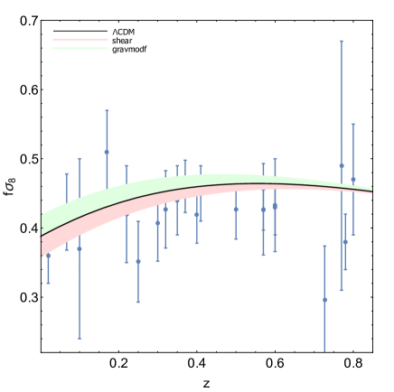
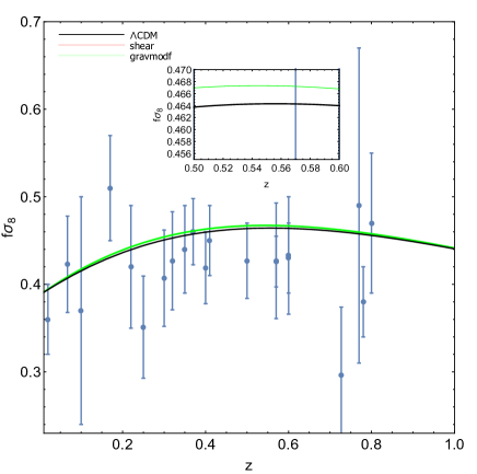
Figure 1: The $f\sigma_{8}$ observable as a function of the redshift. (a) For the shear viscous model the light-red area corresponds to the range of the viscous parameter $0\leq\tilde{\eta}_{0}\leq 2.593\times 10^{-6}$. The green region shows the behavior of modified gravity model with the $\mu_{1}$ parameterization with the range $0\leq E_{1}\leq 0.225$. (b) Plot of the difference between top green line and bottom red line from (a). At $z=0.54$ we have the largest difference between shear and the modified gravity model (detail shown in the inset).

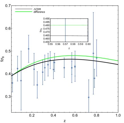
Figure 2: The $f\sigma_{8}$ observable as a function of the redshift. (a) For the shear viscous model the red lines correspond to the range of the viscous parameter $0\leq\tilde{\eta}_{0}\leq 2.593\times 10^{-6}$. Green lines shown the behavior of modified gravity models with the $\mu_{2}$ parameterization. Different values for $E_{2}$ parameter $1.1\leq E_{2}\leq 1.23$ and $1\leq k_{c}\leq 1.1$. (b) Plot of the difference between top green line and bottom red line, from (a). At $z=0.58$ we have the biggest difference between shear and the modified gravity model (detail shown in the inset).

From the three forms of parameterizations, given by Eqs. (22), (23) and (24), respectively, we apply them to Eq. (20). The resulting equation for each case can then be solved numerically for the density contrast $\Delta$. Having also the result for the density contrast from the shear viscous case and obtained from Eq. (11), we can calculate the growth function $f(z)$ for all these different cases. The growth function $f(z)$ is defined as

$$f(z)\equiv\frac{d\ln\frac{\Delta(a)}{\Delta(a_{0})}}{d\ln a}=-(1+z)\frac{d\ln\frac{\Delta(z)}{\Delta(z_{0})}}{dz},$$ (25)

with $z=1/a-1$ and

$$\sigma_{8}(z)=\sigma_{8}(z_{0})\frac{\Delta(z)}{\Delta(z_{0})},$$ (26)

is the redshift-dependent root-mean-square mass fluctuation in spheres with radius $8h^{-1}$ Mpc. The today’s scale factor is set to unity, $a_{0}=1$, thus, $z_{0}=0$. The today’s value adopted here for the variance of the density field at $z_{0}$ is $\sigma_{8}(z_{0})=0.8$, which is consistent with current observations.

Let us consider the results obtained by using the first parametrization given by Eq. (22). In Fig. 1a we show the $f\sigma_{8}$ observable as a function of the redshift. The light-red filled area corresponds to the shear viscous model. This region is set by using our previous results from Ref. Barbosa:2017ojt and corresponds to the range of the viscosity parameter $0\leq\tilde{\eta}\leq 2.593\times 10^{-6}$ at $2\sigma$ of statistical confidence level obtained in that reference. Here, for convenience, we recall we have defined the dimensionless viscous parameter $\tilde{\eta}=24\pi G\eta/H_{0}$ and $\eta$ is assumed to be a constant value, as we have already explained in Sec. II. The viscous shear model equals the $\Lambda$CDM (black line) curve for the case of vanishing viscosity, $\tilde{\eta}=0$. The viscosity parameter, being physically a transport coefficient, should assume only positive values. Thus, its effect acts smoothing the matter clustering in comparison to the standard cosmology, which corresponds to the region below the black line. The value $\tilde{\eta}=2.593\times 10^{-6}$ is the maximum viscosity allowed by the available 21 data points shown in this figure at $2\sigma$ of statistical confidence level (see Ref. Barbosa:2017ojt for details). The shear model with $\tilde{\eta}=2.593\times 10^{-6}$ is the lowest light-red line plotted in Fig. 1a. The green filled area corresponds to modified gravity models based on $\mu_{1}$ and defined in Eq.  (22). Since we expect the values for $\mu_{1}$ to be such that they increase the intensity of gravity Ade:2015rim , then $\mu_{1}$ only assumes positive values. The consequence of this imposition can be seen in Fig. 1a. The green lines always stay above the $\Lambda$CDM line, while the red lines, corresponding to the shear viscosity effect, always stay below the $\Lambda$CDM line.

It is worth noting that both models share the same asymptotic behavior for high redshifts. In particular, the value $E_{1}=0$ corresponds to the $\Lambda$CDM model. Having the bound on $\tilde{\eta}_{0}$ given above in mind, we have plotted the green region in Fig. 1a according to the following criteria: We limit the maximum $f\sigma_{8}(a=1)$ given by the modified gravity model to yield the same departure in magnitude from the $\Lambda$CDM model, but in the opposite direction, in comparison to the shear model. Then, if combining both effects they approximately compensate the effect of each other both today and in the asymptotic past at high redshifts. The combination of both effects is seen in Fig. 1b. Although very tiny, the region around $z=0.54$ is where one finds the largest difference between both effects (inset plot).

In Fig. 2 we present the results obtained by using the second parameterization for the modified gravity effects and given by Eq. (23). The color scheme follows the same as the one used in Fig. 1. We notice from Fig. 2a that now the modified gravity results spread at an uniform distance above the $\Lambda$CDM result for a given value of the constant $E_{2}$. In particular, at low redshifts we again observe a compensation of the modified gravity effect by the shear viscous (or vice-versa), as is apparent from Fig. 2b, where we plot the difference between the maximum differences for each case with respect to the $\Lambda$CDM result. However, at high redshifts the difference starts to get more and more appreciable.

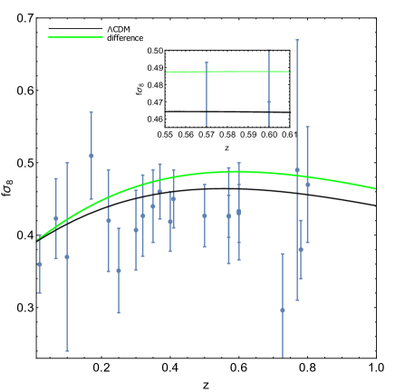
Figure 3: The $f\sigma_{8}$ observable as a function of the redshift. (a) For the shear viscous model the blue lines correspond to the range of the viscous parameter $0\leq\tilde{\eta}_{0}\leq 2.593\times 10^{-6}$. Green lines shown the behavior of modified gravity models with the $\mu_{3}$ parameterization. Different values for $E_{3}$ parameter $0\leq E_{3}\leq 0.13$. (b) Plot of the difference between top green line and bottom red line, from (a). At $z=0.59$ we have the biggest difference between shear and the modified gravity model (detail shown in the inset).

Finally, in Fig. 3 we present the results obtained when considering the parameterization given by Eq. (24). Once again, the color scheme used in Fig. 3a follows the same as the one already used in the previous two figures. The trend observed is similar to the one obtained from the parameterization given by Eq. (23), where we have a tendency of shear viscous effects maskering the modified gravity one and vice-versa at low redshifts, but the difference increases more appreciably at high redshifts, as seen in Fig. 3b.

V On the effects of baryons, bulk viscosity and other possible contributions

We have analysed so far the direct relation between shear viscosity and the slip parameter via the effects on the growth of matter scalar perturbations. This means we have ignored other possible hydrodynamical effects like the presence of a kinetic pressure and bulk viscosity and also the inclusion of a separated baryonic component. Now, our aim in this section is to include such effects in our discussion in order to set a rough estimation on the validity of our approach and showing how they also impact the matter clustering. This analysis shows therefore other degeneracy sources.

Since we have used shear viscosity in this work it is important to mention other dissipative properties. For example, bulk viscosity yields to an additional pressure at the background level. In a FLRW background, with expansion scalar $3H$, the bulk viscous pressure becomes $\Pi=-3H\xi$ where $\xi$ is the coefficient of bulk viscosity. Then, the total pressure of the fluid becomes $P=P_{k}+\Pi$ where $P_{k}$ is the kinetic pressure. The effective equation of state parameter can be written as

$$w=P/\rho=w_{k}-\tilde{\xi}/3,$$ (27)

where we have defined the dimensionless bulk viscous parameter $\tilde{\xi}=24\pi G\xi/H_{0}$ and the kinetic pressure equation of state parameter $w_{k}=P_{k}/\rho$. As shown in Ref. Barbosa:2017ojt bulk and shear viscosities impact the growth of structures at the same level. Indeed, this happens only due to the perturbative dynamics features since values of order $\mathcal{\tilde{\xi}}\lesssim 10^{-5}$ would not affect the background scaling of the matter component. In practise, for such values of the bulk viscous parameter there is no impact at the background level. Therefore, in case the analysis performed in this work had taken also into account bulk viscosity the matter clustering would be even more suppressed. Since the slip parameter is then only related to the shear viscosity this means that in case both shear and bulk viscosities operate the bound on the slip parameter established before would be affected by a factor $\sim 2$. In order to demonstrate this results we present Fig. 4 from Ref. Barbosa:2017ojt . In the first panel of Fig. 4, we have only the effect of the shear viscosity, but no bulk viscosity. This is the same situation as previously shown in this work. In the second panel we show only the effect of the bulk viscosity.

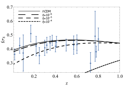
(a) Results when the bulk viscosity is absent.

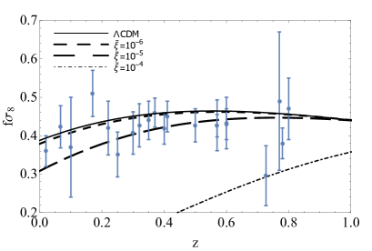
(b) Results when the shear viscosity is absent.

Figure 4: The linear growth against the $f\sigma_{8}$ data as a function of the redshift in the absence and presence of the viscosities.

Now, concerning the possible impact of an extra baryonic component we also take advantage here of the discussion previously presented in Ref. Barbosa:2017ojt . It turns out that an extra baryonic fluid would contribute with a energy density $\rho_{b}$. Its corresponding perturbation $\Delta_{b}$ would act as a source term to the right hand side of Eq. (6). Also, there exist in this case separated conservation equations for the baryonic perturbations similarly to Eqs. (15) and (16).

Let us now present equations in which we can compute both the evolution (obtained already in Barbosa:2017ojt ) of the perturbations of the viscous dark matter fluid (possessing both bulk and shear viscosities) as well as the perturbations of baryons. They are written according to

$$a^{2}\frac{d^{2}\Delta_{b}}{da^{2}}+\Big{\{}3-\frac{3}{2}\frac{H_{0}^{2}}{H^{2}}\left[\Omega_{v}(1+\omega_{v})+\frac{\Omega_{b0}}{a^{3}}\right]\Big{\}}a-\frac{d\Delta_{b}}{da}$$

$$-\frac{3}{2}\frac{H_{0}^{2}}{H^{2}}\frac{\Omega_{b0}}{a^{3}}\Delta_{b}=\Big{[}\frac{3}{2}\frac{H_{0}^{2}}{H^{2}}\Omega_{v}$$

$$+\frac{2\tilde{\eta}a}{3H_{0}\Omega_{v}(1+2\omega_{v})}\Big{(}\frac{3H\omega_{v}}{a}+\frac{H^{2}}{H_{0}^{2}}\frac{\tilde{\xi}\nu}{\Omega_{v}}\left(\frac{\Omega_{v}}{\Omega_{v0}}\right)^{\nu}\Big{)}\Big{]}\Delta_{v}$$

$$-\frac{2\tilde{\eta}Ha}{3H_{0}\Omega_{v}(1+2\omega)}\frac{d\Delta_{v}}{da},$$ (28)

where $\xi=\xi_{0}(\Omega_{v}/\Omega_{v0})^{\nu}$ and $\eta=\eta_{0}(\Omega_{v}/\Omega_{v0})^{\lambda}$.

The viscous fluid density perturbation equation is also modified when including baryons and it now becomes

$$a^{2}\frac{d^{2}\Delta_{v}}{da^{2}}+\left[3-\frac{3}{2}\Omega_{v}\frac{H_{0}^{2}}{H^{2}}-\frac{3}{2}\frac{\Omega_{b0}}{a^{3}}\frac{H_{0}^{2}}{H^{2}}+\bar{A}+k^{2}B\right]a\frac{d\Delta_{v}}{da}$$

$$+\left(\bar{C}+k^{2}D\right)\Delta_{v}=\frac{3}{2}\frac{H_{0}^{2}}{H^{2}}\frac{\Omega_{b0}}{a^{3}}\frac{(1+2\omega_{v})}{(1+\omega_{v})}\Delta_{b},$$ (29)

with $\Delta_{v}\equiv\delta\rho_{v}/(\rho_{v}+\rho_{b})$ and where the factors $\bar{A}$, $B$, $\bar{C}$ and $D$ are defined, respectively, as

$$\bar{A} = A+\frac{3\omega_{v}}{2(1+2\omega_{v})(1+\omega_{v})}\frac{\Omega_{b0}}{a^{3}}\frac{H_{0}^{2}}{H^{2}},$$ (30)

$$B=-\frac{w_{v}(1+\frac{4}{3}R)}{3H^{2}a^{2}(1+w_{v})},$$ (31)

$$\bar{C} = C+\frac{9\omega_{v}(2+6\omega_{v}+5\omega_{v}^{2})}{2(1+2\omega_{v})(1+\omega_{v})}\frac{\Omega_{b0}}{a^{3}}\frac{H_{0}^{2}}{H^{2}}.$$ (32)

and

$$D=\frac{w_{v}^{2}(1+\frac{4}{3}R)}{H^{2}a^{2}(1+w_{v})}(1-\nu)+\frac{\nu\omega_{v}\left(1+2w_{v}\right)}{1+w_{v}}\left(\frac{\Omega_{v}}{\Omega_{v0}}\right)^{\nu}.$$ (33)

The functions $A$ and $B$ have been defined in Barbosa:2017ojt .

In the above equations we have also introduced the quantity $R\equiv\tilde{\eta}/\tilde{\xi}$, i.e., the ratio between the (dimensionless) shear and bulk viscosities which can also be explicitly written as

$$R=\frac{{\tilde{\eta}}_{0}}{{\tilde{\xi}}_{0}}\left(\frac{\Omega_{v}}{\Omega_{v0}}\right)^{\lambda-\nu}.$$ (34)

We have now a two-fluid system described by the coupled equations (28) and (V) and where the baryon density contrast enters as a source term in the dark matter viscous equation one.

It is worth noting that a cosmological observable like $f\sigma_{8}$ takes into account the total matter. This is the case of the standard model in which concerning the linear perturbations both dark matter and baryons are treated as a single matter fluid. There is no distinction between them. Back to the possibility of a separated baryonic fluid let us define then an effective density contrast

$$\Delta_{eff}=\frac{\Omega_{v}\Delta_{v}+\Omega_{b}\Delta_{b}}{\Omega_{v}+\Omega_{b}}$$ (35)

which would be used rather than $\Delta$.

In Fig. 5 we show the evolution of the density contrast considering that both bulk and shear viscosities are present in the cosmic matter with dimensionless viscous parameters $\tilde{\xi}=10^{-5}$ and $\tilde{\eta}=10^{-5}$ (i.e., $R=1$). The dashed-dotted line corresponds to the case in which the entire matter is viscous (i.e., $\Delta_{b}=0$). The solid line corresponds to the case where baryons are accounted for, following Eq. (35). In both cases we notice that the influence of the background expansion is equivalent. This occurs (as already mentioned) because viscosity values of order $\tilde{\xi}\sim 10^{-5}$ do not lead to a relevant deviation from the standard pressureless dark matter background scaling $\rho\sim a^{-3}$. Nevertheless, we note that in the absence of standard pressureless baryons the growth suppression in $\Delta_{eff}$ is not relevant. Therefore, we can conclude that the inclusion of baryons tends to lead to slightly different upper bounds on the dark matter viscosity. If the impact of baryons in the total matter clustering is subdominant we can also conclude that any property assigned to the baryonic sector e.g., viscosities or pressure, should not change the main conclusion of this work which has been based mainly on qualitative grounds.

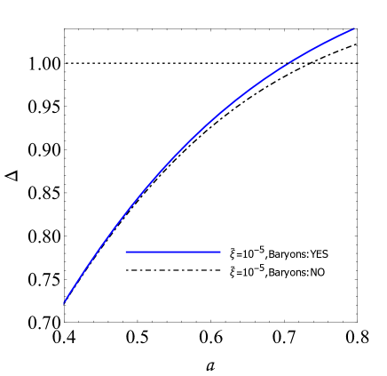
Figure 5: The impact of baryons on the effective density contrast (5.9) as a function of the scale factor.

It is also worth mentioning that the matter fluid could possesses a tiny kinetic pressure. Indeed, the structure formation analysis constrains severely the magnitude of the parameter $w_{k}$ Xu:2013mqe . The equations of the evolution of the matter contrast in the case are slightly different from Eqs. (28) and (V) and are widely know in the literature Xu:2013mqe . For example, Fig. 6 shows the impact of values $w_{k}=\pm 10^{-7}$. From the results shown in Fig. 6, we notice that the kinetic pressure leads to an uniform redshift independent displacement in the $f(z)\sigma_{8}(z)$ evolution. This effect should be contrasted with the one produced, e.g., by the shear viscosity one shown in Fig 3(a), which acts in a more pronounced way at low redshifts. Thus, the effect of the kinetic pressure can, in principle, be distinguished from that of the shear viscosity as more accurate cosmological data become available in the future.

Figure 6: Impact of the kinetic pressure.

VI Conclusions

We have studied in the present work the potential differences in the Newtonian scalar potentials $\Psi$ and $\Phi$ as resulting from both a possible deviation from the GR description for gravity and also by considering that the anisotropic stresses in the energy momentum tensor yield to $\Psi\neq\Phi$. The latter effect due to a shear viscosity that dark matter might be endowed in the GR context. For this study, we have employed three different forms of parameterizing the modified gravity effects through the modification of the Poisson equation for the scalar potential $\Phi$. This is a strategy commonly used in the literature to account the possible modifications generated by different physical scenarios to GR. We have then contrasted these modifications from modified gravity with those from the shear viscous effects when added to GR. To gauge these modifications in the context of the $\Lambda$CDM model, we have made use of the redshift-space-distortion based $f(z)\sigma_{8}(z)$ data, which gives a convenient probe of these different effects at the level of the perturbations.

Our results show that, in general, modified gravity and shear viscosity have opposing effects on the $f(z)\sigma_{8}(z)$ predicted by the $\Lambda$CDM model. While modified gravity tends to enhance the gravitational coupling compared to the GR, thus leading to a stronger matter agglomeration and a larger $f\sigma_{8}$ compared to $\Lambda$CDM, the shear viscosity contribution to GR acts oppositely. This, thus, leads to an interesting possibility of the shear viscosity effects in GR maskering those effects from modified gravity. We have seen that this tends to happen mostly effectively at low redshifts in all three cases of parameterizations of modified gravity that we have considered. This compensation effect is, however, less effective at high redshifts. This points out then for a possible best way for differentiating these effects in future astrophysical searches and probes using high redshift data. In this case, very accurate data on the matter clustering via the $f(z)\sigma_{8}(z)$ measurements might then be able to distinguish the effects studied here.

- (1) B. P. Abbott et al. [LIGO Scientific and Virgo and Fermi-GBM and INTEGRAL Collaborations], “Gravitational Waves and Gamma-rays from a Binary Neutron Star Merger: GW170817 and GRB 170817A,” Astrophys. J. 848, no. 2, L13 (2017) doi:10.3847/2041-8213/aa920c [arXiv:1710.05834 [astro-ph.HE]]. citations counted in INSPIRE as of 13 Jun 2018
- (2) P. Creminelli and F. Vernizzi, “Dark Energy after GW170817 and GRB170817A,” Phys. Rev. Lett. 119, no. 25, 251302 (2017) doi:10.1103/PhysRevLett.119.251302 [arXiv:1710.05877 [astro-ph.CO]].
- (3) J. M. Ezquiaga and M. Zumalacárregui, “Dark Energy After GW170817: Dead Ends and the Road Ahead,” Phys. Rev. Lett. 119, no. 25, 251304 (2017) doi:10.1103/PhysRevLett.119.251304 [arXiv:1710.05901 [astro-ph.CO]].
- (4) P. A. R. Ade et al. [Planck Collaboration], “Planck 2015 results. XIV. Dark energy and modified gravity,” Astron. Astrophys. 594, A14 (2016) doi:10.1051/0004-6361/201525814 [arXiv:1502.01590 [astro-ph.CO]].
- (5) Y. S. Song and W. J. Percival, “Reconstructing the history of structure formation using Redshift Distortions,” JCAP 0910, 004 (2009) doi:10.1088/1475-7516/2009/10/004 [arXiv:0807.0810 [astro-ph]].
- (6) L. Perenon, F. Piazza, C. Marinoni and L. Hui, “Phenomenology of dark energy: general features of large-scale perturbations,” JCAP 1511, no. 11, 029 (2015) doi:10.1088/1475-7516/2015/11/029 [arXiv:1506.03047 [astro-ph.CO]].
- (7) C. M. S. Barbosa, H. Velten, J. C. Fabris and R. O. Ramos, “Assessing the impact of bulk and shear viscosities on large scale structure formation,” Phys. Rev. D 96, no. 2, 023527 (2017) doi:10.1103/PhysRevD.96.023527 [arXiv:1702.07040 [astro-ph.CO]].
- (8) D. B. Thomas, M. Kopp and C. Skordis, “Constraining the Properties of Dark Matter with Observations of the Cosmic Microwave Background,” Astrophys. J. 830, no. 2, 155 (2016)
- (9) M. Kopp, C. Skordis and D. B. Thomas, “Extensive investigation of the generalized dark matter model,” Phys. Rev. D 94, no. 4, 043512 (2016)
- (10) S. Anand, P. Chaubal, A. Mazumdar and S. Mohanty, “Cosmic viscosity as a remedy for tension between PLANCK and LSS data,” JCAP 1711, no. 11, 005 (2017) doi:10.1088/1475-7516/2017/11/005 [arXiv:1708.07030 [astro-ph.CO]].
- (11) M. Bastero-Gil, A. Berera and R. O. Ramos, “Shear viscous effects on the primordial power spectrum from warm inflation,” JCAP 1107, 030 (2011).
- (12) M. Bastero-Gil, A. Berera, I. G. Moss and R. O. Ramos, “Cosmological fluctuations of a random field and radiation fluid,” JCAP 1405, 004 (2014).
- (13) W. Zimdahl, “Bulk viscous cosmology,” Phys. Rev. D 53, 5483 (1996) doi:10.1103/PhysRevD.53.5483 [astro-ph/9601189].
- (14) L. D. Landau and E. M. Lifshitz, Fluid mechanics, Pergamon Press (Oxford, 1975).
- (15) S. Weinberg, Gravitation and Cosmology, (Wiley, New York, 1972).
- (16) L. Amendola, M. Kunz and D. Sapone, “Measuring the dark side (with weak lensing),” JCAP 0804, 013 (2008) doi:10.1088/1475-7516/2008/04/013 [arXiv:0704.2421 [astro-ph]].
- (17) A. De Felice, T. Kobayashi and S. Tsujikawa, “Effective gravitational couplings for cosmological perturbations in the most general scalar-tensor theories with second-order field equations,” Phys. Lett. B 706, 123 (2011) doi:10.1016/j.physletb.2011.11.028 [arXiv:1108.4242 [gr-qc]].
- (18) A. Silvestri, L. Pogosian and R. V. Buniy, “Practical approach to cosmological perturbations in modified gravity,” Phys. Rev. D 87, no. 10, 104015 (2013) doi:10.1103/PhysRevD.87.104015 [arXiv:1302.1193 [astro-ph.CO]].
- (19) J. Zuntz, T. Baker, P. Ferreira and C. Skordis, “Ambiguous Tests of General Relativity on Cosmological Scales,” JCAP 1206, 032 (2012) doi:10.1088/1475-7516/2012/06/032 [arXiv:1110.3830 [astro-ph.CO]].
- (20) D. Clowe, A. Gonzalez and M. Markevitch, “Weak lensing mass reconstruction of the interacting cluster 1E0657-558: Direct evidence for the existence of dark matter,” Astrophys. J. 604, 596 (2004) doi:10.1086/381970 [astro-ph/0312273].
- (21) D. Clowe, M. Bradac, A. H. Gonzalez, M. Markevitch, S. W. Randall, C. Jones and D. Zaritsky, “A direct empirical proof of the existence of dark matter,” Astrophys. J. 648, L109 (2006) doi:10.1086/508162 [astro-ph/0608407].
- (22) G. M. Kremer, M. G. Richarte and F. Teston, “Jeans Instability in a Universe with Dissipation,” Phys. Rev. D 97, no. 2, 023515 (2018) doi:10.1103/PhysRevD.97.023515 [arXiv:1801.06392 [gr-qc]].
- (23) S. Alam, S. Ho and A. Silvestri, “Testing deviations from CDM with growth rate measurements from six large-scale structure surveys at 0.06–1,” Mon. Not. Roy. Astron. Soc. 456, no. 4, 3743 (2016) doi:10.1093/mnras/stv2935 [arXiv:1509.05034 [astro-ph.CO]].
- (24) L. Pogosian, A. Silvestri, K. Koyama and G. B. Zhao, “How to optimally parametrize deviations from General Relativity in the evolution of cosmological perturbations?,” Phys. Rev. D 81, 104023 (2010) doi:10.1103/PhysRevD.81.104023 [arXiv:1002.2382 [astro-ph.CO]].
- (25) R. Bean and M. Tangmatitham, “Current constraints on the cosmic growth history,” Phys. Rev. D 81, 083534 (2010) doi:10.1103/PhysRevD.81.083534 [arXiv:1002.4197 [astro-ph.CO]].
- (26) M. A. Resco and A. L. Maroto, “Parametrizing growth in dark energy and modified gravity models,” Phys. Rev. D 97, no. 4, 043518 (2018) doi:10.1103/PhysRevD.97.043518 [arXiv:1707.08964 [astro-ph.CO]].
- (27) G. R. Dvali, G. Gabadadze and M. Porrati, “4-D gravity on a brane in 5-D Minkowski space,” Phys. Lett. B 485, 208 (2000) doi:10.1016/S0370-2693(00)00669-9 [hep-th/0005016].
- (28) L. Xu and Y. Chang, “Equation of State of Dark Matter after Planck Data,” Phys. Rev. D 88, 127301 (2013) doi:10.1103/PhysRevD.88.127301 [arXiv:1310.1532 [astro-ph.CO]].