An introduction to the SYK model

Vladimir Rosenhaus

Kavli Institute for Theoretical Physics
University of California, Santa Barbara, CA 93106

These notes are a short introduction to the Sachdev-Ye-Kitaev model. We discuss: SYK and tensor models as a new class of large $N$ quantum field theories, the near-conformal invariance in the infrared, the computation of correlation functions, generalizations of SYK, and applications to AdS/CFT and strange metals. In memory of Joe Polchinski

1.  Introduction

The Sachdev-Ye-Kitaev model [1, 2] is a strongly coupled, quantum many-body system that is chaotic, nearly conformally invariant, and exactly solvable. This remarkable and, to date, unique combination of properties have driven the intense activity surrounding SYK and its applications within both high energy and condensed matter physics.

As a quantum field theory, SYK and, more generally, tensor models, constitute a new class of large $N$ theories. The dominance of a simple and well-organized set of Feynman diagrams, iterations of melons, enables the computation of all correlation functions. As a solvable model of holographic duality, SYK accurately captures two-dimensional gravity, and has the potential to shed light on the workings of holography and black holes. As a solvable many-body system, SYK serves as a building block for constructing a metal, capturing some of the properties of non-Fermi liquids.

These notes are a brief introduction to SYK. In Sec. 2 we review large $N$ field theories, in particular vector models, and introduce SYK and tensor models. In Sec. 3 we discuss the low energy limit of SYK, described by a sum of the Schwarzian action and a conformally invariant action. In Sec. 4 we discuss how the simple Feynman diagrammatics of large $N$ SYK, combined with the power of conformal symmetry, allows for an explicit computation of all correlation functions. In Sec. 5 we discuss applications of SYK to holographic duality, and to strange metals.

2.  A New Large $N$ Limit

Large $N$ quantum field theories are theories with a large number of fields, related by some symmetry, such as $O(N)$. Their essential property is the factorization of correlation functions of $O(N)$ invariant operators, $\langle\mathcal{O}(x_{1})\mathcal{O}(x_{2})\rangle=\langle\mathcal{O}(x_{1})\rangle\langle\mathcal{O}(x_{2})\rangle+\frac{1}{N}\left(\ldots\right)$. As such, large $N$ theories are in a sense semi-classical, with $1/N$ playing the role of $\hbar$.

2.1.  Vector models

Figure 1: The self-energy for the $O(N)$ vector model, in terms of the propagator. Iterating gives a sum of bubble diagrams.

The simplest large $N$ quantum field theories are vector models [3, 4]. An example is the $O(N)$ vector model, having $N$ scalar fields, $\vec{\phi}=(\phi^{1},\ldots,\phi^{N})$, with a quartic $O(N)$ invariant interaction,

$$I=\int d^{d}x\left(\frac{1}{2}(\partial\vec{\phi})^{2}+\frac{1}{2}\mu^{2}\vec{\phi}^{\,2}+\frac{g}{4}(\vec{\phi}\cdot\vec{\phi})^{2}\right)~{}.$$ (2.1)

In dimensions $2<d<4$, if one appropriately tunes the bare mass $\mu$, there is an infrared fixed point: the Wilson-Fisher fixed point, describing magnets.

The power of large $N$ is that instead of studying the theory perturbatively in the coupling $g$, one can reorganize the perturbative expansion, into powers of $gN$ and $1/N$. At a given order in $1/N$, one is able to compute to all order in $gN$. For instance, at leading order in $1/N$, the only Feynman diagrams contributing to the two-point function of the $O(N)$ vector model are bubbles, see Fig. 1, all of which are summed by the integral equation,

$$G(p)=\frac{1}{p^{2}+\mu^{2}+\Sigma(p)}~{},\ \ \ \ \Sigma(p)=gN\int d^{d}q\,G(q)~{},$$ (2.2)

where $G(p)$ is the momentum space two-point function, and $\Sigma(p)$ is the self-energy. The self-energy is independent of the momentum: the only effect of the bubble diagrams is to shift the mass. Defining $m^{2}=\mu^{2}+\Sigma$, the above Schwinger-Dyson equation becomes,

$$m^{2}=\mu^{2}+gN\int d^{d}q\frac{1}{q^{2}+m^{2}}~{}.$$ (2.3)

An equivalent way of analyzing the $O(N)$ vector model is by introducing an auxiliary Hubbard-Stratonovich field $\sigma$, so as to rewrite the action as,

$$I=\int d^{d}x\left(\frac{1}{2}(\partial\vec{\phi})^{2}+\frac{1}{2}\mu^{2}\vec{\phi}^{\,2}+\frac{1}{2}\sigma\vec{\phi}^{\,2}-\frac{\sigma^{2}}{4g}\right)~{}.$$ (2.4)

Integrating out $\sigma$ gives back the original action. Alternatively, integrating out the $\phi^{a}$ fields, gives an action involving only $\sigma$,

$$\frac{I_{\sigma}}{N}=\frac{1}{2}\log\det(-\partial^{2}+\mu^{2}+\sigma)-\frac{1}{4gN}\int d^{d}x\,\sigma^{2}~{}.$$ (2.5)

The saddle of $I_{\sigma}$ gives back the Schwinger-Dyson equation for summing bubbles. More generally, one could have introduced a source for $\phi$, and then used the resulting $I_{\sigma}$ to, in principle, compute any correlation function of $O(N)$ invariant operators, to any order in $1/N$.

Matrix Models

There are many systems, such as Yang-Mills theory, in which the fundamental fields are matrices, rather than vectors.  The large $N$ dominant Feynman diagrams in such theories are planar, when drawn in double line notation [10]. There is no known way of summing all planar diagrams, and matrix models are in general not solvable. For some special theories, there are alternate techniques. For instance, models of a single matrix in zero and one dimension can be solved through a map to free fermions [11, 12]. More recently, powerful integrability techniques have been applied to planar $\mathcal{N}=4$ super Yang-Mills in four dimensions[13], yielding, for instance, exact results for anomalous dimensions [14] and progress for the three-point function [15]. See [16] for an introduction to integrability, in two dimensions, and [17] for the initial discovery of the link between the computation of anomalous dimensions and the diagonalization, via Bethe ansatz, of certain integrable spin chain Hamiltonians.

2.2.  Tensor models and SYK

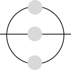
Figure 2: The self-energy for SYK and tensor models, in terms of the propagator. Iterating gives a sum of melon diagrams.

Having discussed vector models and matrix models, it is natural to consider tensor models, with fields having three or more indices. An example of such a model, for fermions in one dimension and rank-3 tensors, is the Klebanov-Tarnopolsky model [18], a simplification of the Gurau-Witten model [19, 20] (see also [21, 22, 23, 24]), with the Lagrangian,

$$L=\frac{1}{2}\sum_{a,b,c=1}^{N}\psi_{abc}\partial_{\tau}\psi_{abc}-\frac{g}{4}\sum_{a_{1},\ldots,c_{2}=1}^{N}\psi_{a_{1}b_{1}c_{1}}\psi_{a_{1}b_{2}c_{2}}\psi_{a_{2}b_{1}c_{2}}\psi_{a_{2}b_{2}c_{1}}~{},$$ (2.6)

where the real field $\psi_{abc}$ transforms in the tri-fundamental representation of $O(N)^{3}$. Remarkably, the two-point function is dominated by melon diagrams in the limit of large $N$ and fixed $J^{2}\equiv g^{2}N^{3}$. The summation of all melon diagrams is encoded in the Schwinger-Dyson equation, see Fig. 2,

$$G(\omega)^{-1}=-i\omega-\Sigma(\omega)~{},\ \ \ \ \ \Sigma(\tau)=J^{2}G(\tau)^{3}~{},$$ (2.7)

where $G(\omega)$ is the Fourier transform of $G(\tau)$. Tensor models, which sum melon diagrams, are more rich, and more difficult, than vector models. They are however, at least in some ways, simpler than matrix models, for which there is no closed set of equations to sum the planar diagrams.

One challenge in the study of tensor models, beyond the melonic dominance at large $N$, is the relatively low degree of symmetry: the number of degrees of freedom scales as $N^{3}$, while the rank of the symmetry group, $O(N)^{3}$, scales as $N^{2}$. This difficulty is alleviated by the SYK model [2], at the expense of introducing disorder,

$$L=\frac{1}{2}\sum_{i=1}^{N}\chi_{i}\partial_{\tau}\chi_{i}-\frac{1}{4!}\sum_{i,j,k,l=1}^{N}J_{ijkl}\chi_{i}\chi_{j}\chi_{k}\chi_{l}~{},$$ (2.8)

where the couplings are Gaussian-random, with zero mean, and variance $\langle J_{ijkl}J_{ijkl}\rangle=6J^{2}/N^{3}$. The leading large $N$ diagrams in SYK are melons; identical to those in the tensor model.  The subleading $1/N$ corrections, as well as the symmetry group, are however different. Taking the partition function, and disorder averaging/integrating out the $J_{ijkl}$ gives a bilocal, $O(N)$ invariant action.  Introducing bilocal fields $\Sigma(\tau_{1},\tau_{2})$ and $G(\tau_{1},\tau_{2})$, with $\Sigma$ acting as a Lagrange multiplier field enforcing $G(\tau_{1},\tau_{2})=\frac{1}{N}\sum_{i=1}^{N}\chi_{i}(\tau_{1})\chi_{i}(\tau_{2})$, and integrating out the fermions, one is left with an action for $\Sigma$ and $G$ [2], see also [27, 28, 29],

$$\frac{I_{eff}}{N}=-\frac{1}{2}\log\det\left(\partial_{\tau}-\Sigma\right)+\frac{1}{2}\int d\tau_{1}d\tau_{2}\left(\Sigma(\tau_{1},\tau_{2})G(\tau_{1},\tau_{2})-\frac{J^{2}}{4}G(\tau_{1},\tau_{2})^{4}\right)~{}.$$ (2.9)

Compared with the $O(N)$ vector model, which was captured by an action for a local field $\sigma(x)$, SYK is instead captured by the above action for bilocal fields $\Sigma(\tau_{1},\tau_{2})$ and $G(\tau_{1},\tau_{2})$.  With this action, the model is in principle solved: instead of the original $N$ fields, there are now only two fields. At infinite $N$, the theory is classical, with the path integral dominated by the saddle for $\Sigma$ and $G$, given by (2.7), reflecting the summation of melon diagrams. All higher point correlation functions follow from expanding the action in powers of $1/N$. The rest of the notes are devoted to computing these in an explicit form, and understanding their physical consequences.

3.  The Infrared

In this section we study SYK in the infrared limit, following [29]. We take the effective action (2.9), and for convenience define, $\sigma(\tau_{1},\tau_{2})=\delta(\tau_{1}-\tau_{2})\partial_{\tau}$, and change variables $\Sigma\rightarrow\Sigma+\sigma$, so that the action becomes, $I_{eff}=I_{CFT}+I_{S}$, where,

$$\frac{I_{CFT}}{N} = -\frac{1}{2}\log\det(-\Sigma)+\frac{1}{2}\int d\tau_{1}d\tau_{2}\left(\Sigma(\tau_{1},\tau_{2})G(\tau_{1},\tau_{2})-\frac{J^{2}}{4}G(\tau_{1},\tau_{2})^{4}\right)$$ (3.1)

$$\frac{I_{S}}{N} = \frac{1}{2}\int d\tau_{1}d\tau_{2}\,\sigma(\tau_{1},\tau_{2})G(\tau_{1},\tau_{2})~{}.$$ (3.2)

In the infrared, $|J\tau|\gg 1$, at leading order, we simply drop the $I_{S}$ part of the action, as the delta function in $\sigma$ is a very UV term. The saddle of $I_{CFT}$ is the Schwinger-Dyson equation from before, without the $\partial_{\tau}$ term, and its solution takes the form of a conformal field theory two-point function [1],

$$G(\tau_{1},\tau_{2})=b\frac{\text{sgn}(\tau_{12})}{|J\tau_{12}|^{2\Delta}}~{},\ \ \ \text{where}\ \ \ b^{4}=\frac{1}{4\pi},\ \ \ \ \Delta=\frac{1}{4},\ \ \ \ \tau_{ij}\equiv\tau_{i}-\tau_{j}~{}.$$ (3.3)

One might assume that any higher point correlation function, computed using $I_{CFT}$, would also be conformally invariant. In fact, this is almost true, but not completely. Notice that $I_{CFT}$ is time reparametrization invariant, $\tau\rightarrow f(\tau)$, provided $G$ and $\Sigma$ transform appropriately,

$$G(\tau_{1},\tau_{2})\rightarrow f^{\prime}(\tau_{1})^{\Delta}f^{\prime}(\tau_{2})^{\Delta}G(f(\tau_{1}),f(\tau_{2}))~{},\ \ \ \ \ \Sigma(\tau_{1},\tau_{2})\rightarrow f^{\prime}(\tau_{1})^{1-\Delta}f^{\prime}(\tau_{2})^{1-\Delta}\Sigma(f(\tau_{1}),f(\tau_{2}))~{}.$$

As a result, in addition to the solution (3.3), we have an entire space of solutions [2],

$$G(\tau_{1},\tau_{2})=b\,\frac{\text{sgn}(\tau_{12})}{J^{2\Delta}}\frac{f^{\prime}(\tau_{1})^{\Delta}f^{\prime}(\tau_{2})^{\Delta}}{|f(\tau_{1})-f(\tau_{2})|^{2\Delta}}~{},$$ (3.4)

and moving between them has no action cost. At a practical level, this means that using $I_{CFT}$ to compute correlation function will lead to divergences [2, 31, 27]. Of course, in the full action, with $I_{S}$ included, there is a cost for $\tau\rightarrow f(\tau)$, so this simply means that we need to move slightly away from the deep infrared limit: rather than just dropping $I_{S}$, we should view it as a perturbation of the infrared action, and compute its effect, to leading order. We approximate $I_{S}$ by inserting for $G$ the saddle (3.4). Since $\sigma(\tau_{1},\tau_{2})$ is a delta function, the integral in the action picks out the $\tau_{12}\ll 1$ part of $G$. Taylor expanding $G(\tau_{1},\tau_{2})$ about $\tau_{+}=(\tau_{1}+\tau_{2})/2$, for $\tau_{12}\ll 1$,

$$G\rightarrow b\frac{\text{sgn}(\tau_{12})}{|J\tau_{12}|^{2\Delta}}\left(1+\frac{\Delta}{6}\tau_{12}^{2}\,\text{Sch}(f(\tau_{+}),\tau_{+})+\ldots\right)~{},\ \ \ \ \text{where }\ \ \ \text{Sch}(f(\tau),\tau)=\frac{f^{\prime\prime\prime}}{f^{\prime}}-\frac{3}{2}\left(\frac{f^{\prime\prime}}{f^{\prime}}\right)^{2}$$

and we get that,

$$\frac{I_{S}}{N}=\frac{\#}{J}\int d\tau\,\text{Sch}(f(\tau),\tau)+\ldots$$ (3.5)

where $\text{Sch}(f(\tau),\tau)$ is the Schwarzian. The prefactor can not be fixed by this procedure; it must be determined numerically [27, 29], from the exact solution to the Schwinger-Dyson equation (2.7). The reason is that we are studying the infrared action, valid for $|J\tau|\gg 1$, while the perturbation $\sigma$ involves a delta function of time, outside the domain of validity of perturbation theory.

The field $f(\tau)$ is sometimes referred to as the reparametrization mode, or the soft mode, or the $h=2$ mode, or the gravitational mode.  It is the Nambu-Goldstone mode for the breaking of time reparametrization invariance [32]. For further studies of the Schwarzian, see [33, 34, 35, 36, 37, 38, 39, 40], as well as references in Sec. 5.1, regarding dilaton gravity.

4.  Correlation Functions

We now turn to higher point correlation functions, following the discussion in [41]. The four-point function, like the two-point function, is given by the solution of an integral equation, while even higher point functions are given by integrals of products of four-point functions. In the infrared, where there is near-conformal symmetry, we can go further and write explicit expressions for the higher point correlation functions. 

4.1.  Conformal blocks

We first recall the constraints that conformal symmetry places on the form of correlation functions. A one-dimensional conformal field theory, CFT₁, has $SL_{2}(R)$ symmetry,

$$\tau\rightarrow\frac{a\tau+b}{c\tau+d}~{},\ \ \ \ ad-bc=1~{}.$$ (4.1)

Any such transformation is generated by a combination of translations $\tau\rightarrow\tau+a$, dilatations $\tau\rightarrow\lambda\tau$, and inversions $\tau\rightarrow\frac{1}{\tau}$. The symmetry fully fixes the functional form of the two-point and three-point functions,

$$\langle\mathcal{O}_{h}(\tau_{1})\mathcal{O}_{h}(\tau_{2})\rangle=\frac{1}{|\tau_{12}|^{2h}}~{},\ \ \ \ \ \ \ \ \ \langle\mathcal{O}_{1}\mathcal{O}_{2}\mathcal{O}_{3}\rangle=\frac{C_{h_{1}h_{2}h_{3}}}{|\tau_{12}|^{h_{1}+h_{2}-h_{3}}|\tau_{13}|^{h_{1}+h_{3}-h_{2}}|\tau_{23}|^{h_{2}+h_{3}-h_{1}}}~{},$$ (4.2)

where the $\mathcal{O}_{i}$, shorthand for $\mathcal{O}_{h_{i}}(\tau_{i})$, are primary operators of dimension $h_{i}$, and the $C_{h_{1}h_{2}h_{3}}$ are structure constants.

To find the functional form of a four-point function, we combine two three-point functions, and integrate over one of the points,

$$\int d\tau_{0}\,\langle\mathcal{O}_{1}\mathcal{O}_{2}\mathcal{O}_{h}(\tau_{0})\rangle\langle\mathcal{O}_{1-h}(\tau_{0})\mathcal{O}_{3}\mathcal{O}_{4}\rangle=\beta(h,h_{34})\mathcal{F}_{1234}^{h}(\tau_{i})+\beta(1-h,h_{12})\mathcal{F}_{1234}^{1-h}(\tau_{i})~{},$$ (4.3)

forming a conformal partial wave, which captures the exchange of $\mathcal{O}_{h}$ and its descendants.  Explicitly evaluating the integral yields the right-hand side: $\beta(h,h_{34})$ is a ratio of gamma functions, whose explicit form we have not written, and $\mathcal{F}_{1234}^{h}(\tau_{i})$ is identified as the conformal block, and contains a hypergeometric function of the conformally invariant cross ratio of the four times $\tau_{1},\ldots,\tau_{4}$, and depends on the dimensions of the external operators, $h_{1},\ldots h_{4}$, and the dimension $h$ of the exchanged operator. The conformal blocks form a basis, in terms of which one can express a general four-point function,

$$\langle\mathcal{O}_{1}\cdots\mathcal{O}_{4}\rangle=\int_{\mathcal{C}}\frac{dh}{2\pi i}\,\rho(h)\mathcal{F}_{1234}^{h}(\tau_{i})~{}.$$ (4.4)

The contour $\mathcal{C}$ runs parallel to the imaginary axis, $h=\frac{1}{2}+is$, and in addition has counterclockwise circles enclosing the positive even integers $h=2n$. These are the principal and discrete series, respectively, of $SL_{2}(R)$. 

As an analogy, this expression for the four-point function is for the conformal group $SL_{2}(R)$ what the Fourier transform is for the translation group. Specifically, we may write any function of $x$ as,

$$f(x)=\int\frac{dp}{2\pi}\,f(p)e^{ipx}~{}.$$ (4.5)

Here $e^{ipx}$ are a complete set of eigenfunctions of the Casimir of the translation group, $\partial_{x}^{2}$, while in (4.4), the conformal blocks $\mathcal{F}_{1234}^{h}(\tau_{i})$, with $h$ running over $\mathcal{C}$, are a complete set of eigenfunctions of the $SL_{2}(R)$ Casimir. Any CFT₁ four-point function is completely specified by an analytic function $\rho(h)$. The poles and residues of $\rho(h)$ set the dimensions and OPE coefficients of the exchanged operators in the four-point function, as one can see by closing the contour in (4.4).

For theories with $O(N)$ symmetry, it is natural to study operators that have definite transformation under the action of $O(N)$. We will be interested in $O(N)$ singlets, such as, 

$$\mathcal{O}_{h}=\frac{1}{N}\sum_{i=1}^{N}\chi_{i}\partial_{\tau}^{1+2n}\chi_{i}~{}.$$ (4.6)

We will refer to such an operator as single-trace. One can make more $O(N)$ invariant operators, by taking products. For instance, a double-trace operator is schematically of the form $\mathcal{O}_{h_{1}}\partial_{\tau}^{2n}\mathcal{O}_{h_{2}}$.

4.2.  SYK correlation functions

We discussed that the fermion two-point function is dominated by melons at large $N$. Now let us look at the Feynman diagrams contributing to a connected fermion $2k$-point function. At leading order, these correlators will scale as $N^{-(k-1)}$, and will involve each external index occurring in pairs. Connecting two such lines by a propagator gives a Feynman diagram contributing to a $2(k\!-\!1)$-point function. Therefore, the Feynman diagrams for a $2k$-point function are found by successively cutting melon diagrams.

(a)

(b)

Figure 3: (a) The four-point function is a sum of ladder diagrams. (b) The kernel that adds rungs to the ladder. Each line denotes the full propagator, so it is actually dressed by melons.

A single cut gives the four-point function: it scales as $1/N$, and is a sum of ladder diagrams, shown in Fig. 3(a), with the kernel, shown in Fig. 3(b), adding rungs to the ladder. To perform the sum, one need only find the eigenfunctions and eigenvalues of the kernel. In fact, as a result of $SL_{2}(R)$ invariance, the eigenfunctions are just the conformal partial waves discussed earlier, labeled by the dimension $h$ of the exchanged operator. In this basis, the sum becomes a geometric sum, and the fermion four-point function is of the form given in (4.4), with $\rho(h)$ [27],

$$\rho(h)=\mu(h)\frac{\alpha_{0}}{2}\frac{k(h)}{1-k(h)}~{},\ \ \ \ \ \ \ \ k(h)=-\frac{3}{2}\frac{\tan\frac{\pi(h-1/2)}{2}}{h-\frac{1}{2}}~{},$$ (4.7)

where $k(h)$ are the eigenvalues of the kernel, while $\mu(h)$ is a simple measure factor and $\alpha_{0}$ is a constant, which we have not written explicitly.  As mentioned earlier, the poles and residues of $\rho(h)$ give the dimensions and OPE coefficients, $c_{h}$, of the exchanged operators. The poles occur at the $h$ for which $k(h)=1$.  These can be written in the form, $h=2n+1+2\Delta+2\epsilon_{n}$, with $\epsilon_{n}$ small for large integer $n$, and correspond to the dimensions of the single-trace operators (4.6) (in the infrared). 

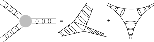
(a)

(b)

Figure 4: (a) The fermion six-point function. (b) A contribution to the eight-point function.

The fermion six-point function consists of the diagrams shown in Fig. 4(a), and can be viewed as three four-point functions glued together. Since the four-point function is expressed in terms of conformal blocks, computing the six-point function is just a matter of gluing together three conformal blocks. The information in the fermion six-point function can be compactly encoded in the three-point functions of the bilinear operators $\mathcal{O}_{h}$ (4.6), with coefficients $C_{h_{1}h_{2}h_{3}}$, whose explicit form is given in [41]: they can be written as $C_{h_{1}h_{2}h_{3}}=c_{h_{1}}c_{h_{2}}c_{h_{3}}\mathcal{I}_{h_{1}h_{2}h_{3}}$, where $\mathcal{I}_{h_{1}h_{2}h_{3}}$ is an analytic function of the $h_{i}$, involving gamma functions and the hypergeometric function ${}_{4}F_{3}$ at argument one.

The fermion eight-point function is built out of more four-point functions glued together. One such contribution is shown in Fig. 4(b), and its contribution to the bilinear four-point function takes an incredibly simple form [41],

$$c_{h_{1}}c_{h_{2}}c_{h_{3}}c_{h_{4}}\int_{\mathcal{C}}\frac{dh}{2\pi i}\,\rho(h)\,\mathcal{I}_{h_{1}h_{2}\,h}\,\mathcal{I}_{h\,h_{3}h_{4}}\,\mathcal{F}_{1234}^{h}(\tau_{i})~{}.$$ (4.8)

The result is intuitive: the $\mathcal{I}_{h_{1}h_{2}\,h}$ and $\mathcal{I}_{h\,h_{3}h_{4}}$ are the “interaction vertices” from the two six-point functions, and there is an operator of dimension $h$ exchanged, giving the $\rho(h)$ factor from the intermediate fermion four-point function. A nontrivial consistency check is that the four-point function of $\mathcal{O}_{h_{i}}$, at order $1/N$, should be a sum of conformal blocks of exchanged single-trace operators as well as double-trace operators. Upon closing the contour in (4.8), the poles of $\rho(h)$ give the single-trace blocks, while the poles of $\mathcal{I}_{h_{1}h_{2}h}$, occurring at $h=h_{1}+h_{2}+2n$, give the double-trace blocks. It is remarkable that the analytically extended OPE coefficients of the single-trace operators - the $\mathcal{I}_{h_{1}h_{2}h_{3}}$ - knew that they should have singularities at precisely these locations.

While SYK has a special set of Feynman diagrams, these results for the correlation functions are more general. The simple expression for the fermion four-point function follows from summing ladder diagrams; it is irrelevant that the propagators are built from melons, those only served to give a conformal two-point function.  The six-point point function is made up of three four-point functions glued together, and in calculating it, it is not relevant that the four-point function was a sum of ladder diagrams. The expression for the eight-point function/bilinear four-point function is valid regardless of the details of how the three fermion four-point functions combine at the “interaction vertex”; all of this is encoded in $\mathcal{I}_{h_{1}h_{2}h_{3}}$.

5.  Applications

5.1.  AdS/CFT

At low energies, SYK is dominated by the $h=2$ mode, described by the Schwarzian action. This is a result of being nearly conformally invariant. On the AdS₂ side, since Einstein gravity is topological in two-dimensions, it is natural to instead consider Jackiw-Teitelboim dilaton gravity [54, 55]. Dilaton gravity theories naturally arise from compactifying gravity in higher dimensions down to two dimensions, with the dilaton playing the role of the size of the extra dimension. It has been shown that the dilaton theory in AdS₂ is the same as the Schwarzian theory, as a consequence of the pattern of symmetry breaking [32, 56, 57]. 

Of course, the $h=2$ mode is just the first in the tower of fermion bilinear $O(N)$ singlets, $\mathcal{O}_{h}$, written schematically in (4.6), and the rest of the tower, with $n\geq 1$, encode the structure of SYK. As we have discussed, a connected $k$-point correlation function of the $\mathcal{O}_{h}$ scales as $N^{-(k-2)/2}$. We can write a putative dual field theory in AdS₂,

$$\mathcal{L}_{bulk}=\sum_{n=1}^{\infty}\frac{1}{2}(\partial\phi_{n})^{2}+\frac{1}{2}m_{n}^{2}\phi_{n}^{2}+\frac{1}{\sqrt{N}}\sum_{n,m,k=1}^{\infty}\lambda_{nmk}\phi_{n}\phi_{m}\phi_{k}+\ldots$$ (5.1)

containing a tower of scalar fields $\phi_{n}$. As a result of the $SL_{2}(R)$ isometry of AdS₂, any correlation function of the $\phi_{n}$, at points extrapolated to the boundary of AdS₂, will take the form of a CFT correlation function. Identifying each $\phi_{n}$ with an operator $\mathcal{O}_{h}$, we can appropriately choose the masses and cubic couplings of the $\phi_{n}$ so as to match to the SYK two-point and three-point functions of the $\mathcal{O}_{h}$, respectively. The masses are related to the dimensions in the standard way, $m_{n}^{2}=h(h-1)$, while the cubic couplings, in the limit $n,m,k\gg 1$ where they simplify, are [41, 68],

$$\lambda_{nmk}\approx\frac{(n+m+k)!}{\Gamma(n+m-k+\frac{1}{2})\Gamma(m+k-n+\frac{1}{2})\Gamma(k+n-m+\frac{1}{2})}~{}.$$ (5.2)

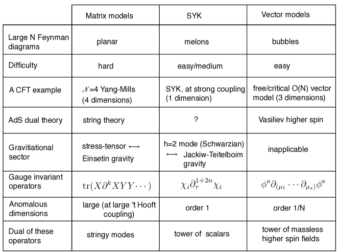
Figure 5: A comparison of SYK to matrix models and vector models. One comment is that for $\mathcal{N}=4$ the anomalous dimensions are large only for the non-supersymmetry protected operators (the half-BPS operators are dual to Kaluza-Klein modes on the $S^{5}$; such operators are ignored in the table). Another, relating to the gravity description, is that it is only at large ’t Hooft coupling, when the stringy modes become very massive, that one can say that the bulk is Einstein gravity. This is to be contrasted with the bulk dual of SYK, where there is no limit in which the tower of bulk fields decouple; their mass is of order-one. Finally, in Vasiliev theory, the spin two field (graviton) is related by symmetry to the other higher spin fields.

One could similarly try to appropriately choose the quartic couplings, so as to match the SYK four-point function of bilinears.  However, in order to have an actual understanding of the AdS dual of SYK, one needs a simple and independently defined bulk theory, something like the string worldsheet action, rather than just a list of couplings. Such a bulk description is presently lacking; it is not obvious one must exist. 

Two canonical examples of AdS/CFT duality are between $\mathcal{N}=4$ super Yang-Mills in 4 dimensions and string theory in AdS${}_{5}\times S^{5}$ [77, 78, 79], and between the free/critical vector $O(N)$ model in 3 dimensions and Vasiliev higher spin theory in AdS₄ [80, 81]. A comparison between SYK and these two theories is given in Table 5.

One hope for SYK has been that, because of its simplicity, it would provide an example of AdS/CFT in which one could fully understand the duality, directly relating the CFT degrees of freedom to the bulk variables. This remains a goal, though achieving it of course requires knowing what the bulk theory is, in order to have a target. Independently of this, SYK has led to a renewed interest in two-dimensional gravity, and the formulation of modern ideas on spacetime and holography in this context, see e.g. [82, 83, 84, 85, 86, 87, 88, 89, 90, 91].

5.2.  Strange metals

There are many variants of SYK, which retain the key feature of dominance of melon diagrams. One natural generalization, which incorporates some of these, is to consider a model which contains $f$ flavors of fermions, with $N_{a}$ fermions of flavor $a$, each appearing $q_{a}$ times in the interaction, so that the Hamiltonian couples $\mathrm{q}=\sum_{a=1}^{f}q_{a}$ fermions together [28],

$$L=\frac{1}{2}\sum_{a=1}^{f}\sum_{i=1}^{N_{a}}\chi_{i}^{a}\,\partial_{\tau}\chi_{i}^{a}+\frac{(i)^{\frac{\mathrm{q}}{2}}}{\prod_{a=1}^{f}q_{a}!}\sum_{I}J_{I}(\chi_{i_{1}}^{1}\cdots\chi_{i_{q_{1}}}^{1})\cdots(\chi_{j_{1}}^{f}\cdots\chi_{j_{q_{f}}}^{f})~{},$$ (5.3)

where $I$ is a collective index, $I=i_{1},\ldots,i_{q_{1}},\ldots,j_{1},\ldots,j_{q_{f}}$. The coupling $J_{I}$ is antisymmetric under permutation of indices within any one of the $f$ families, and is drawn from a Gaussian distribution. This model with one flavor, $f=1$, reduces to the standard SYK model with a $q$-body interaction, sometimes denoted by SYK_q; further setting $q=4$ gives the canonical SYK model, which has been the focus of these notes. 

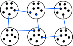
Figure 6: A lattice of SYK “quantum dots”, with quartic all-to-all interactions within a dot, the third term in (5.4), and quadratic hopping terms between dots, the second term in (5.4).

Regarding flavor as a lattice site index, $x$, and taking sums of the flavored models, one can build lattices of SYK models [109]. One such model, having some features of a strongly correlated metal, is [110],

$$L=\sum_{x}\sum_{i}c_{i,x}^{\dagger}\left(\partial_{\tau}-\mu\right)c_{i,x}-\sum_{\langle xx^{\prime}\rangle}\sum_{i,j}t_{ij,xx^{\prime}}c_{i,x}^{\dagger}c_{j,x^{\prime}}-\sum_{x}\sum_{i,j,k,l}J_{ijkl,x}c_{i,x}^{\dagger}c_{j,x}^{\dagger}c_{k,x}c_{l,x}~{}.\vspace{-.2cm}$$ (5.4)

Here $t_{ij,xx^{\prime}}$ and $J_{ijkl,x}$ are again random couplings, and the $c_{i,x}$ are now complex fermions. A cartoon of this model is shown in Fig. 6. The model exhibits incoherent metal behavior, with resistivity scaling linearly with temperature, at high temperature, and Fermi liquid behavior at low temperature. 

More generally, the fact that SYK is a system without quasiparticles, yet is nevertheless solvable, makes it a valuable tool with which to study transport and chaos [117, 118, 119, 120, 121, 122, 123, 124, 125], non-equilibrium dynamics and entanglement [126, 127, 128, 129], and eigenstate thermalization [130, 131, 132]. There are limitations, however, as neither the all-to-all interactions nor the large $N$, which are essential to the solvability of SYK, are present in real metals.

Finally, there are a number of topics which we have not discussed, such as: experimental realizations and quantum simulations of SYK [133, 134, 135, 136, 137, 138, 139], the zero-temperature entropy (an infinite $N$ artifact) [140, 141, 142], studies of the spectral density, the spectral form factor, and connections with random matrix theory [83, 143, 144, 145, 146, 147, 148, 149, 150, 151, 152, 153].

References

- [1] S. Sachdev and J. Ye, “Gapless spin-fluid ground state in a random quantum heisenberg magnet,” Phys. Rev. Lett. 70 (May, 1993) 3339–3342. http://link.aps.org/doi/10.1103/PhysRevLett.70.3339.
- [2] A. Kitaev, “A simple model of quantum holography,” KITP strings seminar and Entanglement 2015 program (Feb. 12, April 7, and May 27, 2015) . http://online.kitp.ucsb.edu/online/entangled15/.
- [3] S. Coleman, Aspects of Symmetry. Cambridge University Press, 1985.
- [4] D. J. Gross and A. Neveu, “Dynamical Symmetry Breaking in Asymptotically Free Field Theories,” Phys. Rev. D10 (1974) 3235.
- [5] N. Iizuka and J. Polchinski, “A Matrix Model for Black Hole Thermalization,” JHEP 10 (2008) 028, arXiv:0801.3657 [hep-th].
- [6] G. ’t Hooft, “A Two-Dimensional Model for Mesons,” Nucl. Phys. B75 (1974) 461–470.
- [7] C. G. Callan, Jr., N. Coote, and D. J. Gross, “Two-Dimensional Yang-Mills Theory: A Model of Quark Confinement,” Phys. Rev. D13 (1976) 1649.
- [8] S. Giombi, S. Minwalla, S. Prakash, S. P. Trivedi, S. R. Wadia, and X. Yin, “Chern-Simons Theory with Vector Fermion Matter,” Eur. Phys. J. C72 (2012) 2112, arXiv:1110.4386 [hep-th].
- [9] O. Aharony, G. Gur-Ari, and R. Yacoby, “d=3 Bosonic Vector Models Coupled to Chern-Simons Gauge Theories,” JHEP 03 (2012) 037, arXiv:1110.4382 [hep-th].
- [10] G. ’t Hooft, “A Planar Diagram Theory for Strong Interactions,” Nucl. Phys. B72 (1974) 461. [,337(1973)].
- [11] P. Di Francesco, P. H. Ginsparg, and J. Zinn-Justin, “2-D Gravity and random matrices,” arXiv:hep-th/9306153
- [12] I. R. Klebanov, “String theory in two-dimensions,” arXiv:hep-th/9108019 [hep-th].
- [13] N. Beisert et al., “Review of AdS/CFT Integrability: An Overview,” arXiv:1012.3982 [hep-th].
- [14] N. Gromov, V. Kazakov, S. Leurent, and D. Volin, “Quantum Spectral Curve for Planar Super-Yang-Mills Theory,” Phys. Rev. Lett. 112 no. 1, (2014) 011602, arXiv:1305.1939 [hep-th].
- [15] B. Basso, S. Komatsu, and P. Vieira, “Structure Constants and Integrable Bootstrap in Planar N=4 SYM Theory,” arXiv:1505.06745 [hep-th].
- [16] A. B. Zamolodchikov and A. B. Zamolodchikov, “Factorized s Matrices in Two-Dimensions as the Exact Solutions of Certain Relativistic Quantum Field Models,” Annals Phys. 120 (1979) 253–291.
- [17] J. A. Minahan and K. Zarembo, “The Bethe ansatz for N=4 superYang-Mills,” JHEP 03 (2003) 013, arXiv:hep-th/0212208 [hep-th].
- [18] I. R. Klebanov and G. Tarnopolsky, “Uncolored random tensors, melon diagrams, and the Sachdev-Ye-Kitaev models,” Phys. Rev. D95 no. 4, (2017) 046004, arXiv:1611.08915 [hep-th].
- [19] R. Gurau, “Colored Group Field Theory,” Commun. Math. Phys. 304 (2011) 69–93, arXiv:0907.2582 [hep-th].
- [20] E. Witten, “An SYK-Like Model Without Disorder,” arXiv:1610.09758 [hep-th].
- [21] V. Bonzom, R. Gurau, A. Riello, and V. Rivasseau, “Critical behavior of colored tensor models in the large N limit,” Nucl. Phys. B853 (2011) 174–195, arXiv:1105.3122 [hep-th].
- [22] S. Carrozza and A. Tanasa, “O( N) Random Tensor Models,” Letters in Mathematical Physics 106 (Nov., 2016) 1531–1559, arXiv:1512.06718 [math-ph].
- [23] N. Delporte and V. Rivasseau, “The Tensor Track V: Holographic Tensors,” arXiv:1804.11101 [hep-th].
- [24] I. R. Klebanov and G. Tarnopolsky, “On Large Limit of Symmetric Traceless Tensor Models,” JHEP 10 (2017) 037, arXiv:1706.00839 [hep-th].
- [25] R. Gurau, “Quenched equals annealed at leading order in the colored SYK model,” EPL 119 no. 3, (2017) 30003, arXiv:1702.04228 [hep-th].
- [26] B. Michel, J. Polchinski, V. Rosenhaus, and S. J. Suh, “Four-point function in the IOP matrix model,” JHEP 05 (2016) 048, arXiv:1602.06422 [hep-th].
- [27] J. Maldacena and D. Stanford, “Comments on the Sachdev-Ye-Kitaev model,” arXiv:1604.07818 [hep-th].
- [28] D. J. Gross and V. Rosenhaus, “A Generalization of Sachdev-Ye-Kitaev,” JHEP 02 (2017) 093, arXiv:1610.01569 [hep-th].
- [29] A. Kitaev and S. J. Suh, “The soft mode in the Sachdev-Ye-Kitaev model and its gravity dual,” arXiv:1711.08467 [hep-th].
- [30] A. Georges, G. Kotliar, W. Krauth, and M. J. Rozenberg, Rev. Mod. Phys. 68 (Jan, 1996) 13–125 ; A. Georges, “Applications of Dynamical Mean Field Theory,” (Aug. 20, 2015) . http://online.kitp.ucsb.edu/online/latticeqcd15/dmft/.
- [31] J. Polchinski and V. Rosenhaus, “The Spectrum in the Sachdev-Ye-Kitaev Model,” JHEP 04 (2016) 001, arXiv:1601.06768 [hep-th].
- [32] J. Maldacena, D. Stanford, and Z. Yang, “Conformal symmetry and its breaking in two dimensional Nearly Anti-de-Sitter space,” arXiv:1606.01857 [hep-th].
- [33] A. Jevicki, K. Suzuki, and J. Yoon, “Bi-Local Holography in the SYK Model,” JHEP 07 (2016) 007, arXiv:1603.06246 [hep-th].; A. Jevicki and K. Suzuki, “Bi-Local Holography in the SYK Model: Perturbations,” JHEP 11 (2016) 046, arXiv:1608.07567 [hep-th].
- [34] D. Bagrets, A. Altland, and A. Kamenev, “Sachdev-Ye-Kitaev model as Liouville quantum mechanics,” Nucl. Phys. B911 (2016) 191–205, arXiv:1607.00694 [cond-mat.str-el]; D. Bagrets, A. Altland, and A. Kamenev, “Power-law out of time order correlation functions in the SYK model,” Nucl. Phys. B921 (2017) 727–752, arXiv:1702.08902 [cond-mat.str-el].
- [35] D. Stanford and E. Witten, “Fermionic Localization of the Schwarzian Theory,” JHEP 10 (2017) 008, arXiv:1703.04612 [hep-th].
- [36] T. G. Mertens, G. J. Turiaci, and H. L. Verlinde, “Solving the Schwarzian via the Conformal Bootstrap,” JHEP 08 (2017) 136, arXiv:1705.08408 [hep-th].
- [37] T. G. Mertens, “The Schwarzian Theory - Origins,” arXiv:1801.09605 [hep-th]; A. Blommaert, T. G. Mertens, and H. Verschelde, “The Schwarzian Theory - A Wilson Line Perspective,” arXiv:1806.07765 [hep-th].
- [38] G. Mandal, P. Nayak, and S. R. Wadia, “Coadjoint orbit action of Virasoro group and two-dimensional quantum gravity dual to SYK/tensor models,” JHEP 11 (2017) 046, arXiv:1702.04266 [hep-th]. A. Gaikwad, L. K. Joshi, G. Mandal, and S. R. Wadia, “Holographic dual to charged SYK from 3D Gravity and Chern-Simons,” arXiv:1802.07746 [hep-th].
- [39] A. Alekseev and S. L. Shatashvili, “Coadjoint Orbits, Cocycles and Gravitational Wess-Zumino,” in Ludwig Faddeev Memorial Volume, pp. 37–51. 2018. arXiv:1801.07963 [hep-th].
- [40] V. V. Belokurov and E. T. Shavgulidze, “Correlation functions in the Schwarzian theory,” arXiv:1804.00424 [hep-th].
- [41] D. J. Gross and V. Rosenhaus, “All point correlation functions in SYK,” JHEP 12 (2017) 148, arXiv:1710.08113 [hep-th].
- [42] D. J. Gross and V. Rosenhaus, “A line of CFTs: from generalized free fields to SYK,” JHEP 07 (2017) 086, arXiv:1706.07015 [hep-th].
- [43] A. Kitaev, “Notes on representations,” arXiv:1711.08169 [hep-th].
- [44] J. Murugan, D. Stanford, and E. Witten, “More on Supersymmetric and 2d Analogs of the SYK Model,” JHEP 08 (2017) 146, arXiv:1706.05362 [hep-th].
- [45] K. Bulycheva, “A note on the SYK model with complex fermions,” JHEP 12 (2017) 069, arXiv:1706.07411 [hep-th].
- [46] V. K. Dobrev, G. Mack, V. B. Petkova, S. G. Petrova, and I. T. Todorov, “Harmonic Analysis on the n-Dimensional Lorentz Group and Its Application to Conformal Quantum Field Theory,” Lect. Notes Phys. 63 (1977) 1–280.
- [47] D. Karateev, P. Kravchuk, and D. Simmons-Duffin, “Weight Shifting Operators and Conformal Blocks,” JHEP 02 (2018) 081, arXiv:1706.07813 [hep-th].; P. Kravchuk and D. Simmons-Duffin, “Light-ray operators in conformal field theory,” arXiv:1805.00098 [hep-th].
- [48] S. Caron-Huot, “Analyticity in Spin in Conformal Theories,” arXiv:1703.00278 [hep-th].; D. Simmons-Duffin, D. Stanford and E. Witten, “A spacetime derivation of the Lorentzian OPE inversion formula,” arXiv:1711.03816 [hep-th].
- [49] T. Raben and C.-I. Tan, “Minkowski Conformal Blocks and the Regge Limit for SYK-like Models,” arXiv:1801.04208 [hep-th].
- [50] A. Gadde, “In search of conformal theories,” arXiv:1702.07362 [hep-th].
- [51] D. Simmons-Duffin, “Projectors, Shadows, and Conformal Blocks,” JHEP 04 (2014) 146, arXiv:1204.3894 [hep-th].
- [52] J. Maldacena, S. H. Shenker, and D. Stanford, “A bound on chaos,” JHEP 08 (2016) 106, arXiv:1503.01409 [hep-th].
- [53] D. Grabner, N. Gromov, V. Kazakov and G. Korchemsky, Phys. Rev. Lett. 120, no. 11, 111601 (2018) arXiv:1711.04786 [hep-th].
- [54] R. Jackiw, “Lower Dimensional Gravity,” Nucl. Phys. B252 (1985) 343–356; C. Teitelboim, “Gravitation and Hamiltonian Structure in Two Space-Time Dimensions,” Phys. Lett. B126 (1983) 41–45.
- [55] A. Almheiri and J. Polchinski, “Models of AdS2 backreaction and holography,” JHEP 11 (2015) 014, arXiv:1402.6334 [hep-th].
- [56] K. Jensen, “Chaos and hydrodynamics near AdS2,” Phys. Rev. Lett. 117 no. 11, (2016) 111601, arXiv:1605.06098 [hep-th].
- [57] J. Engels y, T. G. Mertens, and H. Verlinde, “An investigation of AdS2 backreaction and holography,” JHEP 07 (2016) 139, arXiv:1606.03438 [hep-th].
- [58] S. Dubovsky, V. Gorbenko, and M. Mirbabayi, “Asymptotic fragility, near AdS2 holography and ,” JHEP 09 (2017) 136, arXiv:1706.06604 [hep-th].
- [59] S. Forste and I. Golla, “Nearly AdS2 sugra and the super-Schwarzian,” Phys. Lett. B771 (2017) 157–161, arXiv:1703.10969 [hep-th]; S. Forste, J. Kames-King, and M. Wiesner, “Towards the Holographic Dual of N = 2 SYK,” JHEP 03 (2018) 028, arXiv:1712.07398 [hep-th].
- [60] F. M. Haehl and M. Rozali, “Fine Grained Chaos in Gravity,” arXiv:1712.04963 [hep-th].
- [61] D. Grumiller, R. McNees, J. Salzer, C. Valc rcel, and D. Vassilevich, “Menagerie of AdS2 boundary conditions,” JHEP 10 (2017) 203, arXiv:1708.08471 [hep-th].
- [62] H. A. Gonz lez, D. Grumiller, and J. Salzer, “Towards a bulk description of higher spin SYK,” JHEP 05 (2018) 083, arXiv:1802.01562 [hep-th].
- [63] H. T. Lam, T. G. Mertens, G. J. Turiaci, and H. Verlinde, “Shockwave S-matrix from Schwarzian Quantum Mechanics,” arXiv:1804.09834 [hep-th].
- [64] Y.-H. Qi, Y. Seo, S.-J. Sin, and G. Song, “Schwarzian correction to quantum correlation in SYK model,” arXiv:1804.06164 [hep-th].
- [65] M. Taylor, “Generalized conformal structure, dilaton gravity and SYK,” JHEP 01 (2018) 010, arXiv:1706.07812 [hep-th].
- [66] P. Nayak, A. Shukla, R. M. Soni, S. P. Trivedi, and V. Vishal, “On the Dynamics of Near-Extremal Black Holes,” arXiv:1802.09547 [hep-th].
- [67] Y.-Z. Li, S.-L. Li, and H. Lu, “Exact Embeddings of JT Gravity in Strings and M-theory,” arXiv:1804.09742 [hep-th].; I. Bena, P. Heidmann, and D. Turton, “AdS2 Holography: Mind the Cap,” arXiv:1806.02834 [hep-th].; F. Larsen, “A nAttractor Mechanism for nAdS(2)/nCFT(1) Holography,” arXiv:1806.06330 [hep-th]. K. S. Kolekar and K. Narayan, “ dilaton gravity from reductions of some nonrelativistic theories,” arXiv:1803.06827 [hep-th].
- [68] D. J. Gross and V. Rosenhaus, “The Bulk Dual of SYK: Cubic Couplings,” JHEP 05 (2017) 092, arXiv:1702.08016 [hep-th].
- [69] S. R. Das, A. Ghosh, A. Jevicki, and K. Suzuki, “Three Dimensional View of Arbitrary SYK models,” JHEP 02 (2018) 162, arXiv:1711.09839 [hep-th].
- [70] W. A. Bardeen, I. Bars, A. J. Hanson, and R. D. Peccei, “A Study of the Longitudinal Kink Modes of the String,” Phys. Rev. D13 (1976) 2364–2382.
- [71] D. J. Gross and V. Rosenhaus, in progress .
- [72] K. Bulycheva, I. R. Klebanov, A. Milekhin, and G. Tarnopolsky, “Spectra of Operators in Large Tensor Models,” Phys. Rev. D97 no. 2, (2018) 026016, arXiv:1707.09347 [hep-th].
- [73] S. Choudhury, A. Dey, I. Halder, L. Janagal, S. Minwalla, and R. Poojary, “Notes on Melonic Tensor Models,” arXiv:1707.09352 [hep-th].
- [74] M. Beccaria and A. A. Tseytlin, “Partition function of free conformal fields in 3-plet representation,” JHEP 05 (2017) 053, arXiv:1703.04460 [hep-th].
- [75] H. Itoyama, A. Mironov, and A. Morozov, “Ward identities and combinatorics of rainbow tensor models,” arXiv:1704.08648 [hep-th]. P. Diaz and S.-J. Rey, “Orthogonal Bases of Invariants in Tensor Models,” arXiv:1706.02667 [hep-th].; R. de Mello Koch, R. Mello Koch, D. Gossman, and L. Tribelhorn, “Gauge Invariants, Correlators and Holography in Bosonic and Fermionic Tensor Models,” arXiv:1707.01455 [hep-th].; J. Ben Geloun and S. Ramgoolam, “Tensor Models, Kronecker coefficients and Permutation Centralizer Algebras,” arXiv:1708.03524 [hep-th]; C. Krishnan, K. V. Pavan Kumar, and D. Rosa, “Contrasting SYK-like Models,” arXiv:1709.06498 [hep-th].;
- [76] M. A. Vasiliev, “From Coxeter Higher-Spin Theories to Strings and Tensor Models,” arXiv:1804.06520 [hep-th].
- [77] J. M. Maldacena, “The Large N limit of superconformal field theories and supergravity,” Int. J. Theor. Phys. 38 (1999) 1113–1133, arXiv:hep-th/9711200 [hep-th]. [Adv. Theor. Math. Phys.2,231(1998)].
- [78] S. S. Gubser, I. R. Klebanov, and A. M. Polyakov, “Gauge theory correlators from noncritical string theory,” Phys. Lett. B428 (1998) 105–114, arXiv:hep-th/9802109 [hep-th].
- [79] E. Witten, “Anti-de Sitter space and holography,” Adv. Theor. Math. Phys. 2 (1998) 253–291, arXiv:hep-th/9802150 [hep-th].
- [80] I. R. Klebanov and A. M. Polyakov, “AdS dual of the critical O(N) vector model,” Phys. Lett. B550 (2002) 213–219, arXiv:hep-th/0210114 [hep-th].
- [81] S. Giombi,“TASI Lectures on the Higher Spin - CFT duality,” arXiv:1607.02967 [hep-th].
- [82] H. Ooguri and C. Vafa, “Non-supersymmetric AdS and the Swampland,” arXiv:1610.01533 [hep-th].; B. Freivogel and M. Kleban, “Vacua Morghulis,” arXiv:1610.04564 [hep-th].
- [83] J. S. Cotler, G. Gur-Ari, M. Hanada, J. Polchinski, P. Saad, S. H. Shenker, D. Stanford, A. Streicher, and M. Tezuka, “Black Holes and Random Matrices,” JHEP 05 (2017) 118, arXiv:1611.04650 [hep-th]
- [84] P. Saad, S. H. Shenker, and D. Stanford, “A semiclassical ramp in SYK and in gravity,” arXiv:1806.06840 [hep-th].
- [85] J. Maldacena, D. Stanford, and Z. Yang, “Diving into traversable wormholes,” Fortsch. Phys. 65 no. 5, (2017) 1700034, arXiv:1704.05333 [hep-th].
- [86] I. Kourkoulou and J. Maldacena, “Pure states in the SYK model and nearly- gravity,” arXiv:1707.02325 [hep-th].
- [87] J. Maldacena and X.-L. Qi, “Eternal traversable wormhole,” arXiv:1804.00491 [hep-th].
- [88] A. R. Brown and L. Susskind, “Second law of quantum complexity,” arXiv:1701.01107 [hep-th].
- [89] P. Caputa, N. Kundu, M. Miyaji, T. Takayanagi, and K. Watanabe, “Liouville Action as Path-Integral Complexity: From Continuous Tensor Networks to AdS/CFT,” JHEP 11 (2017) 097, arXiv:1706.07056 [hep-th].
- [90] D. Harlow and D. Jafferis, “The Factorization Problem in Jackiw-Teitelboim Gravity,” arXiv:1804.01081 [hep-th].
- [91] B. Swingle, “Spacetime from entanglement,” Annual Review of Condensed Matter Physics 9 no. 1, (2018) 345–358, https://doi.org/10.1146/annurev-conmatphys-033117-054219.
- [92] W. Fu, D. Gaiotto, J. Maldacena, and S. Sachdev, “Supersymmetric Sachdev-Ye-Kitaev models,” Phys. Rev. D95 no. 2, (2017) 026009, arXiv:1610.08917 [hep-th].
- [93] N. Sannomiya, H. Katsura, and Y. Nakayama, “Supersymmetry breaking and Nambu-Goldstone fermions with cubic dispersion,” Phys. Rev. D95 no. 6, (2017) 065001, arXiv:1612.02285 [cond-mat.str-el].
- [94] C. Peng, M. Spradlin, and A. Volovich, “Correlators in the Supersymmetric SYK Model,” JHEP 10 (2017) 202, arXiv:1706.06078 [hep-th].
- [95] K. Bulycheva, “ SYK model in the superspace formalism,” JHEP 04 (2018) 036, arXiv:1801.09006 [hep-th].
- [96] P. Narayan and J. Yoon, “Supersymmetric SYK Model with Global Symmetry,” arXiv:1712.02647 [hep-th].
- [97] D. Anninos, T. Anous, and F. Denef, “Disordered Quivers and Cold Horizons,” JHEP 12 (2016) 071, arXiv:1603.00453 [hep-th].
- [98] S. Giombi, I. R. Klebanov, and G. Tarnopolsky, “Bosonic tensor models at large and small ,” Phys. Rev. D96 no. 10, (2017) 106014, arXiv:1707.03866 [hep-th].
- [99] S. Prakash and R. Sinha, “A Complex Fermionic Tensor Model in Dimensions,” JHEP 02 (2018) 086, arXiv:1710.09357 [hep-th].
- [100] D. Benedetti, S. Carrozza, R. Gurau, and A. Sfondrini, “Tensorial Gross-Neveu models,” JHEP 01 (2018) 003, arXiv:1710.10253 [hep-th].
- [101] T. Azeyanagi, F. Ferrari, and F. I. Schaposnik Massolo, “Phase Diagram of Planar Matrix Quantum Mechanics, Tensor, and Sachdev-Ye-Kitaev Models,” Phys. Rev. Lett. 120 no. 6, (2018) 061602, arXiv:1707.03431 [hep-th].
- [102] C. Peng, M. Spradlin, and A. Volovich, “A Supersymmetric SYK-like Tensor Model,” JHEP 05 (2017) 062, arXiv:1612.03851 [hep-th].
- [103] C.-M. Chang, S. Colin-Ellerin, and M. Rangamani, “On Melonic Supertensor Models,” arXiv:1806.09903 [hep-th].
- [104] Z. Bi, C.-M. Jian, Y.-Z. You, K. A. Pawlak, and C. Xu, “Instability of the non-Fermi liquid state of the Sachdev-Ye-Kitaev Model,” Phys. Rev. B95 no. 20, (2017) 205105, arXiv:1701.07081 [cond-mat.str-el].
- [105] M. Berkooz, P. Narayan, M. Rozali, and J. Simon, “Higher Dimensional Generalizations of the SYK Model,” JHEP 01 (2017) 138, arXiv:1610.02422 [hep-th]; M. Berkooz, P. Narayan, M. Rozali, and J. Simon, “Comments on the Random Thirring Model,” JHEP 09 (2017) 057, arXiv:1702.05105 [hep-th].
- [106] C. Peng, “ SYK, Chaos and Higher-Spins,” arXiv:1805.09325 [hep-th].
- [107] G. Turiaci and H. Verlinde, “Towards a 2d QFT Analog of the SYK Model,” JHEP 10 (2017) 167, arXiv:1701.00528 [hep-th].
- [108] S. S. Gubser, M. Heydeman, C. Jepsen, S. Parikh, I. Saberi, B. Stoica, and B. Trundy, “Signs of the time: Melonic theories over diverse number systems,” arXiv:1707.01087 [hep-th].
- [109] Y. Gu, X.-L. Qi, and D. Stanford, “Local criticality, diffusion and chaos in generalized Sachdev-Ye-Kitaev models,” JHEP 05 (2017) 125, arXiv:1609.07832.
- [110] X.-Y. Song, C.-M. Jian, and L. Balents, “Strongly Correlated Metal Built from Sachdev-Ye-Kitaev Models,” Phys. Rev. Lett. 119 no. 21, (Nov., 2017) 216601, arXiv:1705.00117 [cond-mat.str-el].
- [111] S. Banerjee and E. Altman, “Solvable model for a dynamical quantum phase transition from fast to slow scrambling,” Phys. Rev. B95 no. 13, (2017) 134302, arXiv:1610.04619 [cond-mat.str-el].
- [112] S.-K. Jian and H. Yao, “Solvable Sachdev-Ye-Kitaev models in higher dimensions: from diffusion to many-body localization,” Phys. Rev. Lett. 119 no. 20, (2017) 206602, arXiv:1703.02051 [cond-mat.str-el].
- [113] D. Chowdhury, Y. Werman, E. Berg, and T. Senthil, “Translationally invariant non-Fermi liquid metals with critical Fermi-surfaces: Solvable models,” arXiv:1801.06178 [cond-mat.str-el].
- [114] W. Fu, Y. Gu, S. Sachdev, and G. Tarnopolsky, “ fractionalized phases of a solvable, disordered, - model,” arXiv:1804.04130 [cond-mat.str-el].
- [115] A. A. Patel, M. J. Lawler and E. A. Kim, “Coherent superconductivity with large gap ratio from incoherent metals,” arXiv:1805.11098 [cond-mat.str-el].
- [116] X. Wu, X. Chen, C.-M. Jian, Y.-Z. You, and C. Xu, “A candidate Theory for the ”Strange Metal” phase at Finite Energy Window,” arXiv:1802.04293 [cond-mat.str-el].
- [117] R. A. Davison, W. Fu, A. Georges, Y. Gu, K. Jensen, and S. Sachdev, “Thermoelectric transport in disordered metals without quasiparticles: The Sachdev-Ye-Kitaev models and holography,” Phys. Rev. B95 no. 15, (2017) 155131, arXiv:1612.00849 [cond-mat.str-el].
- [118] Y. Gu, A. Lucas, and X.-L. Qi, “Energy diffusion and the butterfly effect in inhomogeneous Sachdev-Ye-Kitaev chains,” SciPost Phys. 2 no. 3, (2017) 018, arXiv:1702.08462 [hep-th].
- [119] C. Peng, “Vector models and generalized SYK models,” JHEP 05 (2017) 129, arXiv:1704.04223 [hep-th].
- [120] Y. Chen, H. Zhai, and P. Zhang, “Tunable Quantum Chaos in the Sachdev-Ye-Kitaev Model Coupled to a Thermal Bath,” JHEP 07 (2017) 150, arXiv:1705.09818 [hep-th].
- [121] A. A. Patel, J. McGreevy, D. P. Arovas, and S. Sachdev, “Magnetotransport in a model of a disordered strange metal,” Phys. Rev. X8 no. 2, (2018) 021049, arXiv:1712.05026 [cond-mat.str-el].
- [122] S. Mondal, “Chaos, Instability and a Stranger Metal,” arXiv:1801.09669 [hep-th].
- [123] M. Blake and A. Donos, “Diffusion and Chaos from near AdS2 horizons,” JHEP 02 (2017) 013, arXiv:1611.09380 [hep-th].
- [124] I. Kukuljan, S. Grozdanov, and T. Prosen, “Weak Quantum Chaos,” Phys. Rev. B96 no. 6, (2017) 060301, arXiv:1701.09147 [cond-mat.stat-mech].
- [125] T. Scaffidi and E. Altman, “Semiclassical Theory of Many-Body Quantum Chaos and its Bound,” arXiv:1711.04768 [cond-mat.stat-mech].
- [126] C. Liu, X. Chen, and L. Balents, “Quantum Entanglement of the Sachdev-Ye-Kitaev Models,” Phys. Rev. B97 no. 24, (2018) 245126, arXiv:1709.06259 [cond-mat.str-el].
- [127] Y. Gu, A. Lucas, and X.-L. Qi, “Spread of entanglement in a Sachdev-Ye-Kitaev chain,” JHEP 09 (2017) 120, arXiv:1708.00871 [hep-th].
- [128] A. Eberlein, V. Kasper, S. Sachdev, and J. Steinberg, “Quantum quench of the Sachdev-Ye-Kitaev Model,” Phys. Rev. B96 no. 20, (2017) 205123, arXiv:1706.07803 [cond-mat.str-el].
- [129] Y. Huang and Y. Gu, “Eigenstate entanglement in the Sachdev-Ye-Kitaev model,” arXiv:1709.09160 [hep-th].
- [130] J. Sonner and M. Vielma, “Eigenstate thermalization in the Sachdev-Ye-Kitaev model,” JHEP 11 (2017) 149, arXiv:1707.08013 [hep-th].
- [131] M. Haque and P. McClarty, “Eigenstate Thermalization Scaling in Majorana Clusters: from Integrable to Chaotic SYK Models,” arXiv:1711.02360 [cond-mat.stat-mech].
- [132] N. Hunter-Jones, J. Liu, and Y. Zhou, “On thermalization in the SYK and supersymmetric SYK models,” JHEP 02 (2018) 142, arXiv:1710.03012 [hep-th].
- [133] I. Danshita, M. Hanada, and M. Tezuka, “Creating and probing the Sachdev-Ye-Kitaev model with ultracold gases: Towards experimental studies of quantum gravity,” PTEP 2017 no. 8, (2017) 083I01, arXiv:1606.02454 [cond-mat.quant-gas].
- [134] L. Garc a- lvarez, I. L. Egusquiza, L. Lamata, A. del Campo, J. Sonner, and E. Solano, “Digital Quantum Simulation of Minimal AdS/CFT,” Phys. Rev. Lett. 119 no. 4, (2017) 040501, arXiv:1607.08560 [quant-ph].
- [135] D. I. Pikulin and M. Franz, “Black Hole on a Chip: Proposal for a Physical Realization of the Sachdev-Ye-Kitaev model in a Solid-State System,” Phys. Rev. X7 no. 3, (2017) 031006, arXiv:1702.04426 [cond-mat.dis-nn].
- [136] A. Chew, A. Essin, and J. Alicea, “Approximating the Sachdev-Ye-Kitaev model with Majorana wires,” Phys. Rev. B96 no. 12, (2017) 121119, arXiv:1703.06890 [cond-mat.dis-nn].
- [137] Z. Luo, Y.-Z. You, J. Li, C.-M. Jian, D. Lu, C. Xu, B. Zeng, and R. Laflamme, “Observing Fermion Pair Instability of the Sachdev-Ye-Kitaev Model on a Quantum Spin Simulator,” arXiv:1712.06458 [quant-ph].
- [138] A. Chen, R. Ilan, F. de Juan, D. I. Pikulin, and M. Franz, “Quantum holography in a graphene flake with an irregular boundary,” arXiv:1802.00802 [cond-mat.str-el].
- [139] R. Babbush, D.Berry, and H. Neven, “Quantum Simulation of the Sachdev-Ye-Kitaev Model by Asymmetric Qubitization”, arXiv:1806.02793 [quant-ph].
- [140] O. Parcollet, A. Georges, G. Kotliar, and A. Sengupta, “Overscreened multichannel SU(N) Kondo model: Large-N solution and conformal field theory,” Phys. Rev. B58 no. 7, (1998) 3794, arXiv:cond-mat/9711192 .
- [141] S. Sachdev, “Holographic metals and the fractionalized Fermi liquid,” Phys. Rev. Lett. 105 (2010) 151602, arXiv:1006.3794 [hep-th].
- [142] S. Sachdev, “Bekenstein-Hawking Entropy and Strange Metals,” Phys. Rev. X5 no. 4, (2015) 041025, arXiv:1506.05111 [hep-th].
- [143] A. M. Garc a-Garc a and J. J. M. Verbaarschot, “Spectral and thermodynamic properties of the Sachdev-Ye-Kitaev model,” Phys. Rev. D94 no. 12, (2016) 126010, arXiv:1610.03816 [hep-th]; A. M. Garc a-Garc a and J. J. M. Verbaarschot, “Analytical Spectral Density of the Sachdev-Ye-Kitaev Model at finite N,” Phys. Rev. D96 no. 6, (2017) 066012, arXiv:1701.06593 [hep-th]; Y. Jia and J. J. M. Verbaarschot, “Large expansion of the moments and free energy of Sachdev-Ye-Kitaev model, and the enumeration of intersection graphs,” arXiv:1806.03271 [hep-th];
- [144] Y.-Z. You, A. W. W. Ludwig, and C. Xu, “Sachdev-Ye-Kitaev Model and Thermalization on the Boundary of Many-Body Localized Fermionic Symmetry Protected Topological States,” Phys. Rev. B95 no. 11, (2017) 115150, arXiv:1602.06964 [cond-mat.str-el].
- [145] C. Krishnan, S. Sanyal, and P. N. Bala Subramanian, “Quantum Chaos and Holographic Tensor Models,” JHEP 03 (2017) 056, arXiv:1612.06330 [hep-th]; C. Krishnan, K. V. P. Kumar, and S. Sanyal, “Random Matrices and Holographic Tensor Models,” JHEP 06 (2017) 036, arXiv:1703.08155 [hep-th].
- [146] Y. Liu, M. A. Nowak, and I. Zahed, “Disorder in the Sachdev-Yee-Kitaev Model,” Phys. Lett. B773 (2017) 647–653, arXiv:1612.05233 [hep-th].
- [147] T. Li, J. Liu, Y. Xin, and Y. Zhou, “Supersymmetric SYK model and random matrix theory,” JHEP 06 (2017) 111, arXiv:1702.01738 [hep-th].
- [148] S. Chaudhuri, V. I. Giraldo-Rivera, A. Joseph, R. Loganayagam, and J. Yoon, “Abelian Tensor Models on the Lattice,” Phys. Rev. D97 no. 8, (2018) 086007, arXiv:1705.01930 [hep-th].
- [149] T. Kanazawa and T. Wettig, “Complete random matrix classification of SYK models with , and supersymmetry,” JHEP 09 (2017) 050, arXiv:1706.03044 [hep-th].
- [150] A. M. Garc a-Garc a, B. Loureiro, A. Romero-Berm dez and M. Tezuka, “Chaotic-Integrable Transition in the Sachdev-Ye-Kitaev Model,” arXiv:1707.02197 [hep-th].
- [151] P. Kos, M. Ljubotina and T. Prosen, “Many-body quantum chaos: Analytic connection to random matrix theory,” Phys. Rev. X 8, no. 2, 021062 (2018) arXiv:1712.02665 [nlin.CD].
- [152] A. Altland and D. Bagrets, “Quantum ergodicity in the SYK model,” Nucl. Phys. B930 (2018) 45–68, arXiv:1712.05073 [cond-mat.str-el].
- [153] R. Feng, G. Tian, and D. Wei, “Spectrum of SYK model,” arXiv:1801.10073 [math-ph].