The stellar rotation–activity relationship in fully convective M dwarfs

Abstract

The coronal activity-rotation relationship is considered to be a proxy for the underlying stellar dynamo responsible for magnetic activity in solar and late-type stars. While this has been studied in considerable detail for partly-convective stars that are believed to operate an interface dynamo, it is poorly unconstrained in fully-convective stars that lack the necessary shear layer between radiative core and the convective envelope. We present new X-ray observations of 19 slowly-rotating fully-convective stars with rotation periods from the MEarth Project. We use these to calculate X-ray luminosities (or upper limits for undetected sources) and combine these with existing measurements from Wright & Drake (2016). We confirm the existence of fully-convective stars in the X-ray unsaturated regime and find that these objects follow the same rotation-activity relationship seen for partly-convective stars. We measure the power-law slope of the relationship between Rossby number (the ratio of the rotation period to the convective turnover time) and the fractional X-ray luminosity for X-ray unsaturated fully-convective stars for the first time, and find it to be consistent with that found for partly-convective stars. We discuss this implications of this result for our understanding of stellar magnetic dynamos in fully- and partly-convective stars. Finally, we also use this data to improve empirical estimates of the convective turnover time for fully-convective stars.

1 Introduction

Solar and late-type stars emit X-rays from a magnetically-confined plasma known as a corona (Vaiana et al., 1981). This rarefied thermal plasma, at temperatures of several million Kelvin, was first observed on the Sun and has since been detected from all types of low-mass star. Fractional X-ray luminosities are observed at levels of $L_{X}/L_{bol}\sim 10^{-8}-10^{-3}$ (e.g., Schmitt & Liefke, 2004), with young stars typically the most active (e.g., Telleschi et al., 2007, with $L_{X}/L_{bol}\sim 10^{-3}$) and older field stars reaching down to $L_{X}/L_{bol}\sim 10^{-8}-10^{-4}$ (e.g., Feigelson et al., 2004). Stellar coronae are thought to be heated by the release of magnetic energy generated by a magnetic dynamo, which itself is driven by differential rotation in the stellar interior (e.g., Parker, 1955). The orders of magnitude decrease in fractional X-ray luminosity that occurs over the lifetime of a star is therefore attributed to its rotational spin-down, which is driven by mass loss through a stellar wind (Weber & Davis, 1967; Skumanich, 1972).

Tracers of magnetic activity, such as coronal X-ray or chromospheric H$\alpha$ emission, increase monotonically with increasing rotational velocity, a relationship first quantified by Pallavicini et al. (1981) and since studied in more detail (e.g., Pizzolato et al., 2003; Wright et al., 2011; Reiners et al., 2014). For the most rapid rotators this relationship breaks down, with X-ray luminosity saturating at log $L_{X}/L_{bol}\sim-3$ (Vilhu, 1984; Micela et al., 1985), independent of spectral type, for which the cause is currently unknown (Wright et al., 2011). When quantified in terms of the Rossby number ($\mathrm{Ro}=P_{rot}/\tau$, where $\tau$ is the convective turnover time, Noyes et al., 1984) the rotation-activity relationship can be divided into saturated and unsaturated regimes at a Rossby number of $\mathrm{Ro}\sim 0.13$ (Wright et al., 2011), equivalent to rotation periods of 1–10 days for solar-type stars.

The relationship between stellar rotation and magnetic activity is a key probe of the underlying dynamo, partly because direct magnetic field observations are much harder to perform. For stars with an internal structure similar to our Sun (those with a solidly-rotating radiative core and a differentially-rotating convective envelope) this is assumed to be an $\alpha\Omega$ dynamo, first developed by Parker (1955). The dynamo process starts with differential rotation stretching the star’s poloidal field to produce a toroidal field (the $\Omega$ effect), which then rises due to magnetic buoyancy, during which turbulent helical stretching (the $\alpha$ effect) regenerates the poloidal field. In flux-transport dynamo models meridional circulation then carries the poloidal field first to the polar region of the star and then underneath the surface to regions of high shear where the process starts again (though the role of meridional circulation is still debated, e.g., Jouve et al., 2010). For more details of the Solar dynamo process see Charbonneau (2010).

Of relevance here is the location within the star where the $\Omega$-effect takes place, i.e., where strong shear stresses driven by differential rotation convert the magnetic field from a poloidal to a toroidal field. In an interface dynamo this process is believed to occur at the tachocline, the boundary between the radiative core and convective envelope (Dikpati & Charbonneau, 1999). Confirmation of the existence of such a shear layer at the interface between the solidly-rotating core and the differentially-rotating envelope has been provided through helioseismology (e.g., Thompson et al., 1996). This region has long been thought to be a critical ingredient of an $\alpha\Omega$ dynamo, not just because it is a site of strong shear, but also because the stratification in the layer is sufficiently stable to give time for the toroidal magnetic field to be amplified before it rises to the surface. While shearing can take place within the convection zone itself, it was argued that the flux tubes created would be quickly destabilised by magnetic buoyancy (Parker, 1975).

Main sequence stars with masses below $\sim$0.35 M_⊙ (M3.5-4) are fully convective (Chabrier & Baraffe, 1997) and therefore lack the tachocline layer found in partly-convective stars. Such stars can not operate a standard Solar-type $\alpha\Omega$ dynamo. It was originally believed that fully convective stars might generate a strong but small-scale magnetic field through a turbulent dynamo (e.g., Durney et al., 1993). However, such objects have been observed to exhibit intense magnetic activity such as chromospheric H$\alpha$ (e.g., Hawley, 1993; Mohanty & Basri, 2003) and coronal radio (White et al., 1989) and X-ray emission (Wright et al., 2011), and strong large-scale surface magnetic fields as evidenced by Zeeman broadening (Johns-Krull & Valenti, 1996) and spectropolarimetry (Morin et al., 2010; See et al., 2015).

Early studies using projected rotational velocities have hinted that the rotation - chromospheric activity relationship for fully convective stars is similar to that for stars with a radiative core (e.g., Delfosse et al., 1998; Brown et al., 2010; Reiners et al., 2012), though the use of projected rotation velocities prevented the form of the relationship from being quantified. Furthermore, all the fully convective stars in the large rotation period and X-ray activity sample of Wright et al. (2011) are unfortunately found in the saturated regime, which raised the question of whether such stars follow the standard rotation-activity relationship of partly-convective stars or if they only exhibit saturated X-ray emission. Such a scenario would not be implausible if their magnetic dynamo was notably different. This issue was addressed by Wright & Drake (2016) who gathered X-ray luminosities for four slowly-rotating fully convective stars and showed that they broadly follow the rotation-activity relationship known for partly-convective stars and exhibit unsaturated X-ray emission once they have sufficiently spun down. Further work by Newton et al. (2017) and Astudillo-Defru et al. (2017) showed that a similar rotation-activity relationship exists for chromospheric activity in fully convective stars.

In this paper we present X-ray observations of a further 19 slowly-rotating fully-convective stars to expand the sample of Wright & Drake (2016). The aim of this work is to better populate the rotation-activity diagram for fully convective stars and to constrain the form of the unsaturated regime and the relationship between rotation and X-ray luminosity. In Section 2 we present our observations and the literature data used. In Section 3 we plot these objects on a rotation-activity diagram, study the dependence between the quantities and derive new estimates of the empirical convective turnover time from the data. In Section 4 we discuss our results and their implications for dynamo theory.

2 Observations

Here we describe the targets selected for X-ray observations, the data reduction and analysis, and the ancillary data used.

2.1 Target selection and stellar parameters

The targets for this work were primarily selected from the MEarth Project (Nutzman & Charbonneau, 2008) survey of nearby fully convective M dwarfs. The proximity of the MEarth sample makes them ideal for detecting and characterising their X-ray emission. Twenty-one targets were chosen from the MEarth sample that had rotation periods measured by Irwin et al. (2011), Newton et al. (2016) and Newton et al. (2018). Periods were measured from maximum likelihood fitting and uncertainties estimated using period recovery tests. These were complemented by additional rotation periods for nearby fully convective stars from Benedict et al. (1998), Hartman et al. (2011), and Kiraga (2012).

Convective turnover times, $\tau$, were calculated using $V-K$ and the relation in Wright et al. (2011), though since this is poorly constrained for very low-mass stars (due to the lack of unsaturated fully convective stars in that study) in Section 3.3 we revise and improve the empirical convective turnover times for such low-mass stars. Rossby numbers, $\mathrm{Ro}=P_{rot}/\tau$ (Noyes et al., 1984), were then calculated for all our targets. It is worth noting that the Rossby numbers of all our targets place them beyond the saturation threshold

Table 1: Properties of the fully convective M dwarfs studied in this work. Source names are provided from Luyten (L, 1942), Giclas et al. (G, 1971), Gliese & Jahreiß (GJ, 1979), Lépine & Shara (LSPM, 2005) and the 2MASS catalogue (Cutri et al., 2003). Spectral types are taken from Hawley et al. (1996). Near-IR photometry are taken from 2MASS and V magnitudes primarily from UCAC4 (Zacharias et al., 2013) with additional photometry from Mermilliod (1986), van Altena et al. (1995), Monet et al. (2003), Jenkins et al. (2009) and Winters et al. (2011). Rotation periods are taken from MEarth (Newton et al., 2016, 2018) and Benedict et al. (1998) for GJ 699 and GJ 551. Note that the rotation periods for GJ 1151, GJ 754, and 2MASS 03103891+2540535 are candidate periods. Uncertainties in $P_{rot}$ for the MEarth targets are taken from (Irwin et al., 2011), while for GJ 699 and GJ 551 since uncertainties are not given by Benedict et al. (1998) we assume them to be 20%. Convective turnover times, $\tau$, calculated using Equation 10 from Wright et al. (2011) as a function of $V-K_{s}$ colour. X-ray exposure times exclude periods of high flare activity in the stars LSPM J0617+8353, GJ 1220, and LSPM J0501+2237. For ROSAT observations the exposure times provided are those of the deep pointed observations, with X-ray fluxes calculated from the count rates provided by Schmitt & Liefke (2004). Plasma temperatures, $kT$, and X-ray fluxes are calculated from X-ray spectral fitting. X-ray fluxes are provided in both Chandra’s 0.5–8.0 keV band and ROSAT’s 0.1-2.4 keV band, with $L_{X}/L_{bol}$ provided in the latter band, following historical standard. Bolometric corrections were calculated from the $V-J$ colour and the relations in Mann et al. (2015, 2016), allowing bolometric fluxes to be calculated for all stars, with bolometric luminosities then calculated using distances from parallaxes (van Altena et al., 1995; Benedict et al., 1999; Henry et al., 2006; Riedel et al., 2010; Lépine & Gaidos, 2011; Dittmann et al., 2014; David & Hillenbrand, 2015; Winters et al., 2015; Finch & Zacharias, 2016; Weinberger et al., 2016; Winters et al., 2017). Note that because $L_{X}/L_{bol}$ is independent of distance, uncertainties in the parallax do not contribute to the uncertainties on this parameter. Upper limits are derived from the 3$\sigma$ upper bound on the source flux.

Name	2MASS name	Spec.	V	J	K	$P_{rot}$	Ro	ObsID	Exp.	$kT$	$f_{X}$ [$10^{-14}$ ergs/s/cm2]		log10 [10]
		type	[mag]	[mag]	[mag]	[days]			[ks]	[keV]	Chandra	ROSAT	$L_{X}/L_{bol}$ [10]
-	J03103891+2540535	M3.0	14.253	10.040	9.178	82.83	0.65	18948	3.89871	$-$	$<1.02$	$<1.53$	$<-4.50$ [10]
LSPM J0617+8353	J06170531+8353354	M3.5	13.070	8.961	8.110	74.48	0.62	18935	2.24631	$0.54^{+0.33}_{-0.21}$	$5.32^{+2.14}_{-1.58}$	$7.66^{+3.09}_{-2.27}$	$-4.18^{+0.15}_{-0.16}$
GJ 3812	J13505181+3644168	M3.5	13.709	9.299	8.422	72.18	0.53	18937	2.91931	$-$	$<1.38$	$<2.01$	$<-4.67$
GJ 3843	J14211512-0107199	M3.5	13.171	8.948	8.093	91.41	0.72	18938	6.85291	$-$	$<0.60$	$<0.87$	$<-5.19$
GJ 699	J17574849+0441405	M4.0	9.540	5.244	4.524	130.4	1.05	ROSAT	4.1	$-$	$9.64^{+1.17}_{-1.17}$	$14.1^{+1.7}_{-1.7}$	$-5.39^{+0.05}_{-0.06}$
LSPM J0024+2626	J00240376+2626299	M4.0	14.735	10.222	9.299	29.84	0.21	17750	5.30398	$0.58^{+0.49}_{-0.58}$	$7.80^{+2.24}_{-1.78}$	$11.2^{+3.2}_{-2.5}$	$-3.49^{+0.11}_{-0.12}$
GJ 1220	J17311725+8205198	M4.0	14.153	9.572	8.730	79.22	0.56	17762	8.87656	$0.33^{+0.18}_{-0.33}$	$7.61^{+1.60}_{-1.34}$	$12.7^{+2.7}_{-2.2}$	$-3.69^{+0.08}_{-0.09}$
GJ 3253	J03524169+1701056	M4.0	13.855	8.933	8.053	81.55	0.56	14603	20.7010	$0.30^{+0.05}_{-0.05}$	$4.35^{+0.43}_{-0.39}$	$7.76^{+0.76}_{-0.70}$	$-4.15^{+0.04}_{-0.05}$
GJ 3323	J05015746-0656459	M4.0	12.166	7.617	6.736	88.50	0.62	18940	1.90833	$0.76^{+0.07}_{-0.17}$	$55.1^{+5.3}_{-4.8}$	$81.3^{+7.8}_{-7.1}$	$-3.67\pm 0.04$
G 203-28	J16492028+5101177	M4.0	14.711	10.296	9.376	54.71	0.39	18942	5.86399	$1.08^{+1.06}_{-0.84}$	$0.41^{+0.40}_{-0.22}$	$0.59^{+0.58}_{-0.32}$	$-4.74^{+0.30}_{-0.37}$
GJ 3417	J06575703+6219197	M4.5	13.560	8.585	7.690	54.50	0.37	18936	1.91149	$0.38^{+0.22}_{-0.09}$	$27.4^{+4.6}_{-4.0}$	$43.3^{+7.3}_{-6.3}$	$-3.54\pm 0.07$
GJ 1256	J20403364+1529572	M4.5	13.335	8.641	7.749	104.6	0.72	18939	5.87979	$0.69^{+0.24}_{-0.26}$	$2.54^{+0.75}_{-0.59}$	$3.68^{+1.09}_{-0.86}$	$-4.60\pm 0.12$
G 184-31	J18495449+1840295	M4.5	13.619	9.380	8.509	86.25	0.67	14604	7.86696	$0.78^{+0.22}_{-0.22}$	$2.08^{+0.41}_{-0.35}$	$3.07^{+0.61}_{-0.52}$	$-4.40^{+0.08}_{-0.09}$
GJ 754	J19204795-4533283	M4.5	12.23	7.661	6.845	133.9	0.95	18941	1.91780	$0.59^{+1.91}_{-0.28}$	$7.73^{+3.54}_{-2.53}$	$11.1^{+5.1}_{-3.6}$	$-4.52^{+0.17}_{-0.18}$
GJ 1151	J11505787+4822395	M4.5	13.25	8.488	7.637	117.5	0.81	18944	2.90040	$-$	$<1.38$	$<2.04$	$<-4.97$
GJ 3380	J06022918+4951561	M5.0	14.48	9.350	8.435	104.6	0.73	17755	18.8300	$-$	$<0.18$	$<0.27$	$<-5.50$
GJ 551	J14294291-6240465	M5.0	11.010	5.357	4.384	83.5	0.71	ROSAT	17.2	$-$	$222^{+2}_{-2}$	$326^{+3}_{-3}$	$-3.94\pm 0.01$
-	J19310458-0306186	M5.0	16.81	11.147	10.228	70.92	0.59	18950	13.8640	$2.16^{+2.44}_{-0.79}$	$1.58^{+0.39}_{-0.32}$	$1.62^{+0.40}_{-0.33}$	$-3.93\pm 0.10$
GJ 1286	J23351050-0223214	M5.5	14.69	9.148	8.183	100.4	0.80	18946	2.91503	$0.52^{+1.18}_{-0.29}$	$1.25^{+1.23}_{-0.68}$	$1.80^{+1.77}_{-0.98}$	$-4.68^{+0.30}_{-0.37}$
LSPM J2012+0112	J20125995+0112584	M6.0	15.24	10.486	9.585	41.15	0.28	18945	1.92653	$0.67^{+0.14}_{-0.20}$	$21.5^{+3.9}_{-3.3}$	$31.2^{+5.6}_{-4.8}$	$-2.93^{+0.07}_{-0.08}$
LSPM J0501+2237	J05011802+2237015	M6.0	14.79	10.161	9.232	70.67	0.49	18947	5.01816	$0.43^{+0.31}_{-0.18}$	$6.83^{+1.84}_{-1.48}$	$10.3^{+2.8}_{-2.2}$	$-3.55\pm 0.11$
L 160-5	J19194119-5955194	-	13.677	9.453	8.609	92.69	0.73	18943	8.93237	$-$	$<0.45$	$<0.66$	$<-5.10$
-	J18551471-7115026	-	14.668	10.083	9.222	90.69	0.64	18949	13.2540	$-$	$<0.30$	$<0.45$	$<-5.00$ [10]

of $\mathrm{Ro}\sim 0.13$ (Wright et al., 2011) implying that they should all be unsaturated if they follow a Solar-type activity - rotation relationship (Wright & Drake, 2016).

Photometry was taken from the 2-Micron All Sky Survey (2MASS, Cutri et al., 2003), the fourth U.S. Naval Observatory CCD Astrograph Catalog (UCAC4, Zacharias et al., 2013), and a number of other sources (see Table 1). Absolute $K$-band magnitudes were calculated using measured trigonometric (available for the majority of targets) or photometric parallaxes (see Table 1), and stellar masses calculated from the $M_{K}$ to stellar mass relation in Benedict et al. (2016). Bolometric corrections were calculated from the $V-J$ colour and the relations in Mann et al. (2015, 2016), allowing bolometric fluxes to be calculated. Spectral types were taken from the literature (see Table 1).

2.2 Chandra X-ray observations

The targets were observed with the Advanced CCD Imaging Spectrometer (ACIS, Garmire et al., 2003) on board the Chandra X-ray Observatory (Weisskopf et al., 2002) as part of programmes 14200934 (P.I. Wright), 17200636 (P.I. Williams) and 18200661 (P.I. Wright). The observations were performed using the ACIS-S (spectroscopy) CCD array in very faint mode. The targets were placed on the back-illuminated S3 chip at the S-array aim point. The back-illuminated CCDs are more sensitive to soft X-rays than the front-illuminated CCDs. The ObsIDs and exposure times are listed in Table 1.

The observations were processed using the CIAO 4.9 software tools (Fruscione et al., 2006) and the CALDB 4.7.3 calibration files. The standard Level 1 data products were processed using the CIAO acis_process_events tool to perform background cleansing and gain adjustments, with very-faint mode processing enabled. Pixel randomisation was turned off and instead the Energy-Dependent Sub-pixel Event Repositioning algorithm was enabled, which is expected to result in the most optimal event positions. A new Level 2 file was produced by filtering out events with non-zero status and bad grades (events with grades 1, 5, or 7 were removed). Intervals of high background were searched for by creating a background light curve with point sources found by wavdetect removed. No observations showed intervals with a significant deviation from the quiescent background level and so the full observations were used for analysis.

2.3 X-ray photon extraction

Point source detection was performed on all observations using CIAO wavdetect, with 14 out of the 21 targets successfully detected at the expected position. Point source extraction was performed using the ACIS Extract (AE, Broos et al., 2010) software package, which allows for positional improvement, source list refinement, spectral extraction, and the production of light curves. For the 7 sources not detected at the expected position we calculated upper limits by extracting the number of events at the target position and using the 3$\sigma$ upper bound on the source flux.

Low-mass stellar X-ray sources are known to show high levels of variability due to magnetic flares (Caramazza et al., 2007) and rotational modulation (Flaccomio et al., 2005; Wargelin et al., 2017). Bright flares can significantly increase the X-ray flux from a source, particularly during short observations such as ours, thereby inflating the quiescent flux level that would be measured. To check for this we inspected the light curves produced by AE as well as the constant-source probabilities, $P_{KS}$, derived from one-sample Kolmogorov-Smirnov tests comparing the distribution of photon arrival times with that expected for a constant source. Three sources (LSPM J0617+8353, GJ 1220, and LSPM J0501+2237) showed evidence for variability, both from their light curves and their constant-source probabilities, $P_{KS}<0.01$. From the light curves we identified by eye the time periods during which flares contributed to the measured count rates, excluded these periods of time from the observation event files, and then re-extracted the sources. Figure 1 shows an example of one of these light curves and the time period associated with a flare that was excluded from the analysis.

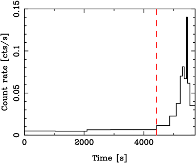
Figure 1: X-ray light curve for source LSPM J0501+2237 showing a strong X-ray flare towards the end of the observation. The red dashed line shows the time after which the data was excluded from analysis.

2.4 Spectral fitting and X-ray fluxes

The extracted source spectra were fitted with thermal plasma X-ray spectral models using xspec version 12.6.0 (Arnaud, 1996). The spectra were compared to apec (Smith et al., 2001) single-temperature models (Raymond & Smith, 1977) in collisional ionization equilibrium and absorbed by a hydrogen column using the tbabs xspec model (Balucinska-Church & McCammon, 1992). Due to the proximity of these objects we set the maximum hydrogen column density to be $10^{21}$ cm^-2 ($A_{V}\sim 0.5$, though the fitted values were much lower than this). A grid of initial thermal plasma temperatures covering $kT=0.1-3.0$ keV was used to prevent fitting local minima, and then the model with the lowest C-statistic (Cash, 1979) was selected as the best fit for each source. Only single-temperature thermal plasma models were tried for these sources as the number of photon events extracted (3 – 130) was not high enough for more complex fits.

The results of the spectral fits, including thermal plasma temperatures and absorption-corrected broad band (0.5–8.0 keV) fluxes, are provided in Table 1. The uncertainties on the X-ray fluxes take into account the model fitting uncertainties as well as the uncertainties on the measured net counts. Fractional X-ray luminosities, $L_{X}/L_{bol}$, were calculated using the bolometric luminosities calculated earlier. The plasma temperatures are mostly in the range 0.3–0.9 keV, which are consistent with those found for other M-type dwarf stars and X-ray faint field stars (e.g., Micela et al., 1997; Wright et al., 2010), although one star, 2MASS J19310458-0306, has a surprisingly high (but poorly constrained) plasma temperature of 2.2${}^{+2.4}_{-0.8}$ keV.

2.5 ROSAT observations of additional sources

Two objects, GJ 699 and GJ 551, were observed by ROSAT, with X-ray fluxes presented by Schmitt & Liefke (2004). These have been included in our sample and their stellar and X-ray properties are presented in Table 1.

2.6 Homogenisation of existing data for fully convective stars

To facilitate reliable comparisons between the sources observed for this study and the fully convective (but rapidly-rotating) stars include in the catalogue of Wright et al. (2011) we have reprocessed those sources in the same manner as our new targets. This comprised calculating $J$-band bolometric corrections from the $V-J$ colour and the equations of Mann et al. (2015) for calculating bolometric luminosities and calculating stellar masses from $M_{K}$ and the equations of Benedict et al. (2016). The X-ray luminosities and rotation periods presented by Wright et al. (2011) remain unchanged.

Since the Wright et al. (2011) catalogue (and the majority of the original X-ray papers used in that work) do not provide individual X-ray flux uncertainties we adopt a standard 20% uncertainty on X-ray flux (see discussion of typical sources of uncertainty in calculating X-ray fluxes in Jeffries et al., 2011), in addition to photometric uncertainties of 0.2 mag in $V$ (Hartman et al., 2011) and 0.1 mag for the near-IR photometry (Skrutskie et al., 2006). Given that all the fully convective sources from Wright et al. (2011) have saturated X-ray emission, their uncertainties on $L_{X}/L_{bol}$ and Rossby number will not significantly affect our results.

3 Rotation – activity relationship

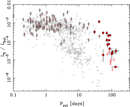
Figure 2: X-ray to bolometric luminosity ratio, $L_{X}/L_{bol}$, plotted against the rotation period, $P_{rot}$, for the fully convective stars observed as part of this work (large red points), the fully convective stars included in the sample of Wright et al. (2011, medium, light red points), and the remaining partly convective stars from that sample (grey empty circles). Error bars are shown for all fully convective stars. Upper (3$\sigma$) limits are shown for the undetected fully convective stars observed as part of this work as red arrows.

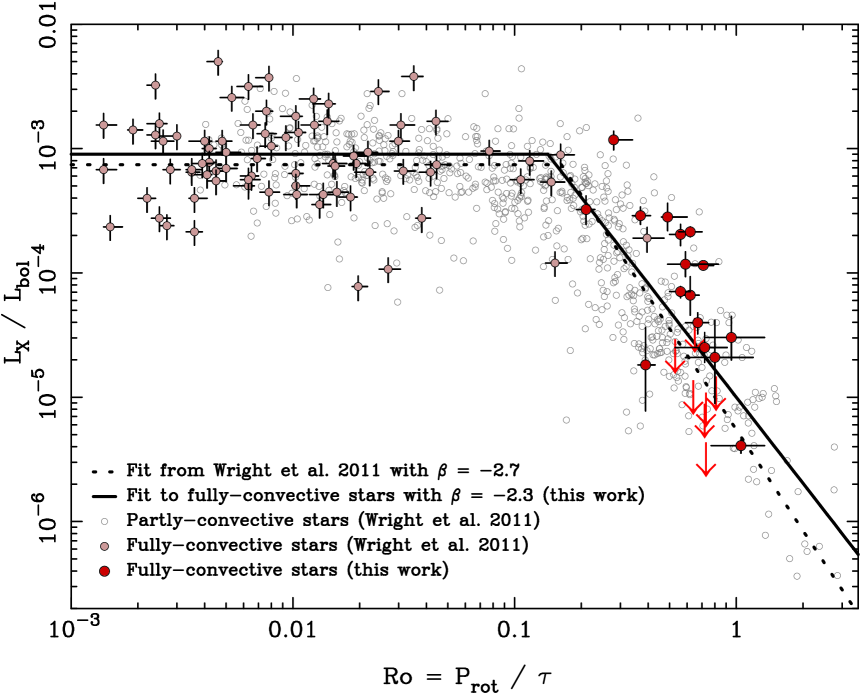
Figure 3: X-ray to bolometric luminosity ratio, $L_{X}/L_{bol}$, plotted against the Rossby number, $\mathrm{Ro}=P_{rot}/\tau$, for the fully convective stars observed as part of this work (large red points), the fully convective stars included in the sample of Wright et al. (2011, medium, light red points), and the remaining partly convective stars from that sample (grey empty circles). Error bars are shown for all fully convective stars. Upper (3$\sigma$) limits are shown for the undetected fully convective stars observed as part of this work as red arrows. The best-fitting activity - rotation relations found for fully convective stars in this work ($\beta=-2.3$ and $\mathrm{Ro}_{sat}=0.14$, solid line) and from Wright et al. (2011, $\beta=-2.7$ and $\mathrm{Ro}_{sat}=0.16$, dotted line) are shown.

In this Section we study the relationship between rotation and X-ray activity in our sample of fully-convective stars. The relationship between fractional X-ray luminosity and rotation period is shown in Figure 2 and with Rossby number (the ratio of the rotation period to the convective turnover time, $\tau$) is shown in Figure 3. For the latter we have initially adopted the empirically-calibrated convective turnover times from Wright et al. (2011), allowing us to place both partly- and fully-convective stars on the same rotation-activity diagram, and then use the apparent universality of the relationship to refine this empirical calibration. The use of empirically-determined convective turnover times does introduce a risk that they will hide interesting features in the original data (shown in Figure 2) though we note that this will not influence the fitted slope in the unsaturated regime. This is because any change to $\tau$ will cause stars of a similar colour or spectral type to shift to lower or higher Rossby numbers by a fixed amount in log space. Since our sample of fully-convective stars does not show a correlation between colour and rotation period this shift should not affect the fitted slope, and vice versa.

3.1 Fitting a rotation – activity relationship for fully convective stars

Figure 3 shows the standard rotation – activity diagram with the fractional X-ray luminosity, $L_{X}/L_{bol}$, plotted against the Rossby number, $\mathrm{Ro}=P_{rot}/\tau$ for all the fully-convective stars in our sample, both new targets and those presented by Wright et al. (2011). The figure also shows the positions of partly-convective stars from Wright et al. (2011) that define the well-known rotation – activity relationship: rapid rotators (those with Rossby numbers less than $\sim$0.1) show saturated activity at a level of $L_{X}/L_{bol}\sim 10^{-3}$, while slower rotators exhibit a power-law dependence between the fractional X-ray luminosity and the Rossby number. The new fully convective stars observed as part of this work appear to follow the same rotation-activity relationship known for partly convective stars (Wright & Drake, 2016).

To determine whether the slope of the rotation-activity relationship for fully-convective stars is different to that for partly-convective stars, we fit the distribution of fully-convective stars in the rotation-activity diagram with the traditional two-part power-law function commonly used for this purpose (e.g., Pizzolato et al., 2003; Wright et al., 2011). This has the form

$$\frac{L_{X}}{L_{bol}}=\left\{\begin{array}[]{ll}C\,Ro^{\beta}&\textrm{if $\mathrm{Ro}>\mathrm{Ro}_{sat}$}\\ \left(\frac{L_{X}}{L_{bol}}\right)_{sat}&\textrm{if $\mathrm{Ro}\leq\mathrm{Ro}_{sat}$}\end{array}\right.$$ (1)

where $(L_{X}/L_{bol})_{sat}$ is the fractional X-ray luminosity for saturated stars, $\beta$ is the power-law slope for the unsaturated part of the rotation-activity relationship, $\mathrm{Ro}_{sat}$ is the Rossby number at which X-ray saturation occurs, and $C$ is a constant.

We fit this relationship using Bayesian inference and forward modelling, allowing us to model the X-ray activity levels of all the observed stars according to their rotation periods, convective turnover times, and the rotation-activity relationship in equation 1. By forward modelling our observations and fitting their measured X-ray count rates to those predicted by our model we can also include and fit the 7 undetected sources (shown in Figure 3 as upper limits) based on the number of net X-ray counts calculated from source extraction performed at their expected source positions.

Our likelihood model starts by calculating Rossby numbers for our targets from their measured rotation periods and convective turnover times calculated from their $V-K_{s}$ colour and the relationship in Wright et al. (2011). From this and the rotation-activity relationship in equation 1 we predict a fractional X-ray luminosity for each source. X-ray fluxes were then predicted using the bolometric luminosities as described in Section 2.1. For the sources observed in this study the X-ray fluxes were then converted to X-ray count rates using the xspec model fits performed in Section 2.4 appropriate for each observation. For the fully convective stars included in the Wright et al. (2011) catalogue, for which X-ray count rates are unavailable for most sources, we performed the comparison with their X-ray fluxes.

To introduce both measurement uncertainties for measured quantities (photometry, rotation periods, and coronal plasma temperatures) as well as calibration uncertainties for inferred quantities (convective turnover times and bolometric corrections) we treat the true values of these quantities as nuisance parameters. We are effectively sampling a function, $P(\theta,\phi|x)$, that can be expanded as

$$P(\theta,\phi\,|\,x)=P(\theta\,|\,\phi,x)\,\,P(\phi\,|\,x)$$ (2)

where $\theta$ are the parameters of interest, $\phi$ are the nuisance parameters (the uncertain measurements and inferred quantities), and $x$ are the observations. We then decouple $\phi$ from its dependence on the data, assuming that $P(\phi)=P(\phi|x)$, i.e., the full observations are not informative on these nuisance parameters compared to our prior knowledge. This then reduces our function to

$$P(\theta,\phi\,|\,x)=P(\theta\,|\,\phi,x)\,\,P(\phi)$$ (3)

allowing us to marginalise out the nuisance parameters. We implement this using a two-step process following the method of Lee et al. (2011), first sampling from $P(\phi)$ and then iterating several times, each time sampling from $P(\theta|\phi,x)$, before resampling from $P(\phi)$. The number of sub-iterations required to generate independent draws is typically $n=10$ (Lee et al., 2011), but can be verified by inspecting the time series plots for different parameters ($\theta)$ to check there is no strong dependency on $\phi$ by the $n^{th}$ iteration.

The model has three free parameters; the logarithm of the saturation values of the fractional X-ray luminosity, log $(L_{X}/L_{bol})_{sat}$, the power-law slope in the saturated regime, $\beta$, and the constant log $C$ (that effectively sets the saturation threshold, $\mathrm{Ro}_{sat}$). A fourth parameter ($f$) was introduced to represent the scatter in the rotation-activity diagram, which may be due to a combination of inherent X-ray variability and underestimated uncertainties on various parameters (see Hogg et al., 2010). We marginalised over $f$ to calculate uncertainties on the other fit parameters. Wide and uniform priors of $-5<\mathrm{log}(L_{X}/L_{bol})_{sat}<-1$, $-10<\beta<0$, and $-8<\mathrm{log}C<-1$ were used.

To sample the posterior distribution function we use the affine-invariant MCMC ensemble sampler (Goodman & Weare, 2010) emcee (Foreman-Mackey et al., 2013), using 10,000 walkers, a total of 2000 iterations, discarding the first half as a burn-in, and a sub-iteration cadence of 10 iterations, with no evidence for a dependence between $\phi$ and $\theta$. The three parameters have very similar autocorrelation lengths with the longest being the constant $C$ of 13.9 iterations, resulting in $\sim$72 independent samples per walker. The posterior distribution functions were found to follow a normal distribution, and thus the median value was used as the best fit, with the 16^th and 84^th percentiles used for the 1$\sigma$ uncertainties.

The best fit slope to the unsaturated regime was found to be $\beta=-2.3^{+0.4}_{-0.6}$, which is between the canonical $\beta=-2$ value and the value of $\beta=-2.7$ found by Wright et al. (2011) from their X-ray unbiased subsample (since we have been able to include upper limits for all our undetected sources, we have no reason to think that non-detections will bias our results), though the uncertainties are sufficiently large as to be consistent with both values. This result rules out there being no dependency between Rossby number and $L_{X}/L_{bol}$ for fully convective stars to a confidence of $\sim$6$\sigma$. The saturation threshold for fully convective stars is estimated to be $\mathrm{Ro}_{sat}=0.14^{+0.08}_{-0.04}$ and the saturation value is log $(L_{X}/L_{bol})_{sat}=-3.05^{+0.05}_{-0.06}$, both of which are fully consistent with the values of $\mathrm{Ro}_{sat}=0.13\pm 0.02$ (for $\beta=-2$) or $\mathrm{Ro}_{sat}=0.16\pm 0.03$ (for $\beta=-2.7$), and log $(L_{X}/L_{bol})_{sat}=-3.13$ found by Wright et al. (2011) for a sample predominantly composed of partly-convective stars. Figure 3 shows the best fit activity-rotation relationship compared to that of Wright et al. (2011).

3.2 Dependence of the rotation – activity relationship on $V-K_{s}$ colour

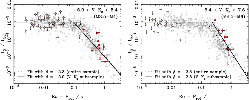
Figure 4: X-ray to bolometric luminosity ratio, $L_{X}/L_{bol}$, plotted against the Rossby number, $\mathrm{Ro}=P_{rot}/\tau$, for two subsamples of our fully convective star sample, divided based on the $V-K_{s}$ colour. Symbol colour is the same as in Figure 3: fully convective stars from this work are shown as large red circles, from Wright et al. (2011) shown as medium, light red circles, and partly convective stars are shown as empty grey circles. Error bars and 3$\sigma$ upper limits are also shown. The best-fitting activity - rotation relations found for the entire sample of fully convective stars ($\beta=-2.3$, dotted line) is shown compared to the fits for each subsample, $\beta=-2.0$ (for $V-K_{s}<5.4$) and $\beta=-2.8$ (for $V-K_{s}>5.4$).

Previous studies of the rotation-activity relationship have not found any significant variation in the slope of the unsaturated regime as a function of stellar, mass, or colour (e.g., Pizzolato et al., 2003; Wright et al., 2011; Newton et al., 2017). However, this is the first time that the unsaturated regime of the rotation - coronal activity relationship has been explored for fully-convective stars, and as such any variation in the slope of the unsaturated regime could provide important clues to the dynamo mechanism at work in such stars.

We divide our sample into two approximately-equal halves based on $V-K_{s}$ colour. These two samples, the ‘blue’ (12 stars from our new sample with $V-K_{s}<5.4$) and ‘red’ (11 stars from our new sample with $V-K_{s}>5.4$) fully-convective stars, are shown in Figure 4 alongside the other stars that meet these criteria from Wright et al. (2011, all in the saturated regime). We then fit two-part activity-rotation relationships exactly as in Section 3.1, as shown in Figure 4.

We find that the two samples exhibit slopes in the unsaturated regime with power-law indexes of $\beta=-2.0^{+0.7}_{-0.4}$ (blue sample) and $\beta=-2.8^{+0.6}_{-0.8}$ (red sample), that are consistent with each other within the uncertainties (the other fit parameters are also all consistent between the fits). We thus find no significant evidence for a variation in the rotation-activity relationship for fully-convective stars of different mass or radius, although actual differences might be masked by incorrectly-calibrated convective turnover times (the values we have used from Wright et al., 2011, are poorly constrained for fully convective stars due to the lack of such stars in the unsaturated regime of their sample).

3.3 Empirical determination of the convective turnover time for fully convective stars

While stellar convective turnover times can be calculated theoretically (e.g., Kim & Demarque, 1996; Ventura et al., 1998), it is also possible to estimate them empirically (e.g., Noyes et al., 1984; Stepien, 1994; Pizzolato et al., 2003; Wright et al., 2011), based on the assumption of a universal rotation-activity relationship for active stars. However, due to the lack of previously known X-ray unsaturated fully convective stars it has been impossible to do this for fully convective stars, with earlier estimates based only on stars in the saturated regime (Wright et al., 2011). Using our data for X-ray unsaturated fully convective stars we revisit the empirical convective turnover times presented by Wright et al. (2011) and improve their estimates for fully convective stars.

To do this we follow the method of Stepien (1994) and Wright et al. (2011) by fitting two-part rotation-activity relationships in the $L_{X}/L_{bol}$–$P_{rot}$ diagram for subsamples of stars based on their colour. The fitted relationship is of the form

$$\frac{L_{X}}{L_{bol}}=\left\{\begin{array}[]{ll}C_{P}\,P_{rot}^{\beta}&\textrm{if $P_{rot}>P_{sat}$}\\ \left(\frac{L_{X}}{L_{bol}}\right)_{sat}&\textrm{if $P_{rot}\leq P_{sat}$}\end{array}\right.$$ (4)

which is exactly the same as that in equation 1, but with $P_{rot}$ instead of Rossby number as the main dependent. On the assumption of a universal activity-rotation relationship we fix the parameters $\beta=-2.7$ and log $(L_{X}/L_{bol})_{sat}=-3.13$ according to the best-fitting relationship found by Wright et al. (2011) and with which our new fully convective stars are consistent. This leaves only one free parameter, the rotation period saturation threshold, $P_{sat}$ (since the constant is given by $C_{P}=(L_{X}/L_{bol})_{sat}\,P_{sat}^{-\beta}$). As in Section 3.1 we fit this relationship using Bayesian inference, use the MCMC ensemble sampler emcee to sample the posterior distribution, and add an extra parameter ($f$) to represent the scatter in the relationship.

We perform these fits for colour bins of approximately the same width as those used by Wright et al. (2011) using the same sample as those authors, but complemented with the additional stars included in this study. The reddest bin was replaced with two bins to better explore how the convective turnover time varies for fully-convective stars of different colour. These bins were chosen, as in Section 3.2, to divide the sample of unsaturated fully convective stars in two. The bins in $V-K_{s}$ colour, the number of stars in each bin, and the convective turnover times determined from our fitting process are listed in Table 2.

$V-K_{s}$		Mass / $M_{\odot}$		$N_{\star}$	log $\tau$
range	med.	range	med.		(days)
1.00 – 1.46	1.42	1.15 – 1.36	1.17	89	$0.93^{+0.04}_{-0.05}$
1.46 – 1.85	1.64	1.00 – 1.14	1.09	80	$1.12^{+0.05}_{-0.04}$
1.85 – 2.17	2.00	0.90 – 0.99	0.95	80	$1.17^{+0.04}_{-0.04}$
2.17 – 2.84	2.54	0.77 – 0.89	0.83	82	$1.36^{+0.04}_{-0.04}$
2.84 – 3.37	3.14	0.65 – 0.76	0.70	80	$1.42^{+0.05}_{-0.04}$
3.37 – 3.69	3.53	0.57 – 0.64	0.61	84	$1.52^{+0.04}_{-0.05}$
3.69 – 4.15	3.88	0.37 – 0.56	0.50	83	$1.72^{+0.06}_{-0.05}$
4.15 – 4.59	4.37	0.25 – 0.36	0.30	80	$1.82^{+0.08}_{-0.06}$
4.59 – 4.91	4.74	0.21 – 0.24	0.22	80	$1.96^{+0.07}_{-0.08}$
4.91 – 5.44	5.14	0.16 – 0.20	0.18	73	$2.07^{+0.05}_{-0.05}$
5.44 – 7.00	5.63	0.08 – 0.15	0.14	35	$2.19^{+0.05}_{-0.05}$

Table 2: Empirical convective turnover times fitted from the combination of the data presented here and those from Wright et al. (2011). Fits were performed under the assumption of a universal activity-rotation relationship with $\beta=-2.70$, as determined by Wright et al. (2011). The median value of the posterior distribution was used as the best fit and the 16^th and 84^th percentiles used to determine the 1$\sigma$ uncertainties. Stellar masses were estimated using the empirical data in Pecaut & Mamajek (2013) to convert $V-K_{s}$ to $T_{eff}$ and a 1 Gyr isochrone from Siess et al. (2000) to convert to stellar mass, as per Wright et al. (2011).

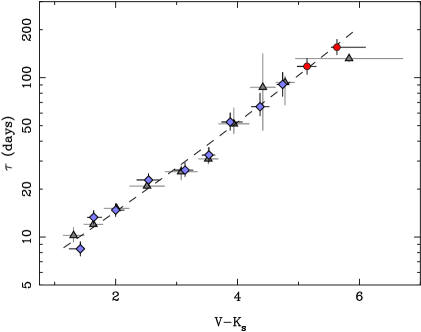
Figure 5: Empirical convective turnover time as a function of $V-K_{s}$ colour using the best-fitting activity-rotation model parameters determined by Wright et al. (2011) with $\beta=-2.70$ and log $(L_{X}/L_{bol})_{sat}=-3.13$. Error bars (1$\sigma$) are shown for all points, which for $V-K_{s}$ colour are the 16^th-84^th percentiles of the colour distribution within each bin. Grey triangles show the convective turnover times determined by Wright et al. (2011), while blue diamonds and red circles show the values determined in this work for partly-convective stars (data entirely from Wright et al., 2011) and for fully-convective stars (data from that paper and this work), respectively. The slight differences between the results of this work and Wright et al. (2011) for partly-convective stars can be attributed to the different fitting techniques employed. The dashed line shows the best-fitting polynomial relationship between the two quantities.

Figure 5 shows the best-fitting convective turnover times determined as a function of $V-K_{s}$ colour and compared to those determined previously by Wright et al. (2011). Our estimates of the convective turnover times for partly-convective stars differ slightly from those determined by Wright et al. (2011), which can be attributed to slight differences in the fitting technique (we fixed the $L_{X}/L_{bol}$ saturation level and introduced a free parameter to account for the large scatter in the rotation-activity relationship, which those authors did not). For fully convective stars we see that the convective turnover time continues to rise, with no evidence for the flattening-off hinted at in the results of Wright et al. (2011). Note that the slightly lower convective turnover time we find at the blue end may not be real as it may be caused by the onset of super-saturation for rapidly-rotating F-type stars (see Figure 6 of Wright et al., 2011).

We parameterise these results by fitting various polynomial functions to log $\tau$ as a function of $V-K_{s}$. We fit these functions using MCMC, varying $V-K_{s}$ for each fit in accordance with the distribution of values within each bin. We find a good fit with a simple straight line, with no evidence that either higher-order polynomials or multi-part functions are necessary for a better fit. The best fit is

$$\mathrm{log}\tau=0.64^{+0.10}_{-0.12}+0.25^{+0.08}_{-0.07}(V-K_{s})$$ (5)

which is valid over the range $1.1<V-K_{s}<7.0$ and has an rms dispersion in log $\tau$ of 0.045 dex. This parameterisation of $\tau$ should replace the equivalent fit in Wright et al. (2011), which was highly uncertain for $V-K_{s}>5$ due to their lack of unsaturated fully-convective stars. Converting the $V-K_{s}$ colours to $T_{eff}$ using the data from Pecaut & Mamajek (2013) and converting these to stellar mass using a 1 Gyr iscohrone from Siess et al. (2000) we can also parameterise $\tau$ in terms of stellar mass (see Table 2) and fit a polynomial relationship of the form

$$\mathrm{log}\tau=2.33^{+0.06}_{-0.05}-1.50^{+0.21}_{-0.20}(M/M_{\odot})+0.31^{+0.16}_{-0.17}(M/M_{\odot})^{2}$$ (6)

which is valid over the range $0.08<M/M_{\odot}<1.36$ and has an rms dispersion in log $\tau$ of 0.055 dex. More complex functions were explored but did not provide a better fit.

4 Discussion

We have measured X-ray luminosities for an expanded sample of slowly-rotating, fully-convective stars so that they can be plotted in an X-ray activity - rotation diagram to study correlations between the two quantities. We find that the sources follow the classical rotation – activity relationship known for partly-convective stars and hinted at in the study of Wright & Drake (2016), with a power-law relationship between Rossby number and fractional X-ray luminosity for slow rotators and a saturated fractional X-ray luminosity for fast rotators. With our expanded sample we are able to quantify the power-law slope in the unsaturated regime for the first time and fit a value of $\beta=-2.3^{+0.4}_{-0.6}$, consistent with that found for partly convective stars of $\beta=-2.70\pm 0.13$ by Wright et al. (2011). There is a hint that the slope may vary as a function of $V-K_{s}$ colour for the fully-convective stars, but this is equally-well explained by (and probably more likely due to) variations in the convective turnover time.

Since the rotation - activity relationship is believed to be a proxy for the underlying magnetic dynamo, this similarity between the form of the relationships for partly- and fully-convective stars is surprising because the two types of star have long been thought to operate very different magnetic dynamos (e.g., Durney et al., 1993). As discussed by Wright & Drake (2016) the most likely explanations for this are either that fully convective stars operate the same dynamo to that found in partly-convective stars like the Sun (which would therefore require that the tachocline is not a vital ingredient for such a dynamo) or that fully convective stars generate a purely turbulent dynamo (one that does not rely on a shear layer) that exhibits a rotation-activity relationship very similar to that in partly-convective stars.

Turbulent dynamos are those that do not rely on a shear layer and are sometimes referred to as $\alpha^{2}$ dynamos. Durney et al. (1993) were among the first to explore their potential, finding that they would produce a small-scale magnetic field in fully-convective stars, but that a large-scale field could not be generated without a shear layer. Such models were only weakly dependent on rotation and could not provide the rotation-activity relationship we see in Figure 3. Later 3D dynamo simulations by Dobler et al. (2006) and Browning (2008) were able to generate larger-scale magnetic fields with some evidence that rotation may influence the resulting magnetic field strength. More recent 3D dynamo simulations of M-type stars without a tachocline have been able to reproduce both cyclic behaviour on 5–15 year timescales (Fan & Fang, 2014), the detailed small-scale and large-scale features of magnetic fields in fully convective stars (Yadav et al., 2015), and decreases in field strength and emergence of magnetic cycles at slow rotation periods (Yadav et al., 2016). The latter feature is in line with recent reporting of activity cycles in late-type stars without a tachocline (Route, 2016; Wargelin et al., 2017). While such a dynamo could produce the observed trend between rotation and X-ray activity that we have observed, it is perhaps surprising that two very different dynamo mechanisms would have the same relationship between these two quantities.

An alternative hypothesis is that fully-convective stars actually operate a dynamo very similar to that found in our Sun. Spruit (2011) has argued that both observations and simple theoretical considerations point to the solar convection zone as the only necessary ingredient for dynamo action. The Solar dynamo requires a layer of strong shear to induce the $\Omega$ effect that converts the poloidal field to a toroidal field. Regions of strong shear do exist within stellar convection zones, but since magnetic flux tubes are highly buoyant it has been suggested that this would not provide sufficient time for the magnetic field to be amplified to sufficient strength before it rises to the surface (Parker, 1975). At the bottom of the convection zone the tachocline provides a layer of strong shear where magnetic buoyancy is weak and as such the field can be sufficiently amplified before it reaches the stellar surface. However, current 3D dynamo simulations have found that differential rotation within the convection zone of stars can generate large-scale toroidal magnetic fields through the $\Omega$ effect without the need for a tachocline (e.g., Muñoz-Jaramillo et al., 2009; Brown et al., 2010; Nelson et al., 2013; Yadav et al., 2015, 2016). These distributed dynamo models may suggest that previous interface dynamo models, where the toroidal field is generated just at the tachocline, are not necessary.

Most dynamo models are not at the stage where they can predict correlations between rotation and either magnetic field strength or magnetic activity indicators such as X-ray activity. As theory progresses observational constraints such as the form of the rotation-activity relationship for fully-convective stars are vital for identifying the key features such dynamos should exhibit and how they differ (or not) to those in solar-like stars.

5 Conclusions

We have combined new X-ray observations of 19 slowly-rotating fully-convective stars with existing X-ray data and rotation periods from various sources. From the resulting X-ray luminosities and upper limits we have produced the first X-ray activity-rotation diagram for fully convective stars that is well populated in both the saturated and unsaturated regimes. We confirm the results of Wright & Drake (2016) that fully-convective stars exhibit a rotation-activity relationship that is indistinguishable from that of partly-convective stars. We measure the power-law slope of the relationship between Rossby number and fractional X-ray luminosity for X-ray unsaturated fully-convective stars for the first time, and find it to be consistent with that measured for partly-convective stars. We then use this data to improve the empirical estimation of the convective turnover time for fully-convective stars, which was previously poorly constrained.

Our results suggest that either fully-convective stars operate a turbulent dynamo that leads to a rotation-activity relationship with the same dependence on Rossby number as that for partly-convective stars, or that both types of star operate very similar dynamos that rely on the interaction of rotation and turbulent convection. We suggest that the latter explanation is more likely, especially in the light of recent models that have shown that $\alpha\Omega$ dynamos can operate without the aid of a tachocline, with the shearing action distributed throughout the convective envelope instead of being concentrated in the interface between the radiative core and the convective envelope.

6 Acknowledgments

We thank the anonymous referee for a careful and helpful reading of the paper as well as comments and suggestions that have improved the quality of this paper. NJW acknowledges an STFC Ernest Rutherford Fellowship (grant number ST/M005569/1). ERN is supported by an NSF Astronomy and Astrophysics Postdoctoral Fellowship under award AST-1602597. JJD was supported by NASA contract NAS8-03060 to the Chandra X-ray Center and thanks the director, H. Tananbaum, and the science team for continuing support and advice. This research has made use of data from the Chandra X-ray Observatory and software provided by the Chandra X-ray Center in the application packages CIAO and Sherpa, and from Penn State for the ACIS Extract software package. This research has also made use of NASA’s Astrophysics Data System and the Simbad and VizieR databases, operated at CDS, Strasbourg.

References

- Arnaud (1996) Arnaud K. A., 1996, in ASP Conference Series, Jacoby G. H., Barnes J., eds., Vol. 101, p. 17
- Astudillo-Defru et al. (2017) Astudillo-Defru N., Delfosse X., Bonfils X., Forveille T., Lovis C., Rameau J., 2017, A&A, 600, A13
- Balucinska-Church & McCammon (1992) Balucinska-Church M., McCammon D., 1992, ApJ, 400, 699
- Benedict et al. (2016) Benedict G. F. et al., 2016, AJ, 152, 141
- Benedict et al. (1999) Benedict G. F. et al., 1999, AJ, 118, 1086
- Benedict et al. (1998) Benedict G. F. et al., 1998, AJ, 116, 429
- Broos et al. (2010) Broos P. S., Townsley L. K., Feigelson E. D., Getman K. V., Bauer F. E., Garmire G. P., 2010, ApJ, 714, 1582
- Brown et al. (2010) Brown B. P., Browning M. K., Brun A. S., Miesch M. S., Toomre J., 2010, ApJ, 711, 424
- Browning (2008) Browning M. K., 2008, ApJ, 676, 1262
- Caramazza et al. (2007) Caramazza M., Flaccomio E., Micela G., Reale F., Wolk S. J., Feigelson E. D., 2007, A&A, 471, 645
- Cash (1979) Cash W., 1979, ApJ, 228, 939
- Chabrier & Baraffe (1997) Chabrier G., Baraffe I., 1997, A&A, 327, 1039
- Charbonneau (2010) Charbonneau P., 2010, Living Reviews in Solar Physics, 7, 3
- Cutri et al. (2003) Cutri R. M. et al., 2003, 2MASS All Sky Catalog of point sources. The IRSA 2MASS All-Sky Point Source Catalog
- David & Hillenbrand (2015) David T. J., Hillenbrand L. A., 2015, ApJ, 804, 146
- Delfosse et al. (1998) Delfosse X., Forveille T., Perrier C., Mayor M., 1998, A&A, 331, 581
- Dikpati & Charbonneau (1999) Dikpati M., Charbonneau P., 1999, ApJ, 518, 508
- Dittmann et al. (2014) Dittmann J. A., Irwin J. M., Charbonneau D., Berta-Thompson Z. K., 2014, ApJ, 784, 156
- Dobler et al. (2006) Dobler W., Stix M., Brandenburg A., 2006, ApJ, 638, 336
- Durney et al. (1993) Durney B. R., De Young D. S., Roxburgh I. W., 1993, Solar Physics, 145, 207
- Fan & Fang (2014) Fan Y., Fang F., 2014, ApJ, 789, 35
- Feigelson et al. (2004) Feigelson E. D. et al., 2004, ApJ, 611, 1107
- Finch & Zacharias (2016) Finch C. T., Zacharias N., 2016, AJ, 151, 160
- Flaccomio et al. (2005) Flaccomio E., Micela G., Sciortino S., Feigelson E. D., Herbst W., Favata F., Harnden, Jr. F. R., Vrtilek S. D., 2005, ApJS, 160, 450
- Foreman-Mackey et al. (2013) Foreman-Mackey D., Hogg D. W., Lang D., Goodman J., 2013, PASP, 125, 306
- Fruscione et al. (2006) Fruscione A. et al., 2006, in Proceedings of SPIE, Volume 6270, pp. 62701V, Vol. 6270
- Garmire et al. (2003) Garmire G. P., Bautz M. W., Ford P. G., Nousek J. A., Ricker, Jr. G. R., 2003, in Proceedings of SPIE, J. E. Truemper & H. D. Tananbaum, ed., Vol. 4851, pp. 28–44
- Giclas et al. (1971) Giclas H. L., Burnham R., Thomas N. G., 1971, Lowell proper motion survey Northern Hemisphere. Lowell Observatory
- Gliese & Jahreiß (1979) Gliese W., Jahreiß H., 1979, A&AS, 38
- Goodman & Weare (2010) Goodman J., Weare J., 2010, Comm. App. Math. Comp. Sci., 5, 65
- Hartman et al. (2011) Hartman J. D., Bakos G. Á., Noyes R. W., Sipőcz B., Kovács G., Mazeh T., Shporer A., Pál A., 2011, AJ, 141, 166
- Hawley (1993) Hawley S. L., 1993, PASP, 105, 955
- Hawley et al. (1996) Hawley S. L., Gizis J. E., Reid I. N., 1996, AJ, 112, 2799
- Henry et al. (2006) Henry T. J., Jao W.-C., Subasavage J. P., Beaulieu T. D., Ianna P. A., Costa E., Méndez R. A., 2006, AJ, 132, 2360
- Hogg et al. (2010) Hogg D. W., Bovy J., Lang D., 2010, ArXiv e-prints
- Irwin et al. (2011) Irwin J., Berta Z. K., Burke C. J., Charbonneau D., Nutzman P., West A. A., Falco E. E., 2011, ApJ, 727, 56
- Jeffries et al. (2011) Jeffries R. D., Jackson R. J., Briggs K. R., Evans P. A., Pye J. P., 2011, MNRAS, 411, 2099
- Jenkins et al. (2009) Jenkins J. S., Ramsey L. W., Jones H. R. A., Pavlenko Y., Gallardo J., Barnes J. R., Pinfield D. J., 2009, ApJ, 704, 975
- Johns-Krull & Valenti (1996) Johns-Krull C. M., Valenti J. A., 1996, ApJL, 459, L95
- Jouve et al. (2010) Jouve L., Brown B. P., Brun A. S., 2010, A&A, 509, A32
- Kim & Demarque (1996) Kim Y.-C., Demarque P., 1996, ApJ, 457, 340
- Kiraga (2012) Kiraga M., 2012, Acta Astronomica, 62, 67
- Lee et al. (2011) Lee H. et al., 2011, ApJ, 731, 126
- Lépine & Gaidos (2011) Lépine S., Gaidos E., 2011, AJ, 142, 138
- Lépine & Shara (2005) Lépine S., Shara M. M., 2005, AJ, 129, 1483
- Luyten (1942) Luyten W. J., 1942, Publications of the Astronomical Observatory University of Minnesota, 2, 242
- Mann et al. (2015) Mann A. W., Feiden G. A., Gaidos E., Boyajian T., von Braun K., 2015, ApJ, 804, 64
- Mann et al. (2016) Mann A. W., Feiden G. A., Gaidos E., Boyajian T., von Braun K., 2016, ApJ, 819, 87
- Mermilliod (1986) Mermilliod J.-C., 1986, Catalogue of Eggen’s UBV data., 0 (1986)
- Micela et al. (1997) Micela G., Pye J., Sciortino S., 1997, A&A, 320, 865
- Micela et al. (1985) Micela G., Sciortino S., Serio S., Vaiana G. S., Bookbinder J., Golub L., Harnden, Jr. F. R., Rosner R., 1985, ApJ, 292, 172
- Mohanty & Basri (2003) Mohanty S., Basri G., 2003, ApJ, 583, 451
- Monet et al. (2003) Monet D. G. et al., 2003, AJ, 125, 984
- Morin et al. (2010) Morin J., Donati J.-F., Petit P., Delfosse X., Forveille T., Jardine M. M., 2010, MNRAS, 407, 2269
- Muñoz-Jaramillo et al. (2009) Muñoz-Jaramillo A., Nandy D., Martens P. C. H., 2009, ApJ, 698, 461
- Nelson et al. (2013) Nelson N. J., Brown B. P., Brun A. S., Miesch M. S., Toomre J., 2013, ApJ, 762, 73
- Newton et al. (2017) Newton E. R., Irwin J., Charbonneau D., Berlind P., Calkins M. L., Mink J., 2017, ApJ, 834, 85
- Newton et al. (2018) Newton E. R., Irwin J., Charbonneau D., Berta-Thompson Z. K., 2018, Apj, in preparation
- Newton et al. (2016) Newton E. R., Irwin J., Charbonneau D., Berta-Thompson Z. K., Dittmann J. A., West A. A., 2016, ApJ, 821, 93
- Noyes et al. (1984) Noyes R. W., Hartmann L. W., Baliunas S. L., Duncan D. K., Vaughan A. H., 1984, ApJ, 279, 763
- Nutzman & Charbonneau (2008) Nutzman P., Charbonneau D., 2008, PASP, 120, 317
- Pallavicini et al. (1981) Pallavicini R., Golub L., Rosner R., Vaiana G. S., Ayres T., Linsky J. L., 1981, ApJ, 248, 279
- Parker (1955) Parker E. N., 1955, ApJ, 122, 293
- Parker (1975) Parker E. N., 1975, ApJ, 198, 205
- Pecaut & Mamajek (2013) Pecaut M. J., Mamajek E. E., 2013, ApJS, 208, 9
- Pizzolato et al. (2003) Pizzolato N., Maggio A., Micela G., Sciortino S., Ventura P., 2003, A&A, 397, 147
- Raymond & Smith (1977) Raymond J. C., Smith B. W., 1977, ApJS, 35, 419
- Reiners et al. (2012) Reiners A., Joshi N., Goldman B., 2012, AJ, 143, 93
- Reiners et al. (2014) Reiners A., Schüssler M., Passegger V. M., 2014, ApJ, 794, 144
- Riedel et al. (2010) Riedel A. R. et al., 2010, AJ, 140, 897
- Route (2016) Route M., 2016, ApJL, 830, L27
- Schmitt & Liefke (2004) Schmitt J. H. M. M., Liefke C., 2004, A&A, 417, 651
- See et al. (2015) See V. et al., 2015, MNRAS, 453, 4301
- Siess et al. (2000) Siess L., Dufour E., Forestini M., 2000, A&A, 358, 593
- Skrutskie et al. (2006) Skrutskie M. F., Cutri R. M., Stiening R., Weinberg M. D., Schneider S., Carpenter J. M., Beichman C., 2006, AJ, 131, 1163
- Skumanich (1972) Skumanich A., 1972, ApJ, 171, 565
- Smith et al. (2001) Smith R. K., Brickhouse N. S., Liedahl D. A., Raymond J. C., 2001, ApJL, 556, L91
- Spruit (2011) Spruit H. C., 2011, Theories of the Solar Cycle: A Critical View, Springer Netherlands, p. 39
- Stepien (1994) Stepien K., 1994, A&A, 292, 191
- Telleschi et al. (2007) Telleschi A., Güdel M., Briggs K. R., Audard M., Palla F., 2007, A&A, 468, 425
- Thompson et al. (1996) Thompson M. J. et al., 1996, Science, 272, 1300
- Vaiana et al. (1981) Vaiana G. S. et al., 1981, ApJ, 245, 163
- van Altena et al. (1995) van Altena W. F., Lee J. T., Hoffleit E. D., 1995, The general catalogue of trigonometric [stellar] parallaxes. Yale University Observatory
- Ventura et al. (1998) Ventura P., Zeppieri A., Mazzitelli I., D’Antona F., 1998, A&A, 334, 953
- Vilhu (1984) Vilhu O., 1984, A&A, 133, 117
- Wargelin et al. (2017) Wargelin B. J., Saar S. H., Pojmański G., Drake J. J., Kashyap V. L., 2017, MNRAS, 464, 3281
- Weber & Davis (1967) Weber E. J., Davis, Jr. L., 1967, ApJ, 148, 217
- Weinberger et al. (2016) Weinberger A. J., Boss A. P., Keiser S. A., Anglada-Escudé G., Thompson I. B., Burley G., 2016, AJ, 152, 24
- Weisskopf et al. (2002) Weisskopf M. C., Brinkman B., Canizares C., Garmire G., Murray S., Van Speybroeck L. P., 2002, PASP, 114, 1
- White et al. (1989) White S. M., Kundu M. R., Jackson P. D., 1989, A&A, 225, 112
- Winters et al. (2011) Winters J. G., Henry T. J., Jao W.-C., Subasavage J. P., Finch C. T., Hambly N. C., 2011, AJ, 141, 21
- Winters et al. (2015) Winters J. G. et al., 2015, AJ, 149, 5
- Winters et al. (2017) Winters J. G. et al., 2017, AJ, 153, 14
- Wright & Drake (2016) Wright N. J., Drake J. J., 2016, Nature, 535, 526
- Wright et al. (2010) Wright N. J., Drake J. J., Civano F., 2010, ApJ, 725, 480
- Wright et al. (2011) Wright N. J., Drake J. J., Mamajek E. E., Henry G. W., 2011, ApJ, 743, 48
- Yadav et al. (2015) Yadav R. K., Christensen U. R., Morin J., Gastine T., Reiners A., Poppenhaeger K., Wolk S. J., 2015, ApJL, 813, L31
- Yadav et al. (2016) Yadav R. K., Christensen U. R., Wolk S. J., Poppenhaeger K., 2016, ApJL, 833, L28
- Zacharias et al. (2013) Zacharias N., Finch C. T., Girard T. M., Henden A., Bartlett J. L., Monet D. G., Zacharias M. I., 2013, AJ, 145, 44