Coordinate-wise Powers of Algebraic Varieties

Abstract.

We introduce and study coordinate-wise powers of subvarieties of $\mathbb{P}^{n}$, i.e. varieties arising from raising all points in a given subvariety of $\mathbb{P}^{n}$ to the $r$-th power, coordinate by coordinate. This corresponds to studying the image of a subvariety of $\mathbb{P}^{n}$ under the quotient of $\mathbb{P}^{n}$ by the action of the finite group $\mathbb{Z}_{r}^{n+1}$. We determine the degree of coordinate-wise powers and study their defining equations, in particular for hypersurfaces and linear spaces. Applying these results, we compute the degree of the variety of orthostochastic matrices and determine iterated dual and reciprocal varieties of power sum hypersurfaces. We also establish a link between coordinate-wise squares of linear spaces and the study of real symmetric matrices with a degenerate eigenspectrum.

1. Introduction

Recently, Hadamard products of algebraic varieties have been attracting attention of geometers. These are subvarieties $X\star Y$ of projective space $\mathbb{P}^{n}$ that arise from multiplying coordinate-by-coordinate any two points $x\in X$, $y\in Y$ in given subvarieties $X,Y$ of $\mathbb{P}^{n}$. In applications, they first appeared in [CMS10], where the variety associated to the restricted Boltzmann machine was described as a repeated Hadamard product of the secant variety of $\mathbb{P}^{1}\times\ldots\times\mathbb{P}^{1}\subset\mathbb{P}^{2^{n}-1}$ with itself. Further study in [BCK16], [FOW17], [BCFL], [CCFL] made progress towards understanding Hadamard products.

Of particular interest are the $r$-th Hadamard powers $X^{\star r}:=X\star\ldots\star X$ of an algebraic variety $X\subset\mathbb{P}^{n}$. They are the multiplicative analogue of secant varieties that play a central role in classical projective geometry: The $r$-th secant variety $\sigma_{r}(X)$ is the closure of the set of coordinate-wise sums of $r$ points in $X$. Its subvariety corresponding to sums of $r$ equal points is the original variety $X$. In the multiplicative setting, the Hadamard power $X^{\star r}$ replaces $\sigma_{r}(X)$, but it does not typically contain $X$ if $[1:\ldots:1]\notin X$. As a multiplicative substitute for the inclusion $X\subset\sigma_{r}(X)$, it is natural to study the subvariety of $X^{\star r}$ given by coordinate-wise products of $r$ equal points in $X$.

Formally, for a projective variety $X\subset\mathbb{P}^{n}$ and an integer $r\in\mathbb{Z}$ (possibly negative), we are interested in studying its image under the rational map

$$\varphi_{r}\colon\mathbb{P}^{n}\dashrightarrow\mathbb{P}^{n},\qquad[x_{0}:\ldots:x_{n}]\mapsto[x_{0}^{r}:\ldots:x_{n}^{r}].$$

We call the image, $X^{\circ r}$, of $X$ under $\varphi_{r}$ the $r$-th coordinate-wise power of $X\subset\mathbb{P}^{n}$.

In this article, we investigate these coordinate-wise powers $X^{\circ r}$ with a main focus on the case $r>0$. These varieties show up naturally in many applications. For the Grassmannian variety $\operatorname{Gr}(k,\mathbb{P}^{n})$ in its Plücker embedding, the intersection with its $r$-th coordinate-wise power $\operatorname{Gr}(k,\mathbb{P}^{n})\cap\operatorname{Gr}(k,\mathbb{P}^{n})^{\circ r}$ was described combinatorially in terms of matroids in [Len17] for even $r$. In [Bon18], highly singular surfaces in $\mathbb{P}^{3}$ have been constructed as preimages of a specific singular surface under the morphism $\varphi_{r}$ for $r>0$. In the case $r=-1$, the map $\varphi_{r}$ is a classical Cremona transformation and images of varieties under this transformation are called reciprocal varieties whose study has received particular attention in the case of linear spaces, see [DSV12], [KV16] and [FSW18].

For $r>0$, the coordinate-wise powers $X^{\circ r}$ of a variety $X\subset\mathbb{P}^{n}$ have the following natural interpretation: The quotient of $\mathbb{P}^{n}$ by the finite subgroup $\mathbb{Z}_{r}^{n+1}$ of the torus $(\mathbb{C}^{*})^{n+1}$ is again a projective space. The image of a variety $X\subset\mathbb{P}^{n}$ in $\mathbb{P}^{n}/\mathbb{Z}_{r}^{n+1}\cong\mathbb{P}^{n}$ is the variety $X^{\circ r}$, since $\varphi_{r}\colon\mathbb{P}^{n}\to\mathbb{P}^{n}$ is the geometric quotient of $\mathbb{P}^{n}$ by $\mathbb{Z}_{r}^{n+1}$. In other words, coordinate-wise powers of algebraic varieties are images of subvarieties of $\mathbb{P}^{n}$ under the quotient by a certain finite group. The case $r=2$ has the special geometric significance of quotienting by the group generated by reflections at the coordinate hyperplanes of $\mathbb{P}^{n}$. We are, therefore, especially interested in coordinate-wise squares of varieties.

A particular application of interest is the variety of orthostochastic matrices. An orthostochastic matrix is a matrix arising by squaring each entry of an orthogonal matrix. In other words, they are points in the coordinate-wise square of the variety of orthogonal matrices. Orthostochastic matrices play a central role in the theory of majorization [MOA11] and are closely linked to finding real symmetric matrices with prescribed eigenvalues and diagonal entries, see [Hor54] and [Mir63]. Recently, it has also been shown that studying the variety of orthostochastic matrices is central to the existence of determinantal representations of bivariate polynomials and their computation, see [Dey17a].

As a further application, we show that coordinate-wise squares of linear spaces show up naturally in the study of symmetric matrices with a degenerate spectrum of eigenvalues.

The article is structured as follows: As customary when studying any variety, first and foremost, we compute the degree of $X^{\circ r}$. We use this to derive the degree of the variety of orthostochastic matrices. In Section 3, we dig a little deeper and find explicitly the defining equations of the coordinate-wise powers of hypersurfaces. We define generalised power sum hypersurfaces and give relations between their dual and reciprocal varieties.

We study in more detail coordinate-wise powers of linear spaces in the final section. We show the dependence of the degree of the coordinate-wise powers of a linear space on the combinatorial information captured by the corresponding linear matroid. Particular attention is drawn to the case of coordinate-wise squares of linear spaces. For low-dimensional linear spaces we give a complete classification. We also describe the defining ideal for the coordinate-wise square of general linear spaces of arbitrary dimension in a high-dimensional ambient space, and we link this question to the study of symmetric matrices with a codimension 1 eigenspace.

Acknowledgements

The authors would like to thank Mateusz Michałek and Bernd Sturmfels for their guidance and suggestions. This work was initiated while the first author was visiting Max Planck Institute MiS Leipzig. The financial support by MPI Leipzig which made this visit possible is gratefully acknowledged. The second and third author were funded by the International Max Planck Research School Mathematics in the Sciences (IMPRS) during this project.

2. Degree formula

Throughout this article, we work over $\mathbb{C}$. We denote the homogeneous coordinate ring of $\mathbb{P}^{n}$ by $\mathbb{C}[\mathbf{x}]:=\mathbb{C}[x_{0},\ldots,x_{n}]$. For any integer $r\in\mathbb{Z}$, we consider the rational map

$$\varphi_{r}\colon\mathbb{P}^{n}\dashrightarrow\mathbb{P}^{n},\qquad[x_{0}:\ldots:x_{n}]\mapsto[x_{0}^{r}:\ldots:x_{n}^{r}].$$

For $r\geq 0$, the rational map $\varphi_{r}$ is a morphism. Throughout, let $X\subset\mathbb{P}^{n}$ be a projective variety, not necessarily irreducible. We denote by $X^{\circ r}\subset\mathbb{P}^{n}$ the image of $X$ under the rational map $\varphi_{r}$. More explicitly,

$$X^{\circ r}:=\begin{cases}\overline{\varphi_{r}(X\setminus V(x_{0}x_{1}\ldots x_{n}))}&\text{if }r<0,\\ \varphi_{r}(X)&\text{if }r\geq 0.\\ \end{cases}$$

For $r<0$, we will only consider the case that no irreducible component of $X$ is contained in any coordinate hyperplane of $\mathbb{P}^{n}$. We call the image $X^{\circ r}\subset\mathbb{P}^{n}$ the $r$-th coordinate-wise power of $X$. In the case $r=-1$, the variety $X^{\circ(-1)}$ is called the reciprocal variety of $X$. We primarily focus on positive coordinate-wise powers in this article, and therefore we will from now on always assume $r>0$ unless explicitly stated otherwise.

Observe that $\varphi_{r}\colon\mathbb{P}^{n}\to\mathbb{P}^{n}$ is a finite morphism, and hence, the image $X^{\circ r}$ of $X$ under $\varphi_{r}$ has same dimension as $X$.

The cyclic group $\mathbb{Z}_{r}$ of order $r$ is identified with the group of $r$-th roots of unity $\{\xi\in\mathbb{C}\mid\xi^{r}=1\}$. We consider the action of the $(n+1)$-fold product $\mathbb{Z}_{r}^{n+1}:=\mathbb{Z}_{r}\times\ldots\times\mathbb{Z}_{r}$ on $\mathbb{C}[\mathbf{x}]$ given by rescaling the variables $x_{0},\ldots,x_{n}$ with $r$-th roots of unity. We denote the quotient of $\mathbb{Z}_{r}^{n+1}$ by the subgroup $\{(\xi,\xi,\ldots,\xi)\in\mathbb{C}^{r}\mid\xi^{r}=1\}\subset\mathbb{Z}_{r}^{n+1}$ as $\mathcal{G}_{r}:=\mathbb{Z}_{r}^{n+1}/\mathbb{Z}_{r}$. The group action of $\mathbb{Z}_{r}^{n+1}$ on $\mathbb{C}[\mathbf{x}]$ determines a linear action of $\mathcal{G}_{r}$ on $\mathbb{P}^{n}$. In this way, we can also view $\mathcal{G}_{r}$ as a subgroup of $\operatorname{Aut}(\mathbb{P}^{n})$. For $r=2$, this has the geometric interpretation of being the linear group action generated by reflections at coordinate hyperplanes. Note that $\mathcal{G}_{r}$ does not act on the vector space $\mathbb{C}[\mathbf{x}]_{d}$ of homogeneous polynomials of degree $d$, instead it acts on $\mathbb{P}(\mathbb{C}[\mathbf{x}]_{d})$.

Given a projective variety, the following proposition describes set-theoretically the preimage under $\varphi_{r}$ of its coordinate-wise $r$-th power.

Proposition 2.1 (Preimages of coordinate-wise powers).

Let $X\subset\mathbb{P}^{n}$ be a variety and let $X^{\circ r}\subset\mathbb{P}^{n}$ be its coordinate-wise $r$-th power. The preimage $\varphi_{r}^{-1}(X^{\circ r})$ is given by $\bigcup_{\tau\in\mathcal{G}_{r}}\tau\cdot X$.

Proof.

This follows from $X^{\circ r}=\varphi_{r}(X)$ and the fact that $\varphi_{r}^{-1}(\varphi_{r}(p))=\{\tau\cdot p\mid\tau\in\mathcal{G}_{r}\}$ for all $p\in X$. ∎

In particular, for $r=2$, we obtain the following geometric description.

Corollary 2.2.

The preimage of $X^{\circ 2}$ under $\varphi_{2}\colon\mathbb{P}^{n}\to\mathbb{P}^{n}$ is the union over the orbit of $X$ under the subgroup of $\operatorname{Aut}(\mathbb{P}^{n})$ generated by the reflections in the coordinate hyperplanes.

In the following theorem, we give a degree formula for the coordinate-wise powers of an irreducible variety.

Theorem 2.3 (Degree formula).

Let $X\subset\mathbb{P}^{n}$ be an irreducible projective variety. Let $\operatorname{Stab}_{r}(X):=\{\tau\in\mathcal{G}_{r}\mid\tau\cdot X=X\}$ and $\operatorname{Fix}_{r}(X):=\{\tau\in\mathcal{G}_{r}\mid{\mathopen{}\mathclose{{}\left.\kern-1.2pt\tau}\right|_{X}}=\operatorname{id}_{X}\}$. Then the degree of the $r$-th coordinate-wise power of $X$ is

$$\deg X^{\circ r}=\frac{|\operatorname{Fix}_{r}(X)|}{|\operatorname{Stab}_{r}(X)|}\>r^{\dim X}\deg X.$$

Proof.

Let $H_{1},\ldots,H_{k}\subset\mathbb{P}^{n}$ for $k:=\dim X^{\circ r}=\dim X$ be general hyperplanes whose common intersection with $X^{\circ r}$ consists of finitely many reduced points. We want to determine $|X^{\circ r}\cap\bigcap_{i=1}^{k}H_{i}|$. By 2.1, we have

$$\varphi_{r}^{-1}\mathopen{}\mathclose{{}\left(X^{\circ r}\cap\bigcap_{i=1}^{k}H_{i}}\right)=\bigcup_{\tau\in\mathcal{G}_{r}}\tau\cdot\mathopen{}\mathclose{{}\left(X\cap\bigcap_{i=1}^{k}\varphi_{r}^{-1}H_{i}}\right).$$

Note that each $\varphi_{r}^{-1}H_{i}$ is a hypersurface of degree $r$ fixed under the $\mathcal{G}_{r}$-action, and their common intersection with $X$ consists of finitely many reduced points by Bertini’s theorem (as in [FOV99, 3.4.8]). By Bézout’s theorem, $\mathopen{}\mathclose{{}\left|X\cap\bigcap_{i=1}^{k}\varphi_{r}^{-1}H_{i}}\right|=r^{k}\deg X$.

We note that $Z:=X\cap\mathopen{}\mathclose{{}\left(\bigcup_{\tau\in\mathcal{G}_{r}\setminus\operatorname{Stab}_{r}(X)}\tau\cdot X}\right)$ is of dimension $<k$ by irreducibility of $X$. Therefore, the common intersection of $k$ general hyperplanes $H_{i}$ with $\varphi_{r}(Z)$ is empty. This implies that the intersection of $\tau\cdot X$ and $\tau^{\prime}\cdot X$ does not meet $\bigcap_{i=1}^{k}\varphi_{r}^{-1}H_{i}$ for all $\tau,\tau^{\prime}\in\mathcal{G}_{r}$ with $\tau^{\prime}\cdot\tau^{-1}\notin\operatorname{Stab}_{r}(X)$. Hence, the above can be written as a disjoint union

$$\bigcup_{\tau\in\mathcal{G}_{r}}\tau\cdot\mathopen{}\mathclose{{}\left(X\cap\bigcap_{i=1}^{k}\varphi_{r}^{-1}H_{i}}\right)=\bigsqcup_{j=1}^{s}\tau_{j}\cdot\mathopen{}\mathclose{{}\left(X\cap\bigcap_{i=1}^{k}\varphi_{r}^{-1}H_{i}}\right),$$

where $\tau_{1},\ldots,\tau_{s}\in\mathcal{G}_{r}$ for $s=|\mathcal{G}_{r}|/|\operatorname{Stab}_{r}(X)|$ represent the cosets of $\operatorname{Stab}_{r}(X)$ in $\mathcal{G}_{r}$.

In particular,

$$\mathopen{}\mathclose{{}\left|\varphi_{r}^{-1}\mathopen{}\mathclose{{}\left(X^{\circ r}\cap\bigcap_{i=1}^{k}H_{i}}\right)}\right|=\frac{|\mathcal{G}_{r}|}{|\operatorname{Stab}_{r}(X)|}\>r^{k}\deg X.$$

For a general point $p\in X$, we have $\{\tau\in\mathcal{G}_{r}\mid\tau\cdot p=p\}=\operatorname{Fix}_{r}(X)$. Then 2.1 shows that a general point of $X^{\circ r}=\varphi_{r}(X)$ has $|\mathcal{G}_{r}|/|\operatorname{Fix}_{r}(X)|$ preimages under $\varphi_{r}$, so for general hyperplanes $H_{i}$ we conclude

$$\deg X^{\circ r}=\mathopen{}\mathclose{{}\left|X^{\circ r}\cap\bigcap_{i=1}^{k}H_{i}}\right|=\frac{|\operatorname{Fix}_{r}(X)|}{|\mathcal{G}_{r}|}\>\mathopen{}\mathclose{{}\left|\varphi_{r}^{-1}\mathopen{}\mathclose{{}\left(X^{\circ r}\cap\bigcap_{i=1}^{k}H_{i}}\right)}\right|=\frac{|\operatorname{Fix}_{r}(X)|}{|\operatorname{Stab}_{r}(X)|}\>r^{k}\deg X.$$

∎

2.1. Orthostochastic matrices

We use 2.3 to compute the degree of the variety of orthostochastic matrices. By $\mathbb{O}(m)\subset\mathbb{P}^{m^{2}}$ (resp. $\mathbb{SO}(m)\subset\mathbb{P}^{m^{2}}$) we mean the projective closure of the affine variety of orthogonal (resp. special orthogonal) matrices in $\mathbb{A}^{m^{2}}$. It was shown in [Dey17a] that the problem of deciding whether a bivariate polynomial can be expressed as the determinant of a definite/monic symmetric linear matrix polynomial (a determinantal representation) is closely linked to the problem of finding the defining equations of the variety $\mathbb{O}(m)^{\circ 2}$. In the case $m=3$, the defining equations of $\mathbb{O}(3)^{\circ 2}$ are known [CĐ08, Proposition 3.1] and based on this knowledge, it was shown in [Dey17b, Section 4.2] how to compute a determinantal representation for a cubic bivariate polynomial or decide that none exists. For arbitrary $m$, the ideal of defining equations may be very complicated, but we are still able to compute its degree:

Proposition 2.4 (Degree of $\mathbb{O}(m)^{\circ 2}$).

We have $\mathbb{O}(m)^{\circ 2}=\mathbb{SO}(m)^{\circ 2}$ and its degree is

$$\deg\mathbb{O}(m)^{\circ 2}=2^{(m-1)^{2}}\;\frac{\deg\mathbb{O}(m)}{2^{\binom{m+1}{2}}}\leq 2^{(m-1)^{2}}.$$

Proof.

The variety $\mathbb{O}(m)$ consists of two connected components that are isomorphic to $\mathbb{SO}(m).$ The images of these components under $\varphi_{2}\colon\mathbb{P}^{m^{2}}\to\mathbb{P}^{m^{2}}$ coincide. In particular, $\mathbb{O}(m)^{\circ 2}=\mathbb{SO}(m)^{\circ 2}$ and $\deg\mathbb{O}(m)=2\deg\mathbb{SO}(m)$. We determine $\operatorname{Fix}_{2}(\mathbb{SO}(m))$ and $\operatorname{Stab}_{2}(\mathbb{SO}(m))$.

Identify elements of $\mathcal{G}_{2}$ with $m\times m$-matrices whose entries are $\pm 1$. Then a group element $S\in\mathcal{G}_{2}=\{\pm 1\}^{m\times m}$ acts on the affine open subset $\mathbb{A}^{m^{2}}\subset\mathbb{P}^{m^{2}}$ corresponding to $m\times m$-matrices $M\in\mathbb{C}^{m\times m}$ as $S\circ M$, where $S\circ M$ denotes the Hadamard product (i.e. entry-wise product) of matrices. Clearly, $\operatorname{Fix}_{2}(\mathbb{SO}(m))$ is trivial, or else every special orthogonal matrix would need to have a zero entry at a certain position.

We claim that $\operatorname{Stab}_{2}(\mathbb{SO}(m))\subset\{S\in\{\pm 1\}^{m\times m}\mid\operatorname{rk}S=1\}$. Indeed, assume that $S\in\{\pm 1\}^{m\times m}$ lies in $\operatorname{Stab}_{2}(\mathbb{SO}(m))$, but is not of rank $1$. Then $m\geq 2$ and we may assume that the first two columns of $S$ are linearly independent. Consider the vectors $u,v\in\mathbb{C}^{m}$ given by

$$u_{i}:=\begin{cases}1&\text{if }i<m,\\ -1&\text{if }i=m\end{cases}\qquad\text{and}\qquad v_{i}:=\begin{cases}2^{i-1}&\text{if }i<m,\\ 2^{m-1}-1&\text{if }i=m\end{cases}\qquad\text{for all $i\in\{1,\ldots,m\}.$}$$

Since $u$ and $v$ are orthogonal, we can find a special orthogonal matrix $M\in\mathbb{C}^{m\times m}$ whose first two columns are $M_{\bullet 1}=u/\|u\|_{2}$ and $M_{\bullet 2}=v/\|v\|_{2}$. But $S\in\operatorname{Stab}_{2}(\mathbb{SO}(m))$, so the matrix $S\circ M$ must be a special orthogonal matrix. In particular, the first two columns of $S\circ M$ must be orthogonal, i.e.

(2.1) $$0=\sum_{i=1}^{m}(S_{i1}u_{i})(S_{i2}v_{i})=-(S_{m1}S_{m2})(2^{m-1}-1)+\sum_{i=1}^{m-1}(S_{i1}S_{i2})2^{i-1}.$$

Since $S_{i1}S_{i2}=\pm 1$ for all $i$, we have $|\sum_{i=1}^{m-1}(S_{i1}S_{i2})2^{i-1}|\leq 2^{m-1}-1$, and equality in (2.1) holds if and only if $S_{i1}S_{i2}=S_{j1}S_{j2}$ for all $i,j\in\{1,\ldots,m\}$. However, this contradicts the linear independence of the first two columns of $S$. Hence, the claim follows.

Any rank 1 matrix in $\{\pm 1\}^{m\times m}$ can be uniquely written as $uv^{T}$ with $u,v\in\{\pm 1\}^{m}$ and $u_{1}=1$. Such a rank 1 matrix $S=uv^{T}$ lies in $\operatorname{Stab}_{2}(\mathbb{SO}(m))$ if and only if for each special orthogonal matrix $M\in\mathbb{C}^{m\times m}$ the matrix

$$S\circ M=(uv^{T})\circ M=\operatorname{diag}(u_{1},\ldots,u_{m})\>M\>\operatorname{diag}(v_{1},\ldots,v_{m})$$

is again a special orthogonal matrix. This is true if and only if $\prod_{i=1}^{m}u_{i}=\prod_{i=1}^{m}v_{i}$. Therefore,

$$\operatorname{Stab}_{2}(\mathbb{SO}(m)) =\{uv^{T}\mid u,v\in\{\pm 1\}^{m},\>u_{1}=1,\>{\textstyle\prod_{i}u_{i}=\prod_{i}v_{i}}\},$$

and, thus, $|\operatorname{Stab}_{2}(\mathbb{SO}(m))|=2^{2m-2}$.

Since $\mathbb{SO}(m)\subset\mathbb{P}^{m^{2}}$ is irreducible, applying 2.3 gives

$$\deg\mathbb{SO}(m)^{\circ 2}=\frac{1}{2^{2m-2}}\>2^{\binom{m}{2}}\deg\mathbb{SO}(m)=2^{\binom{m}{2}-2m+1}\deg\mathbb{O}(m)=2^{(m-1)^{2}}\;\frac{\deg\mathbb{O}(m)}{2^{\binom{m+1}{2}}}.$$

Finally, we observe that the affine variety of orthogonal matrices in $\mathbb{A}^{m^{2}}$ is an intersection of $\smash{\binom{m+1}{2}}$ quadrics which correspond to the polynomials given by the equation $M^{T}M=\operatorname{id}$ satisfied by orthogonal matrices $M\in\mathbb{C}^{m\times m}$. Therefore, its projective closure $\mathbb{O}(m)\subset\mathbb{P}^{m^{2}}$ must satisfy $\smash{\deg\mathbb{O}(m)\leq 2^{\binom{m+1}{2}}}$. This shows $\deg\mathbb{O}(m)^{\circ 2}\leq 2^{(m-1)^{2}}$. ∎

Remark 2.5.

The degree of $\mathbb{O}(m)$ (resp. $\mathbb{SO}(m)$) is known for all $m$ by [BBBKR17], namely

$$\deg\mathbb{O}(m)=2^{m}\det\mathopen{}\mathclose{{}\left(\>\binom{2m-2i-2j}{m-2i}\>}\right)_{1\leq i,j\leq\lfloor m/2\rfloor}.$$

Table 2.1 shows the resulting degrees of $\mathbb{O}(m)^{\circ 2}=\mathbb{SO}(m)^{\circ 2}$ for some values of $m$.

$m$ 1 2 3 4 5 6 7 8 $\deg\mathbb{SO}(m)$ 1 2 8 40 384 4768 111616 3433600 $\deg\mathbb{SO}(m)^{\circ 2}$ 1 1 4 40 1536 152576 57147392 56256102400

Table 2.1. The degrees of $\mathbb{SO}(m)$ and $\mathbb{SO}(m)^{\circ 2}$ in comparison.

2.2. Linear spaces

We now determine the degree of coordinate-wise powers $L^{\circ r}$ for a linear space $L\subset\mathbb{P}^{n}$, based on 2.3. It can be expressed in terms of the combinatorics captured by the matroid of $L\subset\mathbb{P}^{n}$. We briefly recall some basic definitions for matroids associated to linear spaces in $\mathbb{P}^{n}$. We refer to [Oxl11] for a detailed introduction to matroid theory.

Let $L\subset\mathbb{P}^{n}$ be a linear space. The combinatorial information about the intersection of $L$ with the linear coordinate spaces in $\mathbb{P}^{n}$ is captured in the linear matroid $\mathcal{M}_{L}$. It is the collection of index sets $I\subset\{0,1,\ldots,n\}$ such that $L$ does not intersect $V(\{x_{i}\mid i\notin I\})$. Formally,

$$\mathcal{M}_{L}:=\{I\subset\{0,1,\ldots,n\}\;\mid\;L\cap V(\{x_{i}\mid i\notin I\})=\emptyset\}.$$

Different conventions about linear matroids exist in the literature, and some authors take a dual definition for the linear matroid of $L$.

The set $\{0,1,\ldots,n\}$ is the ground set of the matroid. Index sets $I\in\mathcal{M}_{L}$ are called independent, while index sets $I\in\operatorname{Pow}(\{0,1,\ldots,n\})\setminus\mathcal{M}_{L}$ are called dependent. An index $i\in\{0,1,\ldots,n\}$ is called a coloop of $\mathcal{M}_{L}$ if, for all $I\subset\{0,1,\ldots,n\}$, the condition $I\in\mathcal{M}_{L}$ holds if and only if $I\cup\{i\}\in\mathcal{M}_{L}$ holds. Geometrically, an index $i\in\{0,1,\ldots,n\}$ is a coloop of $\mathcal{M}_{L}$ if and only if $L\subset V(x_{i})$.

A subset $E\subset\{0,1,\ldots,n\}$ is called irreducible if there is no non-trivial partition $E=E_{1}\sqcup E_{2}$ with

$$I\in\mathcal{M}_{L}\quad\Leftrightarrow\quad I\cap E_{1}\in\mathcal{M}_{L}\text{ and }I\cap E_{2}\in\mathcal{M}_{L}\qquad\forall I\subset E.$$

The maximal irreducible subsets of $\{0,1,\ldots,n\}$ are called components of $\mathcal{M}_{L}$ and they form a partition of $\{0,1,\ldots,n\}$. Geometrically, a component of $\mathcal{M}_{L}$ is a minimal non-empty subset of $\{0,1,\ldots,n\}$ with the property that $L\cap V(x_{i}\mid i\in I)$ and $L\cap V(x_{i}\mid i\notin I)$ together span the linear space $L$.

In the following result, we determine the degree of $L^{\circ r}\subset\mathbb{P}^{n}$ as an invariant of the linear matroid $\mathcal{M}_{L}$.

Theorem 2.6.

Let $L\subset\mathbb{P}^{n}$ be a linear space of dimension $k$. Let $s$ be the number of coloops and $t$ the number of components of the associated linear matroid $\mathcal{M}_{L}$. Then

$$\deg L^{\circ r}=r^{k+s-t+1}.$$

Proof.

By 2.3, we need to determine the cardinality of the groups

$$\operatorname{Stab}_{r}(L)=\{\tau\in\mathcal{G}_{r}\mid\tau\cdot L=L\}\qquad\text{and}\qquad\operatorname{Fix}_{r}(L)=\{\tau\in\mathcal{G}_{r}\mid{\mathopen{}\mathclose{{}\left.\kern-1.2pt\tau}\right|_{L}}=\operatorname{id}_{L}\}.$$

Consider the affine cone over $L$, which is a $(k+1)$-dimensional subspace $W\subset\mathbb{C}^{n+1}$. We denote the canonical basis of $\mathbb{C}^{n+1}$ by $e_{0},\ldots,e_{n}$.

We observe that $|\operatorname{Fix}_{r}(L)|=|\{\tau\in\mathbb{Z}_{r}^{n+1}\mid{\mathopen{}\mathclose{{}\left.\kern-1.2pt\tau}\right|_{W}}=\operatorname{id}\}|$. For $\tau\in\mathbb{Z}_{r}^{n+1}$, we have

$${\mathopen{}\mathclose{{}\left.\kern-1.2pt\tau}\right|_{W}}=\operatorname{id}\quad \Leftrightarrow\quad W\subset\langle e_{i}\mid i\in\{0,1,\ldots,n\}\text{ s.t.\ }\tau_{i}=1\rangle$$

$$\Leftrightarrow\quad L\subset V(x_{i})\quad\forall i\in\{0,1,\ldots,n\}\text{ s.t.\ }\tau_{i}\neq 1$$

$$\Leftrightarrow\quad\tau_{i}=1\text{ for all $i\in\{0,1,\ldots,n\}$ which are not a coloop of $\mathcal{M}_{L}$}.$$

From this, we see that $|\operatorname{Fix}_{r}(L)|=r^{s}$.

For the stabiliser of $L$, we have $|\operatorname{Stab}_{r}(L)|=\frac{1}{r}\>|\{\tau\in\mathbb{Z}_{r}^{n+1}\mid\tau\cdot W=W\}|$. If $\tau\in\mathbb{Z}_{r}^{n+1}$, then

$$\tau\cdot W=W\quad \Leftrightarrow\quad W=\bigoplus_{\xi\in\mathbb{Z}_{r}}W\cap\langle e_{i}\mid i\in\{0,1,\ldots,n\}\text{ s.t.\ }\tau_{i}=\xi\rangle$$

$$\Leftrightarrow\quad\text{For each $\xi\in\mathbb{Z}_{r}$, the set $\{i\in\{0,1,\ldots,n\}\mid\tau_{i}=\xi\}$ is a union of}$$

components of $$\mathcal{M}_{L}$$.

$$\Leftrightarrow\quad\forall C\subset\{0,1,\ldots,n\}\text{ component of }\mathcal{M}_{L},\;\exists\xi\in\mathbb{Z}_{r}\text{ s.t. }\tau_{i}=\xi\text{ for all }i\in C.$$

In particular, there are precisely $r^{t}$ elements $\tau\in\mathbb{Z}_{r}^{n+1}$ with $\tau\cdot W=W$. We deduce that $|\operatorname{Stab}_{r}(L)|=r^{t-1}$, which concludes the proof by 2.3. ∎

Corollary 2.7.

The degree of the coordinate-wise $r$-th power of a linear space only depends on the associated linear matroid. If $L_{1},L_{2}\subset\mathbb{P}^{n}$ are linear spaces such that the linear matroids $\mathcal{M}_{L_{1}}$ and $\mathcal{M}_{L_{2}}$ are isomorphic (i.e. they only differ by a permutation of $\{0,1,\ldots,n\}$), then $L_{1}^{\circ r}\subset\mathbb{P}^{n}$ and $L_{2}^{\circ r}\subset\mathbb{P}^{n}$ have the same degree.

Corollary 2.8.

Let $L\subset\mathbb{P}^{n}$ be a linear space of dimension $k$. Then $\deg L^{\circ r}\leq r^{k}$. For general k-dimensional linear spaces in $\mathbb{P}^{n}$, equality holds.

Proof.

Every coloop of $\mathcal{M}_{L}$ forms a component of $\mathcal{M}_{L}$ and the set $\{0,1,\ldots,n\}\setminus\{\text{coloops}\}$ is a union of components, hence $t\leq s+1$. Therefore, by Proposition 2.6, $\deg L^{\circ r}\leq r^{k}$. A general linear space $L\in\operatorname{Gr}(k,\mathbb{P}^{n})$ intersects only those linear coordinate space in $\mathbb{P}^{n}$ of dimension at least $n-k$. Therefore, the linear matroid of a general linear space is the uniform matroid: $\mathcal{M}_{L}=\{I\subset\{0,1,\ldots,n\}\,\mid\,|I|\leq n-k-1\}$. It is easily checked from the definitions that this matroid has no coloops and only one component. ∎

Example 2.9.

We illustrate 2.6 for hyperplanes. Up to permuting and rescaling the coordinates of $\mathbb{P}^{n}$, each hyperplane is given by $L=V(f)$ with $f=x_{0}+\ldots+x_{m}$ for some $m\in\{0,1,\ldots,n\}$. Its linear matroid is

$$\mathcal{M}_{L}=\{\emptyset,\{0\},\{1\},\ldots,\{m\}\}.$$

The components of this matroid are the set $\{0,1,\ldots,m\}$ and the singletons $\{i\}$ for $i\geq m+1$. The matroid $\mathcal{M}_{L}$ has no coloops for $m\geq 1$ and the unique coloop $0$ if $m=0$. Then 2.6 shows $\deg L^{\circ r}=r^{m-1}$ for $m\geq 1$, and $\deg L^{\circ r}=1$ for $m=0$. For $m=3$, $n=3$ and $r=2$, we obtain a quartic surface which we illustrate in Figure 3.1.

3. Hypersurfaces

In this section, we study the coordinate-wise powers of hypersurfaces. Here, by a hypersurface, we mean a pure codimension 1 variety. In particular, hypersurfaces are assumed to be reduced, but are allowed to have multiple irreducible components. We describe a way to find the explicit equation describing the image of the given hypersurface under the morphism $\varphi_{r}$. We define generalised power sum symmetric polynomials and we give a relation between duality and reciprocity of hypersurfaces defined by them. Finally, we raise the question whether and how the explicit description of coordinate-wise powers of hypersurfaces may lead to results on the coordinate-wise powers for arbitrary varieties.

3.1. The defining equation

The defining equation of a degree $d$ hypersurface is a square-free (i.e. reduced) polynomial unique up to scaling, corresponding to a unique $f\in\mathbb{P}(\mathbb{C}[\mathbf{x}]_{d})$. We work with points in $\mathbb{P}(\mathbb{C}[\mathbf{x}]_{d})$, i.e. polynomials up to scaling. We do not always make explicit which degree $d$ we are talking about if it is irrelevant to the discussion. The product of $f\in\mathbb{P}(\mathbb{C}[\mathbf{x}]_{d})$ and $g\in\mathbb{P}(\mathbb{C}[\mathbf{x}]_{d^{\prime}})$ is well-defined up to scaling, i.e. as an element $fg\in\mathbb{P}(\mathbb{C}[\mathbf{x}]_{d+d^{\prime}})$. Equally, we talk about irreducible factors etc. of elements of $\mathbb{P}(\mathbb{C}[\mathbf{x}]_{d})$.

Since the finite morphism $\varphi_{r}$ preserves dimensions, the coordinate-wise $r$-th power of a hypersurface is again a hypersurface, leading to the following definition.

Definition 3.1.

Let $f\in\mathbb{P}(\mathbb{C}[\mathbf{x}]_{d})$ be square-free and $V(f)\subset\mathbb{P}^{n}$ be the corresponding hypersurface. We denote by $f^{\circ r}\in\mathbb{P}(\mathbb{C}[\mathbf{x}]_{d^{\prime}})$ the defining equation of the hypersurface $V(f)^{\circ r}$, i.e.

$$V(f^{\circ r})=V(f)^{\circ r}.$$

For a given square-free polynomial $f$, we want to compute $f^{\circ r}$. To this end, we introduce the following auxiliary notion.

Definition 3.2.

Let $f\in\mathbb{P}(\mathbb{C}[\mathbf{x}]_{d})$ be square-free. We define $\operatorname{\mathfrak{s}}_{r}(f)\in\mathbb{P}(\mathbb{C}[\mathbf{x}]_{d^{\prime}})$ as follows:

1. If $f$ is irreducible and $f\neq x_{i}\ \forall i\in\{0,1,\ldots,n\}$, then we define $\operatorname{\mathfrak{s}}_{r}(f)\in\mathbb{P}(\mathbb{C}[\mathbf{x}]_{d^{\prime}})$ to be the product over the orbit $\mathcal{G}_{r}\cdot f\subset\mathbb{P}(\mathbb{C}[\mathbf{x}]_{d})$. For $f=x_{i}$, we define $\operatorname{\mathfrak{s}}_{r}(f):=x_{i}^{r}.$

2. If $f=f_{1}f_{2}\ldots f_{m}$ where $f_{i}\in\mathbb{P}(\mathbb{C}[\mathbf{x}]_{d})$ are irreducible, then we define

   $$\operatorname{\mathfrak{s}}_{r}(f):=\operatorname{lcm}\{\operatorname{\mathfrak{s}}_{r}(f_{1}),\operatorname{\mathfrak{s}}_{r}(f_{2}),\ldots,\operatorname{\mathfrak{s}}_{r}(f_{m})\}.$$

Observe that in case (ii), determining $\operatorname{\mathfrak{s}}_{r}(f)=\operatorname{lcm}\{\operatorname{\mathfrak{s}}_{r}(f_{1}),\operatorname{\mathfrak{s}}_{r}(f_{2}),\ldots,\operatorname{\mathfrak{s}}_{r}(f_{m})\}$ is straightforward, assuming the decomposition of $f$ into irreducible factors $f_{1},\ldots,f_{m}$ is known. Indeed, the irreducible factors of each $\operatorname{\mathfrak{s}}_{r}(f_{i})$ are immediate from case (i) of the definition, so determining the least common multiple does not require any additional factorization.

Lemma 3.3.

Let $f\in\mathbb{P}(\mathbb{C}[\mathbf{x}]_{d})$ be square-free. Then $\operatorname{\mathfrak{s}}_{r}(f)\in\mathbb{P}(\mathbb{C}[x_{0}^{r},\ldots,x_{n}^{r}]_{d^{\prime}})$, and the principal ideal generated by $\operatorname{\mathfrak{s}}_{r}(f)$ in the subring $\mathbb{C}[x_{0}^{r},\ldots,x_{n}^{r}]\subset\mathbb{C}[\mathbf{x}]$ is $(f)\cap\mathbb{C}[x_{0}^{r},\ldots,x_{n}^{r}]$.

Proof.

It is enough to show the claim for $f$ irreducible because we can deduce the general case in the following manner. If $f$ factors into irreducible factors as $f=f_{1}f_{2}\ldots f_{m}$, then

$$(f)\cap\mathbb{C}[x_{0}^{r},\ldots,x_{n}^{r}] =(f_{1})\cap\ldots\cap(f_{m})\cap\mathbb{C}[x_{0}^{r},\ldots,x_{n}^{r}]=\bigcap_{i=1}^{m}((f_{i})\cap\mathbb{C}[x_{0}^{r},\ldots,x_{n}^{r}])$$

$$=\bigcap_{i=1}^{m}\,(\operatorname{\mathfrak{s}}_{r}(f_{i}))=(\operatorname{lcm}\{\operatorname{\mathfrak{s}}_{r}(f_{1}),\operatorname{\mathfrak{s}}_{r}(f_{2}),\ldots,\operatorname{\mathfrak{s}}_{r}(f_{m})\})=(\operatorname{\mathfrak{s}}_{r}(f)).$$

We now assume that $f$ is irreducible. If $f=x_{i}$ for some $i\in\{0,1,\ldots,n\}$, then the claim holds trivially by the definition of $\operatorname{\mathfrak{s}}_{r}(f)$. Let $f\neq x_{i}$ for all $i$ and $g$ be a polynomial representing $\operatorname{\mathfrak{s}}_{r}(f)\in\mathbb{P}(\mathbb{C}[\mathbf{x}]_{md})$. By definition, $\operatorname{\mathfrak{s}}_{r}(f)$ is fixed under the action of $\mathcal{G}_{r}$, hence $\tau\cdot g$ is a multiple of $g$ for all $\tau\in\mathbb{Z}_{r}^{n+1}$. Since $g$ is not divisible by $x_{i}$, it must contain a monomial not divisible by $x_{i}$. This shows that $g$ is fixed by $\tau^{\smash[t]{(i)}}=(1,\ldots,1,\zeta,1,\ldots,1)\in\mathbb{Z}_{r}^{n+1}$, where the $i$-th position of $\tau^{\smash[t]{(i)}}$ is a primitive $r$-th root of unity. Since $\tau^{\smash[t]{(0)}},\tau^{\smash[t]{(1)}},\ldots,\tau^{\smash[t]{(n)}}$ generate the group $\mathbb{Z}_{r}^{n+1}$, we have $\tau\cdot g=g$ for all $\tau\in\mathbb{Z}_{r}^{n+1}$. Hence, $g$ lies in the invariant ring $\mathbb{C}[\mathbf{x}]^{\mathbb{Z}_{r}^{n+1}}=\mathbb{C}[x_{0}^{r},\ldots,x_{n}^{r}]$, i.e. $\operatorname{\mathfrak{s}}_{r}(f)\in\mathbb{P}(\mathbb{C}[x_{0}^{r},\ldots,x_{n}^{r}]_{d^{\prime}})$.

If $h\in(f)$ is a polynomial in $\mathbb{C}[x_{0}^{r},\ldots,x_{n}^{r}]$, then $h$ is invariant under the action of $\mathbb{Z}_{r}^{n+1}$ on $\mathbb{C}[\mathbf{x}]$, so $h\in(\tau\cdot f)$ for all $\tau\in\mathcal{G}_{r}$. By the definition of $\operatorname{\mathfrak{s}}_{r}(f)$ and irreducibility of $\tau\cdot f$, this shows $h\in\operatorname{\mathfrak{s}}_{r}(f)$. We conclude $(f)\cap\mathbb{C}[x_{0}^{r},\ldots,x_{n}^{r}]=(\operatorname{\mathfrak{s}}_{r}(f))$. ∎

Based on Definition 3.2 and Lemma 3.3, the following proposition gives a method to find the equation of the coordinate-wise power of a hypersurface.

Proposition 3.4 (Powers of hypersurfaces).

Let $V(f)\subset\mathbb{P}^{n}$ be a hypersurface. The defining equation $f^{\circ r}$ of its coordinate-wise $r$-th power is given by replacing each occurrence of $x_{i}^{r}$ in $\operatorname{\mathfrak{s}}_{r}(f)$ by $x_{i}$ for all $i\in\{0,1,\ldots,n\}$.

Proof.

Since $V(f)^{\circ r}\subset\mathbb{P}^{n}$ is the image of $V(f)$ under $\varphi_{r}\colon\mathbb{P}^{n}\to\mathbb{P}^{n}$, its ideal $(f^{\circ r})\subset\mathbb{C}[\mathbf{x}]$ is the preimage under the ring homomorphism $\psi\colon\mathbb{C}[\mathbf{x}]\to\mathbb{C}[\mathbf{x}]$, $x_{i}\mapsto x_{i}^{r}$ of the ideal $(f)\subset\mathbb{C}[\mathbf{x}]$. The claim is therefore an immediate consequence of Lemma 3.3. ∎

For clarity, we illustrate the above results for a hyperplane in $\mathbb{P}^{3}$.

Example 3.5.

For $n=3$ and $f:=x_{0}+x_{1}+x_{2}+x_{3}\in\mathbb{P}(\mathbb{C}[\mathbf{x}]_{1})$, we have

$$\begin{multlined}\operatorname{\mathfrak{s}}_{2}(f)=(x_{0}+x_{1}+x_{2}+x_{3})(x_{0}+x_{1}+x_{2}-x_{3})(x_{0}+x_{1}-x_{2}+x_{3})(x_{0}+x_{1}-x_{2}-x_{3})\\ (x_{0}-x_{1}+x_{2}+x_{3})(x_{0}-x_{1}+x_{2}-x_{3})(x_{0}-x_{1}-x_{2}+x_{3})(x_{0}-x_{1}-x_{2}-x_{3}).\end{multlined}\operatorname{\mathfrak{s}}_{2}(f)=(x_{0}+x_{1}+x_{2}+x_{3})(x_{0}+x_{1}+x_{2}-x_{3})(x_{0}+x_{1}-x_{2}+x_{3})(x_{0}+x_{1}-x_{2}-x_{3})\\ (x_{0}-x_{1}+x_{2}+x_{3})(x_{0}-x_{1}+x_{2}-x_{3})(x_{0}-x_{1}-x_{2}+x_{3})(x_{0}-x_{1}-x_{2}-x_{3}).$$

Expanding this expression, we obtain a polynomial in $\mathbb{C}[x_{0}^{2},x_{1}^{2},x_{2}^{2},x_{3}^{2}]$ and, substituting $x_{i}^{2}$ by $x_{i}$, we obtain by Proposition 3.4 that the coordinate-wise square $V(f)^{\circ 2}\subset\mathbb{P}^{3}$ is the vanishing set of

$$f^{\circ 2} =x_{0}^{4}-4x_{0}^{3}x_{1}+6x_{0}^{2}x_{1}^{2}-4x_{0}x_{1}^{3}+x_{1}^{4}-4x_{0}^{3}x_{2}+4x_{0}^{2}x_{1}x_{2}+4x_{0}x_{1}^{2}x_{2}-4x_{1}^{3}x_{2}+6x_{0}^{2}x_{2}^{2}+4x_{0}x_{1}x_{2}^{2}+6x_{1}^{2}x_{2}^{2}$$

$$-4x_{0}x_{2}^{3}-4x_{1}x_{2}^{3}+x_{2}^{4}-4x_{0}^{3}x_{3}+4x_{0}^{2}x_{1}x_{3}+4x_{0}x_{1}^{2}x_{3}-4x_{1}^{3}x_{3}+4x_{0}^{2}x_{2}x_{3}-40x_{0}x_{1}x_{2}x_{3}+4x_{1}^{2}x_{2}x_{3}+4x_{0}x_{2}^{2}x_{3}$$

$$+4x_{1}x_{2}^{2}x_{3}-4x_{2}^{3}x_{3}+6x_{0}^{2}x_{3}^{2}+4x_{0}x_{1}x_{3}^{2}+6x_{1}^{2}x_{3}^{2}+4x_{0}x_{2}x_{3}^{2}+4x_{1}x_{2}x_{3}^{2}+6x_{2}^{2}x_{3}^{2}-4x_{0}x_{3}^{3}-4x_{1}x_{3}^{3}-4x_{2}x_{3}^{3}+x_{3}^{4}.$$

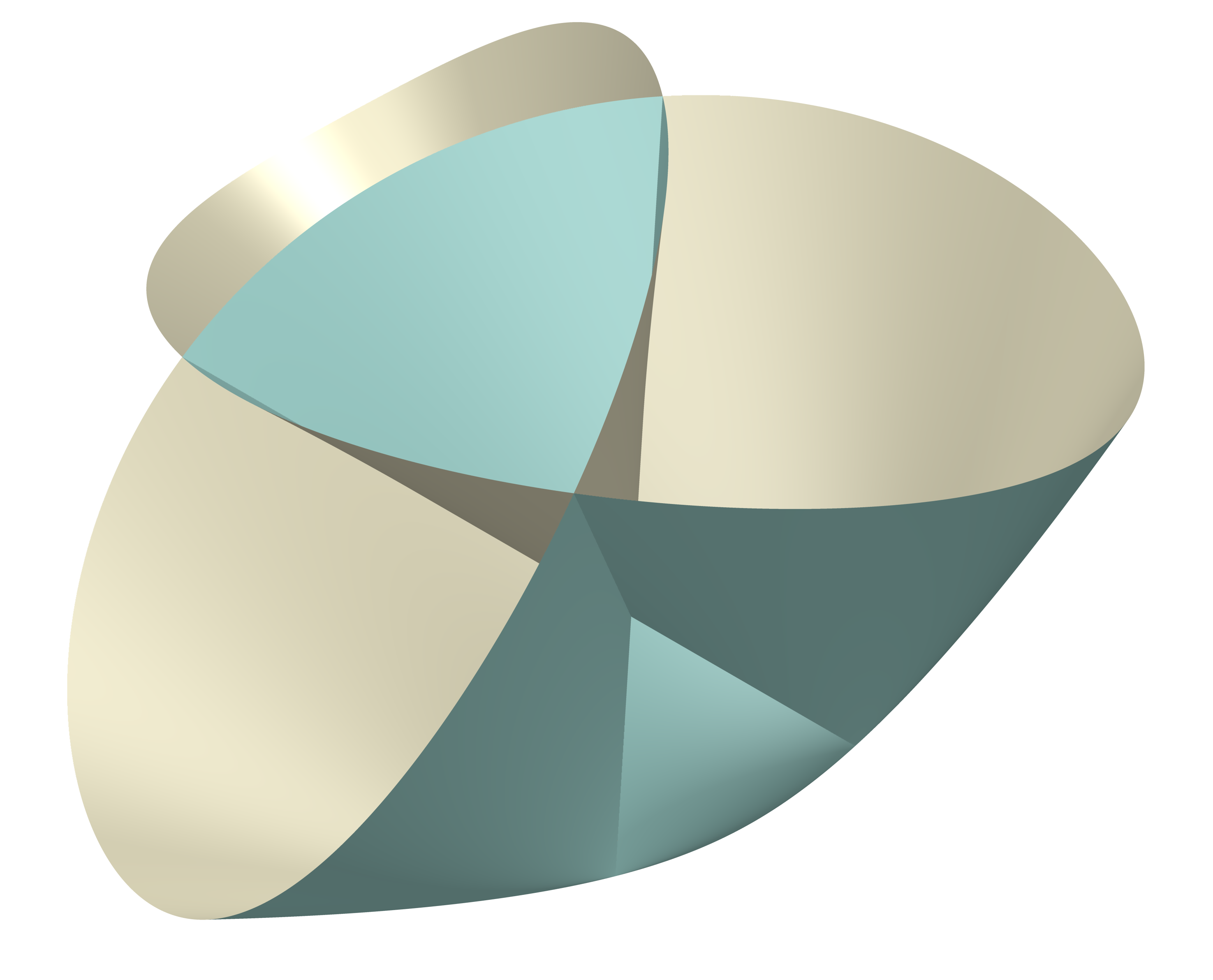
Figure 3.1. The coordinate-wise square of the plane $V(x_{0}+x_{1}+x_{2}+x_{3})\subset\mathbb{P}^{3}$.

This rational quartic surface is illustrated in Figure 3.1. It is a Steiner surface with three singular lines forming the ramification locus of ${\mathopen{}\mathclose{{}\left.\kern-1.2pt\varphi_{2}}\right|_{V(f)}}\colon V(f)\to V(f)^{\circ 2}$.

Example 3.6 (Squaring the circle).

Consider the plane conic $C=V(f)\subset\mathbb{P}^{2}$ given by $f:=(x_{1}-ax_{0})^{2}+(x_{2}-bx_{0})^{2}-(cx_{0})^{2}$ for some $a,b,c\in\mathbb{R}$ with $c>0$. In the affine chart $x_{0}=1$, this corresponds over the real numbers to the circle with center $(a,b)$ and radius $c$. From 3.4, we show that the coordinate-wise square of the circle $C\subset\mathbb{P}^{2}$ can be a line, a parabola or a singular quartic curve. See Figure 3.2 for an illustration of the following three cases:

1. If the circle $C$ is centered at the origin (i.e. $a=b=0$), then $\operatorname{\mathfrak{s}}_{r}(f)=f$ and $C^{\circ 2}\subset\mathbb{P}^{2}$ is the line defined by the equation $f^{\circ 2}=x_{1}+x_{2}-c^{2}x_{0}.$

2. If the center of the circle lies on a coordinate-axis and is not the origin (i.e. $ab=0$, but $(a,b)\neq(0,0)$), then $C^{\circ 2}\subset\mathbb{P}^{2}$ is a conic. Say $a=0$, then $C^{\circ 2}$ is defined by the equation $f^{\circ 2}=(x_{1}+x_{2})^{2}+2(b^{2}-c^{2})x_{0}x_{1}-2(b^{2}+c^{2})x_{0}x_{2}+(b^{2}-c^{2})^{2}x_{0}^{2}.$ In the affine chart $x_{0}=1$, $C$ is a circle and $C^{\circ 2}$ is a parabola.

3. If the center of the circle does not lie on a coordinate-axis, then $|\mathcal{G}_{r}\cdot f|=4$. Therefore, $C^{\circ 2}$ is a quartic plane curve. Its equation can be computed explicitly using 3.4. Being the image of a conic, the quartic curve $C^{\circ 2}$ is rational, hence it cannot be smooth. In fact, its singularities are the two points $[0:1:-1]$ and $[a^{2}+b^{2}:b^{2}(c^{2}-a^{2}-b^{2}):a^{2}(c^{2}-a^{2}-b^{2})]$ in $\mathbb{P}^{2}$. They form the branch locus of ${\mathopen{}\mathclose{{}\left.\kern-1.2pt\varphi_{2}}\right|_{C}}\colon C\to C^{\circ 2}$. The point $[0:1:-1]\in\mathbb{P}^{2}$ is the image of the two complex points $[0:1:\pm i]$ at infinity lying on all of the four conics $\tau\cdot C$ for $\tau\in\mathcal{G}_{2}$. The other singular point of $C^{\circ 2}$ is the image under $\varphi_{2}$ of the two intersection points of the two circles $C$ and $\tau\cdot C$ for $\tau=[1:-1:-1]\in\mathcal{G}_{2}$ inside the affine chart $x_{0}=1.$

${\vbox{\hbox{\includegraphics[height=113.81102pt]{squaringcircles4.png}}}}\qquad\longrightarrow\qquad{\vbox{\hbox{\includegraphics[height=113.81102pt]{CirclesSquared.png}}}}$

Figure 3.2. Circles and their coordinate-wise squares

Remark 3.7 (Newton polytope of $f^{\circ r}$).

Let $f\in\mathbb{P}(\mathbb{C}[\mathbf{x}]_{d})$ be irreducible and $f\neq x_{i}$. Then the Newton polytope of $f^{\circ r}$ arises from the Newton polytope of $f$ by rescaling according to the cardinality of the orbit $\mathcal{G}_{r}\cdot f\subset\mathbb{P}(\mathbb{C}[\mathbf{x}]_{d})$:

$$\operatorname{Newt}(f^{\circ r})=\frac{|\mathcal{G}_{r}\cdot f|}{r}\cdot\operatorname{Newt}(f)\subset\mathbb{R}^{n+1}.$$

Indeed, we have $\operatorname{Newt}(\tau\cdot f)=\operatorname{Newt}(f)$ for all $\tau\in\mathcal{G}_{r}$, and since $\operatorname{Newt}(gh)=\operatorname{Newt}(g)+\operatorname{Newt}(h)$ holds for all polynomials $g,h$, we have $\operatorname{Newt}(\operatorname{\mathfrak{s}}_{r}(f))=|\mathcal{G}_{r}\cdot f|\cdot\operatorname{Newt}(f)$ by Definition 3.2. Replacing $x_{i}^{r}$ by $x_{i}$ rescales the Newton polytope with the factor $\frac{1}{r}$, so the claim follows.

3.2. Duals and reciprocals of power sum hypersurfaces

We now highlight the interactions between coordinate-wise powers, dual and reciprocal varieties for the case of power sum hypersurfaces $V(x_{0}^{p}+\ldots+x_{n}^{p})\subset\mathbb{P}^{n}$. Specifically, we determine explicitly all hypersurfaces that arise from power sum hypersurfaces by repeatedly taking duals and reciprocals as the coordinate-wise $r$-th power of some hypersurface. In this subsection, we also allow $r$ to take negative integer values.

Recall that the reciprocal variety $V(f)^{\circ(-1)}$ of a hypersurface $V(f)\subset\mathbb{P}^{n}$ not containing any coordinate hyperplane of $\mathbb{P}^{n}$ is defined as the closure of $\varphi_{-1}(V(f)\setminus V(x_{0}x_{1}\ldots x_{n}))$ in $\mathbb{P}^{n}$. We denote it also by $\operatorname{\mathcal{R}}V(f)$. For linear spaces the reciprocal variety and its Chow form has been studied in detail in [KV16].

We also recall the definition of the dual variety of $V(f)\subset\mathbb{P}^{n}$. Consider the set of hyperplanes in $\mathbb{P}^{n}$ that arise as the projective tangent space at a smooth point of $V(f)$. This is a subset of the dual projective space $(\mathbb{P}^{n})^{*}$ and its Zariski closure is the dual variety of $V(f)$, which we denote by $V(f)^{*}$ or $\operatorname{\mathcal{D}}V(f)$. We identify $(\mathbb{C}^{n+1})^{*}$ with $\mathbb{C}^{n+1}$ via the standard bilinear form and therefore identify $(\mathbb{P}^{n})^{*}$ with $\mathbb{P}^{n}$.

Consider the power sum polynomial $\mathfrak{f}_{p}:=x_{0}^{p}+\ldots+x_{n}^{p}\in\mathbb{P}(\mathbb{C}[\mathbf{x}]_{p})$ for $p\in\mathbb{N}$. As before, we regard polynomials only up to scaling. For power sums with negative exponents we consider the numerator of the rational function as

$$\mathfrak{f}_{-p}:=(x_{1}x_{2}x_{3}\ldots x_{n})^{p}+(x_{0}x_{2}x_{3}\ldots x_{n})^{p}+\ldots+(x_{0}x_{1}x_{2}\ldots x_{n-1})^{p}\in\mathbb{P}(\mathbb{C}[\mathbf{x}]_{np})\quad\text{for }p\in\mathbb{N}.$$

In particular, $\mathfrak{f}_{-1}\in\mathbb{P}(\mathbb{C}[\mathbf{x}]_{n})$ is the elementary symmetric polynomial of degree $n$.

Recall that the morphism $\varphi_{r}\colon\mathbb{P}^{n}\to\mathbb{P}^{n}$ for $r>0$ is finite, hence preserves dimension. Since $\varphi_{-1}\colon\mathbb{P}^{n}\dashrightarrow\mathbb{P}^{n}$ is a birational map, the rational map $\varphi_{-r}=\varphi_{-1}\circ\varphi_{r}$ also preserves dimensions: $\dim V(\mathfrak{f}_{p})^{\circ(-r)}=\dim V(\mathfrak{f}_{p})$. We therefore extend Definition 3.1 to include the defining equation of $V(\mathfrak{f}_{p})^{\circ r}$ by $\mathfrak{f}_{p}^{\circ r}$ for all $p,r\in\mathbb{Z}\setminus\{0\}$. For the constant polynomial $\mathfrak{f}_{0}=1\in\mathbb{P}(\mathbb{C}[\mathbf{x}]_{0})$, we define $\mathfrak{f}_{0}^{\circ r}:=1$ for all $r\in\mathbb{Z}\setminus\{0\}$.

Lemma 3.8.

For all $s\in\mathbb{Z}$ and $r,\lambda\in\mathbb{Z}\setminus\{0\}$, we have $\mathfrak{f}_{\lambda s}^{\circ(\lambda r)}=\mathfrak{f}_{s}^{\circ r}$.

Proof.

For $\lambda>0$, we have $\varphi_{\lambda}^{-1}(V(\mathfrak{f}_{s}))=V(\mathfrak{f}_{\lambda s})$, hence

$$V(\mathfrak{f}_{\lambda s}^{\circ(\lambda r)})=\varphi_{r}(\varphi_{\lambda}(V(\mathfrak{f}_{\lambda s})))=\varphi_{r}(V(\mathfrak{f}_{s}))=V(\mathfrak{f}_{s}^{\circ r}),$$

where we have used the surjectivity of $\varphi_{\lambda}\colon\mathbb{P}^{n}\to\mathbb{P}^{n}$. For $\lambda<0$, we use the above to see

$$V(\mathfrak{f}_{\lambda s}^{\circ(\lambda r)})=(V(\mathfrak{f}_{\lambda s})^{\circ(-\lambda)})^{\circ(-r)}=V(\mathfrak{f}_{-s})^{\circ(-r)}=(\operatorname{\mathcal{R}}V(\mathfrak{f}_{-s}))^{\circ r}.$$

The reciprocal variety of $V(\mathfrak{f}_{-s})$ is $V(\mathfrak{f}_{s})$ for all $s\in\mathbb{Z}$. Hence, $V(\mathfrak{f}_{\lambda s}^{\circ(\lambda r)})=V(\mathfrak{f}_{s})^{\circ r}$. ∎

This naturally leads us to the our next definition.

Definition 3.9 (Generalised power sum polynomial).

For any rational number $p=\frac{s}{r}\in\mathbb{Q}$ ($r,s\in\mathbb{Z}$, $r\neq 0$), we define the generalised power sum polynomial $\mathfrak{f}_{p}:=\mathfrak{f}_{s}^{\circ r}\in\mathbb{P}(\mathbb{C}[\mathbf{x}]_{d})$.

By Lemma 3.8, the generalised power sum polynomial $\mathfrak{f}_{p}$ is well-defined. With this definition, we get the following duality result for hypersurfaces generalising Example 4.16 in [GKZ94].

Proposition 3.10 (Duality of generalised power sum hypersurfaces).

Let $p,q\in\mathbb{Q}\setminus\{0\}$ be such that $\frac{1}{p}+\frac{1}{q}=1$. Then $V(\mathfrak{f}_{p})^{*}=V(\mathfrak{f}_{q})$.

Proof.

Write $p=\frac{s}{r}$ with $r\in\mathbb{Z}\setminus\{0\}$, $s\in\mathbb{Z}_{>0}$. Let $b\in V(\mathfrak{f}_{p})=\varphi_{r}(V(\mathfrak{f}_{s}))$ be a smooth point of $V(\mathfrak{f}_{p})\setminus V(x_{0}x_{1}\ldots x_{n})$, and let $a\in V(\mathfrak{f}_{s})\setminus V(x_{0}x_{1}\ldots x_{n})$ be such that $b=\varphi_{r}(a)$. The morphism $\varphi_{r}\colon\mathbb{P}^{n}\setminus V(x_{0}x_{1}\ldots x_{n})\to\mathbb{P}^{n}\setminus V(x_{0}x_{1}\ldots x_{n})$ induces a linear isomorphism on projective tangent spaces $\mathbb{T}_{a}\mathbb{P}^{n}=\mathbb{P}^{n}\to\mathbb{P}^{n}=\mathbb{T}_{b}\mathbb{P}^{n}$ given by $\operatorname{diag}(ra_{0}^{r-1},ra_{1}^{r-1},\ldots,ra_{n}^{r-1})$. This maps

$$\mathbb{T}_{a}V(\mathfrak{f}_{s})=V\mathopen{}\mathclose{{}\left(\sum_{i=0}^{n}(\partial_{i}\mathfrak{f}_{s})(a)\>x_{i}}\right)\subset\mathbb{P}^{n}\quad\text{onto}\quad\mathbb{T}_{b}V(\mathfrak{f}_{p})=V\mathopen{}\mathclose{{}\left(\sum_{i=0}^{n}\frac{(\partial_{i}\mathfrak{f}_{s})(a)}{ra_{i}^{r-1}}\>x_{i}}\right)\subset\mathbb{P}^{n}.$$

In particular, $V(\mathfrak{f}_{p})^{*}\subset\mathbb{P}^{n}$ is the image of the rational map

$$V(\mathfrak{f}_{s})\dashrightarrow\mathbb{P}^{n},\qquad x\mapsto\mathopen{}\mathclose{{}\left[\frac{\partial_{0}\mathfrak{f}_{s}}{rx_{0}^{r-1}}:\frac{\partial_{1}\mathfrak{f}_{s}}{rx_{1}^{r-1}}:\ldots:\frac{\partial_{n}\mathfrak{f}_{s}}{rx_{n}^{r-1}}}\right].$$

From $\partial_{i}\mathfrak{f}_{s}=sx_{i}^{s-1}$ we conclude that $V(\mathfrak{f}_{p})^{*}=\varphi_{s-r}(V(\mathfrak{f}_{s}))=V(\mathfrak{f}_{s/(s-r)})=V(\mathfrak{f}_{q})$. ∎

Remark 3.11.

This statement can be understood as an algebraic analogue of the duality theory for $\ell^{p}$-spaces $(\mathbb{R}^{n},|\cdot|_{p})$. Indeed, let $p,q\geq 1$ be rational with $\frac{1}{p}+\frac{1}{q}=1$. The unit ball in $(\mathbb{R}^{n},|\cdot|_{p})$ is $U_{p}:=\{v\in\mathbb{R}^{n}\mid\sum_{i}v_{i}^{p}=1\}$ and, by $\ell_{p}$-duality, hyperplanes tangent to $U_{p}$ correspond to the points on the unit ball $U_{q}$ of the dual normed vector space $(\mathbb{R}^{n},|\cdot|_{q})$. The complex projective analogues of the unit balls $U_{p}\subset\mathbb{R}^{n}$ are the generalised power sum hypersurfaces $V(\mathfrak{f}_{p})\subset\mathbb{P}^{n}$ and 3.10 shows the previous statement in this setting.

Using 3.4 we can compute $\mathfrak{f}_{p}$ for any $p\in\mathbb{Q}$ explicitly. In particular, we make the following observation:

Lemma 3.12.

Let $s\in\mathbb{N}$ and $r\in\mathbb{Z}\setminus\{0\}$ be relatively prime. Then $\mathfrak{f}_{s/r}$ arises from $\mathfrak{f}_{1/r}$ by substituting $x_{i}\mapsto x_{i}^{s}$ for all $i\in\{0,1,\ldots,n\}$.

Proof.

This follows from the explicit description of the polynomials $\mathfrak{f}_{s/r}=\mathfrak{f}_{s}^{\circ r}$ and $\mathfrak{f}_{1/r}=\mathfrak{f}_{1}^{\circ r}$ given by 3.4. ∎

By Lemma 3.12, in order to determine the generalised power sum polynomials $\mathfrak{f}_{p}$, we may restrict our attention to $\mathfrak{f}_{1/r}$. These have a particular geometric interpretation as repeated dual-reciprocals of the linear space $V(x_{0}+x_{1}+\ldots+x_{n})\subset\mathbb{P}^{n}$ as in 3.14.

Theorem 3.13.

The repeated dual-reciprocals of generalised power sum hypersurfaces $V(\mathfrak{f}_{p})$ are given by

$$(\operatorname{\mathcal{D}}\operatorname{\mathcal{R}})^{k}\>V(\mathfrak{f}_{p}) =V(\mathfrak{f}_{p/(1+kp)})\qquad\forall k\in\mathbb{N},\;p\in\mathbb{Q}\setminus\{0,-\frac{1}{k},-\frac{1}{k-1},\ldots,-1\}\quad\text{and}$$

$$(\operatorname{\mathcal{R}}\operatorname{\mathcal{D}})^{k}\>V(\mathfrak{f}_{p}) =V(\mathfrak{f}_{p/(1-kp)})\qquad\forall k\in\mathbb{N},\;p\in\mathbb{Q}\setminus\{0,\frac{1}{k},\frac{1}{k-1},\ldots,1\}.$$

Proof.

We show the claim for $V(\mathfrak{f}_{p})$ by induction on $k$. For $k=0$, the claim is trivial. For $k>0$, we get by induction hypothesis:

$$(\operatorname{\mathcal{D}}\operatorname{\mathcal{R}})^{k}\>V(\mathfrak{f}_{p}) =\operatorname{\mathcal{D}}\operatorname{\mathcal{R}}V(\mathfrak{f}_{p/(1+(k-1)p)})=(V(\mathfrak{f}_{p/(1+(k-1)p)})^{\circ(-1)})^{*}$$

$$\stackrel{{\scriptstyle(*)}}{{=}}V(\mathfrak{f}_{-p/(1+(k-1)p)})^{*}\stackrel{{\scriptstyle(**)}}{{=}}V(\mathfrak{f}_{p/(1+kp)}),$$

where $(*)$ holds by Lemma 3.8 and $(**)$ by 3.10. From this, we also see

$$(\operatorname{\mathcal{R}}\operatorname{\mathcal{D}})^{k}\>V(\mathfrak{f}_{p})=\operatorname{\mathcal{R}}(\operatorname{\mathcal{D}}\operatorname{\mathcal{R}})^{k}\operatorname{\mathcal{R}}V(\mathfrak{f}_{p})=\operatorname{\mathcal{R}}(\operatorname{\mathcal{D}}\operatorname{\mathcal{R}})^{k}V(\mathfrak{f}_{-p})=\operatorname{\mathcal{R}}V(\mathfrak{f}_{-p/(1-kp)})=V(\mathfrak{f}_{p/(1-kp)}),$$

concluding the proof. ∎

Corollary 3.14.

For $r>0$, the repeated alternating reciprocals and duals of the linear space $V(\mathfrak{f}_{1})\subset\mathbb{P}^{n}$ are the coordinate-wise powers of $V(\mathfrak{f}_{1})$ given as

$${\underbrace{\operatorname{\mathcal{D}}\operatorname{\mathcal{R}}\operatorname{\mathcal{D}}\operatorname{\mathcal{R}}\ldots\operatorname{\mathcal{D}}\operatorname{\mathcal{R}}}_{2r-2}}\>V(\mathfrak{f}_{1}) =V(\mathfrak{f}_{1})^{\circ r}\qquad\text{and}\qquad{\underbrace{\operatorname{\mathcal{R}}\operatorname{\mathcal{D}}\operatorname{\mathcal{R}}\ldots\operatorname{\mathcal{D}}\operatorname{\mathcal{R}}}_{2r-1}}\>V(\mathfrak{f}_{1})=V(\mathfrak{f}_{1})^{\circ(-r)}.$$

Example 3.15.

Let $n=3$ and $f:=x_{0}+x_{1}+x_{2}+x_{3}$. The reciprocal variety of the plane $V(f)\subset\mathbb{P}^{3}$ is given by $\mathfrak{f}_{-1}=x_{1}x_{2}x_{3}+x_{0}x_{2}x_{3}+x_{0}x_{1}x_{3}+x_{0}x_{1}x_{2}$. Its dual is $V(\mathfrak{f}_{1/2})=V(\mathfrak{f}_{1})^{\circ 2}\subset\mathbb{P}^{3}$ by 3.10. This is the quartic surface from Example 3.5. Higher iterated dual-reciprocal varieties of $V(f)$ can be explicitly computed analogous to Example 3.5 via 3.13. For instance, the surface $\operatorname{\mathcal{D}}\operatorname{\mathcal{R}}\operatorname{\mathcal{D}}\operatorname{\mathcal{R}}V(f)\subset\mathbb{P}^{3}$ is the coordinate-wise cube of $V(f)$ which is the degree 9 surface illustrated in Figure 3.3.

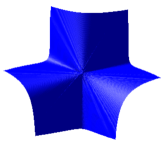
Figure 3.3. The iterated dual-reciprocal $\operatorname{\mathcal{D}}\operatorname{\mathcal{R}}\operatorname{\mathcal{D}}\operatorname{\mathcal{R}}V(f)\subset\mathbb{P}^{3}$

Remark 3.16 (Coordinate-wise rational powers).

The construction of the generalised power sum hypersurfaces $V(\mathfrak{f}_{p})$ may be understood in a broader context of coordinate-wise powers with rational exponents: For a subvariety $X\subset\mathbb{P}^{n}$, and a rational number $p=r/s$ with $r\in\mathbb{Z}$ and $s\in\mathbb{Z}_{>0}$ relatively prime, we may define the coordinate-wise $p$-th power $X^{\circ p}:=\varphi_{s}^{-1}(X^{\circ r})=(\varphi_{s}^{-1}(X))^{\circ r}$. This is a natural generalisation of the coordinate-wise integer powers $X^{\circ r}$. With this definition, the generalised power sum hypersurface $V(\mathfrak{f}_{p})$ is the $1/p$-th coordinate-wise power of $V(\mathfrak{f}_{1})$. While we focus on coordinate-wise powers to integral exponents in this article, many results easily transfer to the case of rational exponents. For instance, the defining ideal of $X^{\circ(r/s)}$ is obtained by substituting $x_{i}\mapsto x_{i}^{s}$ in each of the generators of the vanishing ideal of $X^{\circ r}$ – in particular, the number of minimal generators for these two ideals agree.

3.3. From hypersurfaces to arbitrary varieties?

We briefly discuss to what extent 3.4 can be used to determine coordinate-wise powers of arbitrary varieties, and mention the difficulties involved in this approach.

Let $r>0$ and let $f_{1},\ldots,f_{m}$ be homogeneous polynomials vanishing on a variety $X\subset\mathbb{P}^{n}$. Their $r-$th coordinate-wise powers give rise to the inclusion $X^{\circ r}\subset V(f_{1}^{\circ r},\ldots,f_{m}^{\circ r})$. We may ask when equality holds, which leads us to the following definition, reminiscent of the notion of tropical bases in Tropical Geometry [MS15, Section 2.6].

Definition 3.17 (Power basis).

A set of homogeneous polynomials $f_{1},\ldots,f_{m}\subset\mathbb{C}[\mathbf{x}]$ is an $r$-th power basis of the ideal $I=(f_{1},\ldots,f_{m})$ if the following equality of sets holds:

$$V(f_{1},\ldots,f_{m})^{\circ r}=V(f_{1}^{\circ r},\ldots,f_{m}^{\circ r}).$$

We show the existence of such power bases for a given ideal in the following proposition.

Proposition 3.18 (Existence of power bases).

Let $I\subset\mathbb{C}[\mathbf{x}]$ be a homogeneous ideal. Then for each $r$, there exists an $r$-th power basis of $I$.

Proof.

Let $J$ denote the defining ideal of $V(I)^{\circ r}\subset\mathbb{P}^{n}$. If $J$ is generated by homogeneous polynomials $g_{1},\ldots,g_{m}\in\mathbb{C}[\mathbf{x}]$, we define $f_{1},\ldots,f_{m}\in\mathbb{C}[\mathbf{x}]$ to be their images under the ring homomorphism $\mathbb{C}[\mathbf{x}]\to\mathbb{C}[\mathbf{x}]$, $x_{i}\mapsto x_{i}^{r}$. Then $f_{i}\in I$, since

$$V(f_{i})=\varphi_{r}^{-1}(V(g_{i}))\supset\varphi_{r}^{-1}(V(I)^{\circ r})\supset V(I).$$

On the other hand, we have $f_{i}^{\circ r}=g_{i}$, since $V(f_{i})^{\circ r}=\varphi_{r}(\varphi_{r}^{-1}(V(g_{i})))=V(g_{i})$ by surjectivity of $\varphi_{r}$. Therefore, $f_{1}^{\circ r},\ldots,f_{m}^{\circ r}$ generate $J$. Enlarging $f_{1},\ldots,f_{m}$ to a generating set of $I$ gives an $r$-th power basis of $I$. ∎

Remark 3.19.

3.18 shows the existence of $r$-th power bases, but explicitly determining one a priori is nontrivial. For the variety of orthostochastic matrices $\mathbb{O}(m)^{\circ 2}$ as in Section 2.1, it is natural to suspect that the quadratic equations defining the variety of orthogonal matrices would form a power basis for $r=2$. This is the question discussed in [CĐ08, Section 3], where it was shown that this is true for $m=3$, but not for $m\geq 6$. The cases $m=4,5$ are an open problem [CĐ08, Problem 6.2]. Our results on the degree of $\mathbb{O}(m)^{\circ 2}$ reduce this open problem to the computation whether explicitly given polynomials $f_{1}^{\circ 2},\ldots,f_{k}^{\circ 2}$ describe an irreducible variety of the correct dimension and degree. Straightforward implementations of this computation seem to be beyond current computer algebra software.

In the following two examples, we will see that even in the case of squaring codimension 2 linear spaces, obvious candidates for $f_{1},\ldots,f_{m}$ do not form a power basis.

Example 3.20.

Let $I:=(f_{1},f_{2})\subset\mathbb{C}[\mathbf{x}]$ be the ideal defining the line in $\mathbb{P}^{3}$ that is given by $f_{1}:=x_{0}+x_{1}+x_{2}+x_{3}$ and $f_{2}:=x_{1}+2x_{2}+3x_{3}$. The polynomials $f_{1}^{\circ 2}$ and $f_{2}^{\circ 2}$ have degrees 4 and 2, respectively, by 3.4. Note that the polynomial $f_{3}:=3x_{0}^{2}-x_{1}^{2}+x_{2}^{2}-3x_{3}^{2}=3(x_{0}-x_{1}-x_{2}-x_{3})f_{1}+2(x_{1}+x_{2})f_{2}$ also lies in $I$, so the ideal of $V(I)^{\circ 2}$ contains the linear form $f_{3}^{\circ 2}=3x_{0}-x_{1}+x_{2}-3x_{3}$. The polynomials $f_{1},f_{2}$ do not form a power basis of $I$. In fact, one can check that $V(f_{1}^{\circ 2},f_{2}^{\circ 2})\subset\mathbb{P}^{3}$ is the union of four rational quadratic curves, one of which is $V(I)^{\circ 2}$, see Figure 3.4 for an illustration. A power basis of $I$ is given by $f_{1},f_{2},f_{3}$.

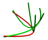
Figure 3.4. Distinction between $V(f_{1}^{\circ 2},f_{2}^{\circ 2})$ and $V(f_{1},f_{2})^{\circ 2}$

Example 3.21.

Another natural choice for polynomials $f_{1},\ldots,f_{m}$ in the ideal of a linear space $X\subset\mathbb{P}^{n}$ consists of the circuit forms, i.e. linear forms vanishing on $X$ that are minimal with respect to the set of occurring variables. However, for

$$X:=V(x_{0}+x_{1}+x_{2}+x_{3}+x_{4},\;x_{1}+2x_{2}+3x_{3}+4x_{4})\subset\mathbb{P}^{4},$$

these circuit forms are

$$f_{1}=x_{1}+2x_{2}+3x_{3}+4x_{4},\quad f_{2}=x_{0}-x_{2}-2x_{3}-3x_{4},\quad f_{3}=2x_{0}+x_{1}-x_{3}-2x_{4},$$

$$f_{4}=3x_{0}+2x_{1}+x_{2}-x_{4},\quad f_{5}=4x_{0}+3x_{1}+2x_{2}+x_{3},$$

and one can check that the point $[16:16:1:36:9]\in\mathbb{P}^{4}$ lies in $V(f_{1}^{\circ 2},\ldots,f_{5}^{\circ 2})$, but not in $X^{\circ 2}$. In particular, $f_{1},\ldots,f_{5}$ is not an $r$-th power basis for $r=2$.

We have seen in 3.20 and 3.21 that even for the case of linear spaces of codimension 2 it is not an easy task to a priori identify an $r$-th power basis.

The following proposition shows how one can straightforwardly find a very large $r$-th power basis of an ideal $I$, without first computing the ideal of $V(I)^{\circ r}$.

Proposition 3.22.

If $g_{1},\ldots,g_{k}\in\mathbb{C}[\mathbf{x}]_{d}$ are forms of degree $d$, then taking $(k-1)r^{n}+1$ general linear combinations of $g_{1},\ldots,g_{k}$ produces an $r$-th power basis of $(g_{1},\ldots,g_{k})$.

Proof.

We assume that $g_{1},\ldots,g_{k}$ are linearly independent, or else we can replace them with a linearly independent subset. For $m:=(k-1)r^{n}+1$, let $f_{1},\ldots,f_{m}\in\langle g_{1},\ldots,g_{k}\rangle$ be such that no $k$ of them are linearly dependent. For $X:=V(g_{1},\ldots,g_{k})$, we will show that $V(f_{1}^{\circ r},\ldots,f_{m}^{\circ r})=X^{\circ r}$ by comparing the preimages of both sides under $\varphi_{r}\colon\mathbb{P}^{n}\to\mathbb{P}^{n}$.

By Proposition 2.1, we have $\varphi_{r}^{-1}(X^{\circ r})=\bigcup_{\tau\in\mathcal{G}_{r}}\tau\cdot X$ and

$$\varphi_{r}^{-1}(V(f_{1}^{\circ r},\ldots,f_{m}^{\circ r}))=\bigcap_{i=1}^{m}\varphi_{r}^{-1}(\varphi_{r}(V(f_{i})))=\bigcap_{i=1}^{m}\bigcup_{\tau\in\mathcal{G}_{r}}\tau\cdot V(f_{i}).$$

Let $p\in\varphi_{r}^{-1}(V(f_{1}^{\circ r},\ldots,f_{m}^{\circ r}))\subset\mathbb{P}^{n}$. Then for each $i\in\{1,\ldots,m\}$ there exists some $\tau\in\mathcal{G}_{r}$ with $p\in\tau\cdot V(f_{i})$ using the last equality above. Since $m>(k-1)|\mathcal{G}_{r}|$, by pigeonhole principle there must exist $\tau\in\mathcal{G}_{r}$ and $i_{1},i_{2},\ldots,i_{k}\in\{1,\ldots,m\}$ distinct with $p\in\bigcap_{j=1}^{k}\tau\cdot V(f_{i_{j}})=\tau\cdot V(f_{i_{1}},\ldots,f_{i_{k}})$. Since, by assumption, no $k$ of them are linearly dependent $f_{i_{1}},\ldots,f_{i_{k}}$ span $\langle g_{1},\ldots,g_{k}\rangle$. Therefore, $V(f_{i_{1}},\ldots,f_{i_{k}})=X$, and hence, $p\in\tau\cdot V(f_{i_{1}},\ldots,f_{i_{k}})$ implies that $p\in\tau\cdot X\subset\varphi_{r}^{-1}(X^{\circ r})$. This shows $\varphi_{r}^{-1}(V(f_{1}^{\circ r},\ldots,f_{m}^{\circ r}))\subset\varphi_{r}^{-1}(X)$. The reverse inclusion is trivial. ∎

In particular, 3.22 shows that for a subvariety of $\mathbb{P}^{n}$ defined by $k$ forms of degree $d$, its coordinate-wise $r$-th power can be described set-theoretically by the vanishing of $(k-1)r^{n}+1$ forms of degree $\leq dr^{n-1}$. However, we will see in Section 4 that for linear spaces this bound is rather weak in many cases and should be expected to allow dramatic refinement in general. We raise the following as a broad open question:

Question 3.23.

When does a set of homogeneous polynomials form an $r$-th power basis? For a given ideal $I$, do there exist polynomials $f_{1},\ldots,f_{m}\in I$ that simultaneously form an $r$-th power basis for all $r$?

4. Linear spaces

In this section, we specialise to linear spaces $L\subset\mathbb{P}^{n}$ and investigate their coordinate-wise powers $L^{\circ r}$. First, we highlight the dependence of $L^{\circ r}$ on the geometry of a finite point configuration associated to $L\subset\mathbb{P}^{n}$. For $r=2$, we point out its relation to symmetric matrices with degenerate eigenvalues. Based on this, we classify the coordinate-wise squares of lines and planes. Finally, we turn to the case of squaring linear spaces in high-dimensional ambient space.

4.1. Point configurations

We study the defining ideal of $L^{\circ r}$ for a $k$-dimensional linear space $L\subset\mathbb{P}^{n}$. The degrees of its minimal generators do not change under rescaling and permuting coordinates of $\mathbb{P}^{n}$, i.e. under the actions of the algebraic torus $\mathbb{G}_{m}^{n+1}=(\mathbb{C}^{*})^{n+1}$ and the symmetric group $\mathfrak{S}_{n+1}$. Fixing a $(k+1)$-dimensional vector space $W$, we have the identification

$$\{\text{\small orbits of $\operatorname{Gr}(k,\mathbb{P}^{n})$ under $\mathbb{G}_{m}^{n+1}\rtimes\mathfrak{S}_{n+1}$}\} \leftrightarrow\mathopen{}\mathclose{{}\left\{\begin{subarray}{c}\text{\small finite multi-sets $Z\subset\mathbb{P}W^{*}$ with $\langle Z\rangle=\mathbb{P}W^{*}$}\\ \text{\small of cardinality $\leq n+1$ up to $\operatorname{Aut}(\mathbb{P}W^{*})$}\end{subarray}}\right\}$$

$$L=\operatorname{im}(\mathbb{P}W\xhookrightarrow{[\ell_{0}:\ell_{1}:\ldots:\ell_{s}:0:\ldots:0]}\mathbb{P}^{n}) \begin{subarray}{c}\mapsfrom\\ \mapsto\end{subarray}\qquad Z=\{[\ell_{0}],[\ell_{1}],\ldots,[\ell_{s}]\}\subset\mathbb{P}W^{*},s\leq n.$$

Hence, we may express coordinate-wise powers of a linear space $L$ in terms of the corresponding finite multi-set $Z\subset\mathbb{P}W^{*}$. In fact, it is easy to check that the degrees of the minimal generators of the defining ideal only depend on the underlying set $Z$, forgetting repetitions in the multi-set. We study coordinate-wise powers of a linear space in terms of the corresponding non-degenerate finite point configuration.

For the entirety of Section 4, we establish the following notation: Let $L\subset\mathbb{P}^{n}$ be a linear space of dimension $k$. We understand $L$ as the image of a chosen linear embedding $\iota\colon\mathbb{P}W\xhookrightarrow{[\ell_{0}:\ldots:\ell_{n}]}\mathbb{P}^{n}$, where $W$ is a $(k+1)$-dimensional vector space and $\ell_{0},\ldots,\ell_{n}\in W^{*}$ are linear forms defining $\iota$. Consider the finite set of points $Z\subset\mathbb{P}W^{*}$ given by

$$Z:=\{[\ell_{i}]\in\mathbb{P}W^{*}\mid 0\leq i\leq n\text{ such that }\ell_{i}\neq 0\}.$$

Since $\ell_{0},\ell_{1},\ldots,\ell_{n}\in W^{*}$ define the linear embedding $\iota$, they cannot have a common zero in $W$. Hence, the linear span of $Z$ is the whole space $\mathbb{P}W^{*}$. We denote by $I(Z)\subset\operatorname{Sym}^{\bullet}W$ the defining ideal of $Z\subset\mathbb{P}W^{*}$. The subspace of degree $r$ forms vanishing on $Z$ is written as $I(Z)_{r}\subset\operatorname{Sym}^{r}W$.

The main technical tool is the following observation that $L^{\circ r}\subset\mathbb{P}^{n}$ equals (up to a linear re-embedding) the image of the $r$-th Veronese variety $\nu_{r}(\mathbb{P}W)\subset\mathbb{P}\operatorname{Sym}^{r}W$ under the projection from the linear space $\mathbb{P}(I(Z)_{r})\subset\mathbb{P}\operatorname{Sym}^{r}W$.

Lemma 4.1.

The diagram

commutes, where $\nu_{r}$ is the $r$-th Veronese embedding, $\pi$ is the linear projection of $\mathbb{P}\operatorname{Sym}^{r}W$ from the linear space $\mathbb{P}(I(Z)_{r})$, $\psi$ is a morphism and $\vartheta$ is a linear embedding.

Proof.

We observe that the morphism $\varphi_{r}\circ\iota$ is given by

$$\varphi_{r}\circ\iota\colon\mathbb{P}W\to\mathbb{P}^{n},\qquad[v]\mapsto[\ell_{0}^{r}(v):\ell_{1}^{r}(v)\ldots:\ell_{n}^{r}(v)].$$

The $n+1$ elements $\ell_{i}^{r}\in\operatorname{Sym}^{r}W^{*}$ correspond to a linear map $\chi\colon\operatorname{Sym}^{r}W\to\mathbb{C}^{n+1}$ via the natural identification $(\operatorname{Sym}^{r}W^{*})^{n+1}=\operatorname{Hom}_{\mathbb{C}}(\operatorname{Sym}^{r}W,\mathbb{C}^{n+1})$.

The rational map $\bar{\chi}$ between projective spaces corresponding to the linear map $\chi$ gives the following commuting diagram:

where $\vartheta$ is the linear embedding of projective spaces induced by factoring $\chi$ over $\operatorname{Sym}^{r}W/\ker\chi$. In particular, $\nu_{r}(\mathbb{P}W)\cap\mathbb{P}(\ker\chi)=\emptyset$, since $\varphi_{r}\circ\iota$ is defined everywhere on $\mathbb{P}W$. Hence, ${\mathopen{}\mathclose{{}\left.\kern-1.2pt\pi}\right|_{\nu_{r}(\mathbb{P}W)}}\colon\nu_{r}(\mathbb{P}W)\to\mathbb{P}(\operatorname{Sym}^{r}W/\ker\chi)$ is a morphism.

Finally, we claim that $\ker\chi=I(Z)_{r}$. Once we know this, defining $\psi:={\mathopen{}\mathclose{{}\left.\kern-1.2pt\pi}\right|_{\nu_{r}(\mathbb{P}W)}}\circ\nu_{r}$ completes the claimed diagram.

Let $f\in\operatorname{Sym}^{r}W$ such that $f\in I(Z)_{r}$. Naturally identifying $W$ and $W^{**}$, we may view $f$ as a form of degree $r$ on $W^{*}$. Then, the condition that $f\in I(Z)_{r}$ translates to $f(\ell_{i})=0\ \forall i$. Viewing $f$ as a symmetric $r$-linear form $W^{*}\times\ldots\times W^{*}\to\mathbb{C}$, we have $f(\ell_{i},\ldots,\ell_{i})=0\ \forall i$. Also, when $f$ is considered as a linear form on $\operatorname{Sym}^{r}W^{*}$, $f(\ell_{i}^{r})=0\ \forall i$. The latter expression is equivalent to $f\in\ker\chi$, via the identification of $W$ and $W^{**}$. We conclude $I(Z)_{r}=\ker\chi$. ∎

In particular, we deduce the following:

Proposition 4.2.

Let $L$ be a linear space such that the finite set of points $Z$ does not lie on a degree $r$ hypersurface. Then the ideal of $L^{\circ r}$ is generated by linear and quadratic forms.

Proof.

Since $I(Z)_{r}=0$, we deduce from Lemma 4.1 that $L^{\circ r}=\varphi_{r}(L)$ is a linear re-embedding of the $k$-dimensional $r$-th Veronese variety $\nu_{r}(\mathbb{P}W)\subset\mathbb{P}\operatorname{Sym}^{r}W$. The ideal of this Veronese variety is generated by quadrics. Since $\dim\operatorname{Sym}^{r}W=\tbinom{k+r}{r}$, the linear re-embedding $\vartheta\colon\mathbb{P}\operatorname{Sym}^{r}W\hookrightarrow\mathbb{P}^{n}$ adds $n-\smash{\binom{k+r}{r}}+1$ linear forms to the ideal. ∎

4.2. Degenerate eigenvalues and squaring

We now specialise to the case of coordinate-wise squaring, i.e. $r=2$. This case has special geometric importance, since it corresponds to computing the image of a linear space under the quotient of $\mathbb{P}^{n}$ by the reflection group generated by the coordinate hyperplanes. In this section through 4.3 we point out that the case of coordinate-wise square of a linear space is closely related to studying symmetric matrices with a degenerate spectrum of eigenvalues. Here, we interpret $\mathbb{P}\operatorname{Sym}^{2}\mathbb{F}^{k+1}$ (for $\mathbb{F}=\mathbb{R}$ or $\mathbb{C}$) as the projective space consisting of symmetric $(k+1)\times(k+1)$-matrices up to scaling with entries in $\mathbb{F}$.

Proposition 4.3.

Let $X\subset\mathbb{P}\operatorname{Sym}^{2}\mathbb{R}^{k+1}$ be the set of real symmetric $(k+1)\times(k+1)$-matrices with an eigenvalue of multiplicity $\geq k$. Then the Zariski closure of $X$ in $\mathbb{P}\operatorname{Sym}^{2}\mathbb{C}^{k+1}$ is projectively equivalent to the projective cone over the coordinate-wise square $L^{\circ 2}$ of any $k$-dimensional linear space $L$ whose point configuration $Z\subseteq\mathbb{P}W^{*}$ lies on a unique and smooth quadric.

Proof.

Let $L\subset\mathbb{P}^{n}$ be a $k$-dimensional linear space such that $I(Z)_{2}$ is spanned by a smooth quadric $q\in\mathbb{P}\operatorname{Sym}^{2}W$. Choosing coordinates of $W\cong\mathbb{C}^{k+1}$, we identify points in $\mathbb{P}\operatorname{Sym}^{2}W$ with complex symmetric $(k+1)\times(k+1)$-matrices up to scaling and we can assume $q=\operatorname{id}\in\mathbb{P}\operatorname{Sym}^{2}W$. The second Veronese variety $\nu_{2}(\mathbb{P}W)\subset\mathbb{P}\operatorname{Sym}^{2}W$ consists of rank $1$ matrices. Let $X_{0}\subset\mathbb{P}(\operatorname{Sym}^{2}W/\langle q\rangle)$ be the image of $\nu_{2}(\mathbb{P}W)$ under the natural projection. By Lemma 4.1, $X_{0}$ is the coordinate-wise square $L^{\circ 2}$ up to a linear re-embedding.

The projective cone over $X_{0}\cong L^{\circ 2}$ is the subvariety $X_{1}\subset\mathbb{P}\operatorname{Sym}^{2}W$ consisting of complex symmetric matrices $M$ such that the set $M+\langle\operatorname{id}\rangle$ contains a matrix of rank $\leq 1$. We observe that the rank of $M-\lambda\operatorname{id}$ is the codimension of the eigenspace of $M$ with respect to $\lambda\in\mathbb{C}$. Hence,

$$X_{1}=\{M\in\mathbb{P}\operatorname{Sym}^{2}\mathbb{C}^{k+1}\mid M\text{ has an eigenspace of codimension\leavevmode\nobreak\ $\leq 1$}\}.$$

We are left to show that $X_{1}$ is the Zariski closure in $\mathbb{P}\operatorname{Sym}^{2}\mathbb{C}^{k+1}$ of $X\subset\mathbb{P}\operatorname{Sym}^{2}\mathbb{R}^{k+1}$. Since real symmetric matrices are diagonalizable, the multiplicity of an eigenvalue is the dimension of the corresponding eigenspace. Hence, $X_{1}\cap\mathbb{P}\operatorname{Sym}^{2}\mathbb{R}^{k+1}=X$. The set $X$ is the orbit of the line $V:=\{\operatorname{diag}(\lambda,\ldots,\lambda,\mu)\mid[\lambda:\mu]\in\mathbb{P}_{\mathbb{R}}^{1}\}$ under the action of $O(k+1).$ The action is given by conjugation with orthogonal matrices and the stabiliser is $O(k)\times\{\pm 1\}$. Therefore, $X$ has real dimension $\dim V+\dim O(k+1)-\dim O(k)=k+1$. Also, $X_{1}$ is the projective cone over $X_{0}\cong L^{\circ 2}$, so it is a ${(k+1)}$-dimensional irreducible complex variety. We conclude that $X_{1}$ is the Zariski closure of $X$ in $\mathbb{P}\operatorname{Sym}^{2}\mathbb{C}^{k+1}$. ∎

We illustrate 4.3 in the case of $3\times 3$-matrices:

Example 4.4.

Consider the set of real symmetric $3\times 3$-matrices with a repeated eigenvalue. We denote its Zariski closure in $\mathbb{P}\operatorname{Sym}^{3}\mathbb{C}^{2}$ by $Y$. By 4.3, it can be understood in terms of the coordinate-wise square $L^{\circ 2}$ for some plane $L$. We make this explicit as follows: Consider the planar point configuration

$$Z=\{[1:i:0],[1:-i:0],[1:0:i],[1:0:-i],[0:1:i]\}\subseteq\mathbb{P}^{2},$$

lying only on the conic $V(x^{2}+y^{2}+z^{2})$. Let $L$ be the corresponding plane in $\mathbb{P}^{4}$, given as the image of

$$\iota\colon\mathbb{P}^{2}\hookrightarrow\mathbb{P}^{4},\qquad[x:y:z]\mapsto[x+iy:x-iy:x+iz:x-iz:y+iz].$$

Under the linear embedding

$$\psi\colon\mathbb{P}^{4} \hookrightarrow\mathbb{P}\operatorname{Sym}^{2}\mathbb{C}^{3},$$

$${\scriptsize[a:b:c:d:e]} \mapsto{\scriptsize\begin{bmatrix}2(a+b+c+d)&3i(-a+b)&3i(-c+d)\\ 3i(-a+b)&6(-2a-2b+c+d)&3i(-a-b+c+d-2e)\\ 3i(-c+d)&3i(-a-b+c+d-2e)&6(a+b-2c-2d),\end{bmatrix}},$$

the plane $L$ gets mapped into $Y$. Indeed, it is easily checked that a point $[x:y:z]$ gets mapped to the matrix $-4(x^{2}+y^{2}+z^{2})\operatorname{id}+12(x,y,z)^{T}(x,y,z)$ under the composition $\psi\circ\iota\colon\mathbb{P}^{2}\to\mathbb{P}\operatorname{Sym}^{2}\mathbb{C}^{3}$; note that this matrix has a repeated eigenvalue. More precisely, 4.3 shows that $Y$ is the projective cone over $\psi(L^{\circ 2})$ with the vertex $\operatorname{id}$.

In Section 4.4 we give an explicit set-theoretic description of the coordinate-wise square of a linear space in high-dimensional ambient space. We will show the following result as a special case of 4.11. Given a matrix $A\in\mathbb{C}^{s\times s}$, we denote a $2\times 2$ minor of $A$ by $A_{ij|k\ell}$ where $i,j$ are the rows and $k,\ell$ are the columns of the minor.

Corollary 4.5.

Let $s\geq 4$. A symmetric matrix $A\in\mathbb{C}^{s\times s}$ has an eigenspace of codimension $\leq 1$ if and only if its $2\times 2$-minors satisfy the following for $i,j,k,\ell\leq s$ distinct:

$$A_{ij|k\ell}=0,\qquad A_{ik|i\ell}=A_{jk|j\ell}\qquad\text{and}\qquad A_{ik|ik}-A_{i\ell|i\ell}=A_{jk|jk}-A_{j\ell|j\ell}.$$

These equations describe the Zariski closure in the complex vector space $\operatorname{Sym}^{2}\mathbb{C}^{s}$ of the set of real symmetric matrices with an eigenvalue of multiplicity $\geq s-1$.

4.3. Squaring lines and planes

In this subsection we consider the low-dimensional cases and classify the coordinate-wise squares of lines and planes in arbitrary ambient spaces.

Theorem 4.6 (Squaring lines).

Let $L$ be a line in $\mathbb{P}^{n}$.

1. If $|Z|=2$, then $L^{\circ 2}$ is a line in $\mathbb{P}^{n}$.

2. If $|Z|>2$, then $L^{\circ 2}$ is a smooth conic in $\mathbb{P}^{n}$.

Proof.

Since $Z\subset\mathbb{P}W^{*}$ spans the projective line $\mathbb{P}W^{*}$, we must have $|Z|\geq 2$.

If $|Z|>2$, then $I(Z)_{2}=0$, since no non-zero quadratic form on the projective line $\mathbb{P}W^{*}$ vanishes on all points of $Z$. Then Lemma 4.1 implies that $L^{\circ 2}=(\varphi_{2}\circ\iota)(\mathbb{P}W)$ is a linear re-embedding of $\nu_{2}(\mathbb{P}W)$, which is a smooth conic in the plane $\mathbb{P}\operatorname{Sym}^{2}W\cong\mathbb{P}^{2}$.

If $|Z|=2$, then $\dim I(Z)_{2}=1$, since up to scaling there is a unique quadric vanishing on the points $Z$. By Lemma 4.1, the image $\varphi_{2}(L)$ lies in a projective line $\mathbb{P}^{1}\cong\vartheta(\mathbb{P}(\operatorname{Sym}^{2}W/I(Z)_{2}))\subset\mathbb{P}^{n}$. On the other hand $\dim L^{\circ 2}=\dim L=1$. Hence, $L^{\circ 2}=\varphi_{2}(L)$ is a line in $\mathbb{P}^{n}$. ∎

Remark 4.7.

We observe that the two possibilities in 4.6 for the coordinate-wise square of a line $L$ differ in degree. In particular, 2.7 shows that it only depends on the linear matroid $\mathcal{M}_{L}$ whether $L^{\circ 2}$ is a line or a (re-embedded) plane conic.

Remark 4.8.

In the Grassmannian of lines $\operatorname{Gr}(1,\mathbb{P}^{n})$, consider the locus $\Gamma\subset\operatorname{Gr}(1,\mathbb{P}^{n})$ of those lines $L$ whose coordinate-wise square $L^{\circ 2}$ is a line. Considering Plücker coordinates $p_{ij}$ on the Grassmannian $\operatorname{Gr}(1,\mathbb{P}^{n})$, we observe that $\Gamma$ is the subvariety of $\operatorname{Gr}(1,\mathbb{P}^{n})$ given by the vanishing of $p_{ij}p_{jk}p_{ki}$ for all $i,j,k\in\{0,1,\ldots,n\}$ distinct:

$$\Gamma=V(p_{ij}p_{jk}p_{ki}\mid i,j,k\in\{0,1,\ldots,n\}\text{ distinct})\subset\operatorname{Gr}(1,\mathbb{P}^{n}).$$

Indeed, if $L$ is the image of an embedding $\mathbb{P}^{1}\xhookrightarrow{B}\mathbb{P}^{n}$ given by a chosen rank $2$ matrix $B\in\mathbb{C}^{(n+1)\times 2}$, then $Z\subset(\mathbb{P}^{1})^{*}$ is the set of points corresponding to the non-zero rows of $B$. Then $|Z|=2$ if and only if among any three distinct rows of $B$ there always exist two linearly dependent rows. In terms of the Plücker coordinates, which are given by the $2\times 2$-minors of $B$, this translates into the vanishing condition above.

Theorem 4.9 (Squaring planes).

Let $L$ be a plane in $\mathbb{P}^{n}$. The defining ideal $I\subset\mathbb{C}[\mathbf{x}]$ of $L^{\circ 2}$ depends on the geometry of the planar configuration of $Z\subset\mathbb{P}W^{*}$ as follows (see Figure 4.1):

1. If $Z$ is not contained in any conic, then $I$ is minimally generated by $n-5$ linear forms and 6 quadratic forms.

2. If $Z$ is contained in a unique conic $Q\subset\mathbb{P}W^{*}$, we distinguish two cases:

   1. If $Q$ is irreducible, then $I$ is minimally generated by $n-4$ linear forms and 7 cubic forms.

   2. If $Q$ is reducible, then $L^{\circ 2}$ is the complete intersection of $n-4$ hyperplanes and 2 quadrics.

3. If $Z$ is contained in several conics, we distinguish three cases:

   1. If $|Z|=3$, then $I$ is minimally generated by $n-2$ linear forms.

   2. If $|Z|=4$ and no three points of $Z$ are collinear, then $I$ is minimally generated by $n-3$ linear forms and one quartic form.

   3. If $|Z|\geq 3$ and all but one of the points of $Z$ lie on a line, then $I$ is minimally generated by $n-3$ linear forms and one quadratic form.

(i)	(ii).(a)	(ii).(b)	(iii).(a)	(iii).(b)	(iii).(c)

Figure 4.1. Dependence of $L^{\circ 2}$ on the planar point configuration $Z$

Proof.

Notice that $k=2$, so $\dim W=3$.

1. If $I(Z)_{2}=0$, then $L^{\circ 2}\subset\mathbb{P}^{n}$ is by Lemma 4.1 a linear re-embedding of the Veronese surface $\nu_{2}(\mathbb{P}W)\subset\mathbb{P}\operatorname{Sym}^{2}W$. The ideal of the $\nu_{2}(\mathbb{P}W)$ is minimally generated by six quadrics. Indeed, choosing a basis for $W$, we may understand points in $\mathbb{P}\operatorname{Sym}^{2}W$ as symmetric $3\times 3$-matrices up to scaling. Then $\nu_{2}(\mathbb{P}W)$ is the subvariety corresponding to symmetric rank 1 matrices, which is the vanishing set of the six quadratic polynomials corresponding to the $2\times 2$-minors. Since $\dim\mathbb{P}\operatorname{Sym}^{2}W=5$, the linear re-embedding $\mathbb{P}\operatorname{Sym}^{2}W\hookrightarrow\mathbb{P}^{n}$ adds $n-5$ linear forms to $I$.

2. We can choose a basis $\{z_{0},z_{1},z_{2}\}$ of $W$ such that the unique reduced plane conic through $Z\subset\mathbb{P}W^{*}$ is with respect to these coordinates given by the vanishing of either $q_{1}:=z_{0}^{2}-2z_{1}z_{2}\in\operatorname{Sym}^{2}W$ or $q_{2}:=z_{1}z_{2}\in\operatorname{Sym}^{2}W$.

   We consider the basis $\{z_{1}^{2},z_{2}^{2},2z_{0}z_{1},2z_{0}z_{2},2z_{1}z_{2}\}$ of $\operatorname{Sym}^{2}W/\langle q_{1}\rangle$ and the basis $\{z_{0}^{2},z_{1}^{2},z_{2}^{2},2z_{0}z_{1},2z_{0}z_{2}\}$ of $\operatorname{Sym}^{2}W/\langle q_{2}\rangle$. With respect to these choices of bases, the morphism $\psi\colon\mathbb{P}W\to\mathbb{P}(\operatorname{Sym}^{2}W/I(Z)_{2})$ is given as

   $$\psi\colon\mathbb{P}^{2}\to\mathbb{P}^{4},\quad[a_{0}:a_{1}:a_{2}]\mapsto[a_{1}^{2}:a_{2}^{2}:a_{0}a_{1}:a_{0}a_{2}:a_{0}^{2}+a_{1}a_{2}]$$

   or $$\psi\colon\mathbb{P}^{2}\to\mathbb{P}^{4},\quad[a_{0}:a_{1}:a_{2}]\mapsto[a_{0}^{2}:a_{1}^{2}:a_{2}^{2}:a_{0}a_{1}:a_{0}a_{2}].$$

   In the first case, we checked computationally with Macaulay2 [GS] that the ideal is minimally generated by seven cubics. A structural description of these quadrics and cubics will be given in the proof of 4.11. The image of the second morphism is a complete intersection of two binomial quadrics. By Lemma 4.1, the coordinate-wise square $L^{\circ 2}$ arises from the image of $\psi$ via a linear re-embedding $\mathbb{P}^{4}\hookrightarrow\mathbb{P}^{n}$, producing additional $n-4$ linear forms in $I$.

3. In case (a), the set $Z$ consists of three points spanning the projective plane $\mathbb{P}W^{*}$, so $\dim\operatorname{Sym}^{2}W/I(Z)_{2}=3$. Then by Lemma 4.1, the coordinate-wise square $L^{\circ 2}$ is contained in a plane $\mathbb{P}^{2}\cong\vartheta(\mathbb{P}(\operatorname{Sym}^{2}W/I(Z)_{2}))\subset\mathbb{P}^{n}$. On the other hand, $\dim L^{\circ 2}=\dim L=2$, so $L^{\circ 2}\subset\mathbb{P}^{n}$ must be a plane in $\mathbb{P}^{n}$.

   For case (b), we may assume that

   $$Z=\{[1:0:0],[0:1:0],[0:0:1],[-1:-1:-1]\}$$

   for a suitably chosen basis $\{\ell_{0},\ell_{1},\ell_{2}\}$ of $W^{*}$. By Lemma 4.1, $L^{\circ 2}\subset\mathbb{P}^{n}$ is a linear re-embedding of the image of $\psi\colon\mathbb{P}W\to\mathbb{P}(\operatorname{Sym}^{2}W/I(Z)_{2})$. On the other hand, the plane $L^{\prime}:=V(x_{0}+x_{1}+x_{2}+x_{3})\subset\mathbb{P}^{3}$ is the image of $\mathbb{P}W\xhookrightarrow{[\ell_{0}:\ell_{1}:\ell_{2}:-\ell_{0}-\ell_{1}-\ell_{2}]}\mathbb{P}^{3}$, so $Z$ can also be viewed as the finite set of points associated to $L^{\prime}$. Applying Lemma 4.1 to $L^{\prime}\subset\mathbb{P}^{3}$ shows that the image of $\psi\colon\mathbb{P}W\to\mathbb{P}(\operatorname{Sym}^{2}W/I(Z)_{2})$ is the coordinate-wise square ${L^{\prime}}^{\circ 2}\subset\mathbb{P}^{3}$. Hence, $L^{\circ 2}\subset\mathbb{P}^{n}$ is a linear re-embedding of the quartic surface from 3.5 into higher dimension.

   Finally, we consider case (c). Consider three points $p_{1},p_{2},p_{3}\in Z$ lying on a line $T\subset\mathbb{P}W^{*}$. Then $T$ must be an irreducible component of each conic through $Z$. Since $Z$ spans the projective plane $\mathbb{P}W^{*}$, there must also be a point $p_{0}\in Z$ outside of $T$. All points in $Z\setminus\{p_{0}\}$ must lie on the line $T$, as otherwise there could be at most one conic passing through $Z$. If $Z^{\prime}:=\{p_{0},p_{1},p_{2},p_{3}\}\subset Z$, then each conic passing through $Z^{\prime}$ also passes through $Z$, i.e. $I(Z)_{2}=I(Z^{\prime})_{2}$.

   We may choose a basis $z_{0},z_{1},z_{2}$ of $W$ such that $Z^{\prime}\subset\mathbb{P}W^{*}$ with respect to these coordinates is given by

   $$Z^{\prime}=\{[1:0:0],[0:1:0],[0:0:1],[0:1:1]\}.$$

   The plane $L^{\prime}:=V(x_{1}+x_{2}-x_{3})\subset\mathbb{P}^{3}$ is the image of $\mathbb{P}^{2}\xhookrightarrow{[z_{0}:z_{1}:z_{2}:z_{1}+z_{2}]}\mathbb{P}^{3}$, so $Z^{\prime}$ can be viewed as the finite set of points associated to $L^{\prime}$. Lemma 4.1 shows that ${L^{\prime}}^{\circ 2}\subset\mathbb{P}^{3}$ coincides with the image of the morphism $\psi\colon\mathbb{P}W\to\mathbb{P}(\operatorname{Sym}^{2}W/I(Z^{\prime})_{2})$. On the other hand, Lemma 4.1 shows that $L^{\circ 2}\subset\mathbb{P}^{n}$ is a linear re-embedding of $\mathbb{P}W\to\mathbb{P}(\operatorname{Sym}^{2}W/I(Z)_{2})$. From $I(Z)_{2}=I(Z^{\prime})_{2}$, we deduce that $L^{\circ 2}\subset\mathbb{P}^{n}$ is a linear re-embedding of the quadratic surface

   $${L^{\prime}}^{\circ 2}=V(x_{1}+x_{2}-x_{3})^{\circ 2}=V(x_{1}^{2}+x_{2}^{2}+x_{3}^{2}-2x_{1}x_{2}-2x_{2}x_{3}-2x_{3}x_{1})\subset\mathbb{P}^{3},$$

   as we compute from 3.4. ∎

Remark 4.10.

Opposed to Remark 4.7, the structure of the coordinate-wise square of a plane $L\subset\mathbb{P}^{n}$ does not only depend on the linear matroid of $L$: For $n=5$, it can happen both in case (i) and case (ii).(a) of 4.9 that $\mathcal{M}_{L}=\{I\subset\{0,1,\ldots,5\}\mid|I|\leq 3\}$.

4.4. Squaring in high ambient dimensions

Consider the case of $k$-dimensional linear spaces in $\mathbb{P}^{n}$ for $n\gg k$. For a general linear space $L\in\operatorname{Gr}(k,\mathbb{P}^{n})$, the finite set of points $Z$ does not lie on a quadric. We know from 4.2 that the coordinate-wise square $L^{\circ 2}$ is a linear re-embedding of the $k$-dimensional second Veronese variety. In this subsection, we investigate the first degenerate case where the point configuration $Z$ is a unique quadric.

The following theorem gives the structure of coordinate-wise squares as the one appearing in 4.3. We will also prove 4.5 by deriving the polynomials vanishing on the set of symmetric matrices with a comultiplicity $1$ eigenvalue. 4.3 shows that 4.5 is a special case of the theorem stated below.

Theorem 4.11.

Let $L\subset\mathbb{P}^{n}$ be linear space of dimension $k$. If the point configuration $Z$ lies on a unique quadric of rank $s$, then $L^{\circ 2}$ can set-theoretically be described as the vanishing set of $n-\binom{k+2}{2}+2$ linear forms and

$$\begin{cases}(k+3)(k+2)(k+1)(k-2)/12\text{ quadratic forms},&\text{if }s\geq 4,\\ (k+3)(k+2)(k+1)(k-2)/12\text{ quadratic and 7 cubic forms},&\text{if }s=3,\\ (k+3)(k+2)(k+1)(k-2)/12+2\text{ quadratic forms},&\text{if }s=2.\end{cases}$$

In fact, for $s\geq 3$, we show that the claim holds scheme-theoretically, see Remark 4.17. We believe that in fact for arbitrary $s$ the claim is even true ideal-theoretically.

The remainder of this subsection is dedicated to the proof of 4.11. It reduces to the following elimination problem. Let $k\geq 1$ and $s\geq 2$. Consider a symmetric $(k+1)\times(k+1)$-matrix of variables $Y:=(y_{ij})_{1\leq i,j\leq k+1}$ and the corresponding polynomial ring $\mathbb{C}[\mathbf{y}]:=\mathbb{C}[y_{ij}]/(y_{ij}-y_{ji}).$ Over the polynomial ring $\mathbb{C}[\mathbf{y},t]$, we consider the matrix $M:=Y+tI_{s}$, where we define the matrix

$$I_{s}:=\operatorname{diag}(\underbrace{1,\ldots,1}_{s},\underbrace{0,\ldots,0}_{k+1-s})\in\mathbb{C}^{(k+1)\times(k+1)}.$$

Henceforth, we denote the $2\times 2$-minors of $Y$ with rows $i\neq j$ and columns $\ell\neq m$ by $Y_{ij|\ell m}:=y_{i\ell}y_{jm}-y_{im}y_{j\ell}\in\mathbb{C}[\mathbf{y}],$ and correspondingly $M_{ij|\ell m}\in\mathbb{C}[\mathbf{y},t]$ for the $2\times 2$-minors of $M$. Let $J_{0}\subset\mathbb{C}[\mathbf{y},t]$ denote the ideal generated by the $2\times 2$-minors of $M$. By $J:=J_{0}\cap\mathbb{C}[\mathbf{y}]$ we denote the ideal in $\mathbb{C}[\mathbf{y}]$ obtained by eliminating $t$ from $J_{0}$. We explicitly describe the elimination ideal $J$ for all values of $k$ and $s$.

Proposition 4.12.

The vanishing set $V(J)\subset\mathbb{P}^{\binom{k+2}{2}-1}$ can set-theoretically be described as the zero set of

$$\begin{cases}(k+3)(k+2)(k+1)(k-2)/12\text{ quadratic forms},&\text{if }s\geq 4,\\ (k+3)(k+2)(k+1)(k-2)/12\text{ quadratic and 7 cubic forms},&\text{if }s=3,\\ (k+3)(k+2)(k+1)(k-2)/12+2\text{ quadratic forms},&\text{if }s=2.\end{cases}$$

First, we observe that 4.11 follows directly from 4.12.

Proof of Theorem 4.11.

Analogous to the proof of 4.3, we identify $\mathbb{P}\operatorname{Sym}^{2}W$ with $\mathbb{P}\operatorname{Sym}^{2}\mathbb{C}^{k+1}$ such that $q=I_{s}$. By Lemma 4.1, the coordinate-wise square $L^{\circ 2}$ is a linear re-embedding of the variety obtained by the projection of $\nu_{2}(\mathbb{P}W)$ from the point $q=I_{s}\in\mathbb{P}\operatorname{Sym}^{2}W$. Note that $V(J)$ describes the set of points $Y\in\mathbb{P}\operatorname{Sym}^{2}W$ lying on the line joining $q$ with some point in $\nu_{2}(\mathbb{P}W)$. Hence, the projection from $q$ is given by intersecting $V(J)$ with a hyperplane $H\subset\mathbb{P}\operatorname{Sym}^{2}W$ not containing $q=I_{s}$.

From 4.12, we know that $V(J)\cap H$ has a set-theoretic description inside $H\cong\mathbb{P}^{\binom{k+2}{2}-2}$ as the zero set of the indicated number of quadric and cubic forms. The coordinate-wise square $L^{\circ 2}$ is by Lemma 4.1 the image of $V(J)\cap H$ under a linear embedding $\vartheta\colon H\hookrightarrow\mathbb{P}^{n}$, leading to additional $n-\binom{k+2}{2}+2$ linear forms vanishing on $L^{\circ 2}$. ∎

We prove 4.12 in several steps. First, we describe a set $\mathcal{X}$ of certain low-degree polynomials in the ideal $J$. Secondly, we show that $V(\mathcal{X})=V(J)$. Finally, we identify a subset of $\mathcal{X}$ providing minimal generators of the ideal $(\mathcal{X})\subset\mathbb{C}[\mathbf{y}]$, consisting of the claimed number of quadratic and cubic forms.

Lemma 4.13.

The following sets of polynomials in $\mathbb{C}[\mathbf{y}]$ are contained in the ideal $J$:

$$\mathcal{E} :=\{Y_{ij|\ell m}\>\mid\>\{i,j\}\cap\{\ell,m\}\subset\{s+1,\ldots,k+1\}\},$$

$$\mathcal{F} :=\{Y_{i\ell|im}-Y_{j\ell|jm}\>\mid\>i,j\leq s,\>\{\ell\}\cap\{m\}\subset\{s+1,\ldots,k+1\}\},$$

$$\mathcal{G} :=\{Y_{ij|ij}-Y_{j\ell|j\ell}+Y_{\ell m|\ell m}-Y_{mi|mi}\>\mid\>i,j,\ell,m\leq s\text{ distinct}\},$$

$$\mathcal{H}_{1} :=\{y_{i\ell}(Y_{ij|ij}-Y_{i\ell|i\ell})-(y_{\ell\ell}-y_{jj})Y_{ij|j\ell}\mid i,j,\ell\leq s\},$$

$$\mathcal{H}_{2} :=\{(y_{ii}-y_{jj})Y_{ij|ij}+(y_{jj}-y_{\ell\ell})Y_{j\ell|j\ell}+(y_{\ell\ell}-y_{ii})Y_{\ell i|\ell i}\mid i,j,\ell\leq s\}.$$

Proof.

Using that

(4.1) $$Y_{ij|ij} =M_{ij|ij}-(y_{ii}+y_{jj})t-t^{2}\qquad\text{for all $i,j\leq s$ distinct and}$$

$$Y_{i\ell|j\ell} =M_{i\ell|j\ell}-ty_{ij}\qquad\hskip 60.03532pt\text{for all $\ell\leq s$, $\{i\}\cap\{j\}\subset\{s+1,\ldots,k+1\}$},$$

we can check that

$$Y_{ij|\ell m} =M_{ij|\ell m},$$

$$Y_{i\ell|im}-Y_{j\ell|jm} =M_{i\ell|im}-M_{j\ell|jm},$$

$$Y_{ij|ij}-Y_{j\ell|j\ell}+Y_{\ell m|\ell m}-Y_{mi|mi} =M_{ij|ij}-M_{j\ell|j\ell}+M_{\ell m|\ell m}-M_{mi|mi},$$

$$y_{i\ell}(Y_{ij|ij}-Y_{i\ell|i\ell})-(y_{\ell\ell}-y_{jj})Y_{ij|j\ell} =y_{i\ell}(M_{ij|ij}-M_{i\ell|i\ell})-(y_{\ell\ell}-y_{jj})M_{ij|j\ell},$$

$$(y_{ii}-y_{jj})Y_{ij|ij}+(y_{jj}-y_{\ell\ell})Y_{j\ell|j\ell}+(y_{\ell\ell}-y_{ii})Y_{\ell i|\ell i} =(y_{ii}-y_{jj})M_{ij|ij}+(y_{jj}-y_{\ell\ell})M_{j\ell|j\ell}+(y_{\ell\ell}-y_{ii})M_{\ell i|\ell i}$$

holds for respective indices $i,j,\ell,m$. From this, we conclude that these polynomials are contained in $J_{0}\cap\mathbb{C}[\mathbf{y}]=J$. ∎

From now on, we denote $\mathcal{X}:=\mathcal{E}\cup\mathcal{F}\cup\mathcal{G}\cup\mathcal{H}_{1}\cup\mathcal{H}_{2}$. These polynomials describe $V(J)$:

Lemma 4.14.

Inside $\mathbb{P}\operatorname{Sym}^{2}\mathbb{C}^{k+1}=\mathbb{P}^{\binom{k+2}{2}-1}$, we consider the open sets

$$U_{1}:=\mathbb{P}\operatorname{Sym}^{2}\mathbb{C}^{k+1}\setminus\{I_{s}\}\qquad\text{and}\qquad U_{2}:=\mathbb{P}\operatorname{Sym}^{2}\mathbb{C}^{k+1}\setminus\mathopen{}\mathclose{{}\left\{\mathopen{}\mathclose{{}\left(\begin{smallmatrix}\begin{smallmatrix}*&*\\ *&*\end{smallmatrix}&0\\ 0&0\end{smallmatrix}}\right)}\right\}.$$

1. If $s\geq 3$, then $V(\mathcal{X})$ and $V(J)$ agree scheme-theoretically on $U_{1}$.

2. If $s=2$, then $V(\mathcal{X})$ and $V(J)$ agree scheme-theoretically on $U_{2}$.

3. For $s$ arbitrary, $V(\mathcal{X})$ and $V(J)$ agree set-theoretically.

Proof.

For $k\leq 5$, we have checked computationally with a straightforward implementation in Macaulay2 [GS] that even the ideal-theoretic equality $(\mathcal{X})=J$ holds. We now argue that from this we can conclude the claim for arbitrary $k$.

1. Let $s\geq 3$. We need to show that the ideal generated by $\mathcal{X}\subset\mathbb{C}[\mathbf{y}]$ coincides with $J\subset\mathbb{C}[\mathbf{y}]$ after localisation at any element in the set

   $$\{y_{ij}\mid\{i\}\cap\{j\}\subset\{s+1,\ldots,k+1\}\}\cup\{y_{ii}-y_{jj}\mid i,j\leq s\},$$

   since the union of the corresponding non-vanishing sets $D(y_{ij}),D(y_{ii}-y_{jj})$ is $U_{1}$.

   In order to show that $(\mathcal{X})$ and $J$ agree after localisation at $y_{i_{0}j_{0}}$ for $\{i_{0}\}\cap\{j_{0}\}\subset\{s+1,\ldots,k+1\}$, we may substitute $y_{i_{0}j_{0}}=1$ in both ideals. For a fixed $\ell_{0}\leq s$ distinct from $i_{0}$ and $j_{0}$, we note that $t+Y_{i_{0}\ell_{0}|j_{0}\ell_{0}}=M_{i_{0}\ell_{0}|j_{0}\ell_{0}}\in{\mathopen{}\mathclose{{}\left.\kern-1.2ptJ_{0}}\right|_{y_{i_{0}j_{0}}=1}}.$ Hence, eliminating $t$ from ${\mathopen{}\mathclose{{}\left.\kern-1.2ptJ_{0}}\right|_{y_{i_{0}j_{0}}=1}}$ just amounts to replacing $t=-Y_{i_{0}\ell_{0}|j_{0}\ell_{0}}$ in each occurrence of $t$ in the minors $M_{ij|\ell m}$ (for $i\neq j$, $\ell\neq m$) generating the ideal $J_{0}$.

   According to (4.1), this leads to the following generators of ${\mathopen{}\mathclose{{}\left.\kern-1.2ptJ}\right|_{y_{i_{0}j_{0}}=1}}$:

   • $Y_{i_{0}\ell_{0}|j_{0}\ell_{0}}^{2}-(y_{ii}+y_{jj})Y_{i_{0}\ell_{0}|j_{0}\ell_{0}}+Y_{ij|ij}$

     for $i\neq j\leq s$,

   • $-y_{ij}Y_{i_{0}\ell_{0}|j_{0}\ell_{0}}+Y_{i\ell|j\ell}$

     for $\ell\leq s,\{i\}\cap\{j\}\subset\{s+1,\ldots,k+1\}$,

   • $Y_{ij|\ell m}$

     for $\{i,j\}\cap\{\ell,m\}\subset\{s+1,\ldots,k+1\}$.

   To check that ${\mathopen{}\mathclose{{}\left.\kern-1.2ptJ}\right|_{y_{i_{0}j_{0}}=1}}={\mathopen{}\mathclose{{}\left.\kern-1.2pt(\mathcal{X})}\right|_{y_{i_{0}j_{0}}=1}}$, we need to check that each of these polynomials belong to ${\mathopen{}\mathclose{{}\left.\kern-1.2pt(\mathcal{X})}\right|_{y_{i_{0}j_{0}}=1}}$. For this, it is enough to see that they can be expressed in terms of those polynomials in $\mathcal{X}$ that only involve variables with indices among $\{i_{0},j_{0},\ell_{0},i,j,\ell\}$. This corresponds to showing the claim for a corresponding symmetric submatrix of $M$ of size at most $6\times 6$. We conclude that it is enough to check ${\mathopen{}\mathclose{{}\left.\kern-1.2ptJ}\right|_{y_{i_{0}j_{0}}=1}}={\mathopen{}\mathclose{{}\left.\kern-1.2pt(\mathcal{X})}\right|_{y_{i_{0}j_{0}}=1}}$ for $k\leq 5$.

   Similarly, in order to show that ${\mathopen{}\mathclose{{}\left.\kern-1.2ptJ}\right|_{y_{i_{0}i_{0}}-y_{j_{0}j_{0}}=1}}={\mathopen{}\mathclose{{}\left.\kern-1.2pt(\mathcal{X})}\right|_{y_{i_{0}i_{0}}-y_{j_{0}j_{0}}=1}}$ holds for $i_{0},j_{0}\leq s$ distinct, we realise that $t+Y_{i_{0}\ell_{0}|i_{0}\ell_{0}}-Y_{j_{0}\ell_{0}|j_{0}\ell_{0}}=M_{i_{0}\ell_{0}|i_{0}\ell_{0}}-M_{j_{0}\ell_{0}|j_{0}\ell_{0}}\in{\mathopen{}\mathclose{{}\left.\kern-1.2ptJ_{0}}\right|_{y_{i_{0}j_{0}}=1}}$ holds for fixed $\ell_{0}\leq s$ distinct from $i_{0}$ and $j_{0}$. Therefore, replacing $t=Y_{j_{0}\ell_{0}|j_{0}\ell_{0}}-Y_{i_{0}\ell_{0}|i_{0}\ell_{0}}$ in the expressions for the $2\times 2$-minors of $M$ describes generators of ${\mathopen{}\mathclose{{}\left.\kern-1.2ptJ}\right|_{y_{i_{0}i_{0}}-y_{j_{0}j_{0}}=1}}$. As before, these polynomials involve variables with at most six distinct indices, so it is enough to verify the claim for $k\leq 5$ by the same argument as above.

2. For $s=2$, the argument from (i) still shows ${\mathopen{}\mathclose{{}\left.\kern-1.2ptJ_{0}}\right|_{y_{i_{0}j_{0}}=1}}={\mathopen{}\mathclose{{}\left.\kern-1.2pt(\mathcal{X})}\right|_{y_{i_{0}j_{0}}=1}}$ for $\{i_{0},j_{0}\}\cap\{3,\ldots,k+1\}\neq\emptyset$. For the localisation at $y_{12}$ and at $y_{11}-y_{22}$, the argument does not apply since we cannot choose $\ell_{0}$ distinct from $\{i_{0},j_{0}\}=\{1,2\}$ as before. Hence, we have shown the equality of $V(\mathcal{X})$ and $V(J)$ only on $U_{2}$.

3. We observe that the polynomials in $\mathcal{X}$ vanish on the point $I_{s}\in\mathbb{P}\operatorname{Sym}^{2}\mathbb{C}^{k+1}$, and that $I_{s}\in V(J)$ by definition of $J$. Together with (i), this proves the claim for $s\geq 3$.

   For $s=2$, the polynomials in $\mathcal{X}$ vanish on all symmetric matrices of the form $A=\mathopen{}\mathclose{{}\left(\begin{smallmatrix}\begin{smallmatrix}a&c\\ c&b\end{smallmatrix}&0\\ 0&0\end{smallmatrix}}\right)\in\operatorname{Sym}^{2}\mathbb{C}^{k+1}$. On the other hand, each such matrix is a point in $V(J)$, since $A+t_{0}I_{2}$ is a matrix of rank $\leq 1$ for $t_{0}\in\mathbb{C}$ such that $t_{0}^{2}+(a+b)t_{0}+(ab-c^{2})=0$. Together with (ii), we conclude that $V(\mathcal{X})=V(J)$ holds set-theoretically. ∎

Lemma 4.15.

The vector spaces spanned by the polynomials in $\mathcal{X}$ satisfy:

1. $\langle\mathcal{E}\cup\mathcal{F}\cup\mathcal{G}\rangle=\langle\mathcal{E}\rangle\oplus\langle\mathcal{F}\rangle\oplus\langle\mathcal{G}\rangle,$

2. $\langle\mathcal{H}_{1}\cup\mathcal{H}_{2}\rangle\cap(\mathcal{E},\mathcal{F},\mathcal{G})=\emptyset$ for $s=3$,

3. $\mathcal{H}_{1}\cup\mathcal{H}_{2}\subset(\mathcal{E},\mathcal{F},\mathcal{G})$ for $s\neq 3$.

Proof.

Let $\mathcal{M}_{\mathcal{E}}\subset\mathbb{C}[\mathbf{y}]$ denote the set of monomials occurring in one of the polynomials of $\mathcal{E}$, and analogously for $\mathcal{F}$, $\mathcal{G}$, $\mathcal{H}_{1}$ and $\mathcal{H}_{2}$.

1. This follows from the observation that $\mathcal{M}_{\mathcal{E}}$, $\mathcal{M}_{\mathcal{F}}$ and $\mathcal{M}_{\mathcal{G}}$ are disjoint sets.

2. For $s=3$, note that $\mathcal{G}=\emptyset$ and none of the monomials in $\mathcal{M}_{\mathcal{E}}\cup\mathcal{M}_{\mathcal{F}}$ is of the form $y_{ij}y_{\ell m}$ with $i,j,\ell,m\leq 3$. On the other hand, the monomials in $\mathcal{M}_{\mathcal{H}_{1}}\cup\mathcal{M}_{\mathcal{H}_{2}}$ are of the form $y_{i_{1}j_{1}}y_{i_{2}j_{2}}y_{i_{3}j_{3}}$ with $i_{1},i_{2},i_{3},j_{1},j_{2},j_{3}\leq 3$. Hence, no monomial in $\mathcal{M}_{\mathcal{H}_{1}}\cup\mathcal{M}_{\mathcal{H}_{2}}$ is a multiple of any of the monomials in $\mathcal{M}_{\mathcal{E}}\cup\mathcal{M}_{\mathcal{F}}$, so $\langle\mathcal{H}_{1}\cup\mathcal{H}_{2}\rangle\cap(\mathcal{E},\mathcal{F},\mathcal{G})=\emptyset$.

3. If $s=2$ we have $\mathcal{H}_{1}\cup\mathcal{H}_{2}=\emptyset$, so the claim is trivial. Let $s\geq 4$. Then for all $i,j,\ell,m\leq s$ distinct, we have

   $$\hskip 21.33955pty_{i\ell}(Y_{ij|ij}-Y_{i\ell|i\ell})-(y_{\ell\ell}-y_{jj})Y_{ij|j\ell}$$

   $$\hskip 21.33955pt=-2y_{jm}Y_{ij|\ell m}-y_{jm}Y_{im|j\ell}-y_{i\ell}(Y_{i\ell|i\ell}-Y_{\ell j|\ell j}+Y_{jm|jm}-Y_{mi|mi})+y_{im}(Y_{j\ell|jm}-Y_{i\ell|im})$$

   $$\hskip 21.33955pt\phantom{{}=}+y_{ij}(Y_{ij|i\ell}-Y_{mj|m\ell})+(y_{ii}-y_{jj})(Y_{ij|\ell j}-Y_{im|\ell m})-y_{j\ell}(Y_{i\ell|j\ell}-Y_{im|jm})\in(\mathcal{E},\mathcal{F},\mathcal{G}),$$

   $$\hskip 21.33955pt(y_{ii}-y_{jj})Y_{ij|ij}+(y_{jj}-y_{\ell\ell})Y_{j\ell|j\ell}+(y_{\ell\ell}-y_{ii})Y_{\ell i|\ell i}$$

   $$\hskip 21.33955pt=(y_{ii}-y_{jj})(Y_{ij|ij}-Y_{j\ell|j\ell}+Y_{\ell m|\ell m}-Y_{mi|mi})+(y_{\ell\ell}-y_{ii})(Y_{i\ell|i\ell}-Y_{\ell j|\ell j}+Y_{jm|jm}-Y_{mi|mi})$$

   $$\hskip 21.33955pt\phantom{{}=}+y_{\ell m}(Y_{i\ell|im}-Y_{j\ell|jm})-y_{jm}(Y_{ij|im}-Y_{\ell j|\ell m})+y_{im}(Y_{ji|jm}-Y_{\ell i|\ell m})\in(\mathcal{E},\mathcal{F},\mathcal{G}),$$

   so $\mathcal{H}_{1}$ and $\mathcal{H}_{2}$ lie in the ideal generated by $\mathcal{E}$, $\mathcal{F}$ and $\mathcal{G}$. ∎

Next, we identify maximal linearly independent subsets of $\mathcal{E}$, $\mathcal{F}$, $\mathcal{G}$.

Lemma 4.16.

The following sets are bases for the vector spaces $\langle\mathcal{E}\rangle$, $\langle\mathcal{F}\rangle$ and $\langle\mathcal{G}\rangle$:

$$\mathcal{B}_{\mathcal{E}} :=\{Y_{ij|\ell m}\mid i<j,\ell<m,i\leq\ell\leq j\text{ s.t.\ }\{i,j\}\cap\{\ell,m\}\subset\{s+1,\ldots,k+1\}\text{ and }j\leq m\text{ if }i=\ell\},$$

$$\mathcal{B}_{\mathcal{F}} :=\{Y_{i\ell|im}-Y_{1\ell|1m}\mid 2\leq i\leq s,\>2\leq\ell\leq m\text{ s.t. }i\notin\{\ell,m\},\>\{\ell\}\cap\{m\}\subset\{s+1,\ldots,k+1\}\}$$

$$\phantom{{}:={}}\cup\{Y_{i1|im}-Y_{21|2m}\mid 3\leq i\leq s,\>3\leq m\leq k+1,\>i\neq m\}\;\cup\;\{Y_{i1|i2}-Y_{31|32}\mid i\in\{4,\ldots,s\}\},$$

$$\mathcal{B}_{\mathcal{G}} :=\{Y_{12|12}-Y_{2\ell|2\ell}+Y_{\ell m|\ell m}-Y_{m1|m1}\>\mid\>3\leq m\leq s-1,\>\ell\in\{3,4,\ldots,m-1\}\cup\{s\}\}$$

$$\phantom{{}:={}}\cup\{Y_{1s|1s}-Y_{s2|s2}+Y_{2m|2m}-Y_{m1|m1}\>\mid\>3\leq m\leq s-1\}.$$

Proof.

The polynomials in $\mathcal{E}$ not contained in $\mathcal{B}_{\mathcal{E}}\cup(-\mathcal{B}_{\mathcal{E}})$ are the polynomials $Y_{ij|\ell m}$ for $i<j<\ell<m$. However, these can be expressed as $Y_{ij|\ell m}=Y_{i\ell|jm}-Y_{im|j\ell}\in\langle\mathcal{B}_{\mathcal{E}}\rangle$. Hence $\mathcal{B}_{\mathcal{E}}$ spans $\langle\mathcal{E}\rangle$. For $i<j$, $\ell<m$ with $i\leq\ell\leq j$ such that $\{i,j\}\cap\{\ell,m\}\subset\{s+1,\ldots,k+1\}$, we note that $Y_{ij|\ell m}\in\mathbb{C}[\mathbf{y}]$ is the unique polynomial in $\mathcal{B}_{\mathcal{E}}$ containing the monomial $y_{im}y_{\ell j}$. In particular, the polynomials in $\mathcal{B}_{\mathcal{E}}$ are linearly independent, so $\mathcal{B}_{\mathcal{E}}$ forms a basis of $\langle\mathcal{E}\rangle$.

If $i,j,\ell,m\in\{1,\ldots,k+1\}$ with $\ell<m$ are such that $Y_{i\ell|im}-Y_{j\ell|jm}\in\mathcal{F}\setminus(\mathcal{B}_{\mathcal{F}}\cup-\mathcal{B}_{\mathcal{F}})$, then

$$Y_{i\ell|im}-Y_{j\ell|jm}=\begin{cases}(Y_{i\ell|im}-Y_{1\ell|1m})-(Y_{j\ell|jm}-Y_{1\ell|1m})&\text{if }\ell,m\neq 1,\\ (Y_{i1|im}-Y_{21|2m})-(Y_{j1|jm}-Y_{21|2m})&\text{if }\ell=1,m\neq 2,\\ (Y_{i1|i2}-Y_{31|32})-(Y_{j1|j2}-Y_{31|32})&\text{if }\ell=1,m=2,\end{cases}$$

so $\mathcal{B}_{\mathcal{F}}$ spans $\langle\mathcal{F}\rangle$. Each of the polynomials $Y_{i\ell|im}-Y_{j\ell|jm}$ in $\mathcal{B}_{\mathcal{F}}$ contains a monomial not occurring in any of the other polynomials of $\mathcal{B}_{\mathcal{F}}$, namely $y_{ii}y_{\ell m}$. Therefore, the polynomials in $\mathcal{B}_{\mathcal{F}}$ are linearly independent.

For $3\leq m\leq s-1$ and $\ell\in\{3,\ldots,m-1\}\cup\{s\}$, the polynomial $Y_{12|12}-Y_{2\ell|2\ell}+Y_{\ell m|\ell m}-Y_{m1|m1}$ is the unique polynomial in $\mathcal{B}_{\mathcal{G}}$ containing the monomial $y_{\ell\ell}y_{mm}$. In particular, if a linear combination of polynomials in $\mathcal{B}_{\mathcal{G}}$ is zero, none of the above polynomials can occur in this linear combination. The remaining polynomials in $\mathcal{B}_{\mathcal{G}}$ are of the form $Y_{1s|1s}-Y_{s2|s2}+Y_{2m|2m}-Y_{m1|m1}$ for $3\leq m\leq s-1$. Among these, the polynomial containing the monomial $y_{22}y_{mm}$ is unique. We conclude that the polynomials in $\mathcal{B}_{\mathcal{G}}$ are linearly independent.

We observe that

$$\mathcal{G}\subset\big{\{}\sum_{i,j=1}^{s}a_{ij}Y_{ij|ij}\mid A=(a_{ij})\in\mathbb{C}^{s\times s}\text{ symmetric with }a_{ii}=0\text{ and }(1,\ldots,1)A=0\big{\}}.$$

The vector space of symmetric $s\times s$-matrices with zero diagonal and whose columns all sum to zero is of dimension $\binom{s}{2}-s$, so $\dim_{\mathbb{C}}\langle\mathcal{G}\rangle\leq\binom{s}{2}-s$. On the other hand, we can count that $|\mathcal{B}_{\mathcal{G}}|=\binom{s-3}{2}+2(s-3)=\binom{s}{2}-s$, so $\mathcal{B}_{\mathcal{G}}$ is a basis of $\langle\mathcal{G}\rangle$. ∎

Proof of 4.12.

By Lemma 4.14, $V(J)=V(\mathcal{X})$ holds set-theoretically. For $s=3$, we observe that $\mathcal{H}_{1}\cup\mathcal{H}_{2}$ consists up to sign of seven linearly independent cubics, so by Lemma 4.15, the ideal $(\mathcal{X})$ is in this case minimally generated by those seven cubics and the polynomials in $\mathcal{B}_{\mathcal{E}}$, $\mathcal{B}_{\mathcal{F}}$ and $\mathcal{B}_{\mathcal{G}}$ from Lemma 4.16.

For $s\neq 3$, Lemma 4.15 and Lemma 4.16 show that $(\mathcal{X})$ is minimally generated just by the polynomials $\mathcal{B}_{\mathcal{E}}\cup\mathcal{B}_{\mathcal{F}}\cup\mathcal{B}_{\mathcal{G}}$. Straightforward counting gives:

$$|\mathcal{B}_{\mathcal{E}}| ={\textstyle 2\binom{k+1}{4}+(k-s+1)\binom{k}{2}+\binom{k-s+1}{2}}$$

$$=(k^{4}-6sk^{2}+4k^{3}+6s^{2}-6sk+5k^{2}-6s+2k)/12,$$

$$|\mathcal{B}_{\mathcal{F}}| ={\textstyle(s-1)\mathopen{}\mathclose{{}\left(\binom{k-1}{2}+(k-s+1)}\right)+(s-2)(k-2)+\binom{s-3}{1}}$$

$$=\begin{cases}(sk^{2}-k^{2}+sk-2s^{2}-3k+4s-2)/2&\text{if }s\geq 3,\\ (sk^{2}-k^{2}+sk-2s^{2}-3k+4s)/2&\text{if }s=2,\end{cases}$$

$$|\mathcal{B}_{\mathcal{G}}| =\begin{cases}{\textstyle\binom{s}{2}-s=(s^{2}-3s)/2}&\text{if }s\geq 3,\\ 0&\text{if }s=2.\end{cases}$$

Adding up these cardinalities gives the claimed number of quadratic forms. ∎

Remark 4.17.

In fact, for $s\geq 3$, our proof shows that $V(\mathcal{X})$ is the same scheme as $V(J)$ away from the point $I_{s}\in\mathbb{P}\operatorname{Sym}^{2}\mathbb{C}^{k+1}$. In the proof of 4.11, we considered $V(J)\cap H$, where $H$ is a hyperplane not containing $I_{s}$. Since $V(J)\cap H=V(\mathcal{X})\cap H$ scheme-theoretically, we conclude that our equations for $L^{\circ 2}$ in 4.11 describe not only the correct set, but even the correct scheme. In fact, we believe that we have ideal-theoretic equality for the specified set of polynomials, but our proof stops short of verifying this.

We now prove the result about eigenspaces of symmetric matrices stated as 4.5. It follows directly from the proof of 4.12.

Proof of 4.5.

A complex symmetric matrix $A\in\mathbb{C}^{s\times s}$ has an eigenspace of codimension 1 with respect to an eigenvalue $\lambda\in\mathbb{C}$ if and only if the matrix $A-\lambda\operatorname{id}$ is of rank 1, which means that $A\in V(J)$ for the case $s=k+1$. By Lemma 4.14 and Lemma 4.15, this is equivalent to the vanishing of the equations ${\mathcal{E}\cup\mathcal{F}\cup\mathcal{G}}$, which are the above relations among $2\times 2$-minors for $s=k+1\geq 4$. The second claim was proved in 4.3. ∎

The proof of 4.11 was based on relating the coordinate-wise square $L^{\circ 2}$ in the case $\dim_{\mathbb{C}}I(Z)_{2}=1$ to the question when a symmetric matrix can by completed to a rank 1 matrix by adding a multiple of $I_{s}$. In the same spirit, for arbitrary linear spaces $L$ (no restrictions on the set of quadrics containing $Z$), determining the ideal of the coordinate-wise square $L^{\circ 2}$ boils down to the following problem in symmetric rank 1 matrix completion:

Problem 4.18.

For a fixed matrix $B\in\mathbb{C}^{(n+1)\times(k+1)}$ of rank $k+1$, find the defining equations of the set

$$\mathopen{}\mathclose{{}\left\{M\in\mathbb{C}^{(k+1)\times(k+1)}\text{ symmetric }\mid\footnotesize\begin{array}[]{c}\exists P\in\mathbb{C}^{(k+1)\times(k+1)}\text{ symmetric such that }BPB^{T}\\ \text{ has a zero diagonal and }\operatorname{rk}(M+P)=1\end{array}}\right\}.$$

Indeed, let $L$ be an arbitrary linear space of dimension $k$ and let $B\in\mathbb{C}^{(n+1)\times(k+1)}$ be a chosen matrix of full rank describing $L$ as the image of the linear embedding $\mathbb{P}^{k}\hookrightarrow\mathbb{P}^{n}$ given by $B$. Then the rows of $B$ form the finite set of points $Z\subset(\mathbb{P}^{k})^{*}$. Identifying quadratic forms on $\mathbb{P}^{k}$ with symmetric $(k+1)\times(k+1)$-matrices, the subspace $I(Z)_{2}\subset\operatorname{Sym}^{2}(\mathbb{C}^{k+1})^{*}$ corresponds to

$$I(Z)_{2}=\{P\in\mathbb{C}^{(k+1)\times(k+1)}\text{ symmetric such that }BPB^{T}\\ \text{ has a zero diagonal}\}.$$

By Lemma 4.1, the coordinate-wise square $L^{\circ 2}$ is a linear re-embedding of projecting the second Veronese variety

$$\nu_{2}(\mathbb{P}^{k})=\{\text{rank\leavevmode\nobreak\ $1$ symmetric $(k+1)\times(k+1)$-matrices up to scaling}\}$$

from $\mathbb{P}(I(Z)_{2})$, so describing the ideal of $L^{\circ 2}$ corresponds to solving 4.18 for the given matrix $B$. Similarly, describing the coordinate-wise $r$-th power of a linear space corresponds to the analogous problem in symmetric rank $1$ tensor completion.

By Lemma 4.1, determining the coordinate-wise $r$-th power of a linear space corresponds to describing the projection of the $r$-th Veronese variety from a linear space of the form $\mathbb{P}(I(Z)_{r})$ for a non-degenerate finite set of points $Z$. We may ask how general this problem is, and pose the question which linear subspaces of $\mathbb{P}\operatorname{Sym}^{r}W$ are of the form $\mathbb{P}(I(Z)_{r})$:

Question 4.19.

Which linear subspaces of $\mathbb{C}[z_{0},\ldots,z_{k}]_{r}$ can be realised as the set of degree $r$ polynomials vanishing on some non-degenerate finite set of points in $\mathbb{P}^{k}$ of cardinality $\leq n+1$?

We envision that an answer to this question may lead to insights into describing which varieties can occur as the coordinate-wise $r$-th power of some linear space in $\mathbb{P}^{n}$.

References

- [BBBKR17] M. Brandt, J. Bruce, T. Brysiewicz, R. Krone, and E. Robeva: The degree of , Combinatorial Algebraic Geometry: Selected Papers From the 2016 Apprenticeship Program, Ed. by G. G. Smith and B. Sturmfels. Springer New York, New York, NY, 229–246 (2017).
- [BCK16] C. Bocci, E. Carlini, and J. Kileel: Hadamard products of linear spaces. J. Algebra, 448, 595–617, (2016).
- [Bon18] C. Bonnafé: A surface of degree with singularities of type , arXiv: 1804.08388.
- [BCFL] C. Bocci, G. Calussi, G. Fatabbi, and A. Lorenzini: The Hilbert function of some Hadamard products, Collectanea Mathematica, 69, 205–220, (2018).
- [CCFL] G. Calussi, E. Carlini, G. Fatabbi, and A. Lorenzini: On the Hadamard product of degenerate subvarieties, arXiv: 1804.01388.
- [CĐ08] O. Chterental and D. Ž. Đoković: On orthostochastic, unistochastic and qustochastic matrices, Linear Algebra Appl., 428(4), 1178–1201, (2008).
- [CMS10] M. A. Cueto, J. Morton, and B. Sturmfels: Geometry of the restricted Boltzmann machine, Algebraic methods in statistics and probability II, volume 516 of Contemp. Math. Amer. Math. Soc., Providence, RI, 135–153 (2010).
- [Dey17a] P. Dey: Characterization of determinantal bivariate polynomials, arXiv: 1708.09559.
- [Dey17b] P. Dey: Monic symmetric/hermitian determinantal representations of multi-variate polynomials. PhD thesis. Department of Electrical Engineering, Indian Institute of Technology Bombay, 2017.
- [DSV12] J. A. De Loera, B. Sturmfels, and C. Vinzant: The central curve in linear programming, Found. Comput. Math., 12(4), 509–540, (2012).
- [FOV99] H. Flenner, L. O’Carroll, and W. Vogel: Joins and intersections, Springer Monographs in Mathematics, (1999).
- [FOW17] N. Friedenberg, A. Oneto, and R. L. Williams: Minkowski sums and Hadamard products of algebraic varieties, Combinatorial Algebraic Geometry: Selected Papers From the 2016 Apprenticeship Program, Ed. by G. G. Smith and B. Sturmfels. Springer New York, New York, NY, 133–157, (2017).
- [FSW18] A. Fink, D. E. Speyer, and A. Woo: A Gröbner basis for the graph of the reciprocal plane, J. Commut. Algebra, Advance publication, (2018).
- [GKZ94] I. M. Gelfand, M. M. Kapranov, and A. V. Zelevinsky: Discriminants, resultants, and multidimensional determinants, Mathematics: Theory & Applications. Birkhäuser Boston, Inc., Boston, MA, (1994).
- [GS] D. R. Grayson and M. E. Stillman: Macaulay2, a software system for research in algebraic geometry. Available at http://www.math.uiuc.edu/Macaulay2/.
- [Hor54] A. Horn: Doubly stochastic matrices and the diagonal of a rotation matrix, Amer. J. Math., 76, 620–630, (1954).
- [KV16] M. Kummer and C. Vinzant: The Chow form of a reciprocal linear space, arXiv: 1610.04584.
- [Len17] M. Lenz: On powers of Plücker coordinates and representability of arithmetic matroids, Adv. in Appl. Math., 112, 101911, (2020).
- [Mir63] L. Mirsky: Results and problems in the theory of doubly-stochastic matrices, Z. Wahrscheinlichkeitstheorie und Verw. Gebiete, 1, 319–334, (1963).
- [MOA11] A. W. Marshall, I. Olkin, and B. C. Arnold: Inequalities: theory of majorization and its applications, Springer Series in Statistics. Springer, New York, second edition, (2011).
- [MS15] D. Maclagan and B. Sturmfels: Introduction to tropical geometry, Graduate Studies in Mathematics, American Mathematical Society, Providence, RI, (2015).
- [Oxl11] James Oxley: Matroid theory, Oxford Graduate Texts in Mathematics, Oxford University Press, Oxford, second edition, (2011).