Beamforming Techniques for Non-Orthogonal Multiple Access in 5G Cellular Networks

Abstract

In this paper, we develop various beamforming techniques for downlink transmission for multiple-input single-output (MISO) non-orthogonal multiple access (NOMA) systems. First, a beamforming approach with perfect channel state information (CSI) is investigated to provide the required quality of service (QoS) for all users. Taylor series approximation and semidefinite relaxation (SDR) techniques are employed to reformulate the original non-convex power minimization problem to a tractable one. Further, a fairness-based beamforming approach is proposed through a max-min formulation to maintain fairness between users. Next, we consider a robust scheme by incorporating channel uncertainties, where the transmit power is minimized while satisfying the outage probability requirement at each user. Through exploiting the SDR approach, the original non-convex problem is reformulated in a linear matrix inequality (LMI) form to obtain the optimal solution. Numerical results demonstrate that the robust scheme can achieve better performance compared to the non-robust scheme in terms of the rate satisfaction ratio. Further, simulation results confirm that NOMA consumes a little over half transmit power needed by OMA for the same data rate requirements. Hence, NOMA has the potential to significantly improve the system performance in terms of transmit power consumption in future 5G networks and beyond.

Index Terms– Non-orthogonal multiple access (NOMA),  Max-min fairness,  Robust beamforming,  Outage Probability.

I Introduction

The exponential growth of mobile data and multimedia traffic imposes high data rate requirements in the next generation wireless networks [44, 33, 6, 37]. In handling this enormous amount of data traffic, multiple access techniques play a crucial role through efficiently accommodating multiple users [37, 21, 28, 9, 53]. Recently, non-orthogonal multiple access (NOMA) has been envisioned as one of the key enabling techniques to address these high data rate requirements and it is expected to significantly enhance throughput as well as to support massive connectivity in 5G networks and beyond. Conventional wireless transmission employs orthogonal multiple access (OMA) techniques in which orthogonal resources such as time, frequency and code are assigned to different users to remove inter-user interference. Although this approach allows simple transceiver implementations, it comes at the cost of spectral and energy efficiency. NOMA outperforms conventional multiple access schemes such as time division multiple access (TDMA), [55, 11], orthogonal frequency division multiple access (OFDMA) [4], and zero-forcing (ZF) [25, 31] by simultaneously sharing the available communication resources (i.e., frequency and time) between all users via the power or code domain multiplexing which offers a significant performance gain in terms of spectral efficiency [44, 33].

NOMA allocates more transmit power to the users with poor channel conditions whereas the users with better channel conditions are served with less transmit power. Then, successive interference cancellation (SIC) is applied at the receivers to efficiently remove the interference caused by the weaker users. The principle of superposition coding with SIC can be related to the concept of cognitive radio systems [17, 5]. In particular, NOMA allows controllable interference and allocates non-orthogonal resources to increase system throughput while introducing a reasonable additional complexity at the receiver [21].

In comparison with conventional user scheduling which prefers to allocate more power to the users with better channel gains and increase the overall system throughput but exacerbate unfairness, NOMA enables a more flexible management of the achievable rate of the users and provides better fairness. In fact, it facilitates a balanced tradeoff between system throughput and user fairness [51]. In the literature, there are two types of NOMA scheme considered: I) clustering NOMA [36, 12, 58], II) non-clustering NOMA [2, 3].In the clustering NOMA scheme, all the users in a cell are grouped into $N$ clusters with at least two users in each cluster, for which a transmit beamforming vector is designed to support each cluster through conventional multiuser beamforming designs. The users in each cluster are supported by a NOMA based beamforming approach. However, in the non-clustering NOMA scheme, there is no clustering and each user is supported by its own NOMA based beamforming vector. Clustering is generally employed in a NOMA system with a large number of users to reduce the computational complexity of the SIC. In addition, the performance of a beamforming design in cluster-based NOMA system mainly depends on how the users are grouped into a number of clusters with different number of users in each cluster. It is important to point out that the resulting combinatorial optimization problem is in general NP-hard, and performing an exhaustive search for an optimal solution is computationally prohibitive.

Recently, the NOMA scheme has received considerable attention in research community due to its potential benefits in 5G and beyond networks. In [27], the NOMA scheme was studied for downlink transmission in a cellular system with randomly deployed users whereas the design of uplink NOMA schemes has been proposed in [1]. In [22] a hybrid multiple access system has been presented by combining NOMA with the conventional multiple access scheme, where the impact of user pairing on the performance of NOMA systems is studied. In [23], a novel cooperative NOMA scheme has been proposed, giving derivations of the outage probability and diversity order. Joint power allocation and relay beamforming design is investigated in [56] for a NOMA based amplify-and-forward relay network where the achievable rate of the destination with the best channel condition is maximized with rate requirements at other destinations and individual transmit power constraints.

Multiple antenna techniques offer potential benefits in wireless communications through their additional spatial degrees of freedom [29, 30, 19], which can be exploited to further enhance the performance of NOMA. The authors in [31] have investigated a beamforming design to maximize sum rate in a multiple-input single-output (MISO) NOMA system using the CCP method which is mainly based on the Taylor series approximation to transform the non-convex constraints into convex form. Joint optimization with beamforming design and power allocation for clustering MISO-NOMA systems is considered in [39] where an iterative algorithm is proposed based on semidefinite relaxation (SDR) to minimize power, showing that this algorithm requires less transmit power than for power allocation and beamforming considered separately. In [38], a secure beamforming design is proposed for a MISO NOMA system by grouping the users into clusters.

A general framework for multiple-input multiple-output (MIMO) NOMA systems has been studied in [25] by exploiting signal alignment for both downlink and uplink transmission. In [26], a design for precoding and detection has been developed for MIMO-NOMA by deriving the outage probabilities for two different power allocation schemes whereas the MIMO-NOMA network with limited feedback is considered in [24]. The optimal and low complexity power allocation schemes have been proposed in [48] for a two-user MIMO-NOMA system. In [32], a NOMA scheme has been proposed for downlink transmission of a MIMO system by employing intra-beam superposition coding of multiple user signals and an intra-beam SIC. In this scheme, the number of transmitter beams is restricted to the number of transmitter antennas, which is the same as in OMA in LTE-Advanced systems. For the MIMO NOMA system, the secrecy rate maximization problem is solved in [49] where it is demonstrated that the NOMA scheme outperforms the conventional OMA scheme in terms of achieved sum secrecy rate by efficiently utilizing available bandwidth.

In most existing NOMA schemes, it is assumed that perfect channel state information (CSI) is available at the transmitter, however, in wireless transmissions, channel uncertainties are inevitable due to quantization and channel estimation errors, limited training sequences and feedback delays. Particularly, due to ambiguities introduced in SIC through user decoding order and superposition coding at the transmitter in NOMA, these uncertainties can greatly degrade the overall system performance. Therefore, to cultivate the desirable benefits offered by NOMA, these channel uncertainties should be accounted for in the design of resource allocation techniques. To circumvent the inevitable channel uncertainties, robust design is a well-known approach in the literature, which can be classified into two groups, the worst-case robust design [16, 47, 35, 14], and the stochastic robust design [42, 46]. In the worst-case design, it is assumed that the CSI errors belong to some known bounded uncertainty sets and robust beamforming design is proposed to tackle the worse error whereas in the stochastic approach, the channel errors are random with a certain statistical distribution and constraints can be satisfied with certain outage probabilities. In fact, the bounded robust optimization is generally conservative owing to its worst-case criterion while probabilistic SINR constrained beamforming provides a soft SINR control. In the context of NOMA, a robust design with the norm-bounded channel uncertainties is studied in [58, 2]. In [58], a clustering scheme was studied to maximize the worst-case achievable sum rate with a total transmit power constraint whereas the non-clustering NOMA approach with a dedicated beamformer was developed for a robust power minimization problem in [2].

In this paper, we consider a downlink MISO-NOMA system with a small number of users for which a number of beamforming techniques have been developed. The contributions of the proposed designs are summarized as follows:

• Sum-power Minimization: Low energy consumption is one of the key requirements in future wireless networks. As such, we first consider a power minimization problem where each user should be satisfied with a predefined quality of service (QoS), which is measured in terms of minimum rate requirements. This scenario could arise in a network consisting of users with delay-intolerant real-time services (real-time users) [7]. These users should achieve their required QoS at all times, regardless of channel conditions. To solve this power minimization problem in a standard MISO NOMA system, we applied two different approaches: I) Taylor series approximation and II) SDR to design the beamforming. Furthermore, we evaluated the performance of these approaches in terms of transmit power consumption and computational complexity while comparing their performance with that of the conventional OMA schemes.

• Max-min fairness: For the previously considered power minimization approach, the transmitter requires a certain amount of transmit power to achieve the target rate at each user. However, the maximum available transmit power is generally limited at the transmitter and therefore the power minimization problem might turn out to be infeasible due to insufficient transmit power. In this case, the target rate should be decreased, and optimization should be repeatedly performed until the problem becomes feasible. To overcome this infeasibility issue, a max-min fairness based approach is considered in which the minimum rate between all users is maximized while satisfying the transmit power constraint. This practical scenario could arise in a network consisting of users with delay-tolerant packet data services (non-real time users) [45, 18, 57], where packet size could be varied according to the achievable rate value. In the context of NOMA systems, there are a number of works that consider the max-min fairness scheme in single antenna NOMA systems [50, 54]. However, this has not been studied for a multi-antenna NOMA system. In this work, we consider the max-min problem in a MISO NOMA system to maintain fairness between users. Unfortunately, this max-min problem is non-convex and the corresponding solution cannot be easily obtained. Hence, we first transform the problem into a convex one and utilize a bisection method to obtain the optimal solution for the original max-min fairness problem. In addition, simulation results have been provided to demonstrate the effectiveness of this max-min beamforming design.

• Robust design: In the context of NOMA, a robust design with norm-bounded channel uncertainties is studied in [58, 2]. However, in the worst-case design, extremely conservative approaches are considered which might result in higher transmit power consumption to meet the required QoS, whereas the probability-based design requires less transmit power to satisfy the outage probability constraints. Accordingly, we have considered an outage probabilistic based robust beamforming design by incorporating channel uncertainties, which has not been studied for the MISO NOMA system in the literature.

The rest of the paper is organized as follows. Section II describes the system model whereas beamforming design through the power minimization problem is presented in Section III with two different approaches. The user fairness based max-min problem is formulated and solved in Section IV. The robust beamforming approach is proposed through incorporating channel uncertainties in Section V. In Section VI, simulation results are provided to validate the effectiveness of the proposed schemes. Finally, Section VII concludes this paper.

Notations

Throughout this paper, we use lowercase boldface letters for vectors and uppercase boldface letters for matrices. $(\cdot)^{T}$, $(\cdot)^{H}$ and ${\rm Tr(\cdot)}$ denote transpose, conjugate transpose and the trace of a matrix, respectively. ${\rm Pr(\cdot)}$ and $\mathbb{E}\{\cdot\}$ stand for the probability operator and statistical expectation for random variables, respectively. The symbols $\mathbb{C}^{n}$ and $\mathbb{R}^{n}_{+}$ are used for n-dimensional complex and nonnegative real spaces, respectively. $\mathbf{A}\succeq\mathbf{0}$ indicates that $\mathbf{A}$ is a positive semidefinite matrix and ${\rm vec}(\mathbf{A})$ is the vector obtained by stacking the columns of $\mathbf{A}$ on top of one another. $\textrm{Re}(.)$ and $\Im(.)$ stand for the real and imaginary parts of a complex number, respectively. $\mathbf{I}$ denotes the identity matrix with appropriate size and $\odot$ indicates Hadamard product. The Euclidean norm of a matrix is denoted by $\|\cdot\|_{2}$. The notation $[\cdot]_{mn}$ represents the $mn^{th}$ element of a matrix. $\mathcal{N}$ and $\mathcal{CN}$ stand for real and complex Gaussian random variable, respectively.

II System Model

We consider a downlink transmission for $N$ single antenna users, $U_{k}$, $k\in\{1,\ldots,N\}$. The base station (BS), equipped with $M$ antennas, exploits NOMA to simultaneously transmit signals to different users. In particular, the BS transmits a superposition of the individual messages, i.e., $\mathbf{w}_{k}s_{k}$, to all users, where $s_{k}$ and $\mathbf{w}_{k}$ are the symbol intended for $U_{k}$ $\big{(}\mathbb{E}(|s_{k}|^{2})=1\big{)}$ and the corresponding beamforming, respectively. Note that $\|\mathbf{w}_{k}\|_{2}^{2}$ represents the transmit power assigned to user $U_{k}$. The received signal at $U_{k}$, is given by

$$y_{k}=\mathbf{h}_{k}^{H}\mathbf{w}_{k}s_{k}+\sum_{m\neq k}\mathbf{h}_{k}^{H}\mathbf{w}_{m}s_{m}+n_{k},$$ (1)

where $\mathbf{h}_{k}\in\mathbb{C}^{M}$ denotes the complex channel vector between the BS and the $k^{th}$ user and $n_{k}$ represents zero-mean circularly symmetric additive white Gaussian noise with variance $\sigma^{2}$ at user $U_{k}$, (i.e., $n_{k}\sim\mathcal{CN}(0,\sigma^{2})$).

Assume that users are ordered based on their channel quality i.e., $\|\mathbf{h}_{1}\|_{2}\leq\|\mathbf{h}_{2}\|_{2}\leq\ldots\leq\|\mathbf{h}_{N}\|_{2}$. NOMA exploits the power domain to transmit multiple signals over the same frequency and time domain, and performs SIC at the receivers to decode the corresponding signals [59, 52]. Based on this ordering, each user, $U_{k}$, can detect and remove the first $k-1$ users’ signals in a successive manner whereas the message of the other users, i.e., from $U_{k+1}$ to $U_{N}$, is treated as noise. In other words, the $k^{th}$ user’s signal should be detected by $U_{l}$ for all $l\in\{k,k+1,\ldots,N\}$ [9, 31]. We should mention here that this ordering may not be optimal, and better rates may be achievable for different decoding order of the users [31]. However, our work in this paper does not focus on the optimal decoding ordering problem, but in the robust design of the beamforming vectors that minimize the total transmit power of the system, for a given user ordering. Hence, the remaining signal at $U_{l}$ to detect the $k^{th}$ user is represented as follows:

$$y^{l}_{k}=\mathbf{h}_{l}^{H}\mathbf{w}_{k}s_{k}+\sum_{m=k+1}^{N}\mathbf{h}_{l}^{H}\mathbf{w}_{m}s_{m}+n_{l},$$ (2)

Based on these conditions, the achievable rate of the $k^{th}$ user can be obtained as follows:

$$R_{k}=\log_{2}\big{(}1+\min_{l\in\{k,k+1,\ldots,N\}}~{}\text{SINR}_{k}^{l}\big{)},$$ (3)

where

$$\text{SINR}^{l}_{k}=\dfrac{|\mathbf{h}_{l}^{H}\mathbf{w}_{k}|^{2}}{\sum_{m=k+1}^{N}|\mathbf{h}_{l}^{H}\mathbf{w}_{m}|^{2}+\sigma^{2}},$$ (4)

denotes the SINR of the signal intended for the $k^{th}$ user at $U_{l}$. Moreover, the following conditions should be satisfied in the NOMA scheme to guarantee the intended ordering of SIC in decoding the signals of the weaker users [31].

$$|\mathbf{h}^{H}_{k}\mathbf{w}_{1}|^{2}\geq\ldots\geq|\mathbf{h}^{H}_{k}\mathbf{w}_{k-1}|^{2}\geq|\mathbf{h}^{H}_{k}\mathbf{w}_{k}|^{2}\geq|\mathbf{h}^{H}_{k}\mathbf{w}_{k+1}|^{2}\geq$$

$$\qquad\qquad\qquad\qquad\qquad\ldots\geq|\mathbf{h}^{H}_{k}\mathbf{w}_{N}|^{2},\quad\forall k.$$ (5)

In SIC based receivers, each user decodes its own message after decoding the messages of weaker users and successfully removing their interference. In order to facilitate this SIC technique, the received power of the signals to be decoded should be made greater than the received powers of the other users’ signals. Hence, the above inequalities are defined to implement SIC by increasing the power of the signals intended for the weaker users. Through imposing these conditions, the users located far from the BS (cell-edge users) receive more signal power than that of the users near to the BS.

III Power Minimization

In this section, we consider power minimization problem to satisfy throughput requirements at each user where it is assumed that the perfect CSI is available at all nodes. This power minimization problem can be formulated into the following optimization framework:

$$\min_{\mathbf{w}_{k}\in\mathbb{C}^{M\times 1}} \sum_{k=1}^{N}\|\mathbf{w}_{k}\|^{2}_{2},$$ (6a)

$$s.t. \log_{2}\big{(}1+\min_{l\in\{k,k+1,\ldots,N\}}~{}\text{SINR}_{k}^{l}\big{)}\geq R_{k}^{min},\forall k.$$ (6b)

recalling that $\|\mathbf{w}_{k}\|^{2}_{2}$ represents the transmit power assigned to $U_{k}$ and the constraint in (6b) represents the minimum rate requirement $R_{k}^{min}$ at $U_{k}$. Since the SINRs required to successfully implement SIC are satisfied through the minimum rate constraints in problem (6), the constraints in (II) become unnecessary in the design.

This power optimization problem is non-convex and cannot be directly solved to realize the solution. To tackle this issue, we exploit two different approaches to approximate the original problem and convert it into equivalent formulations. Before presenting a detailed treatment of our approaches, we start with some transformations to simplify the constraints. Since $\log(.)$ is a non-decreasing function, the constraint in (6b) can be represented as follows:

$$\min_{l\in\{k,k+1,\ldots,N\}}~{}\text{SINR}_{k}^{l}\geq\gamma^{min}_{k},\qquad\forall k,$$ (7)

where $\gamma^{min}_{k}=2^{R_{k}^{min}}-1$ is the minimum required SINR at $U_{k}$. Without loss of generality, the above constraint in (7) can be easily rewritten as follows:

$$\left\{\begin{array}[]{l l}\text{SINR}_{k}^{k}\geq\gamma^{min}_{k},\\ \text{SINR}_{k}^{k+1}\geq\gamma^{min}_{k},\\ \vdots\\ \text{SINR}_{k}^{N}\geq\gamma^{min}_{k},\end{array}\right.$$ (12)

$$\Leftrightarrow\left\{\begin{array}[]{l l}\gamma^{min}_{k}(\sum_{m=k+1}^{N}|\mathbf{h}_{k}^{H}\mathbf{w}_{m}|^{2}+\sigma^{2})\leq|\mathbf{h}_{k}^{H}\mathbf{w}_{k}|^{2},\\ \gamma^{min}_{k}(\sum_{m=k+1}^{N}|\mathbf{h}_{k+1}^{H}\mathbf{w}_{m}|^{2}+\sigma^{2})\leq|\mathbf{h}_{k+1}^{H}\mathbf{w}_{k}|^{2},\\ \vdots\\ \gamma^{min}_{k}(\sum_{m=k+1}^{N}|\mathbf{h}_{N}^{H}\mathbf{w}_{m}|^{2}+\sigma^{2})\leq|\mathbf{h}_{N}^{H}\mathbf{w}_{k}|^{2},\end{array}\right.$$ (17)

$$\Leftrightarrow\gamma^{min}_{k}(\sum_{m=k+1}^{N}|\mathbf{h}_{l}^{H}\mathbf{w}_{m}|^{2}+\sigma^{2})\leq|\mathbf{h}_{l}^{H}\mathbf{w}_{k}|^{2},$$

$$\qquad\qquad\qquad\qquad\qquad\forall k,~{}l=k,\ldots,N.$$ (18)

Finally, the equivalent formulation of the original power minimization problem (6) can be reformulated as

$$\min_{\mathbf{w}_{k}\in\mathbb{C}^{M\times 1}} \sum_{k=1}^{N}\|\mathbf{w}_{k}\|^{2}_{2},$$ (19a)

$$s.t.\quad \gamma^{min}_{k}(\sum_{m=k+1}^{N}|\mathbf{h}_{l}^{H}\mathbf{w}_{m}|^{2}+\sigma^{2})\leq|\mathbf{h}_{l}^{H}\mathbf{w}_{k}|^{2},$$

$$\qquad\qquad\forall k,~{}l=k,\ldots,N.$$ (19b)

III-A Non-Convex Constraint Approximation

In this subsection, we provide convex approximations for non-convex constraints. To this end, first we consider the constraint (19b) and equivalently transform it into a tractable form. In this beamforming design, choosing arbitrary phase for $\mathbf{w}_{k}$ will not have any impact on the optimization and will also provide the same solutions. Thus, any arbitrary phase can be selected for this beamformer. Furthermore, this enables us to assume that $\mathbf{h}_{l}^{H}\mathbf{w}_{k}>0$, which makes the square root of $|\mathbf{h}_{l}^{H}\mathbf{w}_{k}|^{2}$ well-defined [8, 10]. By reshuffling the constraint and taking the square root, we can reformulate the non-convex constraints as a second-order cone (SOC) and linear constraints as follows:

$$\gamma^{min}_{k}(\sum_{m=k+1}^{N}|\mathbf{h}_{l}^{H}\mathbf{w}_{m}|^{2}+\sigma^{2})\leq|\mathbf{h}_{l}^{H}\mathbf{w}_{k}|^{2}$$

$$\Leftrightarrow\left\{\begin{array}[]{l l}\sqrt{\gamma^{min}_{k}}\left\|\begin{array}[]{l l}|\mathbf{h}^{H}_{l}\mathbf{w}_{k+1}|\\ \vdots\\ |\mathbf{h}^{H}_{l}\mathbf{w}_{N}|\\ \quad\sigma\\ \end{array}\right\|\leq|\mathbf{h}_{l}^{H}\mathbf{w}_{k}|,\\ \\ \Im(\mathbf{h}_{l}^{H}\mathbf{w}_{k})=0\end{array}\right.$$ (27)

However, it is impossible to have a phase rotation to simultaneously satisfy the following conditions:

$$\Im(\mathbf{h}_{k}^{H}\mathbf{w}_{k})=\Im(\mathbf{h}_{l}^{H}\mathbf{w}_{k})=0,~{}~{}~{}\forall l=k+1,\cdots,N.$$ (28)

Therefore, we have applied this phase rotation only to satisfy $\Im(\mathbf{h}_{l}^{H}\mathbf{w}_{k})=0$, for $l=k$, and exploited the Taylor series approximation [20, 15, 41] for $l=k+1,\cdots,N$ to convexify the non-convex constraints in (19b) based on the following Lemma:

Lemma 1: By using the first order Taylor series approximation of the function $f_{l}(\mathbf{w}_{k})$ around $\mathbf{w}^{t}_{k}$ in $t^{th}$ iteration, it holds that

$$|\mathbf{h}_{l}^{H}\mathbf{w}_{k}|^{2}=\mathbf{w}_{k}^{H}\mathbf{h}_{l}\mathbf{h}_{l}^{H}\mathbf{w}_{k}\triangleq f_{l}(\mathbf{w}_{k})\geq$$

$${\mathbf{w}^{t}_{k}}^{H}\mathbf{h}_{l}\mathbf{h}_{l}^{H}\mathbf{w}^{t}_{k}+2\textrm{Re}[{\mathbf{w}^{t}_{k}}^{H}\mathbf{h}_{l}{\mathbf{h}_{l}}^{H}(\mathbf{w}_{k}-\mathbf{w}^{t}_{k})]\triangleq g_{l}(\mathbf{w}_{k},\mathbf{w}^{t}_{k}).$$

This approximation is linear in terms of $\mathbf{w}_{k}$ and will be used instead of the original norm-squared function. All inequality constraints in (19b) for $l=k+1,\cdots,N$ will be replaced by the following approximated convex constraints:

$$\gamma^{min}_{k}(\sum_{m=k+1}^{N}|\mathbf{h}_{l}^{H}\mathbf{w}_{k}|^{2}+\sigma^{2})\leq g_{l}(\mathbf{w}_{k},\mathbf{w}^{t}_{k}).$$ (29)

Proof:

Please refer to Appendix A. ∎

Based on the SOC representation in (27) and the approximation in Lemma 1, the following optimization problem is formulated:

$$\min_{\mathbf{w}_{k}\in\mathbb{C}^{M\times 1}} \sum_{k=1}^{N}\|\mathbf{w}_{k}\|^{2}_{2},$$ (30a)

$$s.t.\quad \left\{\begin{array}[]{l l}\sqrt{\gamma^{min}_{k}}\left\|\begin{array}[]{l l}|\mathbf{h}^{H}_{k}\mathbf{w}_{k+1}|\\ \vdots\\ |\mathbf{h}^{H}_{k}\mathbf{w}_{N}|\\ \quad\sigma\\ \end{array}\right\|\leq|\mathbf{h}_{k}^{H}\mathbf{w}_{k}|,\\ \Im(\mathbf{h}_{k}^{H}\mathbf{w}_{k})=0,\end{array}\right.$$ (30h)

$$\qquad\qquad\qquad\qquad\qquad\qquad\qquad\qquad\forall k,$$ (30i)

$$\gamma^{min}_{k}(\sum_{m=k+1}^{N}|\mathbf{h}_{l}^{H}\mathbf{w}_{k}|^{2}+\sigma^{2})\leq g_{l}(\mathbf{w}_{k},\mathbf{w}^{t}_{k}),$$

$$\qquad\qquad\qquad\qquad\forall k,\>l=k+1,\ldots,N.$$ (30j)

An iterative algorithm is developed to solve the power minimization problem based on the approximated problem in (30) which is summarized in Table I. This algorithm will be initialized with $\mathbf{w}^{t}_{k}$ and the corresponding approximated problem will be solved to obtain the beamforming vector, i.e., $\mathbf{w}^{t+1}_{k}$. In other words, the corresponding initial solution is updated iteratively and the algorithm will be terminated once the required accuracy is achieved.

TABLE I: Taylor series approximation

Algorithm 1.   Proposed Algorithm for solving problem (30)

1. Initialization:  Set $t=0$ and randomly generate a set of

​​​​ feasible $\mathbf{w}^{0}_{k}~{}\forall k$ for problem in (30).

2. repeat

3.    Solve problem (30)

4.    Update $\{\mathbf{w}^{t+1}_{k}\}=\{\mathbf{w}^{t}_{k}\}$,

5.    $t\leftarrow t+1$

6. until $|\mathbf{w}_{k}^{t+1}-\mathbf{w}_{k}^{t}|\leq\varepsilon$

III-B Semidefinite relaxation approach

Here, we provide another scheme to solve the original non-convex power minimization problem in (19). By considering $\mathbf{H}_{k}=\mathbf{h}_{k}\mathbf{h}_{k}^{H}$ and $\mathbf{W}_{k}=\mathbf{w}_{k}\mathbf{w}_{k}^{H}$, a new matrix variable $\mathbf{W}_{k}$ is introduced and the original power minimization problem in (19) can be reformulated as:

$$\min_{\mathbf{W}_{k}\in\mathbb{C}^{M\times M}} \sum_{k=1}^{N}{\rm Tr}(\mathbf{W}_{k})$$ (31a)

$$s.t.\quad \gamma^{min}_{k}(\sum_{m=k+1}^{N}{\rm Tr}(\mathbf{H}_{l}\mathbf{W}_{m})+\sigma^{2})\leq{\rm Tr}(\mathbf{H}_{l}\mathbf{W}_{k}),$$

$$\forall k,\>l=k,\ldots,N,$$ (31b)

$$\mathbf{W}_{k}\succcurlyeq 0,$$ (31c)

$$\text{rank}(\mathbf{W}_{k})=1.$$ (31d)

Note that the rank-one constraint in (31d) is non-convex. To obtain a solution, the rank-one constraint is relaxed by exploiting the SDR approach. Without the rank-one constraint, the following optimization problem is solved:

$$\min_{\mathbf{W}_{k}\in\mathbb{C}^{M\times M}} \sum_{k=1}^{N}{\rm Tr}(\mathbf{W}_{k})$$ (32a)

$$s.t.\quad \gamma^{min}_{k}(\sum_{m=k+1}^{N}{\rm Tr}(\mathbf{H}_{l}\mathbf{W}_{m})+\sigma^{2})\leq{\rm Tr}(\mathbf{H}_{l}\mathbf{W}_{k}),$$

$$\forall k,\>l=k,\ldots,N,$$ (32b)

$$\mathbf{W}_{k}\succcurlyeq 0.$$ (32c)

Since (32) is a standard semidefinite programming (SDP), it can be efficiently solved through convex optimization techniques. In general, if the solution of the relaxed problem in (32) is a set of rank-one matrices $\mathbf{W}_{k}$, then it will be also the optimal solution to the original problem in (31). Otherwise, the randomization technique can be used to generate a set of rank-one solutions [42]. The beamforming vector $\mathbf{w}_{k}$ can be obtained from a rank-one $\mathbf{W}_{k}$ solution, as $\mathbf{w}_{k}=\sqrt{\lambda_{k}}\mathbf{v}_{k}$ where $\lambda_{k}$ and $\mathbf{v}_{k}$ are the maximum eigenvalue and the corresponding eigenvector of $\mathbf{W}_{k}$, respectively.

III-C Complexity Analysis

In this paper, we have developed two approaches to transform the original non-convex optimization problem to a convex one. In the SDR approach, the optimization problem is reformulated in SDP form by relaxing the non-convex rank one constraint. The optimal solution of the original problem can be obtained from this simple SDR method if it yields rank-one solutions. On the other hand, it is possible in some cases for the solution of the relaxed problem to turn out not to be rank-one. In this case, the proposed Taylor series approximation can be employed to convexify the original problem, resulting in a suboptimal solution. We analyze the complexity of the proposed algorithms by evaluating the computational complexity of each problem based on the complexity of the interior point methods [40, 43]. This complexity can be defined by quantifying the required number of arithmetic operations in the worst-case at each iteration and the required number of iterations to achieve the solutions with a certain accuracy. We define the computational complexity for each algorithm as follows.

1) In the first scheme, the beamformer design in the power minimization problem is formulated into an second-order cone program (SOCP) in problem (30). Therefore, the worst case complexity is determined by the SOCP in each step. It is well known that for general interior-point methods the complexity of the SOCP depends upon the number of constraints, variables and the dimension of each SOC constraint. The total number of constraints in the formulation of (30) is $0.5N^{2}+1.5N$. Therefore, the number of iterations needed to converge with $\varepsilon$ solution accuracy at the termination of the algorithm is $O(\sqrt{0.5N^{2}+1.5N}\log⁡\frac{1}{\varepsilon})$ [40]. Each iteration requires at most $O\big{(}(MN)^{2}(0.33N^{3}+0.5N^{2}+1.16N+1)\big{)}$ arithmetic operations to solve the SOCP where MN and $0.33N^{3}+0.5N^{2}+1.16N+1$ are the number of optimization variables and the total dimension of the SOC constraints in (30).

2) The second scheme is a standard SDP. In this approach, the algorithm finds an $\varepsilon$-optimal solution for the semidefinite problem with an $n$ dimensional semidefinite cone in at most $O(\sqrt{n}\log⁡\frac{1}{\varepsilon})$ iterations where $n=M^{2}$ in our problem in (32). Each iteration requires at most $O(mn^{3}+m^{2}n^{2}+m^{3})$ arithmetic operations to solve the SDP where $m$ denotes the number of semidefinite constraints [43]. Thus, $O\big{(}0.5N(N+1)M^{6}+0.25N^{2}{(N+1)}^{2}M^{4}+0.125N^{3}{(N+1)}^{3}\big{)}$ arithmetic operations are required in each iterations of solving the problem in (32).

In summary, the first scheme has a much better worst-case complexity than an SDR scheme. In contrast to the semidefinite formulation, there is no need to introduce the additional matrices $\mathbf{W}_{k}$ for the first scheme and the resulting optimization involves significantly fewer variables. However, in the first scheme, we have to deal with an approximation which makes the solution suboptimal. On the other hand, the SDR method can yield the optimal solution if it given a set of rank-one matrices which eliminates the need for the iterative approach as in the Taylor series approximation scheme. Note that the first scheme requires an iterative process, however, as seen in Fig. 4, this approach converges with a small number of iterations which does not have significant impact on the order of the complexity of the proposed algorithm.

IV Max-Min Fairness Problem

In this section, we investigate a max-min fairness problem for the NOMA downlink system. Since the users’ rates in the NOMA scheme can be managed more flexibly, it may be more appropriate to provide a uniform user experience in terms of achieved throughput. To balance the rate between different users in the network, the max-min fairness approach is an appropriate criterion where the minimum achievable rate of the users can be maximized for a given total power constraint. The corresponding max-min fairness problem can be formulated as follows:

$$\max_{\mathbf{w}_{k}\in\mathbb{C}^{M\times 1}} r,$$ (33a)

$$s.t. |\mathbf{h}^{H}_{k}\mathbf{w}_{1}|^{2}\geq\ldots\geq|\mathbf{h}^{H}_{k}\mathbf{w}_{k-1}|^{2}\geq|\mathbf{h}^{H}_{k}\mathbf{w}_{k}|^{2}$$

$$\qquad\qquad\geq|\mathbf{h}^{H}_{k}\mathbf{w}_{k+1}|^{2}\geq\ldots\geq|\mathbf{h}^{H}_{k}\mathbf{w}_{N}|^{2},\forall k.$$ (33b)

$$\sum_{k=1}^{N}\|\mathbf{w}_{k}\|^{2}_{2}\leq P^{max},$$ (33c)

where $r=\min_{k}R_{k}$ is given in (3) and the constraint in (33c) represents the maximum available total transmit power, i.e., $P^{max}$. It is difficult to realize the optimal solution for this max-min problem due to its non-convex nature. Hence, we first transform the problem into a convex one, then utilize a low-complexity polynomial algorithm to find an optimal solution.

Lemma 2: This max-min fairness problem is quasi-concave and can be solved through a bisection search.

Proof:

A maximization optimization problem is quasi-concave when the objective function is quasi-concave and the constraints are convex. The constraint (33c) is convex, however the constraint (33b) can be converted to a convex one by using the methods provided in Section III. Based on the quasi-convex definition [13] a function $f$ is called quasi-convex if its domain and all its sublevel sets $S_{\alpha}=\{x\in domf|f(x)\leq\alpha\}$, for $\alpha\in\mathbb{R}_{+}$, are convex. A function is quasi-concave if $-f$ is quasi-convex, i.e., every super level set $\{x\in domf|f(x)\geq\alpha\}$ is convex. Clearly, for our objective function in (33), $\min R_{k}(\mathbf{w})$, to be quasi-concave, all its super level sets must be convex, i.e., $S_{\alpha}=\{\min R_{k}(\mathbf{w})\geq\alpha\}$, which represents the set $\mathbf{w}=\{\mathbf{w}_{1},\cdots,\mathbf{w}_{N}\}$ that makes the objective function greater than a specific threshold, $\alpha$. Since there is the min operator, it can be rewritten as $S_{\alpha}=\{R_{k}\geq\alpha,\forall k\}$ and the constraints $R_{k}\geq\alpha,\forall k$ can be obtained as

$$(2^{\alpha}-1)(\Sigma_{m=k+1}^{N}|\mathbf{h}_{l}^{H}\mathbf{w}_{m}|^{2}+\sigma^{2})\leq|\mathbf{h}_{l}^{H}\mathbf{w}_{k}|^{2},$$

$$\quad\qquad\qquad\qquad\qquad\qquad\qquad\forall k,~{}l=k,k+1,\ldots,N.$$ (34)

By employing the Taylor series approximation presented in Section III, the constraint in (33b) and (34) can be transformed into a convex one, which completes the proof. ∎

Let us start with some transformations to simplify the constraints. From the inequalities in (33b), it holds that

$$\left\{\begin{array}[]{l l}|\mathbf{h}^{H}_{k}\mathbf{w}_{2}|^{2}\leq|\mathbf{h}^{H}_{k}\mathbf{w}_{1}|^{2},\\ \vdots\\ |\mathbf{h}^{H}_{k}\mathbf{w}_{k+1}|^{2}\leq\min_{m\in[1,k]}|\mathbf{h}^{H}_{k}\mathbf{w}_{m}|^{2},\\ \vdots\\ |\mathbf{h}^{H}_{k}\mathbf{w}_{N}|^{2}\leq\min_{m\in[1,N-1]}|\mathbf{h}^{H}_{k}\mathbf{w}_{m}|^{2},\end{array}\right.$$ (40)

$$\Leftrightarrow|\mathbf{h}^{H}_{k}\mathbf{w}_{n}|^{2}\leq|\mathbf{h}^{H}_{k}\mathbf{w}_{m}|^{2},$$

$$\qquad\forall k,\>n=2,\ldots,N,\>m=1,\ldots,n-1.$$ (41)

After these simplifications, Lemma 1 in Section III can be employed to convexify (41) as

$$|\mathbf{h}^{H}_{k}\mathbf{w}_{n}|^{2}\leq g_{k}(\mathbf{w}_{m},\mathbf{w}_{m}^{t}),~{}~{}~{}\forall k,\>n=2,\ldots,N,$$

$$\qquad\qquad\qquad\qquad\qquad\qquad m=1,\ldots,n-1.$$ (42)

where $g_{k}(\mathbf{w}_{m},\mathbf{w}_{m}^{t})$ is the Taylor series approximation of the term $|\mathbf{h}^{H}_{k}\mathbf{w}_{m}|^{2}$ around $\mathbf{w}_{m}^{t}$ in the $t^{th}$ iteration.

Similarly, the equivalent convex formulation for (34) can be reformulated as

$$(2^{\alpha}-1)(\Sigma_{m=k+1}^{N}|\mathbf{h}_{l}^{H}\mathbf{w}_{m}|^{2}+\sigma^{2})\leq g_{l}(\mathbf{w}_{k},\mathbf{w}_{k}^{t}),$$

$$\quad\qquad\qquad\qquad\qquad\qquad\forall k,~{}l=k,k+1,\ldots,N.$$ (43)

where $g_{l}(\mathbf{w}_{k},\mathbf{w}_{k}^{t})$ is the Taylor series approximation of the term $|\mathbf{h}_{l}^{H}\mathbf{w}_{k}|^{2}$ around $\mathbf{w}_{k}^{t}$ in the $t^{th}$ iteration.

TABLE II: Bisection method

Algorithm 2  Proposed Algorithm for solving problem (33)

1. Initialization:  Set $t_{min}=0,{t_{max}=\log_{2}\big{(}1+\frac{P^{max}|\mathbf{h}_{N}|^{2}}{\sigma^{2}}\big{)}}$,

2. repeat

3.   Set $t=(t_{max}+t_{min})/2$ and solve (44) to obtain $\mathbf{w}_{0}$

4.   if (33c) is satisfied then

5.     Set $t_{min}=t;\mathbf{w}^{*}=\mathbf{w}_{0};R^{*}=t$

6.   else

7.     $t_{max}=t$

8. until $(t_{max}-t_{min}\leq\varepsilon)$.

In order to solve this problem through a bisection method, assume that $R^{*}$ denotes the optimal value of the objective function of the problem in (33). For a given threshold $\alpha$, if there exists a set of $\mathbf{w}_{0}=\{\mathbf{w}_{1},\cdots,\mathbf{w}_{N}\}$ that satisfies the constraints (33c),(42) and (43), then $R^{*}\geq\alpha$, otherwise $R^{*}\leq\alpha$. Equivalently, the following problem can be solved

$$\min_{\mathbf{w}_{k}\in\mathbb{C}^{M\times 1}} \sum_{k=1}^{N}\|\mathbf{w}_{k}\|^{2}_{2},$$ (44a)

$$s.t. \eqref{newconst2}~{}\text{and}~{}\eqref{maxmin2},$$ (44b)

and determined whether the solution satisfies the total power constraint $\sum_{k=1}^{N}\|\mathbf{w}_{k}\|^{2}_{2}\leq P^{max}$. By appropriately choosing $\alpha$ through a bisection method, the solution of (33) can be obtained by solving a sequence of feasibility problems of (44). Table II presents the proposed bisection method for realizing the solution for the problem in (33).

V Robust Power Minimization

In previous sections, it has been assumed that perfect CSI is available at the transmitter, which might be difficult under practical conditions due to estimation and quantization errors. In this section, to circumvent the inevitable channel uncertainties, we study a robust design for the problem considered in Section III. In particular, we consider the robust optimization problem with the outage probability constraints by incorporating channel uncertainties. It is assumed that an imperfect estimate of the channel covariance matrix is available at the BS. Let $\mathbf{\hat{C}}_{k}=\mathbb{E}(\mathbf{\hat{h}}_{k}{\mathbf{\hat{h}}_{k}}^{H})\in\mathbb{C}^{M\times M}$ denote the estimated channel covariance matrix of $U_{k}$ and the corresponding uncertainty matrix is denoted by $\mathbf{\Delta}_{k}\in\mathbb{C}^{M\times M}$. The $ij^{th}$ entry of $\mathbf{\Delta}_{k}$ is independently and identically distributed as $[\mathbf{\Delta}_{k}]_{ij}\sim\mathcal{CN}(0,\sigma^{2}_{ij})$. Hence, the actual channel covariance matrix can be modelled as

$$\mathbf{C}_{k}=\mathbf{\hat{C}}_{k}+\mathbf{\Delta}_{k},\qquad\forall k.$$ (45)

Based on the SIC approach in Section II, the SINR of the signal intended for the $k^{th}$ user at the $l^{th}$ user can be written as

$$\text{SINR}^{l}_{k}=\dfrac{\mathbf{w}_{k}^{H}(\mathbf{\hat{C}}_{l}+\mathbf{\Delta}_{l})\mathbf{w}_{k}}{\sum_{m=k+1}^{N}\mathbf{w}_{m}^{H}(\mathbf{\hat{C}}_{l}+\mathbf{\Delta}_{l})\mathbf{w}_{m}+\sigma^{2}}.$$ (46)

In the sequel, we reformulate the optimization problem by taking into account the channel uncertainties as

$$\min_{\mathbf{w}_{k}\in\mathbb{C}^{M\times 1}}\sum_{k=1}^{N}\|\mathbf{w}_{k}\|^{2}_{2},$$ (47a)

$$s.t.\!\min_{l\in\{k,k+1,\ldots,N\}}\dfrac{\mathbf{w}_{k}^{H}(\mathbf{\hat{C}}_{l}+\mathbf{\Delta}_{l})\mathbf{w}_{k}}{\sum_{m=k+1}^{N}\mathbf{w}_{m}^{H}(\mathbf{\hat{C}}_{l}+\mathbf{\Delta}_{l})\mathbf{w}_{m}+\sigma^{2}}\!\geq\!\!\gamma^{min}_{k},$$

$$\qquad\qquad\qquad\qquad\qquad\qquad\qquad\qquad\qquad\qquad\>\forall k,$$ (47b)

where $\gamma^{min}_{k}$ is the minimum required SINR at the user $U_{k}$. Then, (47b) can be rewritten as

$$\gamma^{min}_{k}\big{(}\!\!\!\sum_{m=k+1}^{N}\mathbf{w}_{m}^{H}(\mathbf{\hat{C}}_{l}+\mathbf{\Delta}_{l})\mathbf{w}_{m}+\sigma^{2}\big{)}\leq\mathbf{w}_{k}^{H}(\mathbf{\hat{C}}_{l}+\mathbf{\Delta}_{l})\mathbf{w}_{k},$$

$$\qquad\qquad\qquad\qquad\qquad\qquad\qquad\quad\forall k,\>l=1,\ldots,N.$$ (48)

V-A Outage probability based robust design

In practical scenarios, the channel parameters are prone to error, hence the robust beamforming design against statistical channel uncertainties is an important issue that needs to be addressed. By applying the outage probability to (47), the robust power minimization problem can be reformulated as

$$\min_{\mathbf{w}_{k}\in\mathbb{C}^{M\times 1}}\sum_{k=1}^{N}\|\mathbf{w}_{k}\|^{2}_{2},$$ (49a)

$$s.t.\;\>\,{\rm Pr}\Big{(}\gamma^{min}_{k}\big{(}\!\!\!\sum_{m=k+1}^{N}\mathbf{w}_{m}^{H}(\mathbf{\hat{C}}_{l}+\mathbf{\Delta}_{l})\mathbf{w}_{m}+\sigma^{2}\big{)}\leq$$

$$\qquad\mathbf{w}_{k}^{H}(\mathbf{\hat{C}}_{l}+\mathbf{\Delta}_{l})\mathbf{w}_{k}\Big{)}\geq(1-\rho_{k}),\quad\forall k,\>l=1,\ldots,N,$$ (49b)

where $\rho_{k}\in(0,1)$ is the outage probability at $U_{k}$. In other words, the predefined probability of satisfying the required SINR at the user $U_{k}$ is $(1-\rho_{k})$. The above robust problem in (49) is NP-hard and cannot be solved directly. In order to determine the solution for this robust problem, we introduce a new matrix variable $\mathbf{W}_{k}=\mathbf{w}_{k}\mathbf{w}_{k}^{H}$ and utilize a procedure to convert probabilistic constraints into a tractable form.

Lemma 3: The original robust power minimization problem in (49) can be reformulated as

$$\min_{\mathbf{W}_{k}\in\mathbb{C}^{M\times M}} \sum_{k=1}^{N}{\rm Tr}(\mathbf{W}_{k}),$$ (50a)

$$s.t. \mathbf{C}_{kl}\succeq 0,\;\;\forall k,~{}l=k,k+1,\ldots,N,$$ (50b)

$$\mathbf{W}_{k}\succeq 0$$ (50c)

$$\text{rank}(\mathbf{W}_{k})=1.$$ (50d)

where $\mathbf{C}_{kl}$ is defined as (B.8) in Appendix B.

Proof:

Please refer to Appendix B. ∎

The constraints in (50b) and (50c) are semidefinite in terms of $\mathbf{W}_{k}$. Therefore, the optimization problem in (50) is a standard SDP without the non-convex rank-one constraint in (50d). This optimization problem can be solved through relaxing the non-convex rank-one constraint. In general, if the solution of the relaxed problem is a set of rank-one matrices $\mathbf{W}_{k}$, then it will be also the optimal solution to the original problem in (50). Otherwise, the randomization technique can be used to generate a set of rank-one solutions [42]. The beamforming vector $\mathbf{w}_{k}$ can be determined through extracting the maximum eigenvalue and the corresponding eigenvector of $\mathbf{W}_{k}$.

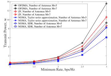
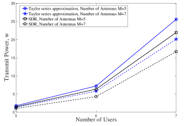
Figure 1: The required total transmit power to achieve different target rates for $3$ users in NOMA, ZF and OFDMA schemes.

Figure 2: The required total transmit power to achieve $R_{k}^{min}=2$ bps/Hz for different numbers of users by using Taylor series approximation and SDR methods.

VI Simulation Results

In this section, the performance of the proposed beamforming designs for the NOMA scheme is evaluated through numerical simulations. We consider a single cell downlink transmission, where a multi-antenna BS serves single-antenna users which are uniformly distributed within the circle with a radius of $50$ meters around the BS, but no closer than $1$ meter. The small-scale fading of the channels is assumed to be Rayleigh fading which represents an isotropic scattering environment. The large-scale fading effect is modelled by ${d_{k}}^{-\beta}$ to incorporate the path-loss effects where $d_{k}$ is the distance between $U_{k}$ and the BS, measured in meters and $\beta$ is the path-loss exponent. Hence, the channel coefficients between the BS and user $U_{k}$ are generated using $\mathbf{h}_{k}=\chi_{k}\sqrt{{d_{k}}^{-\beta}}$ where $\chi_{k}\sim\mathcal{CN}(0,\mathbf{I})$ and $\beta=3.8$ [34]. It should be noted here that in simulations the user distances are fixed and the average is taken over the fast fading component of the channel vectors. It is assumed that the noise variance at each user is 0.01 ($\sigma^{2}=0.01$) and the target rates for all users are the same. The term non-robust scheme refers to the scheme where the BS has imperfect CSI without any information on the channel uncertainties and the beamforming vectors are designed based on imperfect CSI without incorporating channel uncertainty information. In addition, for the imperfect-CSI case the variance of each entry (i.e., $[\mathbf{\Delta}_{k}]_{ij}$ ) of the error covariance matrix $\mathbf{\Delta}_{k}$ and the predefined outage probability ($\rho_{k}$) of the required QoS constraints are set to $0.005$ and $0.1$, respectively. These numerical results are obtained by averaging over different 1000 random channels.

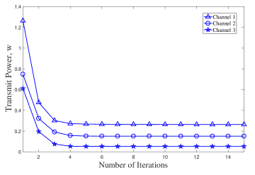
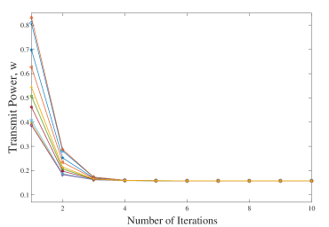
Figure 3: The convergence of the algorithm in Table I for different set of channels. Number of users$=3$,  Number of antennas$=6$,  Target rate$=1$.

Figure 4: The convergence of the algorithm based on Taylor series approximation for different initializations. Number of users$=3$,  Number of antennas$=5$,  Target rate$=1$.

VI-A Power minimization and max-min fairness designs

First, we evaluate the required total transmit power for both power minimization approaches (i.e., Taylor series approximation and SDR) with different system parameters. As can be seen from the figures, the results of these two methods are almost identical. The required total transmit power against different target rates is presented in Fig. 2 for the NOMA and OMA schemes with different numbers of transmit antennas. By increasing the minimum required rate at each user, the BS requires more power to satisfy the target rate requirements. For a given target rate, the required total transmit power can be reduced by employing more antennas at the transmitter. As shown in Fig. 2, for a specific rate requirement, the conventional OMA technique consumes more transmit power than the NOMA scheme. This demonstrates that the NOMA scheme outperforms the conventional OMA in terms of energy efficiency.

In Fig. 2, the required total transmit power for different numbers of users with different numbers of transmit antennas is obtained. As the number of antennas increases, the required transmit power decreases due to the spatial diversity gain. However, the BS requires more transmit power as the number of users increases. As shown in Fig. 2, both schemes, Taylor series approximation and SDR show a similar performance for a few users due to the small number of approximated terms in the Taylor series approximation. However, the number of approximated terms increases with the number of users. As a result, the performance gap between these two schemes increases and SDR outperforms the Taylor series approximation scheme in terms of required transmit power. The reason is that SDR can provide the optimal solution given that the solution is rank one whereas the other scheme relies on the Taylor series approximation which might lead to a suboptimal solution. Fig. 4 depicts the convergence of the algorithm provided in Table I in terms of transmit power. As shown, this approach converges with a small number of iterations (most of the time with $3$ iterations), which does not have a significant impact on the order of the complexity of the proposed algorithm. Moreover, we have numerically evaluated the impact of the initialization of the algorithm on the convergence of the Taylor series approximation. As shown in Fig. 4, the Taylor series approximation method converges to the same solution with different initializations.

Table III is provided to compare the required transmit power for each user and the total transmit power obtained through the Taylor series approximation and SDR approaches. As evidenced by these results, there is no significant difference between the two proposed approaches.

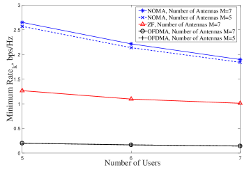
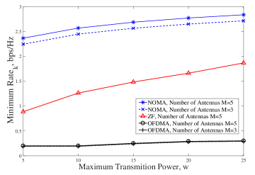
Figure 5: The minimum achieved rate for different numbers of users with $P^{max}=10w$ in NOMA, ZF and OFDMA schemes.

Figure 6: The minimum achieved rate for $5$ users with different $P^{max}$ in NOMA, ZF and OFDMA schemes.

Next, we study the performance of the max-min fairness design for both NOMA and OMA schemes. The balanced rates maintaining fairness between users are demonstrated in Fig. 6 and Fig. 6, respectively, for different numbers of users and maximum available transmit power with different numbers of antennas. As expected, reducing the numbers of users or increasing the maximum available transmit power threshold improves the achievable fairness rate. Since the fairness rate is a logarithmic function of power, as the power threshold increases the rate improvement is compressed. These simulation results confirm that the QoS based beamforming design satisfies the required rate constraints at each user whereas the rates of the users are balanced in the fairness based approach. As shown in Fig. 6 and Fig. 6, for a specific available power, the NOMA scheme achieves more rate than the conventional OMA technique.

The power allocations and the balanced rates obtained by solving problem (33) are provided for five different random channels in Table IV. In order to validate the optimality of the proposed max-min fairness approach, we compare these with the power allocations through the power minimization solution in Section III. In particular, the balanced rates obtained through the fairness approach have been set as the target rates in the power minimization approach for the same set of channels, and the corresponding power allocations are obtained. As seen in Table IV and Table V, both max-min fairness and power minimization approaches utilize the same power allocations to achieve same rates at each user. This confirms the optimality of the proposed max-min fairness based design as the power minimization approach is optimal for a given set of target rates.

VI-B Performance Study of Robust Design

In this subsection, we study the impact of the proposed robust design on the achieved rate in comparison with the non-robust scheme. The effect of error variances on the required transmit power is represented in Fig. 7. It can be observed from Fig. 7 that the total transmit power at the BS increases as the errors in the CSI increase.

We compare the performance of the robust and the non-robust scheme through the rate satisfaction ratio $\eta_{k}$, which is defined as the ratio between the achieved rate and the target rate at the user $U_{k}$. Hence, $\eta_{k}\geq 1$ indicates that the rate requirement is satisfied at the user $U_{k}$.

Fig. 9 and Fig. 9 depict the histogram of the rate satisfaction ratio for the robust and the non-robust schemes with the target rate, $R_{min}=3$, respectively. We also study the rate satisfaction ratio for the robust and the non-robust OMA schemes in Fig. 11 and Fig. 11, respectively. It can be observed that in the robust design, rate constraint is satisfied in most cases and in only $10\%$ of cases does the rate satisfaction ratio fall below one according to the outage probability requirement. However, as evidenced by results presented in Fig. 9 and 11, the non-robust design cannot satisfy the target rate requirement for approximately $50$ percent of the cases since it does not take into account any information regarding channel uncertainties.

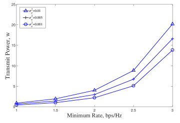
Figure 7: The required total transmit power to achieve different target rates with different channel uncertainties at fix outages $\rho=0.1$. Number of users = Number of antennas = 3.

VII Conclusions

In this paper, we have proposed different beamforming techniques for NOMA based downlink transmission. In particular, these beamforming designs were developed through a) a power minimization approach to achieve the required target rate at each user; b) a max-min fairness approach to maintain user fairness in terms of the achieved rates and c) an outage probability based robust approach to satisfy the target rates with a set of predefined probabilities. To tackle the original non-convex problems, we have developed iterative algorithms by exploiting first order Taylor series approximations and SDR techniques for the first two problems whereas the robust design was solved through converting the non-convex constraints into a set of convex LMIs. Simulation results were provided to validate the performance of the proposed schemes in terms of the required transmit power and balanced rates. These results confirm that the proposed outage probability based robust approach outperforms the non-robust scheme in terms of the achieved rates and rate satisfaction ratio at each user. These simulation results also demonstrate that NOMA can achieve superior performance in terms of system throughput compared to the traditional multiple access and can efficiently utilize the bandwidth resources. In this work, we developed novel resource allocation techniques to improve the system throughput and maintain user fairness, which address the issues associated with multiple access scheme in next generation wireless networks.

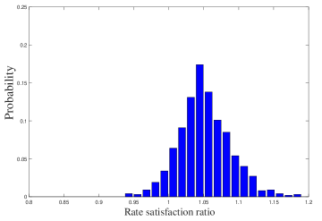
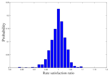
Figure 8: Histogram for rate satisfaction ratio, i.e., $\eta_{k}$, for $R_{min}=3bps/Hz$ in the robust NOMA scheme.

Figure 9: Histogram for rate satisfaction ratio, i.e., $\eta_{k}$, for $R_{min}=3bps/Hz$ in the non-robust NOMA scheme.

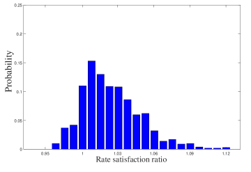
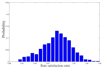
Figure 10: Histogram for rate satisfaction ratio, i.e., $\eta_{k}$, for $R_{min}=3bps/Hz$ in the robust OFDMA scheme.

Figure 11: Histogram for rate satisfaction ratio, i.e., $\eta_{k}$, for $R_{min}=3bps/Hz$ in the non-robust OFDMA scheme.

TABLE III: Comparison of power allocations between Taylor series approximation and SDR approaches

	Taylor Series Approximation Scheme				SDR Scheme
Channels	$\begin{array}[]{c}U_{1}~{}\text{Power}\\ ({\rm w})\end{array}$	$\begin{array}[]{c}U_{2}~{}\text{Power}\\ ({\rm w})\end{array}$	$\begin{array}[]{c}U_{3}~{}\text{Power}\\ ({\rm w})\end{array}$	$\begin{array}[]{c}\text{Total Power}\\ ({\rm w})\end{array}$	$\begin{array}[]{c}U_{1}~{}\text{Power}\\ ({\rm w})\end{array}$	$\begin{array}[]{c}U_{2}~{}\text{Power}\\ ({\rm w})\end{array}$	$\begin{array}[]{c}U_{3}~{}\text{Power}\\ ({\rm w})\end{array}$	$\begin{array}[]{c}\text{Total Power}\\ ({\rm w})\end{array}$
Channel $1$	5.3596	0.6702	0.0821	6.1119	5.3593	0.6701	0.0820	6.1114
Channel $2$	3.7419	0.4692	0.0636	4.2747	3.7417	0.4690	0.0635	4.2742
Channel $3$	7.6185	0.9595	0.1232	8.7012	7.6156	0.9591	0.1230	8.6977
Channel $4$	10.2415	1.2811	0.1642	11.6868	10.2367	1.2808	0.1641	11.6814
Channel $5$	8.4636	1.0626	0.1468	9.6730	8.4634	1.0625	0.1467	9.6726

TABLE IV: Power allocations and achieved rate of the max-min fairness approach

Channels	$\begin{array}[]{c}U_{1}~{}\text{Power}\\ ({\rm w})\end{array}$	$\begin{array}[]{c}U_{2}~{}\text{Power}\\ ({\rm w})\end{array}$	$\begin{array}[]{c}U_{3}~{}\text{Power}\\ ({\rm w})\end{array}$	$\begin{array}[]{c}\text{Total Power}\\ ({\rm w})\end{array}$	$\begin{array}[]{c}U_{1}~{}\text{Rate}\\ (bps/Hz)\end{array}$	$\begin{array}[]{c}U_{2}~{}\text{Rate}\\ (bps/Hz)\end{array}$	$\begin{array}[]{c}U_{3}~{}\text{Rate}\\ (bps/Hz)\end{array}$
Channel $1$	13.9225	0.9990	0.0804	15	3.8010	3.8010	3.8010
Channel $2$	$4.3137$	$0.5965$	$0.0929$	$5$	$2.8584$	$2.8584$	$2.8584$
Channel $3$	9.1271	0.8013	0.0730	10	3.5140	3.5140	3.5140
Channel $4$	6.7110	0.7166	0.0754	7.5	3.2327	3.2327	3.2327
Channel $5$	11.5454	0.8814	0.0752	12.5	3.7119	3.7119	3.7119

TABLE V: Power allocations for a given set target rates (i.e., achieved in fairness approach) through power minimization in (19)

Channels	$\begin{array}[]{c}\text{Target Rate}\\ ({\rm bps/Hz})\end{array}$	$\begin{array}[]{c}\text{Total Power}\\ ({\rm w})\end{array}$	$\begin{array}[]{c}U_{1}~{}\text{Power}\\ ({\rm w})\end{array}$	$\begin{array}[]{c}U_{2}~{}\text{Power}\\ ({\rm w})\end{array}$	$\begin{array}[]{c}U_{3}~{}\text{Power}\\ ({\rm w})\end{array}$
Channel $1$	3.8010	15	13.9225	0.9990	0.0804
Channel $2$	2.8584	5	4.3137	0.5965	0.0929
Channel $3$	3.5140	10	9.1271	0.8013	0.0730
Channel $4$	3.2327	7.5	6.7110	0.7166	0.0754
Channel $5$	3.7119	12.5	11.5454	0.8814	0.0752

Appendix A Proof of Lemma 1

We first summarize the following complex derivatives:

Generalized complex derivative:

$$\frac{\partial f(z)}{\partial z}=\frac{1}{2}\big{(}\frac{\partial f(z)}{\partial\textrm{Re}(z)}-i\frac{\partial f(z)}{\partial\Im(z)}\big{)}$$ (A.1)

Conjugate complex derivative:

$$\frac{\partial f(z)}{\partial z^{*}}=\frac{1}{2}\big{(}\frac{\partial f(z)}{\partial\textrm{Re}(z)}+i\frac{\partial f(z)}{\partial\Im(z)}\big{)}$$ (A.2)

$$\Rightarrow\qquad\frac{\partial f(z)}{\partial\textrm{Re}(z)}=2\textrm{Re}[\frac{\partial f(z)}{\partial z^{*}}],\qquad\frac{\partial f(z)}{\partial\Im(z)}=2\Im[\frac{\partial f(z)}{\partial z^{*}}]$$ (A.3)

Next, we present the first order Taylor series approximation for a function $g(A)$ around $A_{0}$ as follows:

$$g(A)\approx g(A,A_{0})= f(A_{0})+{\rm Tr}\Big{(}\big{[}\frac{\partial f(A_{0})}{\partial\textrm{Re}(A)}\big{]}^{T}\textrm{Re}(A-A_{0})\Big{)}$$

$$+{\rm Tr}\Big{(}\big{[}\frac{\partial f(A_{0})}{\partial\Im(A)}\big{]}^{T}\Im(A-A_{0})\Big{)}$$

$$= f(A_{0})+{\rm Tr}\Big{(}2\big{[}\frac{\partial f(A_{0})}{\partial A^{*}}\big{]}^{T}\textrm{Re}(A-A_{0})\Big{)}$$

$$+{\rm Tr}\Big{(}2\big{[}\frac{\partial f(A_{0})}{\partial A^{*}}\big{]}^{T}\Im(A-A_{0})\Big{)}$$

$$= f(A_{0})+2\textrm{Re}\Big{(}{\rm Tr}\big{[}\frac{\partial f(A_{0})}{\partial A^{*}}\big{]}^{H}(A-A_{0})\Big{)}$$ (A.4)

Based on this first order approximation, we approximate $f_{l}(\mathbf{w}_{k})=\mathbf{w}^{H}_{k}\mathbf{h}_{l}\mathbf{h}_{l}^{H}\mathbf{w}_{k}$ as follows:

$$g_{l}(\mathbf{w}_{k},\mathbf{w}^{t}_{k})= {\mathbf{w}^{t}_{k}}^{H}\mathbf{h}_{l}{\mathbf{h}_{l}}^{H}\mathbf{w}^{t}_{k}$$

$$+\bigg{[}\Big{(}\frac{\partial f_{l}(\mathbf{w}_{k})}{\partial\textrm{Re}(\mathbf{w}_{k})}\Big{|}_{\mathbf{w}_{k}=\mathbf{w}^{t}_{k}}\Big{)}^{T}\textrm{Re}(\mathbf{w}_{k}-\mathbf{w}^{t}_{k})\bigg{]}$$

$$+\bigg{[}\Big{(}\frac{\partial f_{l}(\mathbf{w}_{k})}{\partial\Im(\mathbf{w}_{k})}\Big{|}_{\mathbf{w}_{k}=\mathbf{w}^{t}_{k}}\Big{)}^{T}\Im(\mathbf{w}_{k}-\mathbf{w}^{t}_{k})\bigg{]}$$ (A.5)

The derivatives of the following terms can be written based on the complex derivatives in (A.3):

$$\frac{\partial f_{l}(\mathbf{w}_{k})}{\partial\textrm{Re}(\mathbf{w}_{k})}=2\textrm{Re}(\mathbf{h}_{l}{\mathbf{h}_{l}}^{H}\mathbf{w}_{k}),~{}\frac{\partial f_{l}(\mathbf{w}_{k})}{\partial\Im(\mathbf{w}_{k})}=2\Im(\mathbf{h}_{l}{\mathbf{h}_{l}}^{H}\mathbf{w}_{k}),$$ (A.6)

$$g_{l}(\mathbf{w}_{k},\mathbf{w}^{t}_{k}) = {\mathbf{w}^{t}_{k}}^{H}\mathbf{h}_{l}\mathbf{h}_{l}^{H}\mathbf{w}^{t}_{k}$$ (A.7)

$$+2\big{(}\textrm{Re}({\mathbf{w}^{t}_{k}}^{H}\mathbf{h}_{l}{\mathbf{h}_{l}}^{H})\textrm{Re}(\mathbf{w}_{k}-\mathbf{w}^{t}_{k})\big{)}$$

$$+2\big{(}\Im({\mathbf{w}^{t}_{k}}^{H}\mathbf{h}_{l}{\mathbf{h}_{l}}^{H})\Im(\mathbf{w}_{k}-\mathbf{w}^{t}_{k})\big{)}$$

$$= {\mathbf{w}^{t}_{k}}^{H}\mathbf{h}_{l}\mathbf{h}_{l}^{H}\mathbf{w}^{t}_{k}$$

$$+2\textrm{Re}[{\mathbf{w}^{t}_{k}}^{H}\mathbf{h}_{l}{\mathbf{h}_{l}}^{H}(\mathbf{w}_{k}-\mathbf{w}^{t}_{k})]$$

This completes the proof of Lemma 1.          $\blacksquare$

Appendix B Proof of Lemma 3

In order to convert the probability based constraints in (49) into a tractable form the following lemma is required:

Lemma 3.1: Consider a hermitian random matrix $\mathbf{X}\in\mathbb{C}^{M\times M}$ with each element being independent and identically distributed as $[\mathbf{X}]_{ij}\sim\mathcal{CN}(0,\sigma^{2}_{ij})$. Then, for any hermitian matrix $\mathbf{Y}\in\mathbb{C}^{M\times M}$ , the following holds:

$$\rm{Tr}(\mathbf{YX})\sim\mathcal{CN}(0,\|\mathbf{Y}\odot\Sigma_{X}\|^{2}_{F}),$$

$$\rm{Tr}(\mathbf{YX})=\|\mathbf{Y}\odot\Sigma_{X}\|_{F}U,~{}U\sim\mathcal{N}(0,1),$$

where $\odot$ indicates the Hadamard product and $\Sigma_{X}$ represents a real valued $M\times M$ matrix with each entry $[\Sigma_{X}]_{ij}=\sigma_{ij}$.

By defining a new rank-one positive semidefinite matrix $\mathbf{W}_{k}=\mathbf{w}_{k}\mathbf{w}_{k}^{H}$, the constraints in (49) can be rewritten, respectively, as follows:

$${\rm Pr}\Big{(}{\rm Tr}(-\mathbf{B}_{k}\mathbf{\Delta}_{l})\leq{\rm Tr}(\mathbf{B}_{k}\mathbf{\hat{C}}_{l})-\sigma^{2}\Big{)}\geq(1-\rho_{k}),$$

$$\hskip 42.67912pt\forall k,l=k,k+1,\ldots,N.$$ (B.1)

where $\mathbf{B}_{k}=\gamma_{k}^{-1}\mathbf{W}_{k}-\sum_{m=k+1}^{N}\mathbf{W}_{m}$.

By exploiting Lemma 3.1 and the cumulative distribution function (CDF) of a standard normal distribution, (i.e., ${\rm Pr}(U\leq u)=\frac{1}{2}[1+{\rm erf}(\frac{u}{\sqrt{2}})]$, where $\mathbf{U}\sim\mathcal{N}(0,1)$ ), the inequalities (B.1) can be represented as follows:

$${\rm Pr}\Big{(}{\rm Tr}(-\mathbf{B}_{k}\mathbf{\Delta}_{l})\leq{\rm Tr}(\mathbf{B}_{k}\mathbf{\hat{C}}_{l})-\sigma^{2}\Big{)}$$

$$={\rm Pr}\Big{(}U\leq\frac{{\rm Tr}(\mathbf{B}_{k}\mathbf{\hat{C}}_{l})-\sigma^{2}}{\|-\mathbf{B}_{k}\odot\Sigma_{\mathbf{\Delta}_{l}}\|_{F}}\Big{)}$$

$$=\frac{1}{2}[1+{\rm erf}(\frac{{\rm Tr}(\mathbf{B}_{k}\mathbf{\hat{C}}_{l})-\sigma^{2}}{\sqrt{2}\|-\mathbf{B}_{k}\odot\Sigma_{\mathbf{\Delta}_{l}}\|_{F}})]$$

$$\geq(1-\rho_{k}),$$

$$\forall k,~{}l=k,k+1,\ldots,N,$$ (B.2)

The inequalities in (B.2) can be presented in the following forms,

$$\Phi_{kl}\geq\sqrt{2}~{}{\rm erf}^{-1}(1-2\rho_{k})\|{\rm vec}(-\mathbf{B}_{k}\odot\Sigma_{\mathbf{\Delta}_{l}})\|,$$ (B.3)

where

$$\Phi_{kl}={\rm Tr}(\mathbf{B}_{k}\mathbf{\hat{C}}_{l})-\sigma^{2}.$$ (B.4)

In order to cast the original robust problem into a convex optimization framework, the following lemma is required:

Lemma 3.2: The following second order cone constraint on $x$

$$\|\mathbf{A}x+b\|\leq e^{T}x+d,$$

can be represented with the following linear matrix inequality (LMI):

$$\left[\begin{array}[]{cc}(e^{T}x+d)\mathbf{I}&\mathbf{A}x+b\\ (\mathbf{A}x+b)^{T}&e^{T}x+d\\ \end{array}\right]\succeq 0.$$

By applying Lemma 3.2, the constraints (B.3) can be rewritten as

$$\mathbf{C}_{kl} =\left[\begin{array}[]{cc}\frac{\Phi_{kl}}{\sqrt{2}{\rm erf}^{-1}(1-2\rho_{k})}\mathbf{I}_{M^{2}}&{\rm vec}(-\mathbf{B}_{k}\odot\Sigma_{\mathbf{\Delta}_{l}})\\ {\rm vec}^{H}(-\mathbf{B}_{k}\odot\Sigma_{\mathbf{\Delta}_{l}})&\frac{\Phi_{kl}}{\sqrt{2}{\rm erf}^{-1}(1-2\rho_{k})}\\ \end{array}\right],$$ (B.7)

$$\qquad\qquad\forall k,~{}l=k,k+1,\ldots,N.$$ (B.8)

This completes the proof of Lemma 3.        $\blacksquare$

References

- [1] M. Al-Imari, P. Xiao, M. A. Imran, and R. Tafazolli, “Uplink non-orthogonal multiple access for 5G wireless networks,” in Proc. 11th International Symposium on Wireless Communications Systems (ISWCS), August 2014, pp. 781–785.
- [2] F. Alavi, K. Cumanan, Z. Ding, and A. G. Burr, “Robust beamforming techniques for non-orthogonal multiple access systems with bounded channel uncertainties,” IEEE Communications Letters, vol. 21, no. 9, pp. 2033–2036, September 2017.
- [3] F. Alavi, K. Cumanan, Z. Dingl, and A. G. Burr, “Outage constraint based robust beamforming design for non-orthogonal multiple access in 5G cellular networks,” in Proc. IEEE International Symposium on Personal, Indoor, and Mobile Radio Communications (PIMRC), October 2017, pp. 1–5.
- [4] F. Alavi, N. Mokari, and H. Saeedi, “Secure resource allocation in OFDMA-based cognitive radio networks with two-way relays,” in Proc. Iranian Conference on Electrical Engineering, May 2015, pp. 171–176.
- [5] F. Alavi and H. Saeedi, “Radio resource allocation to provide physical layer security in relay-assisted cognitive radio networks,” IET Communications, vol. 9, no. 17, pp. 2124–2130, 2015.
- [6] F. Alavi, N. M. Yamchi, M. R. Javan, and K. Cumanan, “Limited feedback scheme for device-to-device communications in 5G cellular networks with reliability and cellular secrecy outage constraints,” IEEE Transactions on Vehicular Technology, vol. 66, no. 9, pp. 8072–8085, September 2017.
- [7] M. Bengtsson and B. Ottersten, “Optimal downlink beamforming using semidefinite optimization,” in Proc. Allerton Conference on Communication, Control, and Computing, September 1999, pp. 987–996.
- [8] ——, Optimal and suboptimal transmit beamforming. Handbook of Antennas in Wireless Communications, CRC Press, 2001.
- [9] A. Benjebbour, Y. Saito, Y. Kishiyama, A. Li, A. Harada, and T. Nakamura, “Concept and practical considerations of non-orthogonal multiple access (NOMA) for future radio access,” in Proc. International Symposium on Intelligent Signal Processing and Communications Systems (ISPACS), November 2013, pp. 770–774.
- [10] E. Björnson and E. Jorswieck, Optimal Resource Allocation in Coordinated Multi-Cell Systems. Now Foundations and Trends, 2013, vol. 9, no. 2-3.
- [11] X. Chen, Z. Zhang, C. Zhong, and D. W. K. Ng, “Exploiting multiple-antenna techniques for non-orthogonal multiple access,” IEEE Journal on Selected Areas in Communications, vol. 35, no. 10, pp. 2207–2220, October 2017.
- [12] J. Choi, “Minimum power multicast beamforming with superposition coding for multiresolution broadcast and application to NOMA systems,” IEEE Transactions on Communications, vol. 63, no. 3, pp. 791–800, March 2015.
- [13] K. Cumanan, G. C. Alexandropoulos, Z. Ding, and G. K. Karagiannidis, “Secure communications with cooperative jamming: Optimal power allocation and secrecy outage analysis,” IEEE Transactions on Vehicular Technology, vol. 66, no. 8, pp. 7495–7505, August 2017.
- [14] K. Cumanan, Z. Ding, Y. Rahulamathavan, M. M. Molu, and H. H. Chen, “Robust MMSE beamforming for multiantenna relay networks,” IEEE Transactions on Vehicular Technology, vol. 66, no. 5, pp. 3900–3912, May 2017.
- [15] K. Cumanan, Z. Ding, B. Sharif, G. Y. Tian, and K. K. Leung, “Secrecy rate optimizations for a MIMO secrecy channel with a multiple-antenna eavesdropper,” IEEE Transactions on Vehicular Technology, vol. 63, no. 4, pp. 1678–1690, May 2014.
- [16] K. Cumanan, R. Krishna, V. Sharma, and S. Lambotharan, “Robust interference control techniques for cognitive radios using worst-case performance optimization,” in Proc. International Symposium on Information Theory and Its Applications, December 2008, pp. 1–5.
- [17] K. Cumanan, R. Krishna, Z. Xiong, and S. Lambotharan, “Multiuser spatial multiplexing techniques with constraints on interference temperature for cognitive radio networks,” IET Signal Processing, vol. 4, no. 6, pp. 666–672, December 2010.
- [18] K. Cumanan, L. Musavian, S. Lambotharan, and A. B. Gershman, “SINR balancing technique for downlink beamforming in cognitive radio networks,” IEEE Signal Processing Letters, vol. 17, no. 2, pp. 133–136, February 2010.
- [19] K. Cumanan, H. Xing, P. Xu, G. Zheng, X. Dai, A. Nallanathan, Z. Ding, and G. K. Karagiannidis, “Physical layer security jamming: Theoretical limits and practical designs in wireless networks,” IEEE Access, vol. 5, pp. 3603–3611, 2017.
- [20] K. Cumanan, R. Zhang, and S. Lambotharan, “A new design paradigm for MIMO cognitive radio with primary user rate constraint,” IEEE Communications Letters, vol. 16, no. 5, pp. 706–709, May 2012.
- [21] L. Dai, B. Wang, Y. Yuan, S. Han, C. L. I, and Z. Wang, “Non-orthogonal multiple access for 5G: solutions, challenges, opportunities, and future research trends,” IEEE Communications Magazine, vol. 53, no. 9, pp. 74–81, September 2015.
- [22] Z. Ding, P. Fan, and H. V. Poor, “Impact of user pairing on 5G nonorthogonal multiple-access downlink transmissions,” IEEE Transactions on Vehicular Technology, vol. 65, no. 8, pp. 6010–6023, August 2016.
- [23] Z. Ding, M. Peng, and H. V. Poor, “Cooperative non-orthogonal multiple access in 5G systems,” IEEE Communications Letters, vol. 19, no. 8, pp. 1462–1465, August 2015.
- [24] Z. Ding and H. V. Poor, “Design of massive-MIMO-NOMA with limited feedback,” IEEE Signal Processing Letters, vol. 23, no. 5, pp. 629–633, May 2016.
- [25] Z. Ding, R. Schober, and H. V. Poor, “A general MIMO framework for NOMA downlink and uplink transmission based on signal alignment,” IEEE Transactions on Wireless Communications, vol. 15, no. 6, pp. 4438–4454, June 2016.
- [26] Z. Ding, F. Adachi, and H. V. Poor, “The application of MIMO to non-orthogonal multiple access,” IEEE Transactions on Wireless Communications, vol. 15, no. 1, pp. 537–552, January 2016.
- [27] Z. Ding, Z. Yang, P. Fan, and H. V. Poor, “On the performance of non-orthogonal multiple access in 5G systems with randomly deployed users,” IEEE Signal Processing Letters, vol. 21, no. 12, pp. 1501–1505, December 2014.
- [28] M. Fozooni, A. Abbasfar, and A. Sani, “Spectrum sharing in heavy loaded networks,” in Proc. International Telecommunications Network Strategy and Planning Symposium (NETWORKS), October 2012, pp. 1–5.
- [29] M. Fozooni, M. Matthaiou, E. Bjornson, and T. Q. Duong, “Performance limits of MIMO systems with nonlinear power amplifiers,” in Proc. IEEE Global Communications Conference (GLOBECOM), December 2015, pp. 1–7.
- [30] M. Fozooni, M. Matthaiou, S. Jin, and G. C. Alexandropoulos, “Massive MIMO relaying with hybrid processing,” in Proc. IEEE International Conference on Communications (ICC), May 2016, pp. 1–6.
- [31] M. F. Hanif, Z. Ding, T. Ratnarajah, and G. K. Karagiannidis, “A minorization-maximization method for optimizing sum rate in the downlink of non-orthogonal multiple access systems,” IEEE Transactions on Signal Processing, vol. 64, no. 1, pp. 76–88, January 2016.
- [32] K. Higuchi and Y. Kishiyama, “Non-orthogonal access with random beamforming and intra-beam SIC for cellular MIMO downlink,” in IEEE 78th Vehicular Technology Conference (VTC Fall), September 2013, pp. 1–5.
- [33] S. M. R. Islam, N. Avazov, O. A. Dobre, and K. S. Kwak, “Power-domain non-orthogonal multiple access (NOMA) in 5G systems: Potentials and challenges,” IEEE Communications Surveys Tutorials, vol. 19, no. 2, pp. 721–742, 2017.
- [34] M. R. Javan, N. Mokari, F. Alavi, and A. Rahmati, “Resource allocation in decode-and-forward cooperative communication networks with limited rate feedback channel,” IEEE Transactions on Vehicular Technology, vol. 66, no. 1, pp. 256–267, January 2017.
- [35] S. K. Joshi, U. L. Wijewardhana, M. Codreanu, and M. Latva-aho, “Maximization of worst-case weighted sum-rate for MISO downlink systems with imperfect channel knowledge,” IEEE Transactions on Communications, vol. 63, no. 10, pp. 3671–3685, October 2015.
- [36] B. Kimy, S. Lim, H. Kim, S. Suh, J. Kwun, S. Choi, C. Lee, S. Lee, and D. Hong, “Non-orthogonal multiple access in a downlink multiuser beamforming system,” in Proc. IEEE Military Communications Conference (MILCOM), November 2013, pp. 1278–1283.
- [37] Q. Li, H. Niu, A. Papathanassiou, and G. Wu, “5G network capacity: key elements and technologies,” IEEE Vehicular Technology Magazine, vol. 9, no. 1, pp. 71–78, March 2014.
- [38] Y. Li, M. Jiang, Q. Zhang, Q. Li, and J. Qin, “Secure beamforming in downlink MISO nonorthogonal multiple access systems,” IEEE Transactions on Vehicular Technology, vol. 66, no. 8, pp. 7563–7567, August 2017.
- [39] Z. Liu, L. Lei, N. Zhang, G. Kang, and S. Chatzinotas, “Joint beamforming and power optimization with iterative user clustering for MISO-NOMA systems,” IEEE Access, 2017.
- [40] S. B. M. S. Lobo, L. Vandenberghe and H. Lebret, “Applications of second-order cone programming,” Linear Algebra Appl., Special Issue on Linear Algebra in Control, Signals and Image Processing, pp. 193–228, November 1998.
- [41] N. Mokari, F. Alavi, S. Parsaeefard, and T. Le-Ngoc, “Limited-feedback resource allocation in heterogeneous cellular networks,” IEEE Transactions on Vehicular Technology, vol. 65, no. 4, pp. 2509–2521, April 2016.
- [42] S. Nasseri and M. R. Nakhai, “Robust interference management via outage-constrained downlink beamforming in multicell networks,” in Proc. IEEE Global Communications Conference (GLOBECOM), December 2013, pp. 3470–3475.
- [43] I. Polik and T. Terlaky, Interior Point Methods for Nonlinear Optimization. New York, NY, USA: Springer, 2010.
- [44] Y. Saito, Y. Kishiyama, A. Benjebbour, T. Nakamura, A. Li, and K. Higuchi, “Non-orthogonal multiple access (NOMA) for cellular future radio access,” in Proc. IEEE Vehicular Technology Conference (VTC Spring), June 2013, pp. 1–5.
- [45] M. Schubert and H. Boche, “Solution of the multiuser downlink beamforming problem with individual SINR constraints,” IEEE Transactions on Vehicular Technology, vol. 53, no. 1, pp. 18–28, January 2004.
- [46] C. Shen, T. H. Chang, K. Y. Wang, Z. Qiu, and C. Y. Chi, “Chance-constrained robust beamforming for multi-cell coordinated downlink,” in Proc. IEEE Global Communications Conference (GLOBECOM), December 2012, pp. 4957–4962.
- [47] C. Shen, T.-H. Chang, K.-Y. Wang, Z. Qiu, and C.-Y. Chi, “Distributed robust multicell coordinated beamforming with imperfect CSI: An ADMM approach,” IEEE Transactions on Signal Processing, vol. 60, no. 6, pp. 2988–3003, June 2012.
- [48] Q. Sun, S. Han, C. L. I, and Z. Pan, “On the ergodic capacity of MIMO NOMA systems,” IEEE Wireless Communications Letters, vol. 4, no. 4, pp. 405–408, August 2015.
- [49] M. Tian, Q. Zhang, S. Zhao, Q. Li, and J. Qin, “Secrecy sum rate optimization for downlink MIMO nonorthogonal multiple access systems,” IEEE Signal Processing Letters, vol. 24, no. 8, pp. 1113–1117, August 2017.
- [50] S. Timotheou and I. Krikidis, “Fairness for non-orthogonal multiple access in 5G systems,” IEEE Signal Processing Letters, vol. 22, no. 10, pp. 1647–1651, October 2015.
- [51] WhitePaper, “Rethink mobile communications for 2020+,” Future Mobile Communication Forum 5G SIG, November 2014.
- [52] G. Wunder, P. Jung, M. Kasparick, T. Wild, F. Schaich, Y. Chen, S. T. Brink, I. Gaspar, N. Michailow, A. Festag, L. Mendes, N. Cassiau, D. Ktenas, M. Dryjanski, S. Pietrzyk, B. Eged, P. Vago, and F. Wiedmann, “5GNOW: non-orthogonal, asynchronous waveforms for future mobile applications,” IEEE Communications Magazine, vol. 52, no. 2, pp. 97–105, February 2014.
- [53] P. Xu and K. Cumanan, “Optimal power allocation scheme for non-orthogonal multiple access with -fairness,” IEEE Journal on Selected Areas in Communications, vol. 35, no. 10, pp. 2357–2369, October 2017.
- [54] P. Xu, K. Cumanan, and Z. Yang, “Optimal power allocation scheme for NOMA with adaptive rates and alpha-fairness,” in Proc. IEEE Global Communications Conference (GLOBECOM), December 2017, pp. 1–6.
- [55] P. Xu, Z. Ding, X. Dai, and H. V. Poor, “A new evaluation criterion for non-orthogonal multiple access in 5G software defined networks,” IEEE Access, vol. 3, pp. 1633–1639, 2015.
- [56] C. Xue, Q. Zhang, Q. Li, and J. Qin, “Joint power allocation and relay beamforming in nonorthogonal multiple access amplify-and-forward relay networks,” IEEE Transactions on Vehicular Technology, vol. 66, no. 8, pp. 7558–7562, August 2017.
- [57] L. Zhang, R. Zhang, Y. C. Liang, Y. Xin, and H. V. Poor, “On gaussian MIMO BC-MAC duality with multiple transmit covariance constraints,” IEEE Transactions on Information Theory, vol. 58, no. 4, pp. 2064–2078, April 2012.
- [58] Q. Zhang, Q. Li, and J. Qin, “Robust beamforming for non-orthogonal multiple-access systems in MISO channels,” IEEE Transactions on Vehicular Technology, vol. 65, no. 12, pp. 10 231–10 236, December 2016.
- [59] R. Zhang and L. Hanzo, “A unified treatment of superposition coding aided communications: Theory and practice,” IEEE Communications Surveys Tutorials, vol. 13, no. 3, pp. 503–520, 2011.