On the Ergodic Control of Ensembles

Abstract

Across smart-grid and smart-city application domains, there are many problems where an ensemble of agents is to be controlled such that both the aggregate behaviour and individual-level perception of the system’s performance are acceptable. In many applications, traditional PI control is used to regulate aggregate ensemble performance. Our principal contribution in this note is to demonstrate that PI control may not be always suitable for this purpose, and in some situations may lead to a loss of ergodicity for closed-loop systems. Building on this observation, a theoretical framework is proposed to both analyse and design control systems for the regulation of large scale ensembles of agents with a probabilistic intent. Examples are given to illustrate our results.

1 Introduction

At a very high level, smart-city related research concerns designing systems that endeavour to make the best use of limited resources across a number of domains (energy, transport, water etc). While classical control has much to offer in such application areas, there are aspects and peculiarities of many of these applications that require practitioners in Control Theory to explore new types of theoretical and practical challenges. Roughly speaking, classical control is typically concerned with regulating a single system, such that the system achieves a desired behaviour in an optimal way. In contrast, in many smart city applications, we are interested in allocating a resource among a population of agents. These might be humans or algorithmic processes that bid for access to a resource in some probabilistic manner (for example, access to part of a road network). In such applications, both the experience of the individual, and their aggregate effect are important. Furthermore, in smart-city applications, we typically wish to control and influence the behaviour of large-scale populations, where the number of agents varies over time and is not known with certainty. Additionally, there are limits to the observability of such systems and data sets are often obtained in a closed-loop fashion; that is, operator’s decisions are often reflected in the data sets. Finally, a fundamental difference between classical control and smart-grid and smart-city control is the need to study the effect of a common control signal on the individual agent and its long term access to a constrained resource. Among all of these fundamental differences, it is this last issue that is perhaps most alien to the classical control theorist, and yet the issue that is perhaps the most pressing in real-life applications, since the need for predictability, at the level of individual agents, underpins an operator’s ability to write economic contracts.

In this paper, our starting point is the observation that many problems that are considered in smart-grids and smart-cities can be cast in a framework where a large number of agents, such as people, cars, or machines, often with unknown objectives, compete for a limited resource. The challenge of allocating this resource in a manner that is not wasteful, which gives an optimal return on the use of the resource for society, and which, in addition, gives a guaranteed level of service to each of the agents competing for that resource, gives rise to a whole host of problems, which in principle are best addressed in a control-theoretic manner. From the perspective of a control engineer, this statement can be decomposed into three objectives; two of which are familiar in control, and the other one constitutes a relatively new consideration. Our first objective is to fully utilise the resource, which is a regulation problem. Second, we would then like to make optimal use of the resource. While both of these objectives are concerned with the aggregate behaviour of an agent population, they make no attempt to control the manner in which the agents orchestrate their behaviour to achieve this aggregate effect. Our third objective thus focuses on the effects of the control on the microscopic properties of the agent population. Ultimately, this third objective can be phrased in terms of properties of the stochastic process capturing the share of the resource that is allocated to an individual agent. For example, we may wish that each agent, on average, receives a fair share of the resource over time, or, at a much more fundamental level, we wish the average allocation of the resource to each agent over time to be a stable quantity that is entirely predictable and which does not depend on initial conditions, and which is not sensitive to noise entering the system. From the point of view of the design of the feedback system, these latter concerns are related to the existence of the unique invariant measure that governs the distribution of the resource amongst the agents in the long run. Thus, the design of feedback systems for deployment in multi-agent applications must consider not only the traditional notions of regulation and optimisation, but also the guarantees concerning the existence of this unique invariant measure. As we shall see, this is not a trivial task and many familiar control strategies, in very simple situations, do not necessarily give rise to feedback systems which possess all three of these features.

1.1 Brief overview of related work

Due to the intrinsically multidisciplinary nature of the problem studied in this paper, related topics are discussed in several communities. As stated before, several problems in smart cities and smart grid can be seen as the task of efficiently allocating some resource among a population of agents, even though there is no formal and widely accepted definition for “smart city” (Zanella et al., 2014). Intelligent transportation systems (ITS), for instance, are one of the many smart-city application areas that thrived in the last few years, presenting rapid technological developments due to (i) the integration of transportation systems with the Internet and (ii) the pressure for green – environmentally friendly – transport solutions. Typical applications in ITS vary from monitoring and controlling transportation flows (Chen and Cheng, 2010) and $CO_{2}$ emissions (Schlote et al., 2013) to assigning parking spaces (Schlote et al., 2014) and utilising vehicle-to-grid (V2G) energy supply (Shaukat et al., 2018, Pillai and Bak-Jensen, 2011). In the context of smart grids, problems related to real-time electricity pricing (Mohsenian-Rad and Leon-Garcia, 2010), real-time demand response (Conejo et al., 2010, Callaway and Hiskens, 2011), and real-time interruptible loads management (Caves et al., 1988, Alagoz et al., 2013, Salsbury et al., 2013) and V2G-related issues, have also attracted interest over the last few years. For these – and many other – applications, we present both conditions ensuring and ruling out ergodicity in a certain closed-loop sense. Related work also appears in the context of multi-agent systems (McArthur et al., 2007). Multi-agent systems arise, for instance, in the application areas stated above, and many references in the literature address these problems using ideas based on consensus or agreement (Blondel et al., 2005, Nedić and Ozdaglar, 2009). The consensus approach is very useful in practice, due to its strong links to utility maximization and fairness. The concept of fairness can be related to ergodicity, as an ergodic dynamic behaviour implies several important properties that are necessary for fairness (Mathew and Mezić, 2011). Finally, we note that our positive results in this paper are based on iterated function systems (Elton, 1987, Barnsley et al., 1988, 1989). Iterated function systems (IFS), albeit not well known in the control community, are a convenient and rich class of Markov processes. As it will be seen in the sequel, a class of stochastic systems arising from the dynamics of multi-agent interactions can be modelled and analysed using IFS in a particularly natural way. The use of IFS makes it possible to obtain strong stability guarantees for such stochastic systems. To prove certain contrapositive statements, suggesting when such guarantees are impossible to provide, we use novel coupling arguments of Hairer et al. (Hairer et al., 2011). Our use of coupling arguments to prove such negative results is one of the first within Control Theory, as far as we know.

1.2 Paper Organisation and Contributions

The main purpose of the present paper is to introduce and analyse the main features of a problem class which is of great interest for smart cities applications. Our main contributions, apart from formulating the problem class itself, arise from the study of the ergodic properties associated with output-regulation problems in such multi-agent settings. At a high level, we show the following:

• In regulating the behaviour of ensembles of agents, feedback control with integral action may destroy the ergodic properties of the closed-loop system, even when the agent behaviour is benign and despite the fact that regulation is achieved. The importance of this result stems from the fact that ergodic behaviour is a fundamental property that is essential for underpinning economic contracts, and for guaranteeing properties such as fairness. The result is hence important from a practical context, and is not merely of theoretical interest.

• We present specific examples to illustrate the loss of ergodicity in very benign examples.

• We show that for certain population types and filters, stable control action always results in ergodic behaviour. In particular, we show this for linear and non-linear systems, with both real-valued actions, and for actions constrained to a finite set.

• A final minor contribution is to illustrate the use of results from the study of iterated function systems in designing controllers for certain classes of dynamic systems.

Given the widespread interest in applications where the behaviour of ensembles of rational agents are orchestrated with probabilistic intent, we believe that these results may be of interest in these and related areas.

The paper is organised as follows: In Section 2, we present our model. We then formulate the necessary concepts from the theory of Markov chains we will use, and recall the concept of coupling of invariant measures in order to state a necessary condition for ergodicity. In Section 3.1, we present a negative result, which shows that ergodicity may fail whenever a standard PI controller is used in the loop. In particular, the amount of a resource that can be used by a particular agent depends on the initial state of the controller. In Section 3.2, a positive result is obtained for stable linear controllers. In Sections 4.1, and 4.2, we extend the results to non-linear systems and cases where actions are constrained to a finite set, respectively.

Remark 1.

A preliminary version of this paper has appeared in (Fioravanti et al., 2017). The present paper extends beyond this preliminary version in several ways. First, full proofs are given. Second, additional positive results are developed for both linear and non-linear systems with both continuous and finite sets of actions. Finally, examples illustrating loss of ergodicity are presented.

2 Preliminaries

We now develop the general setting of this paper. The objective here is to set out our modelling framework, and to present basic results that can be useful in studying the properties of control strategies for ensembles.

2.1 Notation

In general, our notation employs the following rules: Upper-case letters are used for matrices, in caligraphic they denote groups, maps, operators, and in blackboard-bold the probability operator $\mathbb{P}$ as well as sets, and spaces while lower-case letters are used for vectors, scalars, and functions. Subscripts are used to distinguish symbols; time-indexed symbols are followed by the time index in parentheses, as in $x(k)$. Superscript is used for exponentiation and, in $(\cdot)^{T}$, for the transpose operation. For a given measurable space $(\mathbb{X},{\mathscr{F}})$, with $\sigma$-algebra ${\mathscr{F}}$, $M(\mathbb{X})$ indicates the set of all probability measures over $\mathbb{X}$ and $\mathbb{X}^{\infty}$ denotes its associated path space, which consists of infinite right-sided sequences over $\mathbb{X}$: $x(0)\in\mathbb{X},x(1)\in\mathbb{X},x(2)\in\mathbb{X},\ldots$. Details of the notation are introduced locally in the sections, where it is first utilised. For a complete listing of the symbols utilised, please see the supplementary material on-line.

2.2 Models

We consider the problem of repeatedly distributing a limited resource among multiple agents, based on some information concerning the resource, which is provided by a central authority. Throughout, we consider systems subject to several constraints. First, the central authority does not observe the consumption of individual agents, but rather the total utilisation of the resource, or a filtered version thereof. Based on the filtered measurements of the utilisation, the central authority provides information to the agents, sets the price of utilising the resource, or similar. Second, the agents respond to information broadcast by the central authority, but have only limited communication capability otherwise. Specifically, we assume no inter-agent communication. Third, the agents have their own, private objectives. That is, although they receive information from the central authority, they need not pick an action the authority would deem most appropriate. As we shall see, it will be convenient to encode the selfish response of an agent to the information in a probabilistic manner. Finally, in our model, the agents may be limited to a choice from a finite set of possible requests for the resource. In an extreme case, the agents only have the possibility to turn their utilisation on or off, i.e. $x_{i}\in\{0,1\}$. In a more general setting, a subpopulation might be able to choose their consumption from a continuous interval or via some local control.

With these constraints in mind, we are interested in the closed-loop, discrete time system depicted in Figure 1, comprising a controller, a number $N\in\mathbb{N}$ of agents, and a filter. A controller $\mathscr{C}$, which represents the central authority, produces a signal $\pi(k)$ at time $k$. In response, the agents, modelled by systems $\mathscr{S}_{1}$, $\mathscr{S}_{2}$, …, $\mathscr{S}_{N}$, amend their use of the resource. The internal state of the agents is denoted by $x_{i}$, $i=1,\ldots,N$. In particular, $x_{i}(k)$ is a random variable. We model the use of the resource $y_{i}(k)$ of agent $i$ at time $k$ as the output of system ${\mathscr{S}}_{i}$, which is again a random variable. In the remainder we will assume $y_{i}(k)$ and $\pi(k)$ are scalars, but generalisations are easy to obtain. The randomness can be a result of the inherent randomness in the reaction of user $i$ to the control signal $\pi(k)$, or the response to a control signal that is intentionally randomized (Schlote et al., 2013, 2014, Marecek et al., 2015). The aggregate resource utilisation $y(k)\mathrel{\mathop{:}}=\sum_{i=1}^{N}y_{i}(k)$ at time $k$ is then also a random variable. The controller may not have access to either $x_{i}(k)$, $y_{i}(k)$ or $y(k)$, but only to the error signal $e(k)$, which is the difference of $\hat{y}(k)$, the output of a filter $\mathscr{F}$, and $r$, the desired value of $y(k)$. Further, we assume that the controller has its private state $x_{c}(k)\in\mathbb{R}^{n_{c}}$. The controller aims to regulate the system by providing a signal $\pi(k)\in\Pi\subseteq\mathbb{R}$ at time $k$; here, $\Pi$ denotes the set of admissible broadcast control signals. In the simpler static case, the signal $\pi(k)$ is a function of an error signal $e(k)$ and the controller state $x_{c}(k)$, whose range is $\Pi$.

In the case of purely discrete agents, the non-deterministic agent-specific response to the feedback signal $\pi(k)\in\Pi$ can be modelled by agent-specific and signal-specific probability distributions over certain agent-specific set of actions $\mathbb{A}_{i}=\{a_{1},\ldots,a_{L}\}\subset\mathbb{R}^{n_{i}}$, where $\mathbb{R}^{n_{i}}$ can be seen as the space of agent’s $i$ private state $x_{i}$. Assume that the set of possible resource demands of agent $i$ is $\mathbb{D}_{i}$, where in the case that $\mathbb{D}_{i}$ is finite we denote

$$\mathbb{D}_{i}:=\{d_{i,1},d_{i,2},\ldots,d_{i,m_{i}}\}.$$ (1)

In the general case, we assume there are $w_{i}\in\mathbb{N}$ state transition maps ${\mathscr{W}}_{ij}:\mathbb{R}^{n_{i}}\to\mathbb{R}^{n_{i}}$, $j=1,\ldots,w_{i}$ for agent $i$ and $h_{i}\in\mathbb{N}$ output maps ${\mathscr{H}}_{i\ell}:\mathbb{R}^{n_{i}}\to\mathbb{D}_{i}$, $\ell=1,\ldots,h_{i}$ for each agent $i$. The evolution of the states and the corresponding demands then satisfy:

$$x_{i}(k+1) \in\{{\mathscr{W}}_{ij}(x_{i}(k))\;|\;j=1,\ldots,w_{i}\},$$ (2)

$$y_{i}(k) \in\{{\mathscr{H}}_{i\ell}(x_{i}(k))\;|\;\ell=1,\ldots,h_{i}\},$$ (3)

where the choice of agent $i$’s response at time $k$ is governed by probability functions $p_{ij}:\Pi\to[0,1]$, $j=1,\ldots,w_{i}$, respectively $p^{\prime}_{i\ell}:\Pi\to[0,1]$, $\ell=1,\ldots,h_{i}$. Specifically, for each agent $i$, we have for all $k\in\mathbb{N}$ that

$$\mathbb{P}\big{(}x_{i}(k+1)={\mathscr{W}}_{ij}(x_{i}(k))\big{)}=p_{ij}(\pi(k)),$$ (4a)

$$\mathbb{P}\big{(}y_{i}(k)={\mathscr{H}}_{i\ell}(x_{i}(k))\big{)}=p^{\prime}_{i\ell}(\pi(k)).$$ (4b)

Additionally, for all $$\pi\in\Pi i=1,\ldots,N$$, it holds that

$$\sum_{j=1}^{w_{i}}p_{ij}(\pi)=\sum_{\ell=1}^{h_{i}}p^{\prime}_{i\ell}(\pi)=1.$$ (4c)

The final equality comes from the fact $p_{ij}$, $p^{\prime}_{i\ell}$ are probability functions. We assume that, conditioned on $\{x_{i}(k)\},\pi(k)$, the random variables $\{x_{i}(k+1)\mid i=1,\ldots,N\}$ are stochastically independent. The outputs $y_{i}(k)$ each depend on $x_{i}(k)$ and the signal $\pi(k)$ only. As we shall see, this general framework allows for surprisingly sharp results.

Our specific aim is to distribute the resource such that we achieve the following goals almost surely, i.e. with probability $1$:

1. feasibility: Given an upper bound $r>0$ for the utilization of the resource, we require for all $k\in\mathbb{N}$

   $$\sum_{i=1}^{N}y_{i}(k)=y(k)\leq r.$$ (5)

   More generally, the resource could be time-varying; for the purposes of this paper it will assumed to be a constant quantity.

2. predictability: for each agent $i$ there exists a constant $\overline{r}_{i}$ such that

   $$\lim_{k\to\infty}\frac{1}{k+1}\sum_{j=0}^{k}y_{i}(j)=\overline{r}_{i},$$ (6)

   where this latter limit is independent of initial conditions.

Further optional requirements may include: fairness, which could be formulated by saying that all the $\overline{r}_{i}$ coincide, and optimality so that the vector $\overline{r}=\begin{bmatrix}\overline{r}_{1}&\ldots&\overline{r}_{N}\end{bmatrix}$ is a local optimum of an underlying optimization problem. In addition, it is also of interest to achieve the goals after a transient phase, i.e. for all $k\geq K$, where $K$ is a constant.

While all of these goals are important from a practical perspective, the principal property of interest in this paper is the goal of predictability, since this latter issue defines the ability of service providers to write economic contracts. In order to analyze this more formally, we consider an augmented state space $\mathbb{X}\subset\mathbb{R}^{d}$, which captures the state of the controller, the filter, and the agents. Denote by $M(\mathbb{X})$ the space of probability measures over $\mathbb{X}$ with the standard $\sigma$-algebra. The behaviour of the overall system in response to the signal $\pi(k)$ can be modelled as $P:\mathbb{X}\times\Pi\to M(\mathbb{X})$. In order to reason about the evolution of the state, consider the space $\mathbb{X}^{\infty}$ of one-sided infinite sequences of states, known as the path space. Further, we introduce the space of probability measures on path space $\mathbb{X}^{\infty}$ with the product $\sigma$-algebra. Notice that for a particular combination of a filter ${\mathscr{F}}$, controller ${\mathscr{C}}$, and population of agents, the feedback loop can be modelled by an operator $\mathscr{P}_{k}:M(\mathbb{X})\to M(\mathbb{X})$ and the associated dynamical system $(\mathscr{P}_{k})_{k\in\mathbb{N}}$. Our paper, at some level, asks what properties of ${\mathscr{C}}$ and ${\mathscr{F}}$ make $(\mathscr{P}_{k})_{k\in\mathbb{N}}$ predictable and what properties of ${\mathscr{C}}$ render it impossible for it to be predictable. Predictability is related to asymptotic convergence in probability in terms of measures over the path space, i.e., $M(\mathbb{X}^{\infty})$, and will be conveniently characterised in the next section in terms of the existence of a unique invariant measure, in the language of Markov chains.

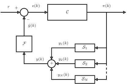
Figure 1: Feedback model.

2.3 Markov Chains and Iterated Function Systems

The set-up described in the prequel resembles closely that of an iterated function system (Elton, 1987, Barnsley et al., 1988, 1989). Iterated function systems are a class of stochastic dynamic systems, for which strong stability and convergence results exist. We now introduce some notation and mention some of the most important results.

To begin, let $\Sigma$ be a closed subset of $\mathbb{R}^{n}$ with the usual Borel $\sigma$-algebra $\mathbb{B}(\Sigma)$. We call the elements of $\mathbb{B}$ events. A Markov chain on $\Sigma$ is a sequence of $\Sigma$-valued random vectors $\{X(k)\}_{k\in\mathbb{N}}$ with the Markov property, which is the equality of a probability of an event conditioned on past events and probability of the same event conditioned on the current state, i.e., we always have

$$\mathbb{P}\left(X(k+1)\in\mathbb{G}\mid X(j)=x_{j},\,j=0,1,\dots,k\right)$$

$$=\mathbb{P}\big{(}X(k+1)\in\mathbb{G}\mid X(k)=x_{k}\big{)},$$

where $\mathbb{G}$ is an event and $k\in\mathbb{N}$. We assume the Markov chain is time-homogeneous. The transition operator $P$ of the Markov chain is defined for $x\in\Sigma$, $\mathbb{G}\in\mathbb{B}$ by

$$P(x,\mathbb{G}):=\mathbb{P}(X(k+1)\in\mathbb{G}\;|\;X(k)=x).$$

If the initial condition $X_{0}$ is distributed according to an initial distribution $\lambda$, we denote by $\mathbb{P}_{\lambda}$ the probability measure induced on the path space, i.e., space of sequences with values in $\Sigma$. Conditioned on an initial distribution $\lambda$, the random variable $X(k)$ is distributed according to the measure $\lambda_{k}$ which is determined inductively by

$$\lambda_{k+1}(\mathbb{G}):=\int_{\Sigma}P(x,\mathbb{G})\,\lambda_{k}(dx),$$ (7)

for $\mathbb{G}\in\mathbb{B}$. A measure $\mu$ on $\Sigma$ is called invariant with respect to the Markov process $\{X(k)\}$ if it is a fixed point for the iteration described by (7), i.e., if $\mu P=\mu$. An invariant probability measure $\mu$ is called attractive, if for every probability measure $\nu$ the sequence $\{\lambda_{k}\}$ defined by (7) with initial condition $\nu$ converges to $\mu$ in distribution. The existence of attractive invariant measures is intricately linked to ergodic properties of the system.

With this background, our general problem considered in this paper is modelled as a Markov chain on a state space representing all the system components. Let $\mathbb{X}_{S}$ be the product space of the state spaces of all agents. The spaces $\mathbb{X}_{F},\mathbb{X}_{C}$ contain the possible internal states for filter and central controller. Our system thus evolves on the state space $\mathbb{X}:=\mathbb{X}_{S}\times\mathbb{X}_{C}\times\mathbb{X}_{F}$, as we will see in the following sections.

2.4 Invariant Measures and Ergodicity

In our positive results, we consider a class of Markov chains that are known as iterated function systems (IFSs). In an iterated function system, we are given a set of maps $\{f_{j}:\Sigma\to\Sigma\;|\;j\in\mathbb{J}\}$, where $\mathbb{J}$ is a (finite or countable) index set. Associated to these maps, there are probability functions $p_{j}:\Sigma\to[0,1]$, where $\sum_{j\in\mathbb{J}}p_{j}(x)=1$ for all $x\in\Sigma$. The state $X(k+1)$ at time $k+1$ is then given by $f_{j}(X(k))$ with probability $p_{j}(X(k))$, where $X(k)$ is the state at time $k$. Such IFSs have been studied in fractal image compression (Barnsley, 2013), congestion management in computer networking (Corless et al., 2016) and transportation (Marecek et al., 2016), and to some extent, control theory at large (Branicky, 1994, 1998, Epperlein and Marecek, 2017).

Sufficient conditions for the existence of a unique attractive invariant measure can be given in terms of “average contractivity”. This key notion can be traced back to (Elton, 1987, Barnsley et al., 1988, 1989):

Theorem 2 (Barnsley et al. (1988)).

Let $\Sigma\subset\mathbb{R}^{n}$ be closed. Consider an IFS with a finite index set $\mathbb{J}$, and globally Lipschitz continuous maps $f_{j}:\Sigma\to\Sigma$, $j\in\mathbb{J}$. Assume that the probability functions $p_{j}$ are globally Lipschitz continuous and bounded below by $\eta>0$. If there exists a $\delta>0$ such that for all $x,y\in\Sigma,x\not=y$

$$\sum_{j\in\mathbb{J}}p_{j}(x)\log\left(\frac{\|{f_{j}(x)-f_{j}(y)}\|}{\|x-y\|}\right)<-\delta<0,$$

then there exists an attractive (and hence unique) invariant probability measure $\mu$ for the IFS.

We can combine Theorem 2 with a theorem by Elton (Elton, 1987), to obtain that for all (deterministic) initial conditions $x_{0}\in\Sigma$ and continuous $g:\Sigma\to\mathbb{R}$, the limit

$$\lim_{k\to\infty}\frac{1}{k+1}\sum_{\nu=0}^{k}g(X(\nu))=\mathbb{E}_{\mu}(g)$$ (8)

exists almost surely ($\mathbb{P}_{x_{0}}$) and is independent of $x_{0}\in\Sigma$. The limit is given by the expectation with respect to the invariant measure $\mu$. For more general theorems, the reader is referred to (Elton, 1987, Barnsley et al., 1988, 1989, Barnsley, 2013, Stenflo, 2001, Szarek, 2003, Steinsaltz, 1999, Walkden, 2007, Bárány, 2015) and especially two recent surveys (Iosifescu, 2009, Stenflo, 2012).

Remark 3.

From the point of view of applications in smart cities, the existence of the limit (8) is a minimum requirement. We want to avoid situations where the average allocation of resources to agents depends on their initial conditions, on possible initial conditions of controllers and filters, etc. In addition, it is desirable to shape the expected value so that an overall optimum is obtained. In fact, if Theorem 2 and (Elton, 1987) are applicable, then predictability (cf. Section 2.2 above) holds with probability one and the limit is independent of initial conditions. It is relatively easy to ensure that the probabilities for all state transition maps are always positive by designing rules for each agent. For the question of feasibility (cf. Section 2.2 above) the shaping of the expectation is essential.

There is a vast literature on invariant measures and ergodic properties of stochastic systems. In place of a definition of ergodicity, we summarise some of the main results following (Hairer, 2006):

Proposition 4.

Consider an IFS on the state space $\Sigma$ with invariant probability measure $\mu$. The following are equivalent:

1. $\mu$ is ergodic.

2. every $\mu$-invariant set $S\subset\Sigma$ is of $\mu$-measure 0 or 1, where a measurable set $S\subset\Sigma$ is $\mu$-invariant if $P(x,S)=1$ for $\mu$-almost every $x\in S$.

3. $\mu$ cannot be decomposed as $\mu=t\mu_{1}+(1-t)\mu_{2}$ with $t\in(0,1)$ for two invariant probability measures $\mu_{1},\mu_{2}$.

Additionally, the following implies that $\mu$ is ergodic:

1. the Markov process with transition operator $P$ has a unique invariant measure.

Additionally, if $\mu$ is ergodic, the following holds:

1. $\lim_{k\to\infty}\frac{1}{k+1}\sum_{\nu=0}^{k}g(x(k))=\mathbb{E}_{\pi}(g)$ almost surely, for $\mu$-almost all initial conditions.

2. any other distinct ergodic invariant measure is singular to $\mu$.

E1 is equivalent to E2 by Corollary 5.11 of (Hairer, 2006). E1 is equivalent to E3 by Theorem 5.7 of (Hairer, 2006). F1 implies E1 by Corollary 5.12 of (Hairer, 2006). E1 implies C1 by Corollary 5.3 of (Hairer, 2006). E1 implies C2 by Theorem 5.7 of (Hairer, 2006).

We note that it is possible that multiple ergodic invariant measures exist for a given system or Markov process. This case is however not of interest for us. We call an IFS uniquely ergodic if it has an attractive, unique, ergodic, invariant probability measure, such that (8) holds for all deterministic initial conditions. Note that Theorem 2 together with (Elton, 1987) provide sufficient conditions for unique ergodicity in this sense.

As we have discussed before this notion precisely guarantees the property of predictability and can be used for an analysis of fairness and optimality.

2.5 Ergodic Invariant Measures and Coupling

In our negative results, we are interested in determining control strategies that destroy ergodicity, or in other words the existence of an attractive invariant measure. Here, coupling arguments may be used as they provide criteria for the non-existence of a unique invariant measure.

To formalise this discussion, let us denote the space of trajectories of a $\Sigma$-valued Markov chain $\{X(k)\}_{k\in\mathbb{N}}$, i.e., the space of all sequences $(x(0),$ $x(1),$ $x(2),\ldots)$ with $x(k)\in\Sigma$, ${k\in\mathbb{N}}$, by $\Sigma^{\infty}$ (the “path space”). Recall, for example, that $P_{\lambda}\in M(\Sigma^{\infty})$ is the probability measure induced on the path space by the initial distribution $\lambda$ of $X(0)$. A coupling of two measures $P_{\mu_{1}},P_{\mu_{2}}\in M(\Sigma^{\infty})$ is a measure on $\Sigma^{\infty}\times\Sigma^{\infty}$ whose marginals coincide with $P_{\mu_{1}},P_{\mu_{2}}$. To be precise, consider $\Gamma\in M(\Sigma^{\infty}\times\Sigma^{\infty})$, i.e., a measure over the product of space. The measure $\Gamma$ can be projected to a measure over one or the other factor space $\Sigma^{\infty}$; we denote the projections by $\Phi^{(1)}\Gamma$ and $\Phi^{(2)}\Gamma$. The set ${\mathbb{C}}(P_{\mu_{1}},P_{\mu_{2}})$ of couplings of $P_{\mu_{1}},P_{\mu_{2}}\in M(\Sigma^{\infty})$ is then defined by

$$\left\{\Gamma\in M(\Sigma^{\infty}\times\Sigma^{\infty})\;:\;\Phi^{(1)}\Gamma=P_{\mu_{1}},\Phi^{(2)}\Gamma=P_{\mu_{2}}\right\}.$$

We say that a coupling $\Gamma\in{\mathbb{C}}$ is an asymptotic coupling if $\Gamma$ has full measure on the pairs of convergent sequences. To make this precise consider the set ${\mathbb{H}}$ defined by:

$$\left\{(x_{1},x_{2})\in\Sigma^{\infty}\times\Sigma^{\infty}\;:\;\lim_{k\to\infty}\left\|x_{1}(k)-x_{2}(k)\right\|=0\right\}.$$

$\Gamma$ is an asymptotic coupling if $\Gamma({\mathbb{H}})=1$. The following statement is a specialization of (Hairer et al., 2011, Theorem 1.1) to our situation:

Theorem 5 (Hairer et al. (2011)).

Consider an IFS with associated Markov operator $P$ admitting two ergodic invariant measures $\mu_{1}$ and $\mu_{2}$. The following are equivalent:

1. $\mu_{1}=\mu_{2}$.

2. There exists an asymptotic coupling of $P_{\mu_{1}}$ and $P_{\mu_{2}}$.

Consequently, if no asymptotic coupling of $P_{\mu_{1}}$ and $P_{\mu_{2}}$ exists, then $\mu_{1}$ and $\mu_{2}$ are distinct.

3 Main Results: Linear Systems

In this section, we present our main results for linear feedback systems, that is, systems in which agents, filter and controller are all linear systems. We begin by presenting some negative results for PI controllers; in fact, this first discussion is important for any control structure in which some of the components are marginally stable. We then focus on presenting conditions that ensure ergodicity to the closed-loop system – our positive results.

3.1 Negative Results: Controllers with Poles on the Unit Circle

To illustrate the importance of the discussion on ergodicity we now present our first main result. In many applications, controllers with integral action, such as the Proportional-Integral (PI) controller, are widely adopted (Franklin et al., 1994, 1997). A simple PI control can be implemented as:

$$\pi(k)=\pi(k-1)+\kappa\big{[}e(k)-\alpha e(k-1)\big{]},$$ (9)

which means its transfer function from $e$ to $\pi$, in terms of the ${\mathscr{Z}}$ transform, is given by

$$C(z)=\kappa\frac{1-\alpha z^{-1}}{1-z^{-1}}.$$ (10)

Since this transfer function is not asymptotically stable, any associated realisation matrix will not be Schur. Note that this is the case for any controller with any sort of integral action, i.e., a pole at $z=1$.

Theorem 6.

Consider $N$ agents with states $x_{i},i=1,\ldots,N$. Assume that there is an upper bound $m$ on the different values the agents can attain, i.e., for each $i$ we have $x_{i}\in\mathbb{A}_{i}=\{a_{1},\ldots,a_{m_{i}}\}\subset\mathbb{R}$ for a given set ${\mathbb{A}}_{i}$ and $1\leq m_{i}\leq m$.

Consider the feedback system in Figure 1, where ${\mathscr{F}}\,:\,y\mapsto\hat{y}$ is a finite-memory moving-average (FIR) filter. Assume the controller ${\mathscr{C}}$ is a linear marginally stable single-input single-output (SISO) system with a pole $s_{1}=e^{qj\theta}$ on the unit circle where $q$ is a rational number, $j$ is the imaginary unit, and $\theta$ is Archimedes’ constant. In addition, let the probability functions $p_{il}:\mathbb{R}\to[0,1]$ be continuous for all $i=1,\ldots,N,l=1,\ldots,m_{i}$, i.e., if $\pi(k)$ is the output of ${\mathscr{C}}$ at time $k$, then $\mathbb{P}(x_{i}(k+1)=a_{l})=p_{il}(\pi(k))$. Then the following holds.

1. The set ${\mathbb{O}}_{\mathscr{F}}$ of possible output values of the filter ${\mathscr{F}}$ is finite.

2. If the real additive group ${\mathscr{E}}$ generated by $\{r-\hat{y}\mid\hat{y}\in{\mathbb{O}}_{\mathscr{F}}\}$ with $r$ from (5) is discrete, then the closed-loop system cannot be uniquely ergodic.

Remark 7.

One implication of the theorem it that it is perfectly possible for the closed loop both to perform its regulation function well and, at the same time, to destroy the ergodic properties of the closed loop. See Remark 3 for a discussion of further implications. Thereby, the performance of the closed loop needs to be studied both in terms of the classical regulation and in terms of the ergodic behaviour.

(i) By assumption, the states of the agents can only attain finitely many values. Consequently, the set of possible values of $y$ is finite, and thus also the set of possible outputs of the filter is finite, as it is just the moving average over a history of finite length.

(ii) We denote by ${\mathscr{E}}$ the additive subgroup of $\mathbb{R}$ generated by the filter outputs. By (i), the set of possible inputs to the linear part of the controller is finite at any time $k\in\mathbb{N}$. Let $(A_{c},B_{c},C_{c})$ be a minimal realization of the linear controller with $A_{c}\in\mathbb{R}^{n_{c}\times n_{c}}$, $B_{c},C_{c}^{T}\in\mathbb{R}^{n_{c}}$. Without loss of generality, assume that

$$A_{c}=\begin{bmatrix}Q&0\\ 0&R\end{bmatrix},\quad B_{c}=\begin{bmatrix}B_{1}\\ B_{2}\end{bmatrix},\quad C_{c}=\begin{bmatrix}C_{1}&C_{2}\end{bmatrix}.$$

Here $Q$ is equal to $1,-1$ or a $2\times 2$ orthogonal matrix with the eigenvalues $s_{1}$ and $\overline{s_{1}}$. The matrix $R$ is marginally Schur stable. We will concentrate on the first element(s) $\textrm{index}(x_{c}(k),1)$ of the state $x_{c}$ of the controller at time $k$ compatible with $Q$. That is: $\textrm{index}(x_{c}(k),1)\in\mathbb{R}^{1}$ when $Q$ is a scalar, and $\textrm{index}(x_{c}(k),1)\in\mathbb{R}^{2}$ when $Q$ is a $2\times 2$ matrix. Given an initial value $x_{c}(0)$ and its first component $\textrm{index}(x_{c}(0),1)$:

$$\textrm{index}(x_{c}(k),1)=Q^{k}\textrm{index}(x_{c}(0),1)+\sum_{\nu=0}^{k-1}Q^{k-\nu-1}B_{1}e(\nu),$$

where the sequence $e(0),e(1),\ldots$ represents the input to the controller. For some power $K\geq 1$ we have that $Q^{K}=I_{2}$ (or $1$), by assumption. We may thus rearrange the sums and just consider finitely many powers of $Q$. This induces a further summation over a subsequence of $\{e(\nu)\}$, which by construction lies in ${\mathscr{E}}$. Thus $\textrm{index}(x_{c}(k),1)$ is an element of the set ${\mathbb{Z}}(x_{c}(0))$ given by

$${\mathbb{Z}}(x_{c}(0)):=\Big{\{}Q^{k}\textrm{index}(x_{c}(0),1)+\sum_{\nu=0}^{K-1}Q^{\nu}B_{1}e(\nu)$$

$$\Big{|}\ k=0,..,K-1,e(\nu)\in{\mathscr{E}}\Big{\}}.$$

By assumption, this set is discrete in $\mathbb{R}$ or $\mathbb{R}^{2}$, as the case may be. The state space of the controller may thus be partitioned into the uncountably many equivalence classes under the equivalence relation on $\mathbb{R}^{n_{c}}$ given by $x\sim y$, if the first element (for scalar $Q$ or first two element for $2\times 2$ matrix $Q$) of $y$ is in ${\mathbb{Z}}(x)$, i.e., $\textrm{index}(y,1)\in{\mathbb{Z}}(x)$. These are invariant under the evolution of the Markov chain. By Proposition 4 E2, ergodic invariant measures are concentrated on one of these invariant sets. Ergodic invariant measures that are concentrated on different equivalence classes cannot couple asymptotically, as the respective trajectories remain a positive distance apart. By Theorem 5, the Markov chain cannot be uniquely ergodic. In particular, should there be only one ergodic invariant measure $\mu$, then (8) cannot hold for all deterministic initial conditions (just take a nonzero continuous function $g$ which is zero on the support of $\mu$).

While the conditions of the previous result appear fairly abstract, we would like to point out that they apply in many practical settings. In an implementation using standard digital computers all constants appearing in the system description are rational numbers. It is therefore of interest to observe that in this case the above theorem applies, as we note in the next result.

Corollary 8.

In the situation of Theorem 6, assume that ${\mathbb{A}}_{i}\subset\mathbb{Q}$ for all $i=1,\ldots,N$. Assume furthermore that $r\in\mathbb{Q}$ and that the coefficients of the FIR filter ${\mathscr{F}}$ are rational. Then the group ${\mathscr{E}}$ is discrete. If the linear controller satisfies the assumptions of Theorem 6, the closed-loop system cannot be uniquely ergodic.

As $\mathbb{Q}$ is a field, it is easy to see that the set ${\mathbb{O}}_{\mathscr{F}}$ is contained in $\mathbb{Q}$. Indeed, the possible outputs are obtained by manipulation of rational numbers using linear maps with rational coefficients. It follows that the finite set of generators of the additive group ${\mathscr{E}}$ is rational. It follows that ${\mathscr{E}}$ is discrete and the final claim follows from Theorem 6 (ii).

Remark 9.

We note that in real implementations it may happen that the common denominator of the elements of ${\mathscr{E}}$ is so small that it is below machine precision, which may lead to effects not predicted by Corollary 8. But we do not pursue this question here.

Remark 10.

The inability to use integral action in managing the aggregate effect of populations clearly has profound implications for control design; in particular, for rejecting certain types of disturbances.

Remark 11.

Note that control systems with integral action are already widely, and perhaps naively, used in smart city applications, including some of the present authors. While we shall not identify any specific miscreants (other than papers we have written ourselves) we note that, for example, in (Schlote et al., 2013), precisely our setup is used to regulate the fleet emissions of a group of vehicles. Here, for a fleet of hybrid vehicles, $x_{i}(k)$ denotes whether or not vehicle $i$ switched into electric mode at time $k$ or not. Although measuring the pollution associated to each agent’s action $x_{i}(k)$ is difficult, measurements $\hat{y}(k)$ of the aggregate level of pollution in a city are widely available from sensors. Then, based on this measurement, a central agency broadcasts a price signal $\pi(k)$, adjusted via a PI control, for example, based on the difference between a target level of pollution, and a measurement, which is then used by the agents in order to probabilistically decide switching to electric mode or not. Problems of a similar nature arise in the context of balancing energy demand and supply in cities; see for example (United States Federal Energy Regulatory Commission, 2017) (Caves et al., 1988) (Alagoz et al., 2013, Salsbury et al., 2013). It is worth noting that the use of PI or PID control for such applications is entirely reasonable, with any issues around loss of ergodicity somewhat surprising and, from our perspective, unexpected.

Before proceeding we now give a simple example to illustrate that the previous result is not just of academic interest, but rather is also of some practical importance.

Example: Let us illustrate the undesirable behaviour that may arise whenever a PI controller is being used in the closed-loop system. In this example, we point out that the integral action may be heavily dependent on the controller’s initial state. In the following we choose all data so that Corollary 8 is applicable. That is, the sets ${\mathbb{A}}_{i}$, $r$ and the coefficients of ${\mathscr{F}}$ are chosen to be rational, and the probability functions $p_{ij}$ are continuous.

Consider the feedback system depicted in Figure 1 with $N=10$ agents, whose states $x_{i}$ are in the set $\{0,1\}$; as before, if $x_{i}=1$, we say that agent $i$ has taken the resource or is active. In this example, we assume that only the first five agents start with the resource ($x_{i}(0)=1$, $i=1,\ldots,5$; $x_{i}(0)=0$, $i=6,\ldots,10$).

Our main goal is to regulate the number of active agents around the reference value $r=5$. We assume that five agents, namely $x_{1}$ to $x_{5}$, have the following probabilities of being active ($i=1,\ldots,5$)

$$p_{i1}(x_{i}(k+1)=1)=0.02+\frac{0.95}{1+\exp(-100(\pi(k)-5))},$$

whereas the remaining agents’ probability of consuming the resource is given by (for $i=6,\ldots,10$)

$$p_{i1}(x_{i}(k+1)=1)=0.98-\frac{0.95}{1+\exp(-100(\pi(k)-1))}.$$

As all agents have two options, we always have $p_{i0}=1-p_{i1}$. Indeed, if the control signal $\pi(k)\gg 5$, then the first five agents are more likely to be active. On the other hand, if $\pi(k)\ll 1$, then remaining ones are more likely to take the resource.

In this case, we implement two types of linear controllers ${\mathscr{C}}$: a PI controller and its lag approximant. The PI controller implements (9) with $\kappa=0.1$ and $\alpha=-4$. This controller is approximated by a lag controller, whose transfer function is given by

$$C(z)=\kappa\frac{1-\alpha z^{-1}}{1-\beta z^{-1}},$$

with $\kappa=0.1$, $\alpha=-4.01$ and $\beta=0.99$. The filter ${\mathscr{F}}$ is the moving average (FIR) filter defined by

$$\hat{y}(k)=\frac{y(k)+y(k-1)}{2}.$$ (11)

Our first observation from one simulation is that the filter output, $\hat{y}$, assumes, indeed, a finite set of rational values, as shown in Figure 2. Hence, the conditions of Corollary 8 are met by both the controller and the filter in the PI case. As the closed-loop system is not uniquely ergodic in this case, it is possible that undesirable characteristics may be observed during simulations; such behaviour should not be observed for the lag controller.

We simulated the feedback system depicted in Figure 1 with the setup described above and 2000 sample paths. The results of these Monte Carlo simulations are presented in Figures 3–5. The figures use solid curves for the mean and shading for the area one standard deviation above and below the mean. Figure 3 points out that the PI controller regulates the average number of active agents $\bar{y}$, whereas the lag controller presents a steady-state error (as expected). However, Figure 4 shows different average trajectories of one of the five first agents, $\bar{x}_{1}$, for different initial conditions of the controller ${\mathscr{C}}$, namely $x_{c}(0)=50$ and $x_{c}(0)=-50$. As the figure points out, this agent’s behaviour is completely dependent on the initial value of $x_{c}$, when ${\mathscr{C}}$ is the PI controller. It is important to note, however, that this undesirable behaviour vanishes over the long run when a lag controller is used. That is, the system becomes uniquely ergodic and, hence, predictable. We consider this unexpected dependency further in Figure 5, which points out the influence of the initial PI controller’s state on the average state of one of the first agents, including $\bar{x}_{1}$ over the long run. Figure 6 illustrates the dynamic response of the broadcast signal $\pi$ for both initial conditions and both controllers; both cases converge to the same value for the lag structure and this is not observed when PI is used.

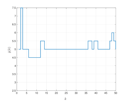
Figure 2: Filter output for a single simulation. Note that $\hat{y}(k)$ assumes a finite set of rational values, and hence satisfies conditions of Corollary 8.

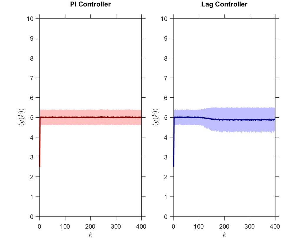
Figure 3: The solid curves represent the mean $y(k)$ over 2000 Monte Carlo simulations. The shaded areas denote one standard deviation around the mean. Regulation is observed (on average) for both the PI and for the lag controllers, within a given precision and for $x_{c}(0)=50$.

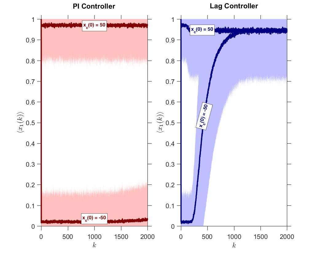
Figure 4: The solid curves represent the mean $x_{1}(k)$ over 2000 Monte Carlo simulations. The shaded areas denote one standard deviation around the mean. Four cases are considered in this figure, as we simulate the behaviour of $x_{1}$ for both controllers and two initial states, $x_{c}(0)=50$ and $x_{c}(0)=-50$. Predictability is lost for the PI controller but is satisfied for the lag controller, as $x_{c}(0)$ does not affect $\langle x_{1}(k)\rangle$ for the second controller on the long run.

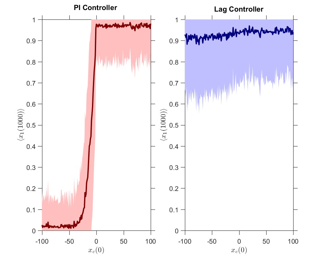
Figure 5: The solid curves represent the mean $x_{1}(1000)$ over 2000 Monte Carlo simulations. The shaded areas denote one standard deviation around the mean. This figure presents the behaviour of the average of $x_{1}(1000)$ for both controllers in dependence of the initial controller state $x_{c}(0)$. Predictability of $x_{1}(1000)$ is once again lost, when the PI controller is used.

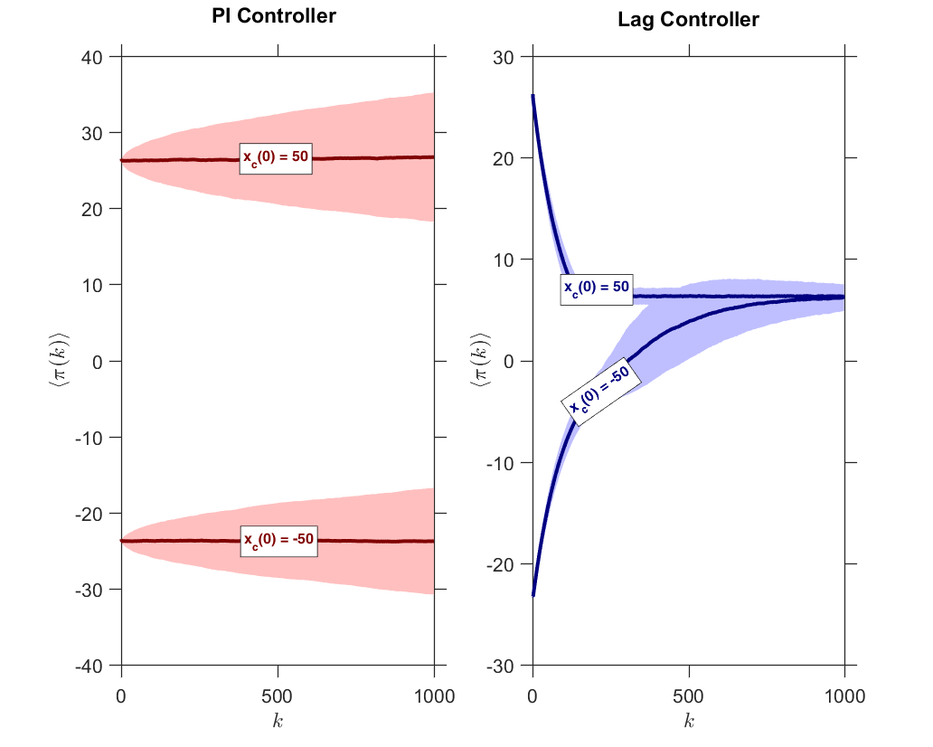
Figure 6: The solid curves represent the mean $\pi(k)$ over 2000 Monte Carlo simulations. The shaded areas denote one standard deviation around the mean. Four cases are considered in this figure: we consider both controllers for the simulations as well as two initial conditions, $x_{c}(0)=50$ and $x_{c}(0)=-50$, for each of them. Once again, predictability is lost for the PI controller, as observed by changing $x_{c}(0)$.

3.2 Positive Results: Ergodic Behaviour under Feedback

Finally, to conclude this section, we note that coupling fails in our PI example due to a lack of contractivity. Fortunately, for linear systems, the notion of contractivity needed for unique ergodicity is relatively easy to enforce, and we shall now provide conditions which guarantee a stable behavior, for particular combinations of agent dynamics, filter, and controller. Specifically, in the linear setting, the controller dynamics are:

$${\mathscr{C}}~{}:~{}\left\{\begin{array}[]{rcl}x_{c}(k+1)&=&A_{c}x_{c}(k)+B_{c}e(k),\vspace{0.1cm}\\ \pi(k)&=&C_{c}x_{c}(k)+D_{c}e(k),\end{array}\right.$$ (12)

where $x_{c}\in\mathbb{R}^{n_{c}}$ is the internal state of the controller of dimension $n_{c}$. We adopt a linear model for the $n_{f}$-dimensional filter ${\mathscr{F}}$, based on the classic IIR/FIR structures (Oppenheim et al., 1999). Remembering that $y$ is the sum of each agents’ output (as in Figure 1), one has

$${\mathscr{F}}~{}:~{}\left\{\begin{array}[]{rcl}x_{f}(k+1)&=&A_{f}x_{f}(k)+B_{f}y(k),\vspace{0.1cm}\\ \hat{y}(k)&=&C_{f}x_{f}(k).\end{array}\right.$$ (13)

Finally, to be consistent with our discussion we consider populations of agents whose dynamics are described by:

$${\mathscr{S}}_{i}~{}:~{}\left\{\begin{array}[]{rcl}x_{i}(k+1)&=&A_{i}x_{i}(k)+b_{i},\vspace{0.1cm}\\ y_{i}(k)&=&c_{i}^{T}x_{i}(k)+d_{i},\end{array}\right.$$ (14)

where $A_{i}\in\mathbb{R}^{n_{i}\times n_{i}}$, $c_{i}\in\mathbb{R}^{n_{i}}$. The inputs $b_{i}$ and $d_{i}$ are random variables that take values in $\mathbb{R}^{n_{i}}$ and $\mathbb{R}$, respectively, with $\mathbb{P}(b_{i}=b_{ij})=p_{ij}(\pi)$ and $\mathbb{P}(d_{i}={d}_{ij})=p_{ij}^{\prime}(\pi)$. Note that this is a generalisation of the situation when agents switch between two states on, off. The following result gives conditions for unique ergodicity.

Theorem 12.

Consider the feedback system depicted in Figure 1, with ${\mathscr{C}}$ and ${\mathscr{F}}$ given in (12) and (13). Assume that each agent $i\in\{1,\cdots,N\}$ has state $x_{i}$ with dynamics governed by the affine stochastic difference equations given in (14), where $A_{i}$ are Schur matrices and $b_{i}$ and $d_{i}$ are chosen, at each time step, from the sets $\{b_{ij}\}\subset\mathbb{R}^{n_{i}}$ and $\{d_{i\ell}\}\subset\mathbb{R}$ according to Dini continuous probability functions $p_{ij}(\cdot)$, respectively $p^{\prime}_{i\ell}(\cdot)$, that verify (4). Assume furthermore that there are scalars $\delta,\delta^{\prime}>0$ such that $p_{ij}(\pi)\geq\delta>0$, $p^{\prime}_{ij}(\pi)\geq\delta^{\prime}>0$ for all $(i,j)$ and all $\pi\in\Pi$. Then, for every stable linear controller $\mathscr{C}$ and every stable linear filter $\mathscr{F}$ compatible with the system structure, the feedback loop converges in distribution to a unique invariant measure.

Following (Barnsley et al., 1988), the proof is centred at the construction of an iterated function system (IFS) with place-(state-)dependent probabilities that describes the feedback system. To this end, consider the augmented state $\xi\mathrel{\mathop{:}}=[x^{T}~{},~{}x_{f}^{T}~{},~{}x_{c}^{T}]^{T}\in\mathbb{X}$, whose dynamic behaviour is described by the difference equation

$$\xi(k+1)={\mathscr{W}}_{\ell}(x)\mathrel{\mathop{:}}=\mathscr{A}\xi(k)+\beta_{\ell},$$ (15)

where

$$\mathscr{A}\mathrel{\mathop{:}}=\begin{bmatrix}\hat{A}&0&0\\ B_{f}{\bf 1}^{T}\hat{C}&A_{f}&0\\ 0&-B_{c}C_{f}&A_{c}\end{bmatrix}$$ (16)

where $\mathbf{1}$ is the vector of ones, $\hat{A}\mathrel{\mathop{:}}=\mathbf{diag}(A_{i})$, $\hat{C}\mathrel{\mathop{:}}=\mathbf{diag}(c_{i}^{T})$ and $\beta_{\ell}$ is built from all the combinations of the vectors $b_{ij}$, the scalars ${d}_{ij}$ and other signals. To apply Corollary 2.3 from (Barnsley et al., 1988), two observations must be made. First, note that each map ${\mathscr{W}}_{\ell}$ is chosen with probability $p_{\ell}(\pi)\geq\prod_{i=1}^{N}\delta_{i}>0$ and thus these probabilities are bounded away from zero. Second, since $\sigma({\mathscr{A}})=\sigma(\hat{A})\cup\sigma(A_{f})\cup\sigma(A_{c})$ and, by hypothesis, $A_{i}$, $A_{f}$ and $A_{c}$ are Schur matrices, for any induced matrix norm there exists $m\in\mathbb{N}$ sufficiently large such that $\|{\mathscr{A}}^{m}\|<1$. This provides the required average contractivity after $m$ steps. The result then follows from (Barnsley et al., 1988). The proof is complete.

Remark 13.

Dini’s condition on the probabilities may be replaced by simpler, more conservative assumptions, such as Lipschitz or Hölder conditions (Barnsley et al., 1988). Also the requirement $p_{ij}(\pi)\geq\delta_{i}>0$ in the theorem statement is not an artefact of our analysis, as $p_{ij}(\pi)=0$ may lead to a non-ergodic behaviour.

Remark 14.

As we have stressed in Remark 3, the existence of an attractive invariant measure is only a baseline ergodic property. Under mild but technical additional assumptions, it is possible to prove a geometric rate of convergence (Steinsaltz, 1999). Under further assumptions, one can prove results concerning the “shape” of the unique invariant measure, where it exists, such as moment bounds (Walkden, 2007). These would complement the present theorem.

Remark 15.

In Theorem 12, we assume that the feedback loop only consists of stable systems. This assumption may seem quite restrictive, but as shown in the examples, even marginal stability in one of its parts may lead to completely unpredictable results. As the result from (Barnsley et al., 1988) only requires contractivity on average, more general results are possible, but beyond the scope of the present paper. We also point out that each agent may have a local stabilising controller, as we are analysing the feedback loop from a macroscopic level.

4 Extensions: Non-linear systems and discrete action spaces

Considering that Theorem 2 does not require linearity, it is clear that one can extend its use to non-linear systems under suitable assumptions.

4.1 Non-linear controllers

A particular case of the general setup described in Figure 1 is given by systems of the following form:

$$\left\{\begin{array}[]{ccl}x_{i}(k+1)&\in&\{{\mathscr{W}}_{ij}(x_{i}(k))\;|\;j=1,\ldots,w_{i}\}\\ y_{i}(k)&\in&\{{\mathscr{H}}_{ij}(x_{i}(k))\;|\;j=1,\ldots,h_{i}\},\\ \end{array}\right.$$ (19)

$$\hskip 45.52458pty(k)=\sum_{i=1}^{N}y_{i}(k),$$ (20)

$${\mathscr{F}}~{}:~{}\left\{\begin{array}[]{ccl}x_{f}(k+1)&=&{\mathscr{W}}_{f}(x_{f}(k),y(k))\\ \hat{y}(k)&=&{\mathscr{H}}_{f}(x_{f}(k),y(k)),\end{array}\right.$$ (21)

$${\mathscr{C}}~{}:~{}\left\{\begin{array}[]{ccl}x_{c}(k+1)&=&{\mathscr{W}}_{c}(x_{c}(k),\hat{y}(k),r)\\ \pi(k)&=&{\mathscr{H}}_{c}(x_{c}(k),\hat{y}(k),r),\end{array}\right.$$ (22)

In addition, we have Dini continuous probability functions $p_{ij},p^{\prime}_{il}:\Pi\to[0,1]$ so that the probabilistic laws (4) are satisfied. If we denote by $\mathbb{X}_{i},i=1,\ldots,N,\mathbb{X}_{C}$ and $\mathbb{X}_{F}$ the state spaces of the agents, the controller and the filter, then the system evolves on the overall state space $\mathbb{X}:=\prod_{i=1}^{N}\mathbb{X}_{i}\times\mathbb{X}_{C}\times\mathbb{X}_{F}$ according to the dynamics

$$x(k+1):=\begin{pmatrix}(x_{i})_{i=1}^{N}\\ x_{f}\\ x_{c}\end{pmatrix}(k+1)\in\{F_{m}(x(k))\,|\,m\in{\mathbb{M}}\}.$$ (23)

where each of the maps $F_{m}$ is of the form

$$F_{m}(x(k))\mathrel{\mathop{:}}=\begin{pmatrix}({\mathscr{W}}_{ij}(x_{i}(k)))_{i=1}^{N}\\ {\mathscr{W}}_{f}(x_{f}(k),\sum_{i=1}^{N}{\mathscr{H}}_{i\ell}(x_{i}(k)))\\ {\mathscr{W}}_{c}(x_{c}(k),{\mathscr{H}}_{f}(x_{f}(k),\sum_{i=1}^{N}{\mathscr{H}}_{i\ell}(x_{i}(k))))\end{pmatrix}$$ (24)

and the maps $F_{m}$ are indexed by indices $m$ from the set

$$\mathbb{M}\mathrel{\mathop{:}}=\prod_{i=1}^{N}\{(i,1),\ldots,(i,w_{i})\}\times\prod_{i=1}^{N}\{(i,1),\ldots,(i,h_{i})\}.$$ (25)

By the independence assumption on the choice of the transition maps and output maps for the agents, for each multi-index $m=((1,j_{1}),\ldots,(N,j_{N}),(1,l_{1}),\ldots,(N,l_{N}))$ in this set, the probability of choosing the corresponding map $F_{m}$ is given by

$$\mathbb{P}\left(x(k+1)=F_{m}(x(k))\right)=\\ \left(\prod_{i=1}^{N}p_{ij_{i}}(\pi(k))\right)\left(\prod_{i=1}^{N}p^{\prime}_{il_{i}}(\pi(k))\right)=:q_{m}(\pi(k)).$$ (26)

Theorem 16.

Consider the feedback system depicted in Figure 1. Assume that each agent $i\in\{1,\cdots,N\}$ has a state governed by the non-linear iterated function system

$$x_{i}(k+1) ={\mathscr{W}}_{ij}(x_{i}(k))$$ (27)

$$y_{i}(k) ={\mathscr{H}}_{ij}(x_{i}(k)),$$ (28)

where ${\mathscr{W}}_{ij}$ and ${\mathscr{H}}_{ij}$ are globally Lipschitz-continuous functions with global Lipschitz constant $l_{ij}$, resp. $l^{\prime}_{ij}$. Assume we have Dini continuous probability functions $p_{ij},p^{\prime}_{il}$ so that the probabilistic laws (4) are satisfied. Assume furthermore that there are scalars $\delta,\delta^{\prime}>0$ such that $p_{ij}(\pi)\geq\delta>0$, $p^{\prime}_{ij}(\pi)\geq\delta^{\prime}>0$ for all $(i,j)$. Further, assume that the following contractivity condition holds: for all $1\leq i\leq N,1\leq j\leq J$: $l_{ij}<1$. Then, for every stable linear controller $\mathscr{C}$ and every stable linear filter $\mathscr{F}$ compatible with the feedback structure, the feedback loop has a unique attractive invariant measure. In particular, the system is uniquely ergodic.

Similarly to the proof of Theorem 12 the assumptions on the Lipschitz constants and the the internal asymptotic stability of controller and filter guarantees that suitable iterates of the maps $F_{m}$ are strict contractions. The result then follows again from Theorem 2.1 and Corollary 2.2 of (Barnsley et al., 1988).

Remark 17.

Notice that Lipschitz continuity can be rephrased in many ways. For instance, there is the QUAD condition (DeLellis et al., 2011), the sector condition, or, when restricting to convex functions, the bounded subgradient condition. The sector condition requires that there exist constants $c_{1}$ and $c_{2}$ such that the vector-valued functions ${\mathscr{W}}(x):=[{\mathscr{W}}_{i}(x)]$ and ${\mathscr{H}}(x):=[{\mathscr{H}}_{i}(x)]$ satisfy ${\mathscr{W}}(x)^{T}[{\mathscr{W}}(x)-c_{1}x]\leq 0$ and ${\mathscr{H}}(x)^{T}[{\mathscr{H}}(x)-c_{2}x]\leq 0$. The bounded subgradient condition requires the existence of constants $c_{3},c_{4}$, such that for a given norm $|\cdot|$, for all $z,z^{\prime}$ in the subdifferentials of ${\mathscr{W}},{\mathscr{H}}$, respectively, at all points in the domains of the respective functions, we have that $|z|\leq c_{3},|z^{\prime}|\leq c_{4}$. Here the functions ${\mathscr{W}}(x)$, ${\mathscr{H}}(x)$ are assumed to be convex with a non-empty subdifferential throughout their domains, but not necessarily differentiable. The equivalence follows from basic convex analysis, e.g., as a corollary of Lemma 2.6 in (Shalev-Shwartz, 2012).

Let us refer back to Remark 3 for a discussion of the importance of unique ergodicity; notably, the existence of the limit (8) almost surely.

4.2 Discrete Action Spaces

Next, consider the case, when the agents’ actions are limited to a finite set. In this case the Lipschitz conditions in Theorem 16 cannot be satisfied except in trivial cases. In this case we may use results in (Werner, 2005, 2004) to obtain ergodicity results.

The general setup of the following result is that for each agent $i$ the set ${\mathbb{A}}_{i}$ is finite. Then, $\mathbb{X}_{S}:=\prod_{i=1}^{N}{\mathbb{A}}_{i}$ is finite and we consider the directed graph $G=(\mathbb{X}_{S},E)$, where there is an arc between vertices representing $(x_{i})\in\mathbb{X}_{S}$ and $(y_{i})\in\mathbb{X}_{S}$, if there is a choice of maps ${\mathscr{W}}_{ij}$ in (19) such that $({\mathscr{W}}_{ij}(x_{i}))=(y_{i})$.

Theorem 18.

Consider the feedback system depicted in Figure 1. Assume that ${\mathbb{A}}_{i}$ is finite for each $i$. Assume that each agent $i\in\{1,\ldots,N\}$ has a state governed by the non-linear stochastic difference equations (27). Assume we have Dini continuous probability functions $p_{ij},p^{\prime}_{il}$ so that the probabilistic laws (4) are satisfied. Assume furthermore that there are scalars $\delta,\delta^{\prime}>0$ such that $p_{ij}(\pi)\geq\delta>0$, $p^{\prime}_{ij}(\pi)\geq\delta^{\prime}>0$ for all $(i,j)$ and all $\pi$. Then, for every stable linear controller $\mathscr{C}$ and every stable linear filter $\mathscr{F}$ the following holds:

If the graph $G=(\mathbb{X}_{S},E)$ is strongly connected, then there exists an invariant measure for the feedback loop. If in addition, the adjacency matrix of the graph is primitive, then the invariant measure is attractive and the system is uniquely ergodic.

This is a consequence of (Werner, 2004) and the observation that the necessary contractivity properties follow from the internal asymptotic stability of controller and filter.

We note that a simple condition for the primitivity of the graph $G=(\mathbb{X}_{S},E)$ is that for each agent the graph describing the possible transitions is primitive.

Remark 19.

We note that there are a few cases, to which both Theorem 12 and Theorem 18 are applicable. Namely, if in the assumptions of Theorem 12 all $A_{i}=0$, then each agent at each time step chooses its next state $x_{i}(k+1)$ independently of the current state $x_{i}(k)$. In Theorem 18 this corresponds to the case that the ${\mathscr{W}}_{ij}$ are constant maps and the directed transition graph of the system is complete.

5 Conclusions and Further Work

Within feedback systems, the control of ensembles of agents presents a particularly challenging area for further study. Practically important examples of such systems arise in Smart Cities. Typically, such problems deviate from classical control problems in two main ways. First, even though ensembles are typically too large to allow for a microscopic approach, they are not sufficiently large to allow for a meaningful fluid (mean-field) approximation. Second, the regulation problem concerns not only the ensemble, but also the individual agents; a certain quality of service should be provided to each agent. We have formulated this problem as an iterated function system with the objective of designing an ergodic control, and demonstrated that controls with poles on the unit circle (e.g., PI) may destroy ergodicity even for benign ensembles.

This work was in part supported by Science Foundation Ireland grant 16/IA/4610, in part by Fundação de Amparo à Pesquisa do Estado de São Paulo (FAPESP) grants 2016/19504-7 and 2018/04905-1, in part by Conselho Nacional de Desenvolvimento Científico e Tecnológico (CNPq) grant 305600/2017-6 and in part by the European Union Horizon 2020 Programme (Horizon2020/2014-2020), under grant agreement no. 68838.

Appendix A An Overview of Notation

In general, our notation employs the following rules: Upper-case letters are used for matrices, (in caligraphic) groups, maps, operators, (and in blackboard) sets, and spaces, while lower-case letters are used for vectors, scalars, and functions. Subscripts are used to distinguish symbols; time-indexed symbols are followed by the time index in parentheses, as in $x(k)$. Superscript is used for exponentiation and, in ^T, for the transpose operation. Caligraphic fonts are used for maps and operators. Blackboard fonts are used for sets, spaces, and the probability operator $\mathbb{P}$. In particular, sets of real, rational, and natural numbers are indicated by $\mathbb{R}$, $\mathbb{Q}$, and $\mathbb{N}$, respectively. For a given space $\mathbb{X}$, $M(\mathbb{X})$ indicates the set of all probability measures over $\mathbb{X}$ and $\mathbb{X}^{\infty}$ denotes its associated path space, which consists of infinite right-sided sequences over $\mathbb{X}$.

In the following table of notations, we list related groups of symbols in the order of appearance; within each group of symbols, symbols are ordered alphabetically, Latin first and Greek second.

A Table of Notation
continues on next page
Symbol		Meaning
Standard sets:
$\mathbb{N}$	the set of natural numbers
$\mathbb{Q}$	the set of rational numbers
$\mathbb{R}$	the set of real numbers
Constants:
$\mathbf{1}$	a compatible vector of ones
$c_{1},\cdots,c_{4}$	constants used in Remark 17
$h_{i}$	the number of output maps ${\mathscr{H}}_{ij}$
$l_{ij}$	Lipschitz constant for a transition map
$l^{\prime}_{ij}$	Lipschitz constant for an output map
$N$	the number of agents
$n$	a dimension of a generic state space $\Sigma$
$n_{c}$	dimension of the state of the controller
$n_{f}$	dimension of the state of the filter
$n_{i}$	dimension of the state of $i$th agent’s private state
$m_{i}$	the number of possible actions of agent $i$
$m$	an upper bound on the number of possible actions of any agent
$r$	the reference value, i.e., desired value of $y(k)$
$\overline{r}_{i}$	$i$th agent’s expected share of the resource over the long run
$w_{i}$	the number of state transition maps ${\mathscr{W}}_{ij}$
$z$	${\mathscr{Z}}$-transform variable
$\alpha$	a constant used in the PI controller (9) or its lag approximant
$\beta$	a constant used in a lag controller
$\delta$	a constant in the iterated function system ergodicity used in Theorem 2
$\delta^{\prime}$	a constant in the iterated function system ergodicity used in Theorem 12
$\eta$	a lower bound on the values of probability functions
$\kappa$	a constant used in the PI controller (9) or its lag approximant
Blocks:
$\mathscr{C}$	controller representing the central authority
${\mathscr{F}}$	filter
$\mathscr{S}_{1}$, $\mathscr{S}_{2}$, …, $\mathscr{S}_{N}$	systems modelling agents
Maps and operators:
$f_{j}$	a generic map in a generic iterated function system
$g$	a generic function of (8)
${\mathscr{H}}_{ij}$	an output map
${\mathscr{H}}_{c}$	a map modelling the controller in (22)
${\mathscr{H}}_{f}$	a map modelling the filter in (21)
$P(x,\mathbb{G})$	a generic transition operator
$P$	a state-and-signal-to-state transition operator
$\mathscr{P}_{k}$	a measure-space-over-states-to-measure-space-over-states operator
$p_{j}$	a probability function of a generic iterated function system
$p_{ij}$	a probability function for the choice of agent $i$’s transition map
$p^{\prime}_{i\ell}$	a probability function for the choice of agent $i$’s output map
${\mathscr{W}}_{ij}$	transition maps
${\mathscr{W}}_{c}$	maps modelling the controller in (22)
${\mathscr{W}}_{f}$	maps modelling the filter in (21)
$\Phi^{(1)}$	projector from a measure over the product of the two path spaces to a single path space
$\Phi^{(2)}$	projector from a measure over the product of the two path spaces to a single path space
Deterministic matrices used in the definitions:
$A_{i}$	a matrix used in the agent dynamics (14) of Theorem 12
$A_{c}$	a matrix used in the controller (12) of Theorem 12
$A_{f}$	a matrix used in the filter (13) of Theorem 12
$B_{c}$	a matrix used in the controller (12) of Theorem 12 and in Theorem 6
$B_{f}$	a matrix used in the filter (13) of Theorem 12
$B_{i}$	a matrix used in the agent dynamics (14) of Theorem 12
$C_{c}$	a matrix used in the controller (12) of Theorem 12 and in Theorem 6
$C_{f}$	a matrix used in the filter (12) of Theorem 12
$c_{i}$	a vector used in the agent dynamics (14) of Theorem 12
$D_{c}$	a matrix used in the controller (12) of Theorem 12
$d_{i}$	a vector used in the agent dynamics (14) of Theorem 12
$X(k)$	element of a generic state space
$\{X(k)\}_{k\in\mathbb{N}}$	a generic Markov chain
Deterministic matrices and constants used in proofs:
$\mathscr{A}$	augmented state transition matrix in (16)
$\hat{A}$	$\mathbf{diag}(A_{i})$ in (16)
$\beta_{\ell}$	is built from all $b_{ij}$, ${d}_{ij}$, and other signals in (16)
$\hat{C}$	$\mathbf{diag}(c_{i}^{T})$ in (16)
$E$	edges of a graph in the proof of Theorem 18
$G$	a graph in the proof of Theorem 18
$K$	a constant used in the proof of Theorem 6
$Q$	a scalar or matrix used in the proof of Theorem 6
$R$	a marginally Schur matrix used in the proof of Theorem 6
Algebras, groups, sets, and spaces:
$\mathbb{A}_{i}$	the set of $i$th agent’s actions
${\mathbb{C}}$	set of couplings
$\mathbb{D}_{i}$	set of possible resource demands of agent $i$
$\mathbb{B}(\Sigma)$	Borel $\sigma$-algebra
${\mathscr{E}}$	a real additive group of Theorem 6
$\mathbb{G}$	a generic event
$\mathbb{H}$	a set used in the definition of asymptotic couplings
$\mathbb{J}$	index set of a generic iterated function system
${\mathbb{M}}$	an index set of (25)
$M(\mathbb{X})$	a measure-space over $\mathbb{X}$
$M(\mathbb{X}^{\infty})$	a measure space over the path space
${\mathbb{O}}_{\mathscr{F}}$	set of possible output values of the filter ${\mathscr{F}}$
$\bar{\mathbb{S}}$	a measurable subset of a state space
$\mathbb{X}_{i}$	a private state space of agent $i$, often $\mathbb{R}^{n_{i}}$
$\mathbb{X}_{S}$	a product space of state spaces of all agents
$\mathbb{X}_{F}$	a space of internal states of the filter
$\mathbb{X}_{C}$	a space of internal states of the central controller
$\mathbb{X}$	a state space of the controller, the filter, and the agents, combined
$\mathbb{X}^{\infty}$	a path space
${\mathbb{Z}}$	set used in the proof of Theorem 6
$\Pi$	the set of admissible broadcast control signals
$\Sigma$	a generic state space
Random variables:
$e(k)$	the error signal at time $k$, i.e., $\hat{y}(k)-r$
$\pi(k)$	the signal broadcast at time $k$
$x_{c}(k)$	the internal state of the controller at time $k$ of dimension $n_{c}$
$x_{f}(k)$	the internal state of the filter at time $k$ of dimension $n_{f}$
$x_{i}(k)$	the internal state of agent $i$ at time $k$
$y_{i}(k)$	the resource utilisation of agent $i$ at time $k$
$y(k)$	the aggregate resource utilisation at time $k$
$\hat{y}(k)$	the value of $y(k)$ filtered by filter $\mathscr{F}$
$\lambda$	initial state (distribution)
Further notation
$P_{\lambda}$	a probability measure induced on the path space
$\mu$	a generic measure, usually on state space $\Sigma$
$\Gamma$	a generic measure over the product of the two path spaces, potentially a coupling
$\nu$	a counter

References

- Alagoz et al. (2013) B. B. Alagoz, A. Kaygusuz, M. Akcin, and S. Alagoz. A closed-loop energy price controlling method for real-time energy balancing in a smart grid energy market. Energy, 59:95–104, 2013.
- Bárány (2015) B. Bárány. On iterated function systems with place-dependent probabilities. Proceedings of the American Mathematical Society, 143:419–432, 2015.
- Barnsley (2013) M. Barnsley. Fractals Everywhere: New Edition. Dover books on mathematics. Dover Publications, 2013. ISBN 9780486320342.
- Barnsley et al. (1988) M. Barnsley, S. Demko, J. Elton, and J. Geronimo. Invariant measures for Markov processes arising from iterated function systems with place-dependent probabilities. Annales de l’institut Henri Poincaré (B) Probabilités et Statistiques, 24(3):367–394, 1988.
- Barnsley et al. (1989) M. F. Barnsley, J. H. Elton, and D. P. Hardin. Recurrent iterated function systems. Constructive approximation, 5(1):3–31, 1989.
- Blondel et al. (2005) V. Blondel, J. Hendrickx, A. Olshevsky, and J. Tsitsiklis. Convergence in multiagent coordination, consensus, and flocking. In Proceedings of the 44th IEEE Conference on Decision and Control, and the European Control Conference 2005, pages 2996–3000, Seville, Spain, Dec. 2005.
- Branicky (1994) M. S. Branicky. Stability of switched and hybrid systems. In Proceedings of the 33rd IEEE Conference on Decision and Control, volume 4, pages 3498–3503 vol.4, Dec 1994.
- Branicky (1998) M. S. Branicky. Multiple Lyapunov functions and other analysis tools for switched and hybrid systems. IEEE Transactions on Automatic Control, 43(4):475–482, Apr 1998.
- Callaway and Hiskens (2011) D. S. Callaway and I. A. Hiskens. Achieving controllability of electric loads. Proceedings of the IEEE, 99(1):184–199, Jan 2011.
- Caves et al. (1988) D. W. Caves, J. A. Herriges, P. Hanser, and R. J. Windle. Load impact of interruptible and curtailable rate programs: evidence from ten utilities. IEEE Transactions on Power Systems, 3(4):1757–1763, Nov 1988.
- Chen and Cheng (2010) B. Chen and H. H. Cheng. A review of the applications of agent technology in traffic and transportation systems. IEEE Transactions on Intelligent Transportation Systems, 11(2):485–497, June 2010.
- Conejo et al. (2010) A. Conejo, J. Morales, and L. Baringo. Real-time demand response model. IEEE Transactions on Smart Grid, 1(3):236–242, Dec. 2010.
- Corless et al. (2016) M. Corless, C. King, R. Shorten, and F. Wirth. AIMD Dynamics and Distributed Resource Allocation. Advances in Design and Control. Society for Industrial and Applied Mathematics, 2016.
- DeLellis et al. (2011) P. DeLellis, M. di Bernardo, and G. Russo. On QUAD, Lipschitz, and contracting vector fields for consensus and synchronization of networks. IEEE Transactions on Circuits and Systems I: Regular Papers, 58(3):576–583, March 2011.
- Elton (1987) J. H. Elton. An ergodic theorem for iterated maps. Ergodic Theory and Dynamical Systems, 7(04):481–488, 1987.
- Epperlein and Marecek (2017) J. Epperlein and J. Marecek. Resource allocation with population dynamics. In 2017 55th Annual Allerton Conference on Communication, Control, and Computing (Allerton), pages 1293–1300, Oct 2017.
- Fioravanti et al. (2017) A. R. Fioravanti, J. Mareček, R. N. Shorten, M. Souza, and F. R. Wirth. On classical control and smart cities. In Proc. 2017 IEEE 56th Annual Conference on Decision and Control (CDC), pages 1413–1420, Dec 2017.
- Franklin et al. (1994) G. F. Franklin, J. D. Powell, and A. B. Emami-Naeini. Feedback Control of Dynamic Systems. Addison Wesley, Reading, MA, 1994.
- Franklin et al. (1997) G. F. Franklin, J. D. Powell, and M. L. Workman. Digital Control of Dynamic Systems. Prentice Hall, Englewood Cliffs, NJ, 3rd edition, 1997.
- Hairer (2006) M. Hairer. Ergodic properties of Markov processes. Warwick University lecture notes, 2006.
- Hairer et al. (2011) M. Hairer, J. C. Mattingly, and M. Scheutzow. Asymptotic coupling and a general form of Harris’ theorem with applications to stochastic delay equations. Probability Theory and Related Fields, 149(1-2):223–259, 2011.
- Harris (1960) T. E. Harris. A lower bound for the critical probability in a certain percolation process. Mathematical Proceedings of the Cambridge Philosophical Society, 56(1):13–20, 1960.
- Iosifescu (2009) M. Iosifescu. Iterated function systems: A critical survey. Mathematical Reports, 11(3):181–229, 2009.
- Lindvall (2012) T. Lindvall. Lectures on the Coupling Method. Dover Books on Mathematics. Dover Publications, 2012.
- Marecek et al. (2015) J. Marecek, R. Shorten, and J. Y. Yu. Signaling and obfuscation for congestion control. International Journal of Control, 88(10):2086–2096, 2015.
- Marecek et al. (2016) J. Marecek, R. Shorten, and J. Y. Yu. r-extreme signalling for congestion control. International Journal of Control, 89(10):1972–1984, 2016.
- Mathew and Mezić (2011) G. Mathew and I. Mezić. Metrics for ergodicity and design of ergodic dynamics for multi-agent systems. Physica D, 240:432–442, 2011. Physica D.
- McArthur et al. (2007) S. McArthur, E. Davidson, V. Catterson, A. Dimeas, N. Hatziargyriou, F. Ponci, and T. Funabashi. Multi-agent systems for power engineering applications — Part I: Concepts, approaches, and technical challenges. IEEE Transactions on Power Systems, 22(4):1743–1752, Nov. 2007.
- Mohsenian-Rad and Leon-Garcia (2010) A.-H. Mohsenian-Rad and A. Leon-Garcia. Optimal residential load control with price prediction in real-time electricity pricing environments. IEEE Transactions on Smart Grid, 1(2):120–133, Sept. 2010.
- Nedić and Ozdaglar (2009) A. Nedić and A. Ozdaglar. Distributed subgradient methods for multi-agent optimization. IEEE Transactions on Automatic Control, 54(1):48–61, Jan. 2009.
- Oppenheim et al. (1999) A. V. Oppenheim, R. W. Schafer, and J. R. Buck. Discrete-Time Signal Processing. Prentice-Hall, Upper Saddle River, USA, 2nd edition, 1999.
- Pillai and Bak-Jensen (2011) J. R. Pillai and B. Bak-Jensen. Integration of vehicle-to-grid in the western Danish power system. IEEE Transactions on Sustainable Energy, 2(1):12–19, Jan 2011.
- Salsbury et al. (2013) T. Salsbury, P. Mhaskar, and S. J. Qin. Predictive control methods to improve energy efficiency and reduce demand in buildings. Computers and Chemical Engineering, 51:77–85, 2013.
- Schlote et al. (2013) A. Schlote, F. Häusler, T. Hecker, A. Bergmann, E. Crisostomi, I. Radusch, and R. Shorten. Cooperative regulation and trading of emissions using plug-in hybrid vehicles. IEEE Transactions on Intelligent Transportation Systems, 14(4):1572–1585, 2013.
- Schlote et al. (2014) A. Schlote, C. King, E. Crisostomi, and R. Shorten. Delay-tolerant stochastic algorithms for parking space assignment. IEEE Transactions on Intelligent Transportation Systems, 15(5):1922–1935, Oct 2014.
- Shalev-Shwartz (2012) S. Shalev-Shwartz. Online learning and online convex optimization. Foundations and Trends® in Machine Learning, 4(2):107–194, 2012.
- Shaukat et al. (2018) N. Shaukat, B. Khan, S. Ali, C. Mehmood, J. Khan, U. Farid, M. Majid, S. Anwar, M. Jawad, and Z. Ullah. A survey on electric vehicle transportation within smart grid system. Renewable and Sustainable Energy Reviews, 81:1329–1349, 2018.
- Steinsaltz (1999) D. Steinsaltz. Locally contractive iterated function systems. Annals of Probability, 27(4):1952–1979, 1999.
- Stenflo (2001) Ö. Stenflo. Markov chains in random environments and random iterated function systems. Transactions of the American Mathematical Society, 353(9):3547–3562, 2001.
- Stenflo (2012) Ö. Stenflo. A survey of average contractive iterated function systems. Journal of Difference Equations and Applications, 18(8):1355–1380, 2012.
- Szarek (2003) T. Szarek. Invariant measures for Markov operators with application to function systems. Studia Math, 154(3):207–222, 2003.
- United States Federal Energy Regulatory Commission (2017) United States Federal Energy Regulatory Commission. Assessment of Demand Response and Advanced Metering: Staff Report. FERC, 2017.
- Walkden (2007) C. Walkden. Invariance principles for iterated maps that contract on average. Transactions of the American Mathematical Society, 359(3):1081–1097, 2007.
- Werner (2004) I. Werner. Ergodic theorem for contractive Markov systems. Nonlinearity, 17(6):2303–2313, 2004.
- Werner (2005) I. Werner. Contractive Markov systems. Journal of the London Mathematical Society, 71(1):236–258, 2005.
- Zanella et al. (2014) A. Zanella, N. Bui, A. Castellani, L. Vangelista, and M. Zorzi. Internet of things for smart cities. IEEE Internet of Things Journal, 1(1):22–32, 2014.