On U(1) Gauge Theory Transfer-Matrix in Fourier Basis
Narges Vadood       and     Amir H. Fatollahi 
Department of Physics, Alzahra University, Tehran 1993891167, Iran

Abstract

The properties of the transfer-matrix of U(1) lattice gauge theory in the Fourier basis are explored. Among other statements it is shown: 1) the transfer-matrix is block-diagonal, 2) all consisting vectors of a block are known based on an arbitrary block vector, 3) the ground-state belongs to the zero-mode’s block. The emergence of maximum-points in matrix-elements as functions of the gauge coupling is clarified. Based on explicit expressions for the matrix-elements we present numerical results as tests of our statements.

Keywords: Lattice gauge theories; Transfer-matrix method; Energy spectrum

1 Introduction

Currently the numerical studies of gauge theories in the non-perturabative regime are mainly based on the lattice formulation of these theories [1, 2, 3, 4]. The theoretical [5, 6, 7, 8, 9] as well as the numerical [10, 11, 12, 13, 14, 15, 16] studies suggest that the compact 4D U(1) gauge theory possesses two different phases, the so-called Coulomb and confined ones. Different studies suggest that the phase transition occurs at a critical coupling of order unity [5, 6, 7, 8, 9, 10, 11, 12, 13, 14, 15, 16].

The advantages of Fourier transform of lattice gauge variables have already been shown in the so-called dual formulation of the theory [5, 6], by which an insightful picture for the phases of U(1) theory is provided. Accordingly, in a certain small coupling limit known as Villain approximation [17] and via the Fourier basis, the partition function by the U(1) model looks like the one of monopoles or circulating-monopoles in 3D and 4D cases, respectively [5]. As a consequence, depending on temperature the system may exhibit different phases based on the spatial extent of the electric field out of an electric charge [5]. As other studies based on the dual formulation see [18, 19, 20].

In the present work the main concern is the transfer-matrix on its own as the basic tool to define the quantum theory on a Euclidean lattice [1, 2]. In particular, regarding the transfer-matrix in the Fourier basis, some mathematical statements are presented. The ultimate goal of studies in this direction is to provide more detailed information about the transfer-matrix based on the first principles of lattice gauge theories, leading to the better understanding of the energy spectrum of these models. Except the asymptotic behaviors of the matrix-elements, the statements are obtained with no use of approximation based on the value of gauge coupling, and are valid in any lattice size and dimension. The issues to be addressed include: the block-diagonal nature of matrix in the Fourier basis, the consisting vectors of each block, the small and large coupling limits of the matrix elements, and the block to which the ground-state belongs. Also the emergence of maximum-points in the matrix-elements as functions of gauge coupling is discussed and clarified. Based on the explicit form of matrix-elements for the 3D case as unconstrained summations, some pieces of numerical results are presented as the prompt test of the statements, all confirming the announced results.

The organization of the rest of the paper is as follows. In Sec. 2 the elements of the transfer-matrix are derived in the Fourier basis. In Sec. 3 the properties of the transfer-matrix and its elements in the Fourier basis are explored and formulated in six propositions. Also based on the properties a simplified expression for the matrix-elements are obtained which is more convenient for numerical purposes. In Sec. 4 the numerical results based on the obtained expression is presented as a demonstration for the practical use of the obtained expression as well as the tests of the statements. Sec. 5 is devoted to the conclusions.

2 Transfer-Matrix in Fourier Basis

The matrix element of the transfer-matrix $\widehat{V}$ between two adjacent times $n_{0}$ and $n_{0}+1$ is given by [21]

$$\langle n_{0}+1|\widehat{V}|n_{0}\rangle=\mathcal{A}~{}e^{S_{E}(n_{0},n_{0}+1)}$$ (1)

in which $\mathcal{A}$ is inserted to fix the normalization, and $S_{E}(n_{0},n_{0}+1)$ is the Euclidean action symmetrized in variables of two adjacent times. Following [22, 23, 24] here we work in the temporal gauge $A^{0}\equiv 0$, in which the transfer-matrix gets a particularly simple form. It is convenient to replace the gauge variables at adjacent times $A_{n_{0}}^{(\bm{r},i)}$ and $A_{n_{0}+1}^{(\bm{r},i)}$ on spatial link $(\bm{r},i)$ by the new angle variables [1]

$$\begin{aligned} \theta^{(\bm{r},i)}&=a\,g\,A_{n_{0}}^{(\bm{r},i)}\cr\theta^{\prime(\bm{r},i)}&=a\,g\,A_{n_{0}+1}^{(\bm{r},i)}\end{aligned}$$ (2)

both taking values in $[-\pi,\pi]$ [1]. In Eq. 2 $a$ and $g$ are the lattice spacing parameter and the gauge coupling, respectively. The symmetrized Euclidean action in Eq. 1 for pure U(1) theory in temporal gauge on a lattice with $d$ spatial dimensions is explicitly given by [23, 24]

$$S_{E}(n_{0},n_{0}+1)=-\frac{1}{2\,g^{2}}\sum_{\bm{r}}\sum_{i\neq j=1}^{d} \left[2-\cos\big{(}\theta^{(\bm{r},i)}+\theta^{(\bm{r}+\widehat{i},j)}-\theta^{(\bm{r}+\widehat{j},i)}-\theta^{(\bm{r},j)}\big{)}\right.$$ (3)

$$\left.-\cos\big{(}\theta^{\prime(\bm{r},i)}+\theta^{\prime(\bm{r}+\widehat{i},j)}-\theta^{\prime(\bm{r}+\widehat{j},i)}-\theta^{\prime(\bm{r},j)}\big{)}\right]$$ (4)

$$-\frac{1}{g^{2}} \sum_{\bm{r}}\sum_{i=1}^{d}\left[1-\cos\big{(}\theta^{(\bm{r},i)}-\theta^{\prime(\bm{r},i)}\big{)}\right]$$ (5)

in which $\widehat{i}$ is the unit-vector along the spatial direction $i$. For a spatial lattice with $N_{\mathrm{P}}$ plaquettes and $N_{\mathrm{L}}$ links, it is convenient to define the plaquette-link matrix $\bm{M}$ of dimension $N_{\mathrm{P}}\times N_{\mathrm{L}}$ given by

$$M^{p}_{~{}l}=\begin{cases}+1,&\mbox{link $l=(\bm{r},i)$ belongs to oriented plaquette $p$ }\\ -1,&\mbox{link $l=(\bm{r},-i)$ belongs to oriented plaquette $p$}\\ ~{}~{}0,&\mbox{otherwise.}\end{cases}$$ (6)

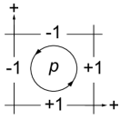
Figure 1: Graphical representation of definition (6).

In Fig. 1 the above definition is presented graphically. An explicit example for definition (6) in $d=2$ case will be given later. In terms of this matrix, labeling links as $l=(\bm{r},i)$ and plaquettes as $p$, the action (3) comes to the following form

$$S_{E}(n_{0},n_{0}+1)=-\frac{1}{2g^{2}}\sum_{p} \left[2-\cos\big{(}M^{p}_{~{}l}\,\theta^{l}\big{)}-\cos\big{(}M^{p}_{~{}l}\,\theta^{\prime l}\big{)}\right]$$ (7)

$$-\frac{1}{g^{2}}\sum_{l}\left[1-\cos\big{(}\theta^{l}-\theta^{\prime l}\big{)}\right]$$ (8)

in which summation over repeated indices is understood. Using

$$\gamma=\frac{1}{g^{2}}$$ (9)

and by Eq. (7) the matrix-element (1) may be written as

$$\langle\bm{\theta^{\prime}}|\widehat{V}|\bm{\theta}\rangle=~{}\mathcal{A}~{} \prod_{p}\exp\!\left\{-\frac{\gamma}{2}\left[2-\cos\big{(}M^{p}_{~{}l}\,\theta^{l}\big{)}-\cos\big{(}M^{p}_{~{}l}\,\theta^{\prime l}\big{)}\right]\right\}$$ (10)

$$\times\prod_{l}\exp\!\left\{-\gamma\Big{[}1-\cos\big{(}\theta^{l}-\theta^{\prime l}\big{)}\Big{]}\right\}$$ (11)

According to $\widehat{V}=\exp(-a\,\widehat{H})$, the eigenvalues $E_{i}$ of the Hamiltonian and $v_{i}$ of the transfer-matrix are related by

$$E_{i}=-\frac{1}{a}\ln v_{i}$$ (12)

As the main tool of this work, we formulate the theory in the Fourier basis $|k_{l}\rangle$, which is related to the compact $\theta$-basis by

$$\langle\theta^{l^{\prime}}|k_{l}\rangle =\frac{\delta^{l^{\prime}}_{~{}l}}{\sqrt{2\,\pi}}\,\exp(\mathrm{i}\,k_{l}\,\theta^{l}),~{}~{}~{}~{}~{}k_{l}=0,\pm 1,\pm 2,\cdots$$ (13)

Using the expansion

$$\exp(x\,\cos\phi)=\sum_{n}\mathrm{I}_{n}(x)\,\exp(\mathrm{i}\,n\,\phi)$$ (14)

for the modified Bessel functions $\mathrm{I}_{n}(x)$ of the first kind and the relation

$$\int_{-\pi}^{\pi}\mathrm{d}\theta\,\exp(\mathrm{i}\,n\,\theta)=2\pi\,\delta_{n,0}$$ (15)

one directly finds the matrix elements of $\widehat{V}$ in the field Fourier basis

$$\langle\bm{k}^{\prime}|\widehat{V}|\bm{k}\rangle=\mathcal{A}\,e^{-\gamma(N_{\mathrm{P}}+N_{\mathrm{L}})}\,(2\pi)^{N_{\mathrm{L}}}\sum_{\{n_{p}\}}\sum_{\{n^{\prime}_{p}\}}\prod_{p}\mathrm{I}_{n_{p}}\!\left(\frac{\gamma}{2}\right)\,\mathrm{I}_{n^{\prime}_{p}}\!\left(\frac{\gamma}{2}\right)\;\prod_{l}\mathrm{I}_{m_{l}}\!(\gamma)\,\delta_{m_{l},m^{\prime}_{l}},$$ (16)

with

$$m_{l}=k_{l}+\sum_{p}n_{p}\,M^{p}_{~{}l},~{}~{}~{}~{}~{}m^{\prime}_{l}=\,k^{\prime}_{l}-\sum_{p}n^{\prime}_{p}\,M^{p}_{~{}l}.$$ (17)

where $n_{p}$, $n^{\prime}_{p}$, $m_{l}$ and $m^{\prime}_{l}$ are all integer-valued.

3 Properties of Fourier Matrix-Element

The matrix-element (16) in the Fourier basis is the basis expression based on it in the following some propositions (by Pn’s) and their proofs (by Pf’s) are presented:

Pn $\bm{1}$: For every matrix element we have the following properties:
1) non-negativity: $\langle\bm{k}^{\prime}|\widehat{V}|\bm{k}\rangle\geq 0$, 2) symmetry: $\langle\bm{k}^{\prime}|\widehat{V}|\bm{k}\rangle=\langle\bm{k}|\widehat{V}|\bm{k}^{\prime}\rangle$, 3) reflectivity: $\langle\bm{k}^{\prime}|\widehat{V}|\bm{k}\rangle=\langle-\bm{k}^{\prime}|\widehat{V}|-\bm{k}\rangle$.

Pf $\bm{1}$: All of the above properties are evident using the properties $\mathrm{I}_{n}(x)\geq 0$ and $\mathrm{I}_{n}(x)=\mathrm{I}_{-n}(x)$, and appropriate sign-changes of the indices $n_{p}$, $n^{\prime}_{p}$ and $m_{l}$.

It is obvious that not only all matrix elements are non-negative, but also each term is so in the sum (16). The vanishing of a matrix element means that the difference $\bm{k}^{\prime}-\bm{k}$ can not satisfy all the Kronecker $\delta$’s in Eq. (16) for any set of integers $\{n_{p},n^{\prime}_{p}\}$.

Pn $\bm{2}$: All diagonal elements are non-zero: $\langle\bm{k}|\widehat{V}|\bm{k}\rangle\neq 0$.

Pf $\bm{2}$: It is easy to see that there are always surviving terms for $\bm{k}^{\prime}=\bm{k}$ in Eq. (16). On the diagonal $\bm{k}=\bm{k}^{\prime}$, setting all $n_{p}+n^{\prime}_{p}=0$ is enough to satisfy all $\delta$’s in Eq. (16), leading to non-vanishing positive terms.

In fact, for satisfying $\delta$’s in Eq. (16) with $\bm{k}=\bm{k}^{\prime}$, it is sufficient to set $n_{p}+n^{\prime}_{p}={n}^{0}_{p}$ with the condition $\sum_{p}{n}^{0}_{p}M^{p}_{~{}l}=0$, presented in the vector notation as

$$\bm{n}^{\bm{0}}\cdot\bm{M}=\bm{0}$$ (18)

Later we will give the general form of the non-zero elements based on the $\bm{n^{0}}$ vectors.

Pn $\bm{3}$: Transitivity: If $\langle\bm{k}|\widehat{V}|\bm{k}^{\prime}\rangle\neq 0$ and $\langle\bm{k}^{\prime}|\widehat{V}|\bm{k}^{\prime\prime}\rangle\neq 0$, then $\langle\bm{k}|\widehat{V}|\bm{k}^{\prime\prime}\rangle\neq 0$.

Pf $\bm{3}$: This simply follows by two successive uses of the $\delta$’s in Eq. (16).

By Pn 2 & 3, having a non-zero matrix element is an equivalence relation, by which the set of all $\bm{k}$’s is partitioned into equivalence classes. Later by explicit examples we will see that there is more than one class (in fact, an infinite number of classes) even for a finite size lattice. As a consequence, the transfer-matrix $\widehat{V}$ appears in the block-diagonal form based on the classes, with all elements of each block being non-zero. The remarkable fact is that, given by a Fourier mode $\bm{k}$ one can simply construct all of its co-blocks. This is simply done by setting $n_{p}+n^{\prime}_{p}=q_{p}+{n}^{0}_{p}$, in which $q_{p}$’s are arbitrary. Then by using $\sum_{p}{n}^{0}_{p}M^{p}_{~{}l}=0$ another mode in the class is obtained as $k^{\{q\}}_{l}=k_{l}‎+‎\sum_{p}q_{p}\,‎M^{p}_{~{}l}$,‎ presented in the vector notation by

$$\bm{k}^{\bm{q}}=\bm{k}+\bm{q}\cdot\bm{M}$$ (19)

It is obvious by definition (17) that the two modes $\bm{k}$ and $\bm{k}^{\bm{q}}$ satisfy all $\delta$’s in Eq. (16). Also if $\bm{q}$ satisfy the condition (18), the two modes are the same ($\bm{k}^{\bm{q}}=\bm{k}$). For two modes related by Eq. (19) the non-zero matrix-element simply gets the form

$$\langle\bm{k}^{\bm{q}}|\widehat{V}|\bm{k}\rangle=\mathcal{A}\,e^{-\gamma(N_{\mathrm{P}}+N_{\mathrm{L}})}\,(2\pi)^{N_{\mathrm{L}}} \sum_{\{{n}^{0}_{p}\}}\delta\Big{(}\sum_{p}{n}^{0}_{p}M^{p}_{~{}l}\Big{)}\sum_{\{n_{p}\}}$$ (20)

$$\prod_{p}\mathrm{I}_{n_{p}}\!\left(\frac{\gamma}{2}\right)\mathrm{I}_{q_{p}+{n}^{0}_{p}-n_{p}}\!\left(\frac{\gamma}{2}\right)\prod_{l}\mathrm{I}_{k_{l}+\sum_{p}\!\!n_{p}M^{p}_{~{}l}}\!(\gamma)$$ (21)

The important fact is that the allowed ${n}^{0}_{p}$’s are not depending on $\bm{k}$, but only on the matrix $\bm{M}$. As an instructive example, let us consider the case of a 2d periodic spatial lattice, for which we later explicitly find that the sub-space of the vectors $\bm{n^{0}}$ satisfying condition (18) is one-dimensional with the general form

$$\bm{n^{0}}=n^{0}\underbrace{(1,1,\cdots,1)}_{N_{\mathrm{P}}}=n^{0}\,\bm{s}$$ (22)

For periodic lattices with $d=2$ the matrix-element (20) gets the form

$$\langle\bm{k}^{\bm{q}}|\widehat{V}|\bm{k}\rangle=\mathcal{A}\,e^{-\gamma(N_{\mathrm{P}}+N_{\mathrm{L}})}(2\pi)^{N_{\mathrm{L}}}\sum_{{n}^{0}}\sum_{\{n_{p}\}} \prod_{p}\mathrm{I}_{n_{p}}\!\left(\frac{\gamma}{2}\right)\mathrm{I}_{q_{p}+{n}^{0}-n_{p}}\!\left(\frac{\gamma}{2}\right)$$ (23)

$$\prod_{l}\mathrm{I}_{k_{l}+\sum_{p}\!\!n_{p}M^{p}_{~{}l}}\!(\gamma)$$ (24)

This expression, with no restriction on summations, is quite adequate for numerical purposes and will be used later.

Pn $\bm{4}$: Each block of $\widehat{V}$ is infinite dimensional.

Pf $\bm{4}$: This simply follows by the infinite possible choices for the integer sets $\{q_{p}\}$’s.

For definiteness, throughout this work we consider the normalization $\mathcal{A}$ to be constant (i.e. independent of $g$); for other choices and their consequences see [25]. The limit $\gamma\ll 1$ (large coupling limit $g\gg 1$) of the matrix elements is obtained easily by the expansion of exponentials in Eq. (10), by which in the lowest orders one finds

$$\langle\bm{k}^{\prime}|\widehat{V}|\bm{k}\rangle =\mathcal{A}\,e^{-\gamma(N_{\mathrm{P}}+N_{\mathrm{L}})}\,(2\pi)^{N_{\mathrm{L}}}\,\bigg{\{}\prod_{l}\delta(k_{l})\,\delta(k^{\prime}_{l})$$ (25)

$$+\frac{\gamma}{4}\sum_{p}\bigg{[}\prod_{l}\delta\left(k_{l}+M^{p}_{~{}l}\right)\delta(k^{\prime}_{l})+\prod_{l}\delta\left(k_{l}-M^{p}_{~{}l}\right)\delta(k^{\prime}_{l})$$ (26)

$$~{}~{}~{}~{}~{}~{}+\prod_{l}\delta(k_{l})\delta\left(k^{\prime}_{l}-M^{p}_{~{}l}\right)+\prod_{l}\delta(k_{l})\delta\left(k^{\prime}_{l}+M^{p}_{~{}l}\right)\bigg{]}$$ (27)

$$+\frac{\gamma}{2}\bigg{[}\prod_{l}\delta(k_{l}+1)\,\delta(k^{\prime}_{l}-1)+\prod_{l}\delta(k_{l}-1)\,\delta(k^{\prime}_{l}+1)\bigg{]}+O(\gamma^{2})\bigg{\}}$$ (28)

This leads to the next important proposition:

Pn $\bm{5}$: Provided that the ground-state is unique, it belongs to the $\bm{k}=\mathbf{0}$ block.

Pf $\bm{5}$: According to expansion (25), in the $\gamma\to 0$ limit all the elements of $\widehat{V}$ are approaching zero, except the diagonal element $V_{\mathbf{00}}=\langle\mathbf{0}|\widehat{V}|\mathbf{0}\rangle$. By the relation (12) between energy eigenvalues and $\widehat{V}$-eigenvalues, all energies are going to infinity in limit $\gamma\to 0$ except the one in $V_{\mathbf{00}}$’s block, appearing as the lowest energy. Since lowering the coupling (increasing $\gamma$) does not cause a mixing among the blocks, by the uniqueness assumption, the ground-state belongs to the $\bm{k}=\mathbf{0}$’s block at any coupling.

The other interesting limit is at $\gamma\to\infty$ ($g\to 0$), which is expected to recover the ordinary formulation of the gauge theory in the continuum. This limit can be reached by using the asymptotic behavior of Bessel functions for large arguments. They read in the saddle-point approximation

$$\mathrm{I}_{n}(x)\simeq\frac{e^{x}}{\sqrt{2\pi x}}\,e^{-n^{2}/2x+1/8x}\,\big{(}1+\mathrm{O}(1/x^{2})\big{)},~{}~{}~{}~{}x\to\infty$$ (29)

by which in the $\gamma\to\infty$ limit the terms in the matrix-element (23) can be treated as Gaussian integrals, leading to the asymptotic behavior

$$\langle\bm{k}^{\bm{q}}|\widehat{V}|\bm{k}\rangle\simeq\mathcal{A}~{}\frac{(2\pi)^{\frac{1}{2}(N_{\mathrm{L}}+N_{\mathrm{P}})}}{\pi^{N_{\mathrm{P}}-\frac{1}{2}}\sqrt{\det\bm{C}}}\frac{1}{\sqrt{\bm{s}^{T}\!\bm{D}\bm{s}}}~{}\frac{e^{-B(\bm{k},\bm{q})/\gamma}}{\gamma^{\frac{1}{2}(N_{\mathrm{P}}+N_{\mathrm{L}}-1)}}\,e^{b/\gamma}$$ (30)

in which $b=(4N_{\mathrm{P}}+N_{\mathrm{L}})/8$, and $B(\bm{k},\bm{q})$, in terms of the symmetric matrices $\bm{C}$, $\bm{D}$ and $\bm{F}$, is

$$B(\bm{k},\bm{q})=\bm{q}^{T}\!\bm{D}\bm{q}+\frac{1}{2}\bm{k}^{T}\!\bm{F}\bm{k}+2\bm{q}^{T}\!\bm{C}^{-1}\!\bm{M}\bm{k}-\frac{\big{[}\bm{s}^{T}\!(\bm{D}\bm{q}+\bm{C}^{-1}\!\bm{M}\bm{k})\big{]}^{2}}{\bm{s}^{T}\!\bm{D}\bm{s}}$$ (31)

with $\bm{s}$ given in Eq. (22), and

$$\bm{C} =4\,\mathbb{1}_{N_{\mathrm{P}}}+\bm{M}\bm{M}^{T}\!,~{}~{}\bm{D}=\mathbb{1}_{N_{\mathrm{P}}}-2\,\bm{C}^{-1}\!,~{}~{}\bm{F}=\mathbb{1}_{N_{\mathrm{L}}}-\bm{M}^{T}\!\bm{C}^{-1}\!\bm{M}$$ (32)

in which $\mathbb{1}_{N}$ is the identity matrix of dimension $N$. For spatial lattices with dimensions larger than two, taking the dimension of sub-space of vectors $\bm{n^{0}}$ as $N_{0}$, the asymptotic behavior again can be obtained as $\langle\bm{k}^{\bm{q}}|\widehat{V}|\bm{k}\rangle\propto e^{\alpha/\gamma}/\gamma^{\frac{1}{2}(N_{\mathrm{P}}+N_{\mathrm{L}}-N_{0})}$, by which or by (30) the matrix-elements tend to zero by $\gamma\to\infty$ in any dimension. On the other hand by expansion (25), we already know that only $V_{\mathbf{00}}$ may survive in the limit $\gamma\to 0$. An immediate conclusion is:

Pn $\bm{6}$: Except perhaps $V_{\mathbf{00}}$, all non-zero matrix-elements are to develop maximum.

Pf $\bm{6}$: As by Pn 1 all non-zero matrix elements are positive, for the mentioned elements the increasing behavior at small $\gamma$ and the decreasing one at large $\gamma$ are to be connected through at least one maximum.

Our numerical results demonstrate clearly the appearance of precisely one maximum. The existence of the maximum in matrix elements of $\widehat{V}$ has particularly important consequences on the phases of the model; an issue that we do not discuss further and leave for later works.

4 Numerical Results

In this section examples of numerical results are presented based on the expressions obtained in the Fourier basis. The aim for presenting the numerical results is twofold. First to show how the final expressions in the Fourier basis, such as Eq. (23) can be used practically for generating numerical results. Second is to provide the tests for the statements presented in previous section, including the vectors belonging to a common block, and the appearances of maximum-points in the matrix elements.

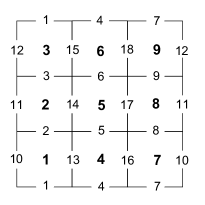
Figure 2: The numbering of links and plaquettes for the $3\times 3$ periodic lattice used in representation of matrix $\bm{M}$ (48).

To proceed let us have an explicit representation of the plaquette-link matrix $\bm{M}$. In the following we consider a lattice with two spatial dimensions $d=2$. For a 2-dim cubic periodic lattice with $N_{s}$ sites in each direction, it is convenient to define the $N_{s}\times N_{s}$ translation-matrix $\bm{T}$ by

$$T_{ab}=\delta_{ab}-\delta_{a+1,b}-\delta_{a,N_{s}}\,\delta_{b1},~{}~{}~{}~{}~{}a,b=1,\cdots,N_{s}$$ (33)

For $N_{s}=3$ the explicit form of $\bm{T}$ is

$$\bm{T}=\begin{pmatrix}+&-&0\cr 0&+&-\cr-&0&+\end{pmatrix}$$ (34)

For $N_{s}$ sites in each direction of a 2-dim periodic cubic lattice there are $N_{\mathrm{P}}=N_{s}^{2}$ plaquettes and $N_{\mathrm{L}}=2N_{s}^{2}$ links. Then, by the numbering of plaquettes and links as shown in Fig. 2, it is easy to check that the matrix $\bm{M}$ can be constructed by gluing the two $N_{s}^{2}\times N_{s}^{2}$ matrices next to each other, as follows

$$\bm{M}=\left(\begin{array}[]{c|c}&\cr\mathbb{1}_{N_{s}}\otimes\bm{T}{}&-\bm{T}\otimes\mathbb{1}_{N_{s}}\cr&\end{array}\right)$$ (38)

By construction, the matrix $\bm{M}$ is the $N_{s}^{2}\times 2N_{s}^{2}$ dimensional, as it should. For $N_{s}=3$ the matrix gets the form

$$\bm{M}=\left(\begin{array}[]{c@{\shrink}c@{\shrink}c@{\shrink}c@{\shrink} c@{\shrink}c@{\shrink}c@{\shrink}c@{\shrink}c@{\shrink\shrink} c@{\shrink}c@{\shrink}c@{\shrink}c@{\shrink}c@{\shrink}c@{\shrink} c@{\shrink}c@{\shrink}c}+\hfil\hskip 3.99994pt&-\hfil\hskip 3.99994pt&0\hfil\hskip 3.99994pt&0\hfil\hskip 3.99994pt&0\hfil\hskip 3.99994pt&0\hfil\hskip 3.99994pt&0\hfil\hskip 3.99994pt&0\hfil\hskip 3.99994pt&0\hfil\hskip 3.99994pt\hskip 3.99994pt&-\hfil\hskip 3.99994pt&0\hfil\hskip 3.99994pt&0\hfil\hskip 3.99994pt&+\hfil\hskip 3.99994pt&0\hfil\hskip 3.99994pt&0\hfil\hskip 3.99994pt&0\hfil\hskip 3.99994pt&0\hfil\hskip 3.99994pt&0\\ 0\hfil\hskip 3.99994pt&+\hfil\hskip 3.99994pt&-\hfil\hskip 3.99994pt&0\hfil\hskip 3.99994pt&0\hfil\hskip 3.99994pt&0\hfil\hskip 3.99994pt&0\hfil\hskip 3.99994pt&0\hfil\hskip 3.99994pt&0\hfil\hskip 3.99994pt\hskip 3.99994pt&0\hfil\hskip 3.99994pt&-\hfil\hskip 3.99994pt&0\hfil\hskip 3.99994pt&0\hfil\hskip 3.99994pt&+\hfil\hskip 3.99994pt&0\hfil\hskip 3.99994pt&0\hfil\hskip 3.99994pt&0\hfil\hskip 3.99994pt&0\\ -\hfil\hskip 3.99994pt&0\hfil\hskip 3.99994pt&+\hfil\hskip 3.99994pt&0\hfil\hskip 3.99994pt&0\hfil\hskip 3.99994pt&0\hfil\hskip 3.99994pt&0\hfil\hskip 3.99994pt&0\hfil\hskip 3.99994pt&0\hfil\hskip 3.99994pt\hskip 3.99994pt&0\hfil\hskip 3.99994pt&0\hfil\hskip 3.99994pt&-\hfil\hskip 3.99994pt&0\hfil\hskip 3.99994pt&0\hfil\hskip 3.99994pt&+\hfil\hskip 3.99994pt&0\hfil\hskip 3.99994pt&0\hfil\hskip 3.99994pt&0\\ 0\hfil\hskip 3.99994pt&0\hfil\hskip 3.99994pt&0\hfil\hskip 3.99994pt&+\hfil\hskip 3.99994pt&-\hfil\hskip 3.99994pt&0\hfil\hskip 3.99994pt&0\hfil\hskip 3.99994pt&0\hfil\hskip 3.99994pt&0\hfil\hskip 3.99994pt\hskip 3.99994pt&0\hfil\hskip 3.99994pt&0\hfil\hskip 3.99994pt&0\hfil\hskip 3.99994pt&-\hfil\hskip 3.99994pt&0\hfil\hskip 3.99994pt&0\hfil\hskip 3.99994pt&+\hfil\hskip 3.99994pt&0\hfil\hskip 3.99994pt&0\\ 0\hfil\hskip 3.99994pt&0\hfil\hskip 3.99994pt&0\hfil\hskip 3.99994pt&0\hfil\hskip 3.99994pt&+\hfil\hskip 3.99994pt&-\hfil\hskip 3.99994pt&0\hfil\hskip 3.99994pt&0\hfil\hskip 3.99994pt&0\hfil\hskip 3.99994pt\hskip 3.99994pt&0\hfil\hskip 3.99994pt&0\hfil\hskip 3.99994pt&0\hfil\hskip 3.99994pt&0\hfil\hskip 3.99994pt&-\hfil\hskip 3.99994pt&0\hfil\hskip 3.99994pt&0\hfil\hskip 3.99994pt&+\hfil\hskip 3.99994pt&0\\ 0\hfil\hskip 3.99994pt&0\hfil\hskip 3.99994pt&0\hfil\hskip 3.99994pt&-\hfil\hskip 3.99994pt&0\hfil\hskip 3.99994pt&+\hfil\hskip 3.99994pt&0\hfil\hskip 3.99994pt&0\hfil\hskip 3.99994pt&0\hfil\hskip 3.99994pt\hskip 3.99994pt&0\hfil\hskip 3.99994pt&0\hfil\hskip 3.99994pt&0\hfil\hskip 3.99994pt&0\hfil\hskip 3.99994pt&0\hfil\hskip 3.99994pt&-\hfil\hskip 3.99994pt&0\hfil\hskip 3.99994pt&0\hfil\hskip 3.99994pt&+\\ 0\hfil\hskip 3.99994pt&0\hfil\hskip 3.99994pt&0\hfil\hskip 3.99994pt&0\hfil\hskip 3.99994pt&0\hfil\hskip 3.99994pt&0\hfil\hskip 3.99994pt&+\hfil\hskip 3.99994pt&-\hfil\hskip 3.99994pt&0\hfil\hskip 3.99994pt\hskip 3.99994pt&+\hfil\hskip 3.99994pt&0\hfil\hskip 3.99994pt&0\hfil\hskip 3.99994pt&0\hfil\hskip 3.99994pt&0\hfil\hskip 3.99994pt&0\hfil\hskip 3.99994pt&-\hfil\hskip 3.99994pt&0\hfil\hskip 3.99994pt&0\\ 0\hfil\hskip 3.99994pt&0\hfil\hskip 3.99994pt&0\hfil\hskip 3.99994pt&0\hfil\hskip 3.99994pt&0\hfil\hskip 3.99994pt&0\hfil\hskip 3.99994pt&0\hfil\hskip 3.99994pt&+\hfil\hskip 3.99994pt&-\hfil\hskip 3.99994pt\hskip 3.99994pt&0\hfil\hskip 3.99994pt&+\hfil\hskip 3.99994pt&0\hfil\hskip 3.99994pt&0\hfil\hskip 3.99994pt&0\hfil\hskip 3.99994pt&0\hfil\hskip 3.99994pt&0\hfil\hskip 3.99994pt&-\hfil\hskip 3.99994pt&0\\ \makebox[0.0pt][l]{$\smash{\underbrace{\phantom{\begin{matrix}0&0&0&0&0&0&-&\end{matrix}}}_{\text{$\mathbb{1}_{3}\otimes\bm{T}$}}}$}0\hfil\hskip 3.99994pt&0\hfil\hskip 3.99994pt&0\hfil\hskip 3.99994pt&0\hfil\hskip 3.99994pt&0\hfil\hskip 3.99994pt&0\hfil\hskip 3.99994pt&-\hfil\hskip 3.99994pt&0\hfil\hskip 3.99994pt&+\hfil\hskip 3.99994pt\hskip 3.99994pt&\makebox[0.0pt][l]{$\smash{\underbrace{\phantom{\begin{matrix}0&0&+&0&0&0&0&\end{matrix}}}_{\text{$-\bm{T}\otimes\mathbb{1}_{3}$}}}$}0\hfil\hskip 3.99994pt&0\hfil\hskip 3.99994pt&+\hfil\hskip 3.99994pt&0\hfil\hskip 3.99994pt&0\hfil\hskip 3.99994pt&0\hfil\hskip 3.99994pt&0\hfil\hskip 3.99994pt&0\hfil\hskip 3.99994pt&-\\ \end{array}\right)$$ (48)

As announced before Eq. (22), it is an obvious consequence of this explicit form of $\bm{M}$ that the sub-space of $\bm{n^{0}}$ of Eq. (22) is one-dimensional. As two vectors in an equivalence class consider the followings

$$|\bm{0}\rangle \to\bm{k}=(0,0,\cdots,0)$$ (49)

$$|\bm{1}\rangle \to\bm{k^{q_{1}}}=\bm{q_{1}}\cdot\bm{M}$$ (50)

in which $\bm{q_{1}}=(1,0,\cdots,0)$ with $N_{\mathrm{P}}=N_{s}^{2}$ elements. By expansion (25) and Pn 5, the non-vanishing elements $V_{\bm{00}}$, $V_{\bm{01}}=V_{\bm{10}}$, and $V_{\bm{11}}$ belong to the ground-state’s block. To see how a vanishing element may occur, consider

$$|\bm{1^{\prime}}\rangle \to\bm{k_{1^{\prime}}}=(1,0,0,\cdots,0)$$ (51)

$$|\bm{1^{\prime\prime}}\rangle \to\bm{k_{1^{\prime\prime}}}=(0,1,0,\cdots,0)$$ (52)

$$|\bm{2}\rangle \to\bm{k_{2}}=(2,0,0,\cdots,0)$$ (53)

By an explicit representation like matrix (48), it is seen that any pair of the above vectors can not satisfy Eq. (19), leading to vanishing elements $V_{\bm{1^{\prime}1^{\prime\prime}}}=V_{\bm{1^{\prime\prime}2}}=V_{\bm{1^{\prime}2}}=0$. In other words, by the given representation for $\bm{M}$ and by any pair of Eqs. (51)-(53) one can see there is no solution for the $\{n_{p}+n^{\prime}_{p}\}$’s inside the $\delta$’s of Eq. (16). The same is true between each of Eqs. (51)-(53) and one of Eqs. (49)-(50). Hence, the five vectors (49)-(53) belong to four different blocks.

Using the explicit form of $\bm{M}$, the expression (23) with summations on $N_{s}^{2}+1$ integers in 2-dim case is quite adequate for numerical purposes. In the following to provide a prompt test for the announced results some pieces of numerical results are presented. The first issue in doing the summations is about a suitable choice of cut-off (upper limit) for sums. For small $\gamma$ limit we have

$$\mathrm{I}_{s}(\gamma)\simeq\frac{1}{s!}\left(\frac{\gamma}{2}\right)^{|s|},~{}~{}~{}~{}\gamma\ll|s|$$ (54)

by which for small arguments the Bessel’s of low degrees are quite dominant. The subtle point is about large arguments, for which an initial guess of cut-off is $s_{*}\simeq\sqrt{2}\,\gamma$, at which by behavior (29) we have $\mathrm{I}_{s_{*}}(\gamma)\propto 1/\sqrt{\gamma}$. However, in practice a lower cut-off is sufficient, as in the summations there are multiple of Bessel functions rather than a single one, making the convergence to the desired significant digits faster. As examples in the vacuum class the numerical evaluations of elements $V_{\bm{00}}$, $V_{\bm{01}}$, and $V_{\bm{11}}$ of modes (49) and (50) are presented in Fig. 3, by the choice $\mathcal{A}=1$ and for $3\times 3$ and $10\times 10$ lattices. To see how the statements work in the non-vacuum classes the elements $V_{\bm{1^{\prime}1^{\prime}}}=V_{\bm{1^{\prime\prime}1^{\prime\prime}}}$ and $V_{\bm{22}}$ are presented in Fig. 4; as mentioned $V_{\bm{1^{\prime}1^{\prime\prime}}}=V_{\bm{1^{\prime\prime}2}}=V_{\bm{1^{\prime}2}}=0$ since the modes belong to different classes. The results are generated on a desktop PC in reasonable time. Also the evaluated elements confirm numerically the announced asymptotic behavior (30). As expected by Pn 6, except $V_{\bm{00}}$ all other elements develop maximum.

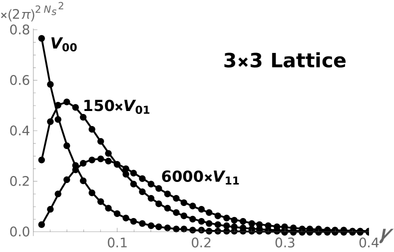
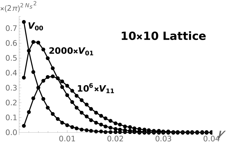
Figure 3: The elements $V_{\bm{00}}$, $V_{\bm{01}}$, and $V_{\bm{11}}$ in vacuum class versus $\gamma$ by (23) for normalization $\mathcal{A}=1$ for 2-dim lattices with $N_{s}=3$ and $N_{s}=10$.

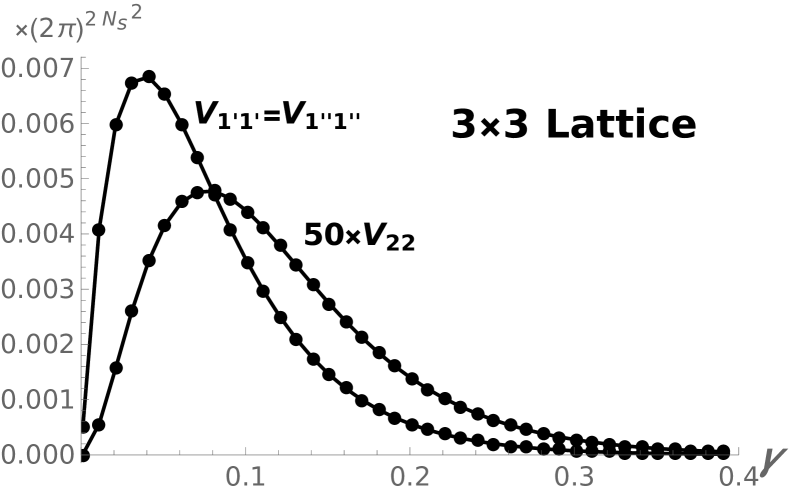
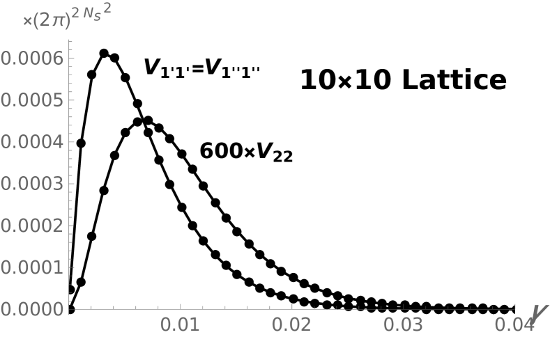
Figure 4: The elements $V_{\bm{1^{\prime}1^{\prime}}}=V_{\bm{1^{\prime\prime}1^{\prime\prime}}}$ and $V_{\bm{22}}$ (all in different blocks) versus $\gamma$ by Eq. (23) for normalization $\mathcal{A}=1$ for 2-dim lattices with $N_{s}=3$ and $N_{s}=10$.

5 Conclusion

In summary, in the present work we explored the properties of the transfer matrix in the Fourier basis for the U(1) lattice gauge theory. Regarding this matrix in the Fourier basis, some mathematical statements are presented, covering the issues: the block-diagonal nature of the matrix, the consisting vectors of each block, the small and large coupling limits of the matrix elements, the block to which the ground-state belongs, and the appearance of maximum in the elements as functions of coupling. Based on the explicit form of matrix-elements Eq. (23) for the 3D case, samples of numerical results are presented all in agreement with the announced properties. Apart from the asymptotic behaviors, the statements are obtained with no use of approximation based on the value of gauge coupling, and are valid in any lattice size and dimension. It is a matter of importance to see how the formalism based on the transfer-matrix in the Fourier basis regenerate the expected phase structures by the 3D and the 4D models [5], specially in a quantitative way. In particular, one of the main questions in this direction is what features of the phase structure by the pure U(1) model on lattice would survive in the continuum limit. This and further analytical and numerical results in this direction will be presented in future.

Acknowledgment: The authors are grateful to M. Khorrami for helpful discussions. This work is supported by the Research Council of the Alzahra University.

References

[1] K.G. Wilson,
Phys. Rev. D 10 (1974) 2445.
[2] J.B. Kogut,
Rev. Mod. Phys. 51 (1979) 659.
[3] H.J. Rothe, “Lattice Gauge Theories: An Introduction”,
World Scientific 2012.
[4] T. DeGrand and C. DeTar, “Lattice Methods for Quantum Chromodynamics”,
World Scientific 2006.
[5] T. Banks, R. Myerson, and J.B. Kogut,
Nucl. Phys. B 129 (1977) 493.
[6] R. Savit,
Phys. Rev. Lett. 39 (1977) 55.
[7] A.H. Guth,
Phys. Rev. D 21 (1980) 2291.
[8] J. Frohlich and T. Spencer,
Comm. Math. Phys. 83 (1982), 411-454.
[9] J. Glimm and A. Jaffe,
Comm. Math. Phys. 56 (1977) 195.
[10] G. Arnold, B. Bunk, Th. Lippert, K. Schilling,
Nucl. Phys. B: Proc. Supp. 119 (2003) 864,
0210010[hep-lat].
[11] K. Langfeld, B. Lucini, and A. Rago,
Phys. Rev. Lett. 109 (2012) 111601, 1204.3243[hep-lat]
[12] M. Creutz, L. Jacobs, and C. Rebbi,
Phys. Rept. 95 (1983) 201.
[13] B. Lautrup and M. Nauenberg,
Phys. Lett. B 95 (1980) 63–66.
[14] G. Bhanot,
Phys. Rev. D 24 (1981) 461.
[15] K.J.M. Moriarty,
Phys. Rev. D 25 (1982) 2185.
[16] T.A. DeGrand and D. Toussaint,
Phys. Rev. D 22 (1980) 2478.
[17] J. Villain,
J. Phys. (France) 36 (1975) 581.
[18] M. Zach, M. Faber, and P. Skala,
Phys. Rev. D 57 (1998) 123-131.
[19] M. Zach, M. Faber, and P. Skala,
Nucl. Phys. B 529 (1998) 505-522.
[20] M. Panero,
JHEP 0505 (2005) 066.
[21] A. Wipf, “Statistical Approach to Quantum Field Theory”,
Springer 2013, Sec. 8.5.1.
[22] M. Creutz, Phys. Rev. D 15 (1977) 1128
[23] M. Luscher,
Commun. Math. Phys. 54 (1977) 283-292.
[24] K. Osterwalder and E. Seiler,
Annals of Physics 110 (1978) 440-471.
[25] N. Vadood and A.H. Fatollahi,
“On Significance of Transfer-Matrix Normalization in Lattice Gauge Theories”,
1803.05497[hep-lat];
A.H. Fatollahi,
Eur. Phys. J. C 77 (2017) 159,
1611.08009[hep-th].