Compact stars in $f(T)$ extended theory of gravity

Abstract

We consider static spherically symmetric self-gravitating configurations of the perfect fluid within the framework of the torsion-based extended theory of gravity. In particular, we use the covariant formulation of $f(T)$ gravity with $f(T)=T+\frac{\alpha}{2}T^{2}$, and for the fluid we assume the polytropic equation of state with the adiabatic exponent $\Gamma=2$. The constructed solutions have a sharply defined radius [as in General Relativity (GR)] and can be considered as models of nonrotating compact stars. The particle number–to–stellar radius curves reveal that with positive (negative) values of $\alpha$ smaller (greater) number of particles can be supported against gravity then in GR. For the interpretation of the energy density and the pressure within the star we adopt the GR picture where the effects due to nonlinearity of $f(T)$ are seen as a $f(T)$ fluid, which together with the polytropic fluid contributes to the effective energy momentum. We find that sufficiently large positive $\alpha$ gives rise to an abrupt sign change (phase transition) in the energy density and in the principal pressures of the $f(T)$ fluid, taking place within the interior of the star. The corresponding radial profile of the effective energy density is approximately constant over the central region of the star, mimicking an incompressible core. This interesting phenomenon is not found in configurations with negative $\alpha$.

1 Introduction

Since the early days of General Relativity (GR), it has been known that replacing the Ricci scalar $R$ in the Einstein-Hilbert action with the torsion scalar $T$ yields a theory of gravity of which the equations of motion are equivalent to those of GR. The torsion-based variant of the theory is known as the teleparallel equivalent of General Relativity [1]. However, if the gravitational action is extended by allowing for terms of the form $f(R)$ or $f(T)$, where $f$ is a nonlinear function, the resulting curvature-based and torsion-based extended theories of gravity become grossly different. The curvature-based $f(R)$ gravity has been thoroughly studied over the past decades [2]. Its most remarkable feature is the occurrence of fourth order derivatives of the metric in the resulting equations of motion. In contrast to this, the equations of motion of the torsion-based $f(T)$ theory involve only the usual second order derivatives of the tetrad fields. The features of $f(T)$ theory have been widely studied in the cosmological setting, see e.g., Refs. [3, 4, 5, 6, 7, 8, 9, 10], and some constraints on the theory have been determined through considerations of the motion of planets in the Solar System, see e.g., Refs. [11, 12, 13], while investigations in the arena of static spherical symmetry, in particular those considering stellar structure, are somewhat fewer in number [14, 15, 16, 17, 18, 19, 20, 21] The structure of the theory itself has also been investigated [22, 23]. An important problem that was found in the early formulations of the $f(T)$ theory is the lack of the Lorentz invariance in the sense that the equations of motion are in general not invariant with respect to the choice of the metric compatible tetrad; see e.g., Refs. [24, 25]. In recent years, a lot of effort has been invested into understanding and solving this problem. Some of the promising results are in the form of the Hamiltonian formalism [26], the null tetrad approach [27], the Lagrange multiplier formulation [28, 29], and the covariant formulation [30, 31, 32]. In this work, we will rely on the covariant formulation of $f(T)$ gravity in the form proposed by Krššák and Saridakis in Ref. [30].

In GR, the models of nonrotating stars can be constructed within static spherical symmetry as solutions to the well-known Tolman-Oppenheimer-Volkov equations. One must also assume a matter model, which is often a perfect fluid subject to some equation of state. In general, the energy density and the pressure of the fluid may take up all space, while if they strictly vanish outside of a spherical surface of some finite radius, the models are said to represent compact stars surrounded by vacuum. Within GR, the phenomenology of these solutions is well understood. The most important results include proofs of existence of solutions with certain classes of equations of state [33, 34], upper bounds on the stellar mass–to–surface radius ratio that is also a measure of the “compactness” of a compact object [35, 36], as well as the relation among the stellar mass–to–surface radius curves and the dynamical stability of the models [37]. Our main goal in this paper is to obtain numerical evidence for the existence of similar solutions within the torsion-based extended theory of gravity. We intend to construct an analog of the stellar mass–to–radius curves of GR and search for possible signatures of the extended theory in the solutions. We will use the simplest possible variant of the $f(T)$ theory where the nonlinear function $f$ involves a term which is quadratic in $T$ [this variant of $f(T)$ can be seen as an analog of the Starobinsky $f(R)$ model in curvature-based theory [38], which has also become known as the $R^{2}$-gravity theory]. For the equation of state of the fluid, we adopt the polytropic equation of state with the adiabatic exponent $\Gamma=2$, since it represents the most stiff model of matter which satisfies the most important physical constraints in all pressure regimes.

The paper is organized as follows. In Sec. 2 we briefly review the equations of motion of the covariant $f(T)$ theory in static spherical symmetry. In Sec. 3 we introduce the polytropic equation of state, and in Sec. 4 we discuss the rescaling of the equations, the boundary conditions that we impose, and the numerical procedure. In Secs. 5 and 6, we discuss the particle number–to–stellar radius curves and the radial profiles of the energy density and the pressures. We conclude in Sec. 7. Geometrized units $c=1=G$ are used throughout the paper.

2 Static spherical symmetry in $f(T)$

The $f(T)$-gravity theory follows from the action written as

$$S=\int\left(\frac{f(T)}{16\pi}+\mathcal{L}_{\mathrm{matter}}\right)\det[h^{a}{}_{\mu}]\;\mathrm{d}^{4}x,$$ (1)

where $f$ is in general a nonlinear function of the torsion scalar $T$, $\mathcal{L}_{\mathrm{matter}}$ is the Lagrangian density due to matter fields, and $h^{a}{}_{\mu}$ is the tetrad, which is the dynamical degree of freedom of this theory. We use latin symbols for the tetrad indices and greek symbols for the spacetime indices. The tetrad satisfies the metric compatibility condition $h^{a}{}_{\mu}h^{b}{}_{\nu}g^{\mu\nu}=\eta^{ab}$, where $g^{\mu\nu}$ is the spacetime metric tensor and $\eta^{ab}$ is the Minkowski tensor. If $f(T)=T$, the resulting equations of motion are equivalent to those of GR, while if $f$ is nonlinear in $T$, the equation of motion can be written as [1, 30]

$$h^{-1}h^{a}{}_{\mu}\partial_{\sigma}\left(h\frac{\mathrm{d}f(T)}{\mathrm{d}T}S_{a}{}^{\nu\sigma}\right)-\frac{\mathrm{d}f(T)}{\mathrm{d}T}T_{\alpha\beta\mu}S^{\alpha\beta\nu}+\frac{1}{2}f(T)\delta_{\mu}{}^{\nu}+\frac{\mathrm{d}f(T)}{\mathrm{d}T}S_{a}{}^{\alpha\nu}h^{b}{}_{\mu}\omega^{a}{}_{b\alpha}=8\pi\mathcal{T}_{\mu}{}^{\nu}.$$ (2)

In the above equation, $\mathcal{T}_{\mu}{}^{\nu}$ is the usual energy-momentum tensor, and

$$T^{\alpha}{}_{\beta\gamma}=h_{a}{}^{\alpha}\left(\partial_{\beta}h^{a}{}_{\gamma}-\partial_{\gamma}h^{a}{}_{\beta}\right)+h_{a}{}^{\alpha}\omega^{a}{}_{b\beta}h^{b}{}_{\gamma}-h_{a}{}^{\alpha}\omega^{a}{}_{b\gamma}h^{b}{}_{\beta}$$ (3)

is the torsion tensor. The quantity $\omega^{a}{}_{b\alpha}$ is the inertial spin connection which is, in the covariant formulation of $f(T)$ gravity [30], determined from the requirement that the torsion tensor vanishes in the flat-space limit of the metric. The tensors

$$K_{\alpha\beta\gamma}=\frac{1}{2}\left(T_{\alpha\gamma\beta}+T_{\beta\alpha\gamma}+T_{\gamma\alpha\beta}\right)$$ (4)

and

$$S_{\alpha\beta\gamma}=K_{\beta\gamma\alpha}+g_{\alpha\beta}\,T_{\sigma\gamma}{}^{\sigma}-g_{\alpha\gamma}\,T_{\sigma\beta}{}^{\sigma}$$ (5)

are known as the contorsion tensor and the modified torsion tensor. The torsion scalar,

$$T=T^{\alpha\beta\gamma}S_{\alpha\beta\gamma},$$ (6)

is then defined as the contraction of the torsion tensor with the modified torsion tensor.

The specific form of $f(T)$ which we will be using is

$$f(T)=T+\frac{\alpha}{2}T^{2}.$$ (7)

With the above choice of $f(T)$, the left-hand side of the equation of motion (2) can be written as the sum of the Einstein tensor $G_{\mu}{}^{\nu}$ built from the Christoffel connection and the additional term proportional to $\alpha$ which we denote with the tilded symbol $\tilde{G}_{\mu}{}^{\nu}$. We then find it convenient to adopt the “GR picture” of the equation of motion by transferring $\tilde{G}_{\mu}{}^{\nu}$ to the right-hand side and writing the equation as

$$G_{\mu}{}^{\nu}=8\pi\left({\mathcal{T}}_{\mu}{}^{\nu}+\tilde{\mathcal{T}}_{\mu}{}^{\nu}\right),$$ (8)

where the quantity

$$\tilde{\mathcal{T}}_{\mu}{}^{\nu}=-\frac{1}{8\pi}\tilde{G}_{\mu}{}^{\nu}$$ (9)

can be interpreted as the contribution to the standard energy-momentum tensor arising from the nonlinear term in $f(T)$. We will refer to (9) as the energy-momentum tensor of the “$f(T)$ fluid”.

As we are intending to construct the models of static nonrotating stars, we now assume static spherical symmetry. We use spherical coordinates $x^{\mu}=(t,r,\vartheta,\varphi)$ and write the metric tensor as

$$g_{\mu\nu}=\mathrm{diag}\left(\mathrm{e}^{2\Phi(r)},-\mathrm{e}^{2\Lambda(r)},-r^{2},-r^{2}\sin^{2}\vartheta\right).$$ (10)

The tetrad compatible with the above metric can be chosen as

$$h^{a}{}_{\mu}=\mathrm{diag}\left(\mathrm{e}^{\Phi(r)},\mathrm{e}^{\Lambda(r)},r,r\sin\vartheta\right).$$ (11)

The condition that the torsion tensor (3) vanishes in the flat spacetime limit, which is obtained by letting $\Phi\to 0$ and $\Lambda\to 0$, gives the inertial spin connection of which the nonzero components are $\omega^{\hat{r}}{}_{\hat{\vartheta}\vartheta}=-\omega^{\hat{\vartheta}}{}_{\hat{r}\vartheta}=-1$, $\omega^{\hat{r}}{}_{\hat{\varphi}\varphi}=-\omega^{\hat{\varphi}}{}_{\hat{r}\varphi}=-\sin\vartheta$, and $\omega^{\hat{\vartheta}}{}_{\hat{\varphi}\varphi}=-\omega^{\hat{\varphi}}{}_{\hat{\vartheta}\varphi}=-\cos\vartheta$ (here, the coordinate labels are used as indices, and the tetrad indices are distinguished from the spacetime indices with the hat symbol). After lengthy but straightforward manipulations, one obtains the torsion scalar

$$T={2}{r^{-2}}\mathrm{e}^{-2\Lambda}\left(\mathrm{e}^{\Lambda}-1\right)\left(\mathrm{e}^{\Lambda}-2r\Phi^{\prime}-1\right),$$ (12)

where the prime denotes differentiation with respect to $r$. The nonzero components of the Einstein tensor are

$$G_{t}{}^{t} =r^{-2}\left(1-\mathrm{e}^{-2\Lambda}\left(1-2r\Lambda^{\prime}\right)\right),$$ (13)

$$G_{r}{}^{r} =r^{-2}\left(1-\mathrm{e}^{-2\Lambda}\left(1+2r\Phi^{\prime}\right)\right),$$ (14)

$$G_{\vartheta}{}^{\vartheta} =G_{\varphi}{}^{\varphi}=r^{-1}\mathrm{e}^{-2\Lambda}\left(\left(\Lambda^{\prime}-\Phi^{\prime}\right)\left(1+r\Phi^{\prime}\right)-r\Phi^{\prime\prime}\right),$$ (15)

while the nonzero terms on the left-hand side of the equation of motion (2) that are proportional to $\alpha$ are given by somewhat more complicated expressions:

$$\tilde{G}_{t}{}^{t} =\alpha r^{-4}\mathrm{e}^{-4\Lambda}\left(\mathrm{e}^{\Lambda}-1\right)\big{(}4r\Lambda^{\prime}\left(3\left(\mathrm{e}^{\Lambda}-1\right)+2\left(\mathrm{e}^{\Lambda}-3\right)r\Phi^{\prime}\right)+$$

$$\qquad\left(\mathrm{e}^{\Lambda}-1\right)\left(\left(\mathrm{e}^{\Lambda}-1\right)\left(\mathrm{e}^{\Lambda}-5\right)-4r^{2}\left(\Phi^{\prime 2}+2\Phi^{\prime\prime}\right)\right)\big{)},$$ (16)

$$\tilde{G}_{r}{}^{r} =\alpha r^{-4}\mathrm{e}^{-4\Lambda}\left(\mathrm{e}^{\Lambda}-1\right)\left(\mathrm{e}^{\Lambda}-1-2r\Phi^{\prime}\right)\left(\left(\mathrm{e}^{\Lambda}-1\right)\left(\mathrm{e}^{\Lambda}+3\right)+2\left(\mathrm{e}^{\Lambda}-3\right)r\Phi^{\prime}\right),$$ (17)

$$\tilde{G}_{\vartheta}{}^{\vartheta} =\tilde{G}_{\varphi}{}^{\varphi}=\alpha r^{-4}\mathrm{e}^{-4\Lambda}\big{(}$$

$$\qquad 2r\Lambda^{\prime}\big{(}3\left(\mathrm{e}^{\Lambda}-1\right)^{2}+3\left(\mathrm{e}^{\Lambda}-1\right)\left(\mathrm{e}^{\Lambda}-3\right)r\Phi^{\prime}-2\left(2\mathrm{e}^{\Lambda}-3\right)r^{2}\Phi^{\prime 2}\big{)}-$$

$$\qquad\left(\mathrm{e}^{\Lambda}-1\right)\big{(}\left(\mathrm{e}^{\Lambda}-1\right)^{2}\left(\mathrm{e}^{\Lambda}+3\right)+2\big{(}3\left(\mathrm{e}^{\Lambda}-1\right)r^{2}\Phi^{\prime 2}-2r^{3}\Phi^{\prime 3}+$$

$$\qquad 3\left(\mathrm{e}^{\Lambda}-1\right)r^{2}\Phi^{\prime\prime}+\left(1+\mathrm{e}^{\Lambda}-2\mathrm{e}^{2\Lambda}-4r^{2}\Phi^{\prime\prime}\right)r\Phi^{\prime}\big{)}\big{)}\big{)}.$$ (18)

The standard energy-momentum tensor of the perfect fluid in the static spherical symmetry has the well-known diagonal form

$$\mathcal{T}_{\mu}{}^{\nu}=\mathrm{diag}(\rho,-p,-p,-p),$$ (19)

where $\rho$ is the energy density and $p$ is the isotropic pressure of the fluid. The complete equations of stellar structure can now be written as

$$G_{t}{}^{t}=8\pi(\rho+\tilde{\rho}),\qquad G_{r}{}^{r}=-8\pi(p+\tilde{p}),\qquad G_{\vartheta}{}^{\vartheta}=-8\pi(p+\tilde{q}),$$ (20)

where the quantities

$$\tilde{\rho}=-\frac{1}{8\pi}\tilde{G}_{t}{}^{t},\qquad\tilde{p}=\frac{1}{8\pi}\tilde{G}_{r}{}^{r},\qquad\tilde{q}=\frac{1}{8\pi}\tilde{G}_{\vartheta}{}^{\vartheta},$$ (21)

are the energy density, the radial, and the transverse pressure of the $f(T)$ fluid. It is also important to note that, while the quantities (21) vanish in the Minkowski spacetime, they are nonzero in the general Schwarzschild spacetime; i.e., the Schwarzschild metric is not a vacuum solution of the nonlinear $f(T)$ theory of gravity [39]. This means that at the surface of the star, where the components of the fluid energy-momentum tensor (19) vanish and where the interior metric joins the exterior vacuum metric, the quantities (21) may have nonzero values.

3 Equation of state of the polytropic fluid

The equation of state (EoS) of a perfect fluid is in general specified as the dependence of the fluid pressure $p$ on the particle number density $n$ and the entropy per particle $s$, i.e., by specifying the function $p=p(n,s)$. Assuming the isentropic flow of the fluid, the entropy per particle $s$ is constant, allowing one to write the EoS simply as $p=p(n)$. The so-called polytropic EoS follows form the assumption that the adiabatic exponent $\Gamma=\left({\partial\ln p}/{\partial\ln n}\right)_{s}$ is independent of the pressure. For the EoS of the form $p=p(n)$, this implies $\Gamma=({n}/{p})({\mathrm{d}p}/{\mathrm{d}n})$, which upon integration gives

$$p=kn^{\Gamma},$$ (22)

where $k$ is the integration constant. The energy density of the polytropic fluid can be obtained by invoking the first law of thermodynamics. For a fluid element of proper volume $V$, it can be expressed as $T\mathrm{d}(nsV)=\mathrm{d}(\rho V)+p\,\mathrm{d}V$; since the number of particles in $V$ is constant, we use $V\propto 1/n$; and since in the isentropic flow $s$ is constant, it implies

$$\frac{\mathrm{d}\rho}{\mathrm{d}n}=\frac{\rho+p}{n}=\frac{\rho+kn^{\Gamma}}{n}.$$ (23)

Upon integration, one obtains

$$\rho=mn+\frac{kn^{\Gamma}}{\Gamma-1},$$ (24)

where the integration constant $m$ can be recognized as the mass of a single particle. Using (22) and denoting $\kappa=mk^{-1/\Gamma}$, the above relation can also be written in the form

$$\rho=\kappa p^{1/\Gamma}+\frac{p}{\Gamma-1}$$ (25)

which is known as the polytropic EoS. The square of the speed of the sound waves, sometimes also referred to as the stiffness of the fluid, for the fluid obeying the EoS (25) is given by

$$c_{\mathrm{sound}}^{2}=\left(\frac{\partial p}{\partial\rho}\right)_{s}=\frac{\Gamma-1}{1+(1-1/\Gamma)\kappa p^{-(1-1/\Gamma)}}.$$ (26)

We see that $c_{\mathrm{sound}}^{2}$ is monotonically increasing with pressure and is bounded from above by $\Gamma-1$. This implies that the polytropic fluids with $\Gamma\leq 2$ are causal (sound propagates at subluminal speeds) at all pressures. It is also easy to show that the pressure–to–energy density ratio

$$\sigma=\frac{p}{\rho}=\frac{\Gamma-1}{1+(\Gamma-1)\kappa p^{-(1-1/\Gamma)}}$$ (27)

is bounded from above with $\Gamma-1$. This means that the dominant energy condition (DEC), which requires that $p<\rho$, is satisfied at all pressures if $\Gamma\leq 2$. The limiting case of the polytropic fluid with $\Gamma=2$ can be singled out as the maximally stiff model of matter capable of withstanding arbitrarily large pressures without violating the basic principles (causality and DEC). We will therefore use $\Gamma=2$ in our models of compact objects.

4 Numerical procedure

In principle, the system of three coupled ordinary differential equations (20), the EoS of the polytropic fluid (25), and the set of appropriate boundary conditions (to be discussed below) determine the structure of the polytropic star or polytrope in $f(T)=T+\frac{\alpha}{2}T^{2}$ gravity. The parameter space is four dimensional and the parameters can be chosen as $\kappa>0$ and $\Gamma>1$ appearing in the EoS, the value of the fluid pressure–to–energy density ratio at the center of the star $\sigma_{0}=p(0)/\rho(0)$, and the coefficient $\alpha$ of the quadratic term in $f(T)$. The variables to be solved for can be chosen as the metric profile functions $\Phi(r)$ and $\Lambda(r)$ and the fluid pressure profile function $p(r)$. However, some elementary transformations make the system more adequate for the numerical treatment. The parameters $\kappa$ and $\gamma$ allow one to define the parameter

$$\lambda=\kappa^{-\Gamma/2(\Gamma-1)}$$ (28)

which has the dimension of length and which can be used as the length scale for the problem. In this way, the dimension of the parameter space reduces by one, and we chose to work with three dimensionless parameters,

$$a=\lambda^{-2}\alpha,\qquad\Gamma,\qquad\sigma_{0}=p(0)/\rho(0).$$ (29)

For the variables to solve for, we chose the functions

$$\Phi^{\prime}(r),\qquad\Lambda(r),\qquad\sigma(r)=p(r)/\rho(r).$$ (30)

[Note that the function $\Phi(r)$ does not appear in the equations of stellar structure, which means that it is sufficient to solve for $\Phi^{\prime}(r)$.] The transformation of the system of equations is straightforward, but since the resulting expressions are rather cluttered, they are not shown explicitly.

The boundary conditions appropriate for the problem can be specified at the center of symmetry and at the surface of the star. At the center of symmetry, we require

$$\Phi^{\prime}(0)=0,\qquad\Lambda(0)=0,\qquad\sigma(0)=\sigma_{0}.$$ (31)

The surface of the star is defined as the hypersurface $r=R$ at which the energy density of the fluid vanishes and the interior spacetime joins with the vacuum exterior. The boundary condition reflecting this is $\sigma(R)=0$. However, as the value of $R$ is a priori unknown, $R$ must be treated as an eigenvalue of the problem. Technically, this is done by introducing the dimensionless radial coordinate $x=r/R$ which maps the problem onto the compact domain $x\in[0,1]$. The boundary condition at the stellar surface is then

$$\sigma(1)=0.$$ (32)

The eigenvalue $R$ is obtained through the numerical solution of the boundary value problem (we use the tool colsys [40]), and the validity of each converged solution is confirmed by means of the a posteriori initial value integration. We also made sure that the results we obtain within GR (for $a=0$) reproduce the results from the literature, e.g., Refs. [41, 42].

It should be noted that within the framework of the $f(T)$ gravity one cannot unambiguously compute the mass of the star. While in GR the mass of a compact (finite radius) star computed from $M=4\pi\int_{0}^{R}\rho r^{2}\,\mathrm{d}r$ coincides with the Arnowitt-Deser-Misner (ADM) [43] mass of the spacetime, in $f(T)$ gravity, this result is not known to hold. Within the nonlinear $f(T)$-gravity theory, as a robust measure of the amount of matter contained within a certain stellar configuration, one can use the total particle number $N$. It can be obtained by integrating the particle number density $n=\mathrm{d}N/\mathrm{d}V$ over the interior of the star. Writing the proper volume element as $\mathrm{d}V=4r^{2}\pi\mathrm{e}^{\Lambda(r)}\mathrm{d}r$, the particle number is given by

$$N=4\pi\int_{0}^{R}n(r)\mathrm{e}^{\Lambda(r)}r^{2}\,\mathrm{d}r,$$ (33)

where the particle number density $n(r)$ is to be expressed in terms of $\sigma(r)$.

5 Particle number-to-stellar radius curves

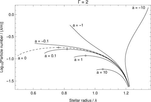
Figure 1: Particle number–to–stellar radius curves for polytropes with adiabatic exponent $\Gamma=2$ computed within GR ($a=0$, dashed line) and within the nonlinear $f(T)$-gravity theory ($a=\pm 0.1,\pm 1,\pm 10$, solid lines).

Table 1:

Parameters of some configurations of the $\Gamma=2$ polytropes computed within GR and within the nonlinear $f(T)$-gravity theory.

$a$	$\sigma_{0}$	$R/\lambda$	$N/(\lambda/m)$	$\mu(R)$	Comment
10	0.0369606	1.05013	0.0582413	0.117202	Critical
	0.0404008	1.01023	0.0561978	0.123072	Max. $\sigma_{0}$
1	0.0974466	0.938375	0.117965	0.296724	Critical
	0.117761	0.865438	0.108835	0.323215	Max. $\sigma_{0}$
0.1	0.187386	0.819034	0.164647	0.519582	Critical
	0.304203	0.673722	0.132935	0.604828	Max. $\sigma_{0}$
0 (GR)	0.241407	0.763518	0.179862	0.626006	Critical
-0.1	0.473319	0.609773	0.22232	0.906915	Max. $\sigma_{0}$
-1	0.451499	0.837695	0.575407	0.890173	Max. $\sigma_{0}$
-10	0.316375	1.34443	1.43548	0.644026	Max. $\sigma_{0}$

In General Relativity, a family of static spherically symmetric stellar models obtained with certain EoS and corresponding to a range of values of the central pressure–to–energy density ratio $\sigma_{0}$ is often represented by a curve on a mass–to–radius graph. The typical behavior of a mass–to–radius curve is such that as $\sigma_{0}$ increases starting from a sufficiently low value the radius of the star decreases, while the mass increases, reaches the maximum, and decreases with a further increase of $\sigma_{0}$. The configuration with maximal mass is usually called the critical configuration because it has been shown that all configurations with $\sigma_{0}$ lower than that corresponding to that configuration are stable with respect to small radial perturbations. If $\sigma_{0}$ increases beyond that critical value, the configurations become dynamically unstable. A similar pattern is found if instead of stellar mass $M$ one displays the particle number $N$ of the configuration. The dashed line in Fig. 1 shows the dependence of the particle number on the stellar radius for the GR ($a=0$) polytrope with $\Gamma=2$. Solid lines in Fig. 1 are the particle number–to–radius curves obtained with the same EoS, but within the nonlinear $f(T)$ theory with the coefficient $a=\pm 0.1,\pm 1,\pm 10$. All curves start at $\sigma_{0}=0.01$ and are continued only as far as the numerical procedure could obtain stable convergences. The critical configurations, in cases where they exist, are indicated by circle symbols. Precise values of the particle number and stellar radius for some of the solutions are given in Table 1. The table also contains the quantity $\mu(R)=1-\mathrm{e}^{-2\Lambda(R)}$, which is computed directly from the metric and which in GR corresponds to the ratio $2M/R$, where $M$ is the mass of the star. This quantity is usually taken as the measure of the compactness of the object and is bounded from above by unity.

We first note that as $\sigma_{0}\to 0$ solutions with all values of $a$ that we computed approach the nonrelativistic polytrope configuration described by the solution to the Lane-Emden equation with the polytropic index $n=1$ (see e.g., Ref. [44]). The stellar radius of this polytrope is $R=\sqrt{\pi/2}\,\lambda$.

For positive $a$, the particle number–to–radius curves that we obtained are qualitatively similar to the curve representing the GR solutions. In each of these curves, the critical configuration can be found. As $a$ increases, the radius of critical configuration increases, while the particle number decreases. This indicates that the amount of matter that can be supported against gravity with $a>0$ is less than in GR.

For negative $a$, if $|a|$ is sufficiently large, the particle number–to–radius curves may develop behavior which qualitatively differs from the behavior in GR. Starting from the nonrelativistic regime, as $\sigma_{0}$ increases, the particle number increases, but before the critical configuration is reached, the numerical procedure stops converging, indicating the lack of existence of solutions beyond that value of $\sigma_{0}$ (see the $a=-0.1$ or $a=-1$ curve in Fig. 1). With still larger values of $|a|$, the particle number–to–radius curves reveal configurations with the minimal radius, beyond which the radius starts to increase (see the $a=-10$ curve in Fig. 1). The critical points analogous to those that are typical for mass-to-radius curves in GR are no longer present in particle number–to–radius curves with sufficiently large negative parameter $a$. We also observe that, in comparison with the GR configurations, negative $a$ allows static configurations of much larger amounts of matter (number of particles) described by the same polytropic EoS. However, since we are not dealing with the full dynamic theory, nor with linearized dynamics of the system that would allow us to consider small perturbations, we are at present not able to make any claims regarding dynamical stability of any of the configurations computed within the nonlinear $f(T)$-gravity theory.

6 Energy density and pressure profiles

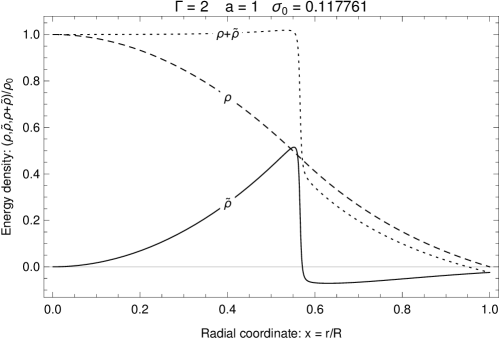
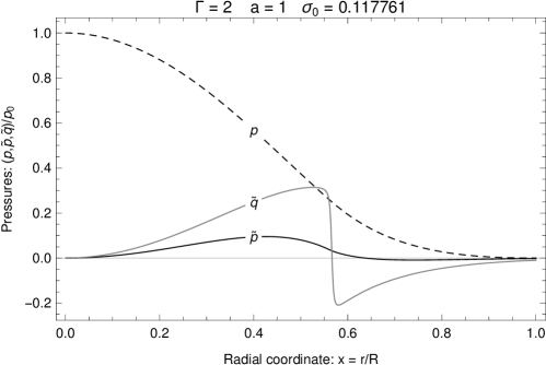
Figure 2: The $\Gamma=2$ polytrope (EoS $\rho=\kappa p^{1/2}+p$) with maximal $\sigma_{0}$ in $f(T)=T+\frac{\alpha}{2}T^{2}$-gravity theory, $a=\alpha\kappa^{2}=1$. Upper plot: energy density $\rho$ of the polytropic fluid (dashed line), energy density $\tilde{\rho}$ of the $f(T)$ fluid in the GR picture (solid line), and effective energy density $\rho+\tilde{\rho}$ (dotted line). Lower plot: isotropic pressure $p$ of the polytropic fluid (dashed line), radial pressure $\tilde{p}$ (solid black line), and transverse pressure $\tilde{q}$ (solid grey line) of the $f(T)$ fluid.

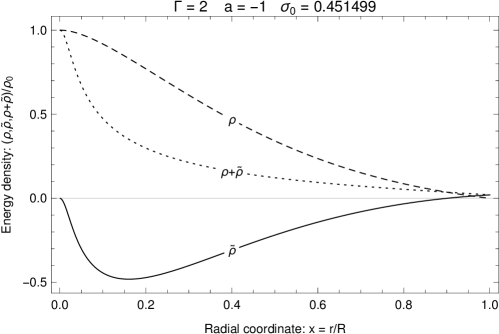
Figure 3: The $\Gamma=2$ polytrope with maximal $\sigma_{0}$ in $f(T)=T+\frac{\alpha}{2}T^{2}$-gravity theory, $a=\alpha\kappa^{2}=-1$. Energy density $\rho$ of the polytropic fluid (dashed line), energy density $\tilde{\rho}$ of the $f(T)$ fluid in the GR picture (solid line), and effective energy density $\rho+\tilde{\rho}$ (dotted line).

We begin by examining the energy density and the pressure profiles in the polytropes obtained with positive values of $a$. In all configurations, we find qualitative behavior of the polytropic fluid similar to that in GR; the fluid has outwardly decreasing energy density, and at some finite value of the radial coordinate $r=R$ corresponding to the stellar surface, it satisfies the boundary condition (32). This means that the energy density $\rho$ and the pressure $p$ of the polytropic fluid both vanish at the stellar surface. Using the GR picture allows us to examine also the energy density $\tilde{\rho}$, the radial pressure $\tilde{p}$, and the transverse pressure $\tilde{q}$ of the $f(T)$ fluid. All these quantities vanish at $r=0$ and are outwardly increasing (positive) in the central region of the polytrope. They reach their maxima in the interior of the polytrope after which they start to decrease, change sign, and remain negative until reaching the stellar surface. It is important to emphasize that at the stellar surface the quantities $\tilde{\rho}$, $\tilde{p}$, and $\tilde{q}$ assume finite negative values appropriate for joining the vacuum of the $f(T)$-gravity theory, which differs from the Schwarzschild vacuum of GR.

The energy density and the pressure profiles of the polytrope obtained with $\Gamma=2$, $a=1$, and with the maximal value of the central pressure–to–energy density ratio $\sigma_{0}\simeq 0.118$ that could be reached with our numerical procedure are shown in Fig. 2. One can observe a very abrupt transition of the $f(T)$ fluid energy density $\tilde{\rho}$ and the transverse pressure $\tilde{q}$ from their “positive phase” in the central region of the star to their “negative phase” in the outer region of the star, while the “phase transition” of the radial pressure $\tilde{p}$ is somewhat smoother. Comparing the configurations obtained with different values $a$ and maximal $\sigma_{0}$ that could be reached with our numerical procedures (corresponding to the upper ends of $N$ vs $R$ curves in Fig. 1 and with parameters given in Table 1) reveals that the phase transition becomes sharper as $a$ increases. However, as our results are obtained numerically, we cannot claim that a further increase of $\sigma_{0}$ is in principle possible and that it would lead to even more steplike phase transitions; nor can we claim with certainty that such solutions do not exist. Still, the results that we obtained with positive $a$ and high $\sigma_{0}$ allow us to loosely divide the interior of such polytropes into three regions: the core, the phase transition layer, and the halo. The core of the polytrope is its central region in which, within the GR picture, the energy density and pressures of the $f(T)$ fluid are positive and the effective energy density is approximately constant. This behavior of effective energy density $\rho+\tilde{\rho}$ mimics what could be understood as incompressible matter, i.e., matter that does not allow a further increase of the energy density. The phase transition layer is the region in which the approximately constant effective energy density drops to a considerably lower positive value and in which the energy density and the pressures of the $f(T)$ fluid change sign. We found that, as $a$ or $\sigma_{0}$ increases, the radial extent of the phase transition layer becomes narrower. The halo can be defined as the outer region of the polytrope in which the $f(T)$ energy density and the pressures are negative and which ends at $r=R$ where they assume the values appropriate for joining with the vacuum.

We now turn to the polytropes obtained with negative $a$. While the energy density of the polytropic fluid is in these solutions outwardly decreasing and vanishes at the stellar surface, as in the solutions constructed within GR or within $f(T)$ gravity with positive $a$, the behavior of the $f(T)$ fluid is qualitatively different from that we obtained with positive $a$. The $f(T)$ fluid energy density vanishes at $r=0$ and is negative throughout the interior of the polytrope, except near the surface where it becomes positive in order to match the vacuum at $r=R$. Figure 3 shows the energy density profiles in the $\Gamma=2$ polytrope obtained with maximal value of $\sigma_{0}$ allowed by our numerical procedure for $a=-1$. Similar behavior is found also for the radial and transverse pressures of the $f(T)$ fluid. As can be seen from the figure, with negative $a$, there is no abrupt phase transition in the $f(T)$ fluid similar to that which is obtained with positive $a$.

7 Concluding remarks

In order to investigate the features of $f(T)$-gravity theory in extreme circumstances such as those arising within highly compact static spherically symmetric bodies, we considered the self-gravitating configurations of the polytropic fluid. In particular, we allowed for the quadratic term in $f(T)$, i.e., $f(T)=T+\frac{\alpha}{2}T^{2}$ with positive and negative coefficient $\alpha$. For the polytropic fluid, we adopted the adiabatic exponent $\Gamma=2$ as it represents the most stiff perfect fluid which respects the dominant energy condition and is causal in all pressure regimes. The numerically constructed solutions revealed that with positive $\alpha$ less matter in terms of number of particles can be supported against gravity than in GR, while negative values of $\alpha$ allow a considerably larger number of particles (see Fig. 1 and Table 1). For the interpretation of the solutions, we adopted the GR picture in which the terms in the equations of structure that arise due to the quadratic term in $f(T)$ are interpreted as the energy density and the radial and transverse pressures of the $f(T)$ fluid. It was found that with positive $\alpha$ the energy density of the $f(T)$ fluid is positive in the large part of the interior of the polytrope, while with negative $\alpha$, its energy density is mostly negative. This offers a possible explanation of the fact that more particles of the polytropic fluid can be supported against gravity with negative $\alpha$, as in that case the $f(T)$ fluid diminishes the effective energy density (see Fig. 3). With positive $\alpha$, it was found that within the star a phase transition of the $f(T)$ fluid occurs, leading to approximately constant or even outwardly increasing effective energy density of the polytrope, which is followed by an abrupt drop (see Fig. 2). This drop occurs due to the phase transition occurring within the $f(T)$ fluid in which its energy density and the radial and the transverse pressure all change sign.

Regardless of the fact that we have constructed the particle number–to–stellar radius curves, which are the analog of the well-known mass-to-radius curves that are usually considered in GR and of which the maxima indicate the loss of dynamical stability, at the present, we cannot make any well-grounded claims about the stability of the polytropes in $f(T)$. This is in one part due to the fact that our procedure is static from the outset and in one part due to not yet settled interpretation of the stellar mass in $f(T)$ gravity. A fully dynamical approach would require time-dependent equations of motion which should be covariant in the sense that they do not depend on the particular choice of the tetrad. Recent progress in formulation of $f(T)$-gravity theory in the covariant form such as Refs. [30, 31, 32] makes us hopeful that in our future work we will be able to derive linearized time-dependent equations of motion and treat the stability problem perturbatively. Another issue which remains unresolved is the interpretation of the mass of a compact in $f(T)$ gravity. In GR, one obtains the mass of the compact spherically symmetric static object directly from the joining of the interior spacetime with the exterior Schwarzschild metric. In $f(T)$ gravity, this is at present not possible since the vacuum metric is not available in closed form (only a perturbative expression in the weak-gravity regime is available [39]). Obtaining the mass from the asymptotic behavior of the metric at $r\to\infty$ is also not a completely safe option because it is not clear to what extent the energy density of the $f(T)$ fluid contributes to the asymptotic mass. We intend to address some of these issues in our future work.

Acknowledgements: This work is supported by the VIF program of the University of Zagreb. The authors thank Andrew DeBenedictis for reading an early version of the manuscript.

References

- [1] R. Aldrovandi and J. G. Pereira, Teleparallel Gravity, vol. 173. Springer, Dordrecht, 2013.
- [2] T. P. Sotiriou and V. Faraoni, “f(R) Theories Of Gravity,” Rev. Mod. Phys. 82 (2010) 451–497, arXiv:0805.1726 [gr-qc].
- [3] Y.-F. Cai, S. Capozziello, M. De Laurentis, and E. N. Saridakis, “f(T) teleparallel gravity and cosmology,” Rept. Prog. Phys. 79 no. 10, (2016) 106901, arXiv:1511.07586 [gr-qc].
- [4] R.-J. Yang, “New types of gravity,” Eur. Phys. J. C71 (2011) 1797, arXiv:1007.3571 [gr-qc].
- [5] R. Myrzakulov, “Accelerating universe from F(T) gravity,” Eur. Phys. J. C71 (2011) 1752, arXiv:1006.1120 [gr-qc].
- [6] A. Awad, W. El Hanafy, G. G. L. Nashed, and E. N. Saridakis, “Phase Portraits of general f(T) Cosmology,” arXiv:1710.10194 [gr-qc].
- [7] A. Awad, W. El Hanafy, G. G. L. Nashed, S. D. Odintsov, and V. K. Oikonomou, “Constant-roll Inflation in Teleparallel Gravity,” arXiv:1710.00682 [gr-qc].
- [8] S. Bahamonde, C. G. Bohmer, S. Carloni, E. J. Copeland, W. Fang, and N. Tamanini, “Dynamical systems applied to cosmology: dark energy and modified gravity,” arXiv:1712.03107 [gr-qc].
- [9] S. Nojiri, S. D. Odintsov, and V. K. Oikonomou, “Modified Gravity Theories on a Nutshell: Inflation, Bounce and Late-time Evolution,” Phys. Rept. 692 (2017) 1–104, arXiv:1705.11098 [gr-qc].
- [10] R. C. Nunes, “Structure formation in gravity and a solution for tension,” JCAP 1805 no. 05, (2018) 052, arXiv:1802.02281 [gr-qc].
- [11] G. Farrugia, J. L. Said, and M. L. Ruggiero, “Solar System tests in f(T) gravity,” Phys. Rev. D93 no. 10, (2016) 104034, arXiv:1605.07614 [gr-qc].
- [12] L. Iorio, N. Radicella, and M. L. Ruggiero, “Constraining f(T) gravity in the Solar System,” JCAP 1508 no. 08, (2015) 021, arXiv:1505.06996 [gr-qc].
- [13] J.-Z. Qi, S. Cao, M. Biesiada, X. Zheng, and H. Zhu, “New observational constraints on cosmology from radio quasars,” Eur. Phys. J. C77 no. 8, (2017) 502, arXiv:1708.08603 [astro-ph.CO].
- [14] C. G. Boehmer, A. Mussa, and N. Tamanini, “Existence of relativistic stars in f(T) gravity,” Class. Quant. Grav. 28 (2011) 245020, arXiv:1107.4455 [gr-qc].
- [15] M. Hamani Daouda, M. E. Rodrigues, and M. J. S. Houndjo, “Static Anisotropic Solutions in f(T) Theory,” Eur. Phys. J. C72 (2012) 1890, arXiv:1109.0528 [physics.gen-ph].
- [16] A. V. Kpadonou, M. J. S. Houndjo, and M. E. Rodrigues, “Tolman-Oppenheimer-Volkoff equations and their implications for the structures of relativistic stars in gravity,” Astrophys. Space Sci. 361 no. 7, (2016) 244, arXiv:1509.08771 [gr-qc].
- [17] G. Abbas, A. Kanwal, and M. Zubair, “Anisotropic Compact Stars in Gravity,” Astrophys. Space Sci. 357 no. 2, (2015) 109, arXiv:1501.05829 [physics.gen-ph].
- [18] G. Abbas, S. Qaisar, and A. Jawad, “Strange stars in f(T) gravity with MIT bag model,” Astrophys. Space Sci. 359 (Oct., 2015) 57, arXiv:1509.06711 [physics.gen-ph].
- [19] D. Momeni, G. Abbas, S. Qaisar, Z. Zaz, and R. Myrzakulov, “Modelling of a compact anisotropic star as an anisotropic fluid sphere in gravity,” arXiv:1611.03727 [gr-qc].
- [20] A. DeBenedictis and S. Ilijic, “Regular solutions in Yang–Mills theory,” arXiv:1806.11445 [gr-qc].
- [21] M. Z.-u.-H. Bhatti, Z. Yousaf, and S. Hanif, “Role of f(T) gravity on the evolution of collapsing stellar model,” Physics of the Dark Universe 16 (June, 2017) 34–40.
- [22] V. C. de Andrade, L. C. T. Guillen, and J. G. Pereira, “Gravitational energy momentum density in teleparallel gravity,” Phys. Rev. Lett. 84 (2000) 4533–4536, arXiv:gr-qc/0003100 [gr-qc].
- [23] R. Ferraro and M. J. Guzmán, “Hamiltonian formalism for f(T) gravity,” arXiv:1802.02130 [gr-qc].
- [24] B. Li, T. P. Sotiriou, and J. D. Barrow, “ gravity and local Lorentz invariance,” Phys. Rev. D83 (2011) 064035, arXiv:1010.1041 [gr-qc].
- [25] T. P. Sotiriou, B. Li, and J. D. Barrow, “Generalizations of teleparallel gravity and local Lorentz symmetry,” Phys. Rev. D83 (2011) 104030, arXiv:1012.4039 [gr-qc].
- [26] M. Li, R.-X. Miao, and Y.-G. Miao, “Degrees of freedom of gravity,” JHEP 07 (2011) 108, arXiv:1105.5934 [hep-th].
- [27] C. Bejarano, R. Ferraro, and M. J. Guzmán, “Kerr geometry in f(T) gravity,” Eur. Phys. J. C75 (2015) 77, arXiv:1412.0641 [gr-qc].
- [28] M. Blagojević and M. Vasilić, “Gauge symmetries of the teleparallel theory of gravity,” Class. Quant. Grav. 17 (2000) 3785–3798, arXiv:hep-th/0006080 [hep-th].
- [29] J. M. Nester and Y. C. Ong, “Counting Components in the Lagrange Multiplier Formulation of Teleparallel Theories,” arXiv:1709.00068 [gr-qc].
- [30] M. Krššák and E. N. Saridakis, “The covariant formulation of f(T) gravity,” Class. Quant. Grav. 33 no. 11, (2016) 115009, arXiv:1510.08432 [gr-qc].
- [31] A. Golovnev, T. Koivisto, and M. Sandstad, “On the covariance of teleparallel gravity theories,” Class. Quant. Grav. 34 no. 14, (2017) 145013, arXiv:1701.06271 [gr-qc].
- [32] M. Hohmann, L. Jarv, and U. Ualikhanova, “Covariant formulation of scalar-torsion gravity,” Phys. Rev. D97 no. 10, (2018) 104011, arXiv:1801.05786 [gr-qc].
- [33] A. D. Rendall and B. G. Schmidt, “Existence and properties of spherically symmetric static fluid bodies with a given equation of state,” Class. Quant. Grav. 8 (1991) 985–1000.
- [34] T. W. Baumgarte and A. D. Rendall, “Regularity of spherically symmetric static solutions of the Einstein equations,” Class. Quantum Grav. 10 (Feb., 1993) 327–332.
- [35] H. A. Buchdahl, “General Relativistic Fluid Spheres,” Phys. Rev. 116 (Nov., 1959) 1027–1034.
- [36] H. Andreasson, “Sharp bounds on 2m/r of general spherically symmetric static objects,” J. Diff. Eq. 245 (2008) 2243–2266, arXiv:gr-qc/0702137 [gr-qc].
- [37] B. K. Harrison, K. S. Thorne, M. Wakano, and J. A. Wheeler, Gravitation Theory and Gravitational Collapse, Chicago: University of Chicago Press. 1965.
- [38] A. A. Starobinsky, “A New Type of Isotropic Cosmological Models Without Singularity,” Phys. Lett. B91 (1980) 99–102. [,771(1980)].
- [39] A. DeBenedictis and S. Ilijić, “Spherically symmetric vacuum in covariant gravity theory,” Phys. Rev. D94 no. 12, (2016) 124025, arXiv:1609.07465 [gr-qc].
- [40] U. Asher, J. Christiansen, and R. D. Russel, “Collocation software for boundary-value odes,” ACM Trans. Math. Softw. 7 (1981) 209.
- [41] R. F. Tooper, “General Relativistic Polytropic Fluid Spheres.,” Astrophys. J. 140 (Aug., 1964) 434.
- [42] S. A. Bludman, “Stability of General-Relativistic Polytropes,” Astrophys. J. 183 (July, 1973) 637–648.
- [43] R. Arnowitt, S. Deser, and C. Misner, Gravitation: An introduction to current research, ch. The dynamics of general relativity, pp. 227–65. Wiley, New York, 1962.
- [44] N. K. Glendenning, Compact stars: nuclear physics, particle physics, and general relativity. Springer-Verlag, Astronomy and Astrophysics Library, 2000.